Article

New Geodetic and Gravimetric Maps to Infer Geodynamics of Antarctica with Insights on Victoria Land

1
Dipartimento di Ingegneria Civile, Chimica, Ambientale e dei Materiali—Università di Bologna, 40136 Bologna, Italy
2
Istituto di Radioastronomia—Istituto Nazionale di Astrofisica, 40129 Bologna, Italy
3
Dipartimento di Scienze Geologiche, Università degli Studi Roma Tre, 00146 Roma, Italy
4
Dipartimento di Ingegneria Enzo Ferrari—Università degli Studi di Modena e Reggio Emilia, 41125 Modena, Italy
5
Istituto Nazionale di Oceanografia e di Geofisica Sperimentale—OGS—“Infrastructures” Section (IRI), 34010 Sgonico (Trieste), Italy
6
Dipartimento di Storia Culture Civiltà—Università di Bologna, 40124 Bologna, Italy
*
Author to whom correspondence should be addressed.
Remote Sens. 2018, 10(10), 1608; https://0-doi-org.brum.beds.ac.uk/10.3390/rs10101608
Submission received: 30 July 2018 / Revised: 28 September 2018 / Accepted: 6 October 2018 / Published: 10 October 2018
(This article belongs to the Special Issue Environmental Research with Global Navigation Satellite System (GNSS))

Abstract

:
In order to make inferences on the geodynamics of Antarctica, geodetic and gravimetric maps derived from past and new observations can be used. This paper provides new insights into the geodynamics of Antarctica by integrating data at regional and continental scales. In particular, signatures of geodynamic activity at a regional extent have been investigated in Victoria Land (VL, Antarctica) by means of Global Navigation Satellite System (GNSS) permanent station observations, data from the VLNDEF (Victoria Land Network for Deformation control) discontinuous network, and gravity station measurements. At the continental scale, episodic GNSS observations on VLNDEF sites collected for 20 years, together with continuous data from the International GNSS Service (IGS) and Polar Earth Observing Network (POLENET) sites, were processed, and the Euler pole position assessed with the angular velocity of the Antarctic plate. Both the Bouguer and the free-air gravity anomaly maps were obtained by integrating the available open-access geophysics dataset, and a compilation of 180 gravity measurements collected in the VL within the Italian National Program for Antarctic Research (PNRA) activities. As a result, new evidence has been detected at regional and continental scale. The main absolute motion of VL is towards SE (Ve 9.9 ± 0.26 mm/yr, Vn −11.9 ± 0.27 mm/yr) with a pattern similar to the transforms of the Tasman and Balleny fracture zones produced as consequence of Southern Ocean spreading. Residual velocities of the GNSS stations located in VL confirm the active role of the two main tectonic lineaments of the region, the Rennick–Aviator and the Lillie–Tucker faults with right-lateral sense of shear. The resulting VL gravity anomalies show a NW region characterized by small sized Bouguer anomaly with high uplift rates associated and a SE region with low values of Bouguer anomaly and general subsidence phenomena. The East and West Antarctica are characterized by a different thickness of the Earth’s crust, and the relative velocities obtained by the observed GNSS data confirm that movements between the two regions are negligible. In East Antarctica, the roots of the main subglacial highlands, Gamburtsev Mts and Dronning Maud Land, are present. The Northern Victoria Land (NVL) is characterized by more scattered anomalies. These confirm the differences between the Glacial Isostatic Adjustment (GIA) modeled and observed uplift rates that could be related to deep-seated, regional scale structures.

Graphical Abstract

1. Introduction

In geosciences, GNSS (Global Navigation Satellite Systems) and gravimetric measurements are key methods to highlight geodynamic and geophysical phenomena of a geological region, and are a fundamental support in the formulation of deformation models at regional and continental scale, referring also to the interaction mechanisms of interaction between the solid Earth and the cryosphere.
The joint analysis of residual geodetic and gravimetric signatures in Antarctica could support theories on the structure and the kinematic of the Earth’s lithosphere, characterizing the crustal thickness and the tectonic processes. Furthermore, it could provide evidence of active geodynamic and deformation processes that change the shape of the continents. However, the observed solid Earth deformation includes several signals produced by different geophysical phenomena, which are not easy to separate, being related to phenomena that act in a very different spatial and temporal scale or due to bias in modeling or limitations in the a priori hypothesis. Difficulties in the analysis of gravimetric and geodetic data could also arise from gaps and inhomogeneity in the spatial distribution and measurement accuracy (e.g., gravimetric maps based on data collected after terrestrial and airborne gravimetric campaigns across the last two decades).
Many continuous GNSS stations were installed in the last two decades in Antarctica by national and international projects for different purposes. Some of them were included in the IGS (International GNSS Service) network and used in the ITRF (International Terrestrial Reference Frame) computation. Several authors processed subsets of such stations within studies related to geodynamics, glaciology and Glacial Isostatic Adjustment (GIA) modeling [1,2,3,4,5,6], but the data processing at continental scale of the full GNSS dataset has not been performed yet. The drawback of using permanent GNSS stations in the detection of surface motions could be attributed to the limited number and density of stations whenever a detailed picture of regional deformation phenomena is sought to support geodynamic modeling. A couple of projects oriented to the detailed investigation of the regional deformation field by dense GNSS measurements were implemented by the United States and Italian projects which are, respectively, called TAMDEF (Trans Antarctic Mountains Deformation) and VLNDEF (Victoria Land Network for Deformation control) [7,8,9,10].
The mapping of Earth’s gravity field and crustal thickness in Antarctica has been improved by the CHAMP (Challenging Minisatellite Payload) [11], GRACE (Gravity Recovery and Climate Experiment) and GOCE (Gravity field and steady state Ocean Circulation Explorer) satellite gravity missions [12]. Such dedicated gravity satellite missions provided data with a full coverage and consistent accuracy at spatial resolution of the order of 100 km [12,13,14], but a “polar gap” South of −83.3° latitude still exists due to satellite orbit inclination [12]. Towards the definition of a refined gravity field over the whole Antarctic continent, the recent use of Bedmap2 [15] to better define the gravity effects from topographic mass modeling must be mentioned [12]. Over the last two decades, airborne gravimetric campaigns have improved the definition of the gravity field in confined regions (see papers [16,17], among others). In order to obtain a better spatial resolution in the gravity field mapping with delineation of crustal features, terrestrial gravity compilation should be used [17]. Unfortunately, due to logistic difficulties in terrestrial gravimetric surveys, the Antarctic territories suffer from a lack of gravity data distribution and improvement in airborne gravimetric surveys does not allow the full spatial coverage of gravimetric measurements. A first compilation of continental scale gravity anomaly grid for Antarctica was provided by Scheinert [18], on the initiative of the International Association of Geodesy (IAG) Sub-Commission 2.4f “Gravity and Geoid in Antarctica” (AntGG), as a collection and integration of 13 million gravity data points from terrestrial, airborne and shipborne surveys acquired by the international geosciences community [18]. The authors carefully considered a large heterogeneity within the gravity dataset during the processing and provided the grid of Free-Air Gravity (FAG) and Bouguer Gravity (BG) anomalies with a grid spacing of 10 km. By using this dataset, shorter wavelength features (for instance, intra-crustal density variations) could be more easily resolved.
Several international and national projects in Antarctica have contributed to model geodynamic scenarios from the cross interpretation of geodetic and geophysical data at regional and continental scale [19,20]. These activities are coordinated by the SCAR (Scientific Committee on Antarctic Research) through several initiatives such as the SERCE (Solid Earth Cryosphere Response and Evolution) program, which focuses on the integration of geological, geodetic and geophysical measurements in both the GIA models and the dynamic behavior of the polar cap.
This paper focuses on updating GNSS and gravimetric measurements at the Antarctic continental scale and Victoria Land (VL) regional scale (Figure 1a,b) with historical and new data. At the continental scale, historical gravimetric data collected by shipborne gravimetry were merged with data provided by the AntGG project. Moreover, the processing of the huge dataset collected by continuous GNSS stations since their installation was performed to define the continental surface deformation pattern. With respect to the regional extent, this paper introduces new terrestrial gravimetric measurements carried out in North Victoria Land (NVL, East Antarctica), where significant anomalies in the deformation field from GNSS measurements were found. In particular, signs of displacement due to tectonic were found in the southern Rennick glacier area [20,21] and neotectonics was inferred in the continent interiors [22]. The VL tectonic framework (Figure 1b) is characterized by the presence of a series of NW-SE regional faults with a main right-lateral sense of shear since Upper Cenozoic times [23]. This activity relates to the on-land propagation of the Southern Ocean fracture zones [24].
Gravimetric data currently available are poorly distributed or absent within NVL [25] and do not support a reliable mapping of gravimetric anomalies. To cover this gap, new data will be provided in this paper in order to support the interpretation of alleged neotectonic phenomena.

2. Data Availability

The dataset is a compilation of daily observations from 208 GNSS stations worldwide, 100 of which are located in Antarctica and collected from 1998 to 2017 (see also Supplementary Materials, Tables S1–S3). GNSS data collected by the VLNDEF project were also included to provide insights about geodynamic phenomena within the NVL area (Figure 2 and Figure 3; Table 1). The gravimetric dataset used in this paper is from terrestrial and satellite gravimetric data acquired by the international geosciences community [12], in addition to new data provided by researchers involved in the PNRA (Italian National Program for Antarctic Research) scientific activities (Figure 2).
VLNDEF is the first Italian geodetic network in Antarctica [8] established in 1999, which is nowadays constituted by 27 sites distributed in a region which ranges over 500 km along North–South and 300 km in the East–West direction, including the “Mario Zucchelli Station” Italian base. It is a discontinuous network which was repeatedly surveyed during the Austral summer seasons. In 2008, three remote stations (VL01 Cape Hallett, VL05 Cape Philips, VL18 Starr Nunatak) were powered by a set of batteries and solar panels allowing them to acquire data for many months a year. Since the end of 2014, three VLNDEF markers (VL01, VL12, VL30) have been included in the POLENET permanent GNSS network. In this work, the whole VLNDEF dataset was reprocessed to include most recent surveys and improve the time series of site positions (observation files available at ftp://ftp.ira.inaf.it/pub/ogia/).
Furthermore, 50 POLENET GNSS stations, and a subset of IGS stations were adopted according to criteria of homogeneous geographical distribution and quality of the GNSS time series.
The gravimetric dataset is based on relative gravity surveys carried out in the Austral summer at 180 sites located over the bedrock, distributed in the VL within the PNRA activities. The absolute gravity value available for a gravimetric benchmark located near Mario Zucchelli Station was adopted as reference value [27]. For such relative gravity measurements, a Lacoste–Romberg model G-433 gravimeter with ZLS (Zero Length Spring) feedback was used. The accuracy of the terrestrial gravity measurements was better than 1 mGal in all cases. GNSS rapid static surveys were carried out to co-locate gravimetric sites in ITRF14 [28]. The aforementioned terrestrial gravimetric surveys play a major role in the creation of a reliable gravimetric map in NVL due to a previous lack of data within this region or to the poor spatial data distribution (Figure 2).
Terrestrial gravimetric observations were integrated with three different datasets: the 1980–1981 dataset of gravity profiles acquired by the German research institution (Bundesanstalt für Geowissenschaften und Rohstoffe—BGR) on the Antarctic Ocean (Explora Vessel), with successive integration with data provided by the OGS (Osservatorio Geofisico Sperimentale) [29]; the 1988–2005 gravity data acquired along profiles in the Ross Sea (Antarctica) in the framework of the OGS international research programs; and the 2015 airborne gravity data collected by British Antarctic Survey (BAS) [17], provided with the AntGG compilation [17] at an average distance of 10 km after the interpolation and an accuracy of 2–5 mGal. Although datasets were acquired at different epochs all data were merged to obtain a final VL gravimetric dataset without introducing significative errors. Gravimetric temporal variations are about 2 µGal/yr in Antarctica [30,31], which are too small in order to bias G-gravimeter relative errors that are about 1 mGal or worse.

3. Methodology

3.1. Global Navigation Satellite System (GNSS) Data Analysis

Daily observations, acquired over the last 20 years, of 208 GNSS stations located around the world (Figure 3; Supplementary Materials, Tables S1–S3) were processed using the Bernese GNSS software V5.2 [26]. The adopted double-difference approach enables the use of hydrostatic, wet Vienna Mapping Functions and provides a priori Zenith Hydrostatic Delay (ZHD; VMF1) [32]. The Zenith Total Delay (ZTD) estimation in Antarctica is a tough task that affects the accuracy of coordinate estimates. In order to reduce this effect, Bernese software was modified accordingly by adding the Global Pressure and Temperature 2 (GPT2) model [33], allowing in this way a more reliable results in the coordinate computation [34].
In order to study the displacements of VLNDEF sites within the Antarctic frame, the POLENET and IGS Antarctic permanent stations were analyzed along with the VLNDEF data. Given the availability of a long time series of observations, the whole dataset was completely reprocessed to obtain consistent and unbiased estimates of geodetic parameters [35,36,37,38], adding available data coming from new VLNDEF campaigns and permanent stations.
To provide a complete picture of GNSS sites displacements with respect to an external reference frame, a number of global IGS stations was selected, fulfilling whenever possible the following conditions: (a) having homogeneous geographical distribution; (b) having a long-term continuous observation history; (c) having ITRF2014 coordinates and velocities; (d) being designated as IGS14 core network stations.
The 20-year dataset was processed with the Bernese Processing Engine (BPE) tool. The analysis started from the observation files in the Receiver INdependent EXchange (RINEX) format, and aimed at producing and storing daily solutions in the Software INdependent EXchange (SINEX) format and normal equations (NEQs). A data sampling rate of 30 s and an elevation cutoff angle of 10° were used as the best compromise between the amount and the quality of data, this being a crucial aspect for high-latitude regions. The ionosphere-free linear combination (LC) of the L1 and L2 signals eliminates the first order ionospheric refraction, but also the Higher Order Ionosphere (HOI) and ray path bending correction terms were considered. The hydrostatic VMF1 and the wet mapping functions were used to compute ZTD. Corrections to a priori ZHD values were computed as piecewise linear functions with a time spacing of 1 h. An advanced ambiguity resolution scheme was included, using different resolution strategies that considered different baseline lengths. In detail, ambiguities were resolved in a baseline-by-baseline mode using the Melbourne–Wübbena combination (baseline < 6000 km), Quasi-Ionosphere-Free (QIF) approach (baseline < 2000 km), Phase-based widelane/narrowlane method (baseline < 200 km) and Direct L1/L2 method (baseline < 20 km). The a priori global ionosphere models (GIMs) provided by the Center for Orbit Determination in Europe (CODE) were used to support the QIF approach [26]. The whole dataset was organized into 14 clusters based on a regional criterion to reach a more suitable data analysis. Moreover, permanent and epoch-wise stations were assigned to different clusters. Products derived from the IGS repro2 campaign (ftp://cddis.gsfc.nasa.gov/gps/products/repro2) and from official IGS solution, including IGS station coordinates, satellite orbits and Earth Orientation Parameters (EOP) were used together with the absolute phase-center corrections, applied for both satellite and receiver antennas. Corrections for Solid Earth, Ocean and Pole tides were applied following the International Earth Rotation and Reference Systems Service conventions (IERS2013); ocean-loading effects were taken into account using FES2014b [39] + TPXO.8 Atlas [40] models, including the CoM, (Center of Mass) correction for the Earth’s motion due to ocean tides. Table 2 summarizes the complete list of parameters and models adopted.
The geodetic datum was defined by a No-Net Translation (NNT) condition, performing a minimum constraint solution during the NEQ stacking process, and fixing a sub-set of approximately 40 IGS stations, which were chosen outside Antarctica and having the most reliable and stable a priori ITRF2014 coordinates [28] (Figure 3). The repeatability of the daily coordinates obtained after the least square adjustment process were of the order of few millimeters, despite the submillimeter formal errors provided by the software. Such daily solutions were used to derive the ground motion rates of the sites of the whole Antarctic network, estimating the linear trend of each GNSS station time series. This task was carried out using the Hector software, version 1.6 [41] by means of an automatic routine and default parameter setting. For continuous GNSS stations, offsets due to instrumental changes were considered both for the outlier detection/removal and for the linear trend estimate by preprocessing each time series [42]. In this procedure, the errors associated at each coordinate were not taken into account.
Otherwise, for VLNDEF discontinuous GNSS station offsets were neglected. This criterion was also adopted for VL01, VL12, and VL30, although they are actually continuous GNSS stations, due to their short continuous time series. For all stations, the combination between the white noise model and the power-law noise model was adopted for the evaluation of the noise signal along the time series. The seasonal signal was also included in the estimation process of the linear trend.
The final GNSS time series do not incorporate GIA corrections in the GNSS uplift model and, therefore, biases could affect the detected vertical displacements. However, previous paper focused on GIA modeling in the NVL highlighted very low vertical rates due to GIA effects. The displacements predict from the GIA models are furthermore characterized by low spatial variability [43]. Also far-field effects away from the areas of main melting phenomena have been modeled as tenths of mm/yr [44].

3.2. Gravimetric Data Analysis

The terrestrial VL gravimetric data were acquired over the bedrock. As reference value [27], the absolute gravity value available for a gravimetric benchmark located near Mario Zucchelli Station was adopted. Gravimetric measurements were performed using a Lacoste-Romberg model G-433 gravimeter with ZLS feedback. The accuracy of the ground-based gravity measurements was better than 1 mGal in all cases. GNSS rapid static surveys were realized to co-locate the gravimetric sites within ITRF14 [28]. The reduction to the orthometric values was computed using the EGM2008 global geoid [45]. The ground gravimetric data were processed with a four steps procedure as follows:
(1)
Earth and ocean tide corrections. These corrections are based on tidal parameter sets, or an ephemeris, that model the location of both the Moon and Sun celestial coordinates. The Solid Earth tide correction is a direct computation of the tidal potential [46]. The ocean tide correction is computed from loading parameters for the semidiurnal (M2, S2, N2, K2), diurnal (O1, P1, Q1, K1) and long-period (MF, Mm, Ssa) tidal harmonics [47]. The ocean-loading coefficients were provided from an external source, the free ocean provider (available at http://holt.oso.chalmers.se/loading/). Finally, the Solid Earth tide was removed from gravity measurements with a maximum correction of 0.5 µGal.
(2)
Pressure correction. Changes in atmospheric pressure imply variations in the mass of the air column above the gravity point of measurement. Thus, an increase (or decrease) in atmospheric pressure will cause a decrease (or increase) in the observed gravity.
(3)
Instrumental drift correction. Correction of gravimeter drift plays a significant role in the accuracy of all gravity surveys because it can reach up to 1 mGal/day. We calculated the instrument loop by a “loop approach”, which requires a base station as starting and final point of series of gravimetric measurements representing a single loop. For each loop, the base station was defined as the station with the longest time interval between repeated measurements. The drift effect was estimated by a least square fit of the weighted time series at this station with an nth order polynomial function. The weighting factor adopted was the inverse of the standard deviation associated with each measurement. In many cases, a first-order polynomial function was enough to remove short-term instrumental drift for loops with duration ranging from hours to a couple of days.
(4)
Network adjustment. Finally, data corresponding to series of relative gravity values were adjusted to a common reference point where absolute measurements collected near Mario Zucchelli station were provided [27].
The data were evaluated as FAG anomalies by means of [48]:
Δ g = g γ 0 + δ g F
where g is the observed gravity value; γ 0 is the theoretical value according to the Geodetic Reference System 1967 (GRS 68); δ g F is the FAG reduction.
The BG anomaly was obtained from [49]:
Δ g = Δ g + δ g T + δ g B
where δ g T is the terrain reduction with an uniform density of 2.67 g/cm3 computed to Hayford Zone 02 on a spherical Earth (that is from 0 to 166.7 km); δ g B is the reduction of the BG effect on a spherical Earth and to Hayford Zone 02. The formula used for this computation is that of Cassinis et al. [49]. The density used is also of 2.67 g/cm3 and the water density used is of 1.04 g/cm3. Therefore, it is necessary to be aware that the terrain effects in high mountain regions and steep coastal areas can easily reduce the accuracy by the order of 10 to 20 mGal. In order to evaluate the terrain reductions, we consider the Radarsat Antarctic Mapping Project Digital Elevation Model [50]. Since the data have been acquired over the bedrock, the terrain reductions were performed not considering the ice-sheet thickness.
The absolute gravity values over terrestrial sites and the gravity anomalies computed are shown in Table S5 of the Supplementary Materials.
After the aforementioned processing, the sparse terrestrial gravimetric data were combined with observations from airborne and shipborne gravity data by using a gridding procedure with a search radius of 10 km. Terrestrial measurements were considered as constraints in the interpolation procedure and the different accuracy of the gravimetric datasets was also considered. For this aim the Gravsoft package was used [51]. In the first step, the program GEOIP was used to compute the data gridding and downward continuing by least squares collocation using the planar logarithmic model for data with different data spacing. The same program was also used for interpolating functional values at the computation points from a grid using either a bilinear or a spline interpolation techniques. In order to use these interpolated values at the same points we used the bilinear technique. Finally, the data were merged by the Gravsoft GCOMB program [51]. It resulted in a gravimetric map with a grid spacing of 5 km. Comparing these results with ones obtained from ground gravimetric surveys, which were imposed as constraint (see Table S5 of the Supplementary Materials), for the FAG anomaly we obtained a maximum difference of 5 mGal with a standard deviation of 1 mGal, whereas for the BG anomaly the maximum difference was of 6 mGal with a standard deviation of 1.5 mGal.
BG anomalies were used to model the crust thickness in the VL–Ross Sea Region. This was performed by a 3D modeling with prisms of 5 × 5 km wide using a dual density model (2800 kg/m3 for the crust and 3300 kg/m3 for the mantle) and equilibrated assuming a 34 km Moho depth for zero value anomaly [30,52]. The model was performed by a progressive Monte Carlo variation of prisms height driven by stochastic convergent steps with an in-house developed algorithm. Results present a root mean square (RMS) of 1.3 mGal and indicate an average difference of 5 km in the crustal thickness between VL and the Ross Sea.

4. Results

The processing resulted in maps of GNSS absolute velocities of sites that are represented in Figure 4, Figure 5, Figure 6 and Figure 7 and listed in Table 3 (see also Supplementary Materials, Table S4). In particular, Figure 4 and Figure 5 provide maps of horizontal displacements at regional and continental scale. Similarly, Figure 6 and Figure 7 provide a complete picture of vertical displacements detected on GNSS sites.
To find residual displacements, the contribution of displacements due to the global plate circuit was removed by computing the Euler pole location. For the aim, a subset of 95 GNSS stations located on the Antarctic plate was selected (see Supplementary Materials, Table S3), and used to compute the Euler pole parameters (Table 4) by means of the Euler Pole Calculator (EPC) software [53]. North and East absolute velocities were adopted as input, along with their uncertainties and coordinates. A weighted least squares inversion provided the Euler pole coordinates to minimize the residual horizontal velocities.
Subtracting the rigid plate movement from absolute GNSS site velocities, relative movements among stations were illustrated (Figure 8 and Figure 9; Table 3).
The estimated Euler pole location was found very close to that provided within the definition of the ITRF2014 [54]. This computation (see VLNDEF_2018 model in Table 4) constrains the motion of the Antarctic plate well and minimizes the relative velocities.
The results obtained from the processing of gravimetric data are depicted in Figure 10, Figure 11, Figure 12 and Figure 13. In particular, Figure 10 and Figure 11 show the BG anomalies, whereas Figure 12 and Figure 13 represent the FAG anomalies at regional and continental scales.
In this study, the tectonic characteristics of VL were proposed reading both geodetic movements and gravity station measurements. Analyses were conducted at regional and continental scales. The regional extent relies with the geodetic and gravimetric observation within the VL, whereas the continental scale involves all data collected over the Antarctic plate.
Absolute and relative three-dimensional displacement rates of all GNSS sites located in Antarctica were obtained by geodetic processing. The main absolute motion of VL is towards SE (Table 3; Figure 4; Ve 9.9 ± 0.26 mm/yr, Vn −11.9 ± 0.27 mm/yr).
The velocity differences between East and West Antarctica (Figure 5) relate to the closeness of the rotation pole to East Antarctica, and are confirmed by the separated pole computation performed using the velocities of the two regions. These two poles show an angular difference of less than 2°. The predicted relative velocity at the boundary between East and West Antarctica is less than 0.5 mm/yr and confirms that the relative movements between the two regions are negligible. This coherent movement is also confirmed by the residual velocity vectors (Figure 8) that, in the most cases, are within the error range. Exceptions are detected in the NVL between the Rennick–Aviator and Lillie–Tucker faults. This sector includes several VLNDEF sites: VL02, VL03, VL12, VL14, VL21 and VL32, which exhibit residual horizontal velocities up to 2.5 mm/yr (VL21). The presence of scattered residual velocities highlight relative movements as signs of possible active tectonics in this sector. This tectonic pattern is related to the on-land propagation of the Tasman Fracture Zones in NVL (Figure 1) [23]. The uplift rate field shows a general raising in VL with velocities up to 2.5 mm/yr. This general trend does not occur in the sector of NVL between 73° and 74°S, where there is a slight subsidence (less than 1 mm/yr). This sector and the highest uplift rates are again located in the active tectonic region of NVL, as clearly shown by the residual velocity analysis, and it may represent the effects of tectonic activity.
The spatial distribution of absolute vertical velocities may relate to the activity of the known regional NW-SE faults [9,15,40]. The comparison of such distribution with the models does not substantially change this interpretation [14], except for the high uplift rates in the Antarctic Peninsula.
The FA anomaly reflects the short wavelength components of the Earth’s gravity field induced by topography. On one hand, the FAG tends to follow the topographical highs and depressions. On the other hand, the BG anomalies are influenced by the lateral change of crustal thickness that produces density variations [55]. The comparison between these two gravity anomalies allows us to infer considerations on the geotectonics of the studied region.

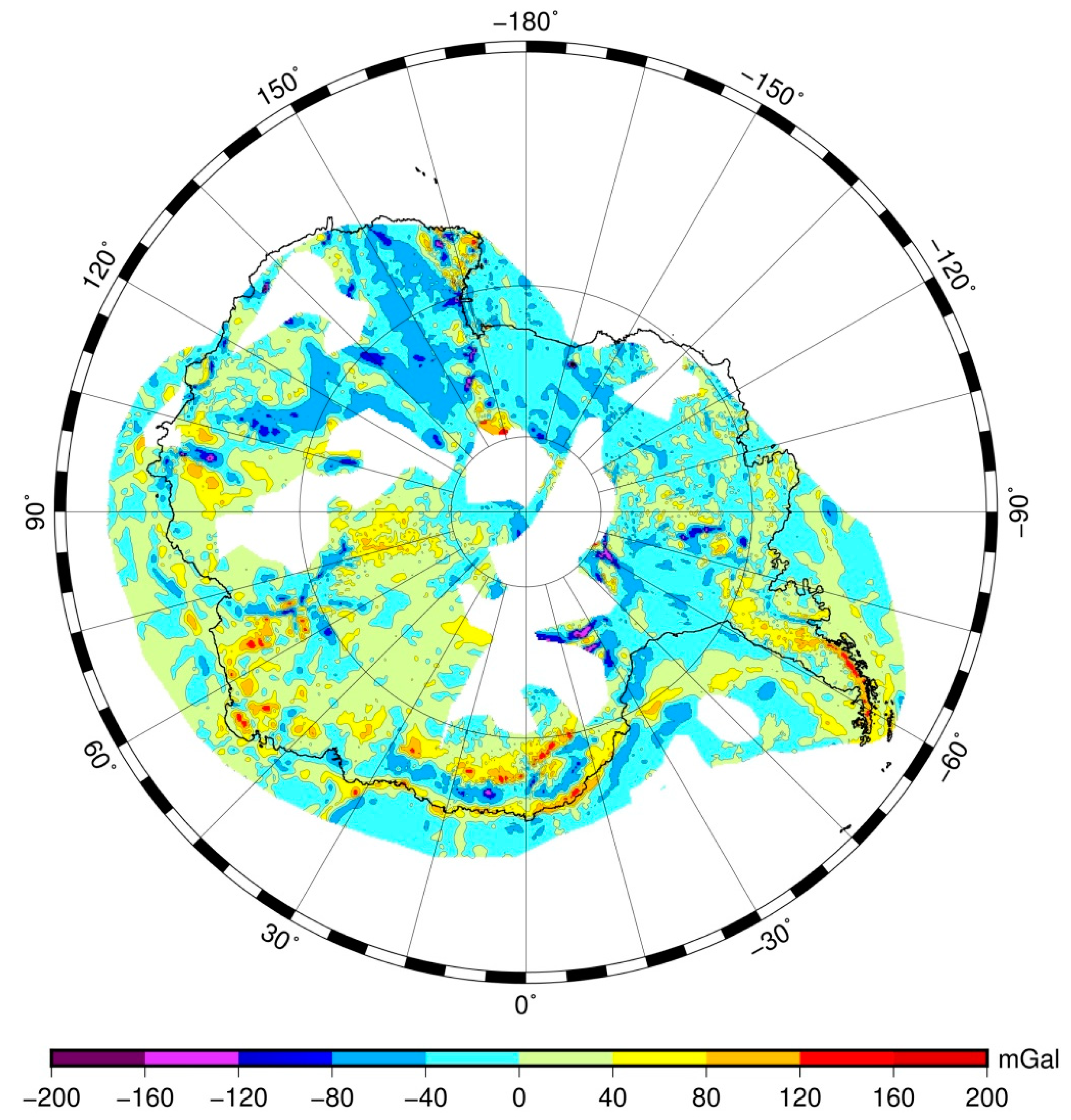
4.1. Free Air Gravity (FAG) Anomaly Interpretation

NVL is characterized by the irregular spatial distribution of the FAG anomaly which includes the highest and lowest values. FAG anomalies in the Ross Sea are close to zero and assume a N–S trend as in the Terror Rift, Victoria Land Basin and Central Trough (Figure 11). The TAM (Trans Antarctic Mountains) is associated with positive values and is interrupted by a very strong negative minimum value (about −200 mGal) at the 75°S parallel. A second interruption, again with a similar strong negative minimum value, is present at the 79°S, south of McMurdo Sound. Mt. Erebus and Mt. Melbourne, the active volcanoes in this region, have associated positive maxima. The Rennick Geodynamic Belt is characterized by an abrupt step from −200 mGal (to the West) to +160 mGal (on the NE side). Its influence on the topography is evident in the FAG anomaly map that suggests its SE continuation to the Lanterman Range. Along the Lillie–Tucker fault another negative minimum zone is present in its NW sector (−150 mGal) whereas in the SE sector a step from −100 mGal (SW) to +200 mGal (NE) is present. The latter is due to the Admiralty Mts.
At the continental scale, FAG anomaly of Antarctica evidences the main peaks. Together with VL and the TAM, Gambursev Mts, Antarctica Peninsula, Dronning Maud Land, mountains of Enderby, Mac Robertson, and Queen Mary lands can be tracked. In FAG anomaly of Antarctica (Figure 12) the continuation of TAM to the South is well visible and is interrupted by a minimum negative zone around about the 81°S parallel. Four regional main depressions, the Ross and Weddel Sea, the Wilkes and Aurora Basin, are evident in the map as zones with negative values (from about −80 to −40 mGal). A series of narrow sharp negative minima characterize both East and West Antarctica. In West Antarctica is present a narrow depression immediately to the East of the Ellsworth Mts, while the nearby Bentley Trench does not seem to show a significant correlation with the FAG anomaly. In East Antarctica, several sharp negative minima are present to the West of Pensacola Mts, in the Coats Land, in the Lambert Rift and its inland propagation towards the foothill of the Gamburtsev Mts, in the Vostok Lake, in the northern Queen Mary Land, in the Adventure Trench and W to Mawson Peninsula. A further negative zone girdles the northern part of Dronning Maud Land.

4.2. Bouguer Gravity (BG) Anomaly Interpretation

The BG anomaly represents the gravitational action because of the material existing below the considered surface. A large mountain chain causes the lithosphere deflection as consequence of the phenomenon of Airy’s isostatic compensation. Since the Bouguer correction does not take into account the roots of the mountains, BG anomalies above mountains are negative and above oceans are positive. The mantle rocks, which are more dense than the crustal ones, are at a lower depth in oceanic areas and at greater depths under the continental mountains. This generates, respectively, relative excesses and gravity defects, which in Bouguer’s maps are characteristic of isostatic conditions. BG anomaly map gives a clear idea of subsurface density. Negative values imply lower density beneath the measurement point, while the positive ones indicate higher density. Positive anomalies generally indicate the presence of thin crust (about 20 km), which is evident where the Moho rises. Offshore, FAG anomalies are comparable in size and shape with BG anomalies mainly due to shallow-water and uniform bathymetry. Negative BG anomalies with a large wavelength under the mountains are related to well-defined crustal roots and indicate the presence of lithosphere subduction [55].
The BG anomaly map (Figure 9) evidences the presence of two regions: the Ross Sea is characterized by positive values while negative values are present in the VL. The BG anomaly in the Ross Sea shows rather homogeneous values with relative maxima corresponding to the Victoria Land Basin and Central Trough depressions, similarly to the FAG anomaly map (Figure 11). The narrow Terror Rift does not show a marked signature, and it can refer to the local behavior of the lithosphere that elastically sustains it, thus preventing its isostatic counterbalance.
In VL, the BG anomaly shows an East–West gradient with decreasing negative values towards the Ross Sea, as expected for the rift shoulder of an extensional basin (10 Brink). In correspondence of the Bowers Mts, BG anomalies show an abrupt change of over 100 mGal as highlighted by Ferraccioli [56]. This change may relate to the presence of a step in the Moho depth along the Rennick Geodynamic Belt (Figure 1). On the other hand, the apparent regional lack of such a step at regional scale points to the strike-slip role of this geodynamic belt. The negative values associated with Mt. Erebus are an indication of the presence of its root (local crustal thickening), and are possibly due to the presence of intrusions or alternatively to flexural roots (e.g., Aitken [57]). This evidence contrasts with the absence of anomaly at the other active volcano, Mt. Melbourne. The irregular spatial distribution of the anomaly values, which characterize NVL, may be easily related to local transpression/transtension due to the activity of the strike-slip tectonics produced along the propagation of the Balleny and Tasman fracture zones in Cenozoic times [23]. This strike-slip tectonic regime in NVL is, therefore, responsible for the presence of the scattered anomalies with a radius of the order of few tens of kilometers. This contrasts with the extensional regime along the VL coastline that is clearly depicted by the transition band between positive and negative BG anomalies.
At continental scale, the BG anomaly of Antarctica confirms the dual distribution between East and West Antarctica, with positive values in the latter and negative values in the former. In West Antarctica, negative values correspond to the roots (i.e., larger crustal thickness), at the Antarctic Peninsula, of the Ellsworth Highlands, and of the Mary Byrd Land. In East Antarctica wide negative anomalies are related to the roots of the TAM and of the main subglacial mountains, the Gamburtsev Mts and Dronning Maud Land. Relative negative minima characterize the Resolution Highland.
A wide zone of negative values is present at the highlands between the Gamburtsev Mts and the Dronning Maud Land. The positive anomaly in the Lambert rift confirms the crustal thinning of this region. The large positive values that surround most of the Antarctic coastline represent the effect of the combined thinning of the crust towards the ocean and the border effect of the gridding. The moderate negative values in the Wilkes and Aurora basins may reflect the presence of a buried sedimentary cover as proposed by Scheinert et al. [17] and Jordan et al. [25].

5. Discussion

Gravity anomalies identify two main sectors in NVL. The first is a NW region, which is characterized by small-sized BG anomalies with wavelengths of the order of some tens of kilometers. In this sector, the relative minimum values (differences up to 200 mGal) are sharper than the maximum values (100 mGal), which are associated with high uplift rates (Figure 5). The second sector is a SE region, which shows low BG anomaly values that correspond to general subsiding velocities. The lowest Bouguer values correspond to the roots of the highest elevations (Mt. Murchison) of the region.
Absolute plate velocities between the 140°E and 40°W, including VL and West Antarctica with the Peninsula, are similar in their magnitude, around 10 mm/yr, and direction, roughly around the 135°E meridian. This contrasts with absolute velocities of stations located in the rest of East Antarctica, which are characterized by lower magnitudes and more variable directions. This last point relates to their closer position to the rotation pole.
The comparison between these velocities and the spreading of oceans surrounding Antarctica shows a quite similar trend (Figure 14). The Southern Ocean expansion between 90°E and 140°E is nearly perpendicular to the East Antarctica continental margin and the ridge zone is characterized by few transforms with small offsets. The spreading style of the Southern Ocean changes abruptly between 140°E and 180°E meridians, being characterized by a series of transforms, the Tasman and Balleny fracture zones, that crosscut the whole ocean and propagate on land both in Antarctica [23,24] and Australia [58] with a right lateral motion. As a consequence, the spreading of the Southern Ocean becomes nearly parallel to the NVL coastline.
The pathway of these fracture zones is nearly parallel to the absolute velocity vectors from VL to the Antarctic Peninsula, which represents the only convergent margin of the Antarctic continent.
The pathway of the Balleny and Tasman Fracture Zones is nearly parallel to the absolute velocity vectors from VL to the Antarctic Peninsula (Figure 14), and represents the only convergent margin of the Antarctic continent. This suggests that the activity along these fracture zones is associated with the observed rotation of the Antarctic continent. This relation still leaves the question about the leading mechanism for the clockwise rotation of Antarctica open, i.e., being the effect of differential ocean spreading or due to an active continent rotation accommodated by the ocean spreading [59]. The presence of active right-lateral offset along the onshore prosecution of these fracture zone into NVL [21,23,24] suggests that the former hypothesis better describes the present-day geodynamic environment of the Antarctic continent and the engine reasonably resides in the mantle flow associated with the ocean spreading. The presence of the Cenozoic deformation belt in East Antarctica Craton [22,60] characterized by the presence of a subglacial lake cluster [61,62], could well represent the effect of this ocean-driven rotation.
The activity role of the Tasman and Balleny fracture zones is limited along their zone of influence as in the NVL and the absolute vertical velocities confirm this framework. The general uplift in the Antarctic Peninsula and in the eastern part of West Antarctica is characterized by locations with movements exceeding 10 mm/yr and up to over 50 mm/yr (see in Figure 7 the stations indicated with a black star). These values are larger than ones predicted by the GIA models [63,64] and may easily relate to the active tectonics, including the presence of converging margins. The tilting in NVL is the effect of the activity of the on-land southern propagation of the fracture zones. In the other regions of East Antarctica, closer to the plate rotation pole and characterized by a direction of ocean spreading perpendicular to the continent margins, there are not significant vertical movements.

6. Conclusions

From the analysis of the observed GNSS data collected in a time span of about 20 years, improvement in the velocity uncertainty was obtained together with a new global framework of the Antarctic geodynamic behavior. New detailed gravimetric maps were elaborated merging original terrestrial datasets with airborne and shipborne data. The updated geodetic and gravimetric maps’ interpretation permits us to highlight the geodynamic characteristics of Victoria Land (VL) in the frame of the Antarctic plate motion.
The Victoria Land Network for Deformation control (VLNDEF) processing highlights a movement of VL towards the SE (Ve 9.9 ± 0.26 mm/yr, Vn −11.9 ± 0.27 mm/yr) with a pathway nearly parallel to the transforms, which start from the Tasman and Balleny fracture zones and propagate on land in Antarctica. The velocity difference between East and West Antarctica is due to the close position of the rotation pole to East Antarctica while the similarity between VLNDEF_2018 and ITRF14 poles shows that ITRF14 system is well defined in Antarctica.
BG anomalies confirm the differences between the thickness of the Earth’s crust of East and West Antarctica, while the relative velocities of the Antarctic stations demonstrate that the movements between the two regions are negligible. Some exceptions are due to stations that show active regional tectonics. NVL data confirm the highest uplift rates, while in the sector between 73°S and 74°S significant subsidence due to the right-lateral offset along the on land reactivated NNW–SSE regional faults was detected. The BG anomaly maps show the thinning of the crustal thickness from VL toward the Ross Sea. The NW region, characterized by small BG anomaly values, is associated with high uplift rates while the SE region presents low BG anomaly values and corresponding subsidence phenomenon. Unreported density variations produce the lowest BG values in the highest elevations (Mt. Murchison) of the region whereas gravity anomalies are mostly related to vertical movements and evidence the effect of dip-slip tectonics. The GNSS data reveal present day activity of the Rennick Geodynamic Belt, while gravity data is interpreted to support dominantly strike slip movement in this region over the Cenozoic. Tectonic dislocations are detected in the gravity anomaly map along the Rennick Geodynamic Belt, suggesting its southern continuation south of the Lanterman Range. The revealed scattered gravimetric anomalies confirm the differences between the modeled GIA values and the observed uplift values that can be related to deep-seated regional scale structures.

Supplementary Materials

The following are available online at https://0-www-mdpi-com.brum.beds.ac.uk/2072-4292/10/10/1608/s1, Table S1: Time span of the processed GNSS stations. The GNSS dataset consists of VLNDEF (ftp://ftp.ira.inaf.it/pub/ogia/), POLENET (ftp://data-out.unavco.org/pub/rinex/obs/) and IGS (ftp://igs.ensg.ign.fr/pub/igs/data/) stations. In red the stations located in Antarctica, Table S2: List of the processed GNSS stations (4-character codes) and their time span considered. A star (*) before the file name indicate span less than one year while a percentage (%) shows span less than two years but more than one year. The stations marked with a star (*) or with a percentage (%) were not considered reliable due the short time series which were reflected in large uncertainties, Table S3: Antarctic continuous GNSS sites used in this paper. For each year the number of daily observations is given. The last column indicate the accumulated total amount of daily observations, Table S4: The columns display the approximate geographic coordinates and the velocities of the Antarctic stations, Table S5: The columns display the approximate geographic coordinates of the terrestrial points located in VL, the gravity values observed and the gravity anomalies computed. H = orthometric height (Earth Gravitational Model 2008—EGM2008 [43]); BGA = Bouguer Gravity anomaly; FAGA = Free-Air Gravity anomaly; the deviation of the merged gravimetric surface on the fiducial points.

Author Contributions

F.M., M.N., L.V. and A.Z. conceived and designed the paper; A.C., M.D., P.C., F.M., F.S., P.S., L.V. and A.Z. joined in Antarctic Scientific Expeditions; P.S. analyzed the geophysical data; P.C. and F.S. developed the geodynamic and tectonic interpretation of the data results partly within the PNRA, G-IDEA project; L.M., M.N. and A.Z. analyzed the GNSS data. A.C. is the Principal Investigator of geodetic projects supported by PNRA, Co-Chair with Mirko Scheinert (Technische Universität, Dresden, Germany) of the Geodetic Infrastructure of Antarctica (GIANT) Expert Group within the Scientific Committee on Antarctic Research (SCAR). All authors contributed to the writing of the paper.

Funding

Part of this work was supported by the Italian National Program for Antarctic Research (PNRA).

Acknowledgments

Several researchers contributed to the field activities. The figures were produced with the Generic Mapping Tool (GMT) software [65].

Conflicts of Interest

The authors declare no conflict of interest.

References

  1. Argus, D.F.; Peltier, W.R.; Drummond, R.; Moore, A.W. The Antarctica component of postglacial rebound model ICE-6G_C (VM5a) based upon GPS positioning, exposure age dating of ice thicknesses, and relative sea level histories. Geophys. J. Int. 2014, 198, 537–563. [Google Scholar] [CrossRef]
  2. Amalvict, M.; Willis, P.; Wöppelmann, G.; Ivins, E.R.; Bouin, M.-N.; Testut, L.; Hinderer, J. Isostatic stability of the East Antarctic station Dumont d’Urville from longterm geodetic observations and geophysical models. Polar Res. 2009, 28, 193–202. [Google Scholar] [CrossRef]
  3. King, M.A.; Altamimi, Z.; Boehm, J.; Bos, M.; Dach, R.; Elosegui, P.; Fund, F.; Hernández-Pajares, M.; Lavallée, D.; Mendes Cerveira, P.J.; et al. Improved constraints to models of glacial isostatic adjustment: A review of the contribution of ground-based geodetic observations. Surv. Geophys. 2010, 31, 465–507. [Google Scholar] [CrossRef]
  4. King, M.A.; Whitehouse, P.L.; Van der Wal, W. Incomplete separability of Antarctic plate rotation from glacial isostatic adjustment deformation within geodetic observations. Geophys. J. Int. 2016, 204, 324–330. [Google Scholar] [CrossRef]
  5. Thomas, I.D.; King, M.A.; Bentley, M.J.; Whitehouse, P.L.; Penna, N.T.; Williams, S.D.P.; Riva, R.E.M.; Lavallee, D.A.; Clarke, P.J.; King, E.; et al. Widespread low rates of Antarctic glacial isostatic adjustment revealed by GPS observations. Geophys. Res. Lett. 2011, 38. [Google Scholar] [CrossRef] [Green Version]
  6. Sjöberg, L.; Walyeldeen, H.; Horemuz, M. Estimation of crustal motions at the permanent GPS station SVEA, Antarctica from 2005 to 2009. J. Geod. Sci. 2011, 1, 215–220. [Google Scholar] [CrossRef]
  7. Bevis, M.; Kendrick, E.; Smalley, R., Jr.; Dalziel, I.; Caccamise, D.; Sasgen, I.; Helsen, M.; Taylor, F.W.; Zhou, H.; Brown, A.; et al. Geodetic measurements of vertical crustal velocity in West Antarctica and the implications for ice mass balance. Geochem. Geophys. Geosyst. 2009, 10. [Google Scholar] [CrossRef] [Green Version]
  8. Capra, A.; Mancini, F.; Negusini, M. GPS as a geodetic tool for geodynamic in Northern Victoria Land, Antarctica. Antarct. Sci. 2007, 19, 107–114. [Google Scholar] [CrossRef]
  9. Mancini, F. Geodetic activities: A new GPS network for crustal deformation control in northern Victoria Land. Terra Antart. Rep. 2001, 5, 23–28. [Google Scholar]
  10. Zanutta, A.; Vittuari, L.; Gandolfi, S. Geodetic GPS-based analysis of recent crustal motions in Victoria Land (Antarctica). Glob. Planet. Chang. 2008, 62, 115–131. [Google Scholar] [CrossRef]
  11. Llubes, M.; Florsch, N.; Legresy, B.; Lemoine, J.-M.; Loyer, S.; Crossley, D.; Rémy, F. Crustal thickness in Antarctica from CHAMP gravimetry. Earth Planet. Sci. Lett. 2003, 212, 103–117. [Google Scholar] [CrossRef] [Green Version]
  12. Hirt, C.; Rexer, M.; Scheinert, M.; Pail, R.; Claessens, S.; Holmes, S. A new degree-2190 (10 km resolution) gravity field model for Antarctica developed from GRACE, GOCE and Bedmap2 data. J. Geod. 2016, 90, 105–127. [Google Scholar] [CrossRef]
  13. Brockmann, J.M.; Zehentner, N.; Höck, E.; Pail, R.; Loth, I.; Mayer-Gürr, T.; Schuh, W.-D. EGM_TIM_RL05: An independent geoid with centimeter accuracy purely based on the GOCE mission. Geophys. Res. Lett. 2014, 41, 8089–8099. [Google Scholar] [CrossRef] [Green Version]
  14. Hirt, C.; Rexer, M.; Claessens, S.J. Topographic evaluation of fifthgeneration GOCE gravity field models—Globally and regionally. In: Special issue on validation of GOCE gravity fields. Newton’s Bull. 2015, 5, 163–186. [Google Scholar]
  15. Fretwell, P.; Pritchard, H.D.; Vaughan, D.G.; Bamber, J.L.; Barrand, N.E.; Bell, R.; Bianchi, C.; Bingham, R.G.; Blankenship, D.D.; Casassa, G.; et al. Bedmap2: Improved ice bed, surface and thickness data sets for Antarctica. Cryosphere 2013, 7, 375–393. [Google Scholar] [CrossRef] [Green Version]
  16. Forsberg, R.; Olesen, A.V.; Yildiz, H.; Tscherning, C.C. Polar gravity fields from GOCE and airborne gravity. In Proceedings of the 4th International GOCE User Workshop European Space Agency, Munich, Germany, 31 March–1 April 2011. ESA SP-696. [Google Scholar]
  17. Scheinert, M.; Ferraccioli, F.; Schwabe, J.; Bell, R.; Studinger, M.; Damaske, D.; Jokat, W.; Aleshkova, N.; Jordan, T.; Leitchenkov, G.; et al. New Antarctic Gravity Anomaly Grid for Enhanced Geodetic and Geophysical Studies in Antarctica. Geophys. Res. Lett. 2016, 43, 600–610. [Google Scholar] [CrossRef] [PubMed]
  18. Scheinert, M. Progress and prospects of the Antarctic Geoid Project (Commission Project 2.4). In Geodesy for Planet Earth; Kenyon, S., Pacino, M.C., Marti, U., Eds.; International Association of Geodesy Symposia; Springer: Berlin, Germany, 2012; Volume 136, pp. 451–456. [Google Scholar]
  19. Martín-Español, A.; Zammit-Mangion, A.; Clarke, P.J.; Flament, T.; Helm, V.; King, M.A.; Luthcke, S.B.; Petrie, E.; Rémy, F.; Nana, S.; et al. Spatial and temporal Antarctic Ice Sheet mass trends, glacio-isostatic adjustment, and surface processes from a joint inversion of satellite altimeter, gravity, and GPS data. J. Geophys. Res. Earth Surf. 2016, 121, 182–200. [Google Scholar] [CrossRef] [PubMed] [Green Version]
  20. Zanutta, A.; Negusini, M.; Vittuari, L.; Cianfarra, P.; Salvini, F.; Mancini, F.; Sterzai, P.; Dubbini, M.; Galeandro, A.; Capra, A. Monitoring geodynamic activity in the Victoria Land, East Antarctica: Evidence from GNSS measurements. J. Geodyn. 2017. [Google Scholar] [CrossRef]
  21. Dubbini, M.; Cianfarra, P.; Casula, G.; Capra, A.; Salvini, F. Active tectonics in northern Victoria Land (Antarctica) inferred from the integration of GPS data and geologic setting. J. Geophys. Res. Solid Earth 2010, 115. [Google Scholar] [CrossRef] [Green Version]
  22. Cianfarra, P.; Maggi, M. Cenozoic extension along the reactivated Aurora Fault System in the East Antarctic Craton. Tectonophysics 2017, 703, 135–153. [Google Scholar] [CrossRef]
  23. Salvini, F.; Brancolini, G.; Busetti, M.; Storti, F.; Mazzarini, F.; Coren, F. Cenozoic geodynamics of the Ross Sea region, Antarctica: Crustal extension, intraplate strikeslip faulting, and tectonic inheritance. J. Geophys. Res. 1997, 102, 24669–24696. [Google Scholar] [CrossRef]
  24. Storti, F.; Salvini, F.; Rossetti, F.; Phipps Morgan, J. Intraplate termination of transform faulting within the Antarctic continent. Earth Planet. Sci. Lett. 2007, 260, 115–126. [Google Scholar] [CrossRef]
  25. Jordan, T.A.; Ferraccioli, F.; Armadillo, E.; Bozzo, E. Crustal architecture of the Wilkes Subglacial Basin in East Antarctica, as revealed from airborne gravity data. Tectonophysics 2013, 585, 196–206. [Google Scholar] [CrossRef]
  26. Dach, R.; Lutz, S.; Walser, P.; Fridez, P. Bernese GNSS Software Version 5.2; User Manual; Astronomical Institute, University of Bern, Bern Open Publishing: Bern, Switzerland, 2015; ISBN 978-3-906813-05-9. [Google Scholar]
  27. Cerruti, G.; Alasia, F.; Geraiak, A.; Bozzo, E.; Caneva, G.; Lanza, R.; Marson, I. The Absolute Gravity Station and the Mt. Melbourne Gravity Network in Terra Nova Bay, North Victoria Land, East Antarctica. In Recent Progress in Antarctic Earth Science; Yoshida, Y., Ed.; TERRAPUB: Tokyo, Japan, 1992; pp. 589–593. [Google Scholar]
  28. Altamimi, Z.; Rebischung, P.; Métivier, L.; Collilieux, X. ITRF2014: A new release of the International Terrestrial Reference Frame modeling nonlinear station motions. J. Geophys. Res. Solid Earth 2016, 121, 6109–6131. [Google Scholar] [CrossRef] [Green Version]
  29. Gantar, C.; Zanolla, C. Gravity and Magnetic Exploration in the Ross Sea (Antarctica). Boll. Geofis. Teor. Appl. 1993, 35, 219–230. [Google Scholar]
  30. Makinen, J.; Amalvict, M.; Shibuya, K.; Fukuda, Y. Absolute gravimetry in Antarctica: Status and prospects. J. Geodyn. 2007, 43, 339–357. [Google Scholar] [CrossRef]
  31. Tenzer, R.; Chen, W.; Baranov, A.; Bagherbandi, M. Gravity Maps of Antarctic Lithospheric Structure from Remote-Sensing and Seismic Data. Pure Appl. Geophys. 2018, 175, 2181–2203. [Google Scholar] [CrossRef]
  32. Boehm, J.; Werl, B.; Schuh, H. Troposphere mapping functions for GPS and very long baseline interferometry from European Centre for medium-range weather forecasts operational analysis data. J. Geophys. Res. Solid Earth 2006, 111. [Google Scholar] [CrossRef]
  33. Lagler, K.; Schindelegger, M.; Böhm, J.; Krásná, H.; Nilsson, T. GPT2: Empirical slant delay model for radio space geodetic techniques. Geophys. Res. Lett. 2013, 40, 1069–1073. [Google Scholar] [CrossRef] [PubMed] [Green Version]
  34. Negusini, M.; Petkov, B.H.; Sarti, P.; Tomasi, C. Ground-based water vapor retrieval in Antarctica: An assessment. IEEE Trans. Geosci. Remote Sens. 2016, 54. [Google Scholar] [CrossRef]
  35. Steigenberger, P.; Rothacher, M.; Dietrich, R.; Fritsche, M.; Rülke, A.; Vey, S. Reprocessing of a global GPS network. J. Geophys. Res. 2006, 111. [Google Scholar] [CrossRef] [Green Version]
  36. Steigenberger, P.; Rothacher, M.; Fritsche, M.; Ruelke, A.; Dietrich, R. Quality of reprocessed GPS satellite orbits. J. Geod. 2009, 83, 241–248. [Google Scholar] [CrossRef] [Green Version]
  37. Rothacher, M.; Angermann, D.; Artz, T.; Bosch, W.; Drewes, H.; Gerstl, M.; Kelm, R.; König, D.; König, R.; Meisel, B.; et al. GGOS-D: Homogeneous reprocessing and rigorous combination of space geodetic observations. J. Geod. 2011, 85, 679–705. [Google Scholar] [CrossRef]
  38. Tesmer, V.; Steigenberger, P.; Rothacher, M.; Boehm, J.; Meisel, B. Annual deformation signals from homogeneously reprocessed VLBI and GPS height time series. J. Geod. 2009, 83, 973–988. [Google Scholar] [CrossRef]
  39. Carrere, L.; Lyard, F.; Cancet, M.; Guillot, A.; Picot, N. FES 2014, a new tidal model—Validation results and perspectives for improvements. In Proceedings of the ESA Living Planet Conference, Prague, Czech Republic, 9–13 May 2016. [Google Scholar]
  40. Egbert, G.D.; Erofeeva, S.Y. Efficient inverse modeling of barotropic ocean tides. J. Atmos. Ocean. Technol. 2002, 19, 183–204. [Google Scholar] [CrossRef]
  41. Bos, M.S.; Fernandes, R.M.S.; Williams, S.D.P.; Bastos, L. Fast Error Analysis of Continuous GNSS Observations with Missing Data. J. Geod. 2013, 87, 351–360. [Google Scholar] [CrossRef]
  42. Sasgen, I.; Martín-Español, A.; Horvath, A.; Klemann, V.; Petrie, E.J.; Wouters, B.; Horwath, M.; Pail, R.; Bamber, J.L.; Clarke, P.J.; et al. Altimetry, gravimetry, GPS and viscoelastic modeling data for the joint inversion for glacial isostatic adjustment in Antarctica (ESA STSE Project REGINA). Earth Syst. Sci. Data 2018, 10, 493–523. [Google Scholar] [CrossRef] [Green Version]
  43. Riva, R.E.M.; Gunter, B.C.; Urban, T.J.; Vermeersen, L.L.A.; Lindenbergh, R.C.; Helsen, M.M.; Bamber, J.L.; van de Wal, R.S.W.; van den Broeke, M.R.; Schutz, B.E. Glacial isostatic adjustment over Antarctica from combined ICESat and GRACE satellite data. Earth Planet. Sci. Lett. 2009, 288, 516–523. [Google Scholar] [CrossRef]
  44. Riva, R.E.M.; Frederikse, T.; King, M.A.; Marzeion, B.; van den Broeke, M. Brief communication: The global signature of post-1900 land ice wastage on vertical land motion. Cryosphere 2016. [Google Scholar] [CrossRef]
  45. Pavlis, N.K.; Holmes, S.A.; Kenyon, S.C.; Factor, J.K. The development and evaluation of the Earth Gravitational Model 2008 (EGM2008). J. Geophys. Res. 2012, 117, B04406. [Google Scholar] [CrossRef]
  46. Munk, W.H.; Cartwright, D.E. Tidal spectroscopy and prediction. Philos. Trans. R. Soc. Lond. A 1966, 259, 533–581. [Google Scholar] [CrossRef]
  47. Agnew, D.C. Earth tides. In Treatise on Geophysics and Geodesy; Herring, T., Ed.; Elsevier: New York, NY, USA, 2007; Volume 3, pp. 163–195. ISBN 978-0-444-53460-6. [Google Scholar]
  48. Lowrie, W. Fundamentals of Geophysics; Cambridge University Press: Cambridge, UK, 2004; ISBN 0-521-46164-2. [Google Scholar]
  49. Cassinis, G.; Dore, P.; Ballarin, S. Fundamental Tables for Reducing Gravity Observed Values; Tipografia Legatoria Mario Ponzio: Pavia, Italy, 1937; pp. 11–27. [Google Scholar]
  50. Liu, H.; Jezek, K.C.; Li, B.; Zhao, Z. Radarsat Antarctic Mapping Project Digital Elevation Model, Version 2; NASA National Snow and Ice Data Center, Distributed Active Archive Center: Boulder, CO, USA, 2015. [Google Scholar]
  51. Forsberg, R.; Tscherning, C.C. Overview Manual for the GRAVSOFT Geodetic Gravity Field Modelling Programs, 2nd ed.; Technical Report; DTU-Space: Kongens Lyngby, Denmark, 2008. [Google Scholar]
  52. Baranov, A.; Tenzer, R.; Bagherbandi, M. Combined gravimetric-seismic crustal model for Antarctica. Surv. Geophys. 2018, 39, 23–56. [Google Scholar] [CrossRef]
  53. Goudarzi, M.; Cocard, M.; Santerre, R. EPC: Matlab software to estimate Euler pole parameters. GPS Solut. 2014, 18, 153–162. [Google Scholar] [CrossRef]
  54. Altamimi, Z.; Métivier, L.; Rebischung, P.; Rouby, H.; Collilieux, X. ITRF2014 plate motion model. Geophys. J. Int. 2017, 209, 1906–1912. [Google Scholar] [CrossRef]
  55. Fowler, C.M.R. The Solid Earth: An Introduction to Global Geophysics, 2nd ed.; Cambridge University Press: Cambridge, UK, 2005; pp. 205–206. ISBN 0-521-89307-0. [Google Scholar]
  56. Ferraccioli, F.; Bozzo, E.; Capponi, G. Aeromagnetic and gravity anomaly constraints for an early Paleozoic subduction system of Victoria Land, Antarctica. Geophys. Res. Lett. 2002, 29, 44.1–44.4. [Google Scholar] [CrossRef]
  57. Aitken, A.R.A.; Wilson, G.S.; Jordan, T.; Tinto, K.; Blakemore, H. Flexural controls on late Neogene basin evolution in southern McMurdo Sound, Antarctica. Glob. Planet. Chang. 2012, 80–81, 99–112. [Google Scholar] [CrossRef]
  58. Lesti, C.; Giordano, G.; Salvini, F.; Cas, R. Volcano tectonic setting of the intraplate, Pliocene-Holocene, Newer Volcanic Province (southeast Australia): Role of crustal fracture zones. J. Geophys. Res. 2008, 113, B07407. [Google Scholar] [CrossRef]
  59. Müller, R.D.; Sdrolias, M.; Gaina, C.; Roest, W.R. Age, spreading rates, and spreading asymmetry of the world’s ocean crust. Geochem. Geophys. Geosyst. 2008, 9, Q04006. [Google Scholar] [CrossRef]
  60. Cianfarra, P.; Salvini, F. Origin of the Adventure Subglacial Trench linked to Cenozoic extension in the East Antarctic Craton. Tectonophysics 2016, 670, 30–37. [Google Scholar] [CrossRef]
  61. Tabacco, I.E.; Cianfarra, P.; Forieri, A.; Salvini, F.; Zirizotti, A. Physiography and tectonic setting of the subglacial lake district between Vostok and Belgica subglacial highlands (Antarctica). Geophys. J. Int. 2006, 165, 1029–1040. [Google Scholar] [CrossRef] [Green Version]
  62. Cianfarra, P.; Forieri, A.; Salvini, F.; Tabacco, I.E.; Zirizotti, A. Geological setting of the Concordia Trench-Lake system in East Antarctica. Geophys. J. Int. 2009, 177, 1305–1314. [Google Scholar] [CrossRef] [Green Version]
  63. Whitehouse, P.L.; Bentley, M.J.; Le Brocq, A.M. A deglacial model for Antarctica: Geological constraints and glaciological modelling as a basis for a new model of Antarctic glacial isostatic adjustment. Quat. Sci. Rev. 2012, 32, 1–24. [Google Scholar] [CrossRef]
  64. Whitehouse, P.L.; Bentley, M.J.; Milne, G.A.; King, M.A.; Thomas, I.D. A new glacial isostatic adjustment model for Antarctica: Calibrated and tested using observations of relative sea-level change and present-day uplift rates. Geophys. J. Int. 2012, 190, 1464–1482. [Google Scholar] [CrossRef]
  65. Wessel, P.; Smith, W.H.F. Free software helps map and display data. EOS Trans. Am. Geophys. Union 1991, 72, 441–446. [Google Scholar] [CrossRef]
Figure 1. (a) Main physiographic features of the Antarctica continent from Bedmap-2 dataset [15] and (b) simplified tectonic setting of Victoria Land (VL), modified from [20].
Remotesensing 10 01608 g001
Figure 2. Overview over the location of Global Navigation Satellite System (GNSS) stations and gravity sites used in the present work. The top-left inset shows locations of terrestrial gravimetric measurements. The cyan color defines the area where British Antarctic Survey (BAS) airborne data are available [25]; the yellow color identifies an area covered with shipborne gravimetric data [20]; white color defines the areas not covered by airborne and shipborne data. The top-right inset depicts the Victoria Land Network for Deformation control (VLNDEF) network, surveyed in the frame of the Italian National Program for Antarctic Research (PNRA) over 20 years.
Remotesensing 10 01608 g002
Figure 3. Locations of the 208 GNSS stations distributed worldwide and providing data under the supervision of different projects and institutions: VLNDEF (ftp://ftp.ira.inaf.it/pub/ogia/), Polar Earth Observing Network (POLENET) (ftp://data-out.unavco.org/pub/rinex/obs/) and International GNSS Service (IGS) (ftp://igs.ensg.ign.fr/pub/igs/data/); Supplementary Materials available, Tables S1–S3); yellow triangles identify IGS stations adopted to define the geodetic datum within the processing of the GNSS data using Bernese GNSS software [26].
Remotesensing 10 01608 g003
Figure 4. Absolute horizontal displacement map (mm/yr) in Victoria Land (±σ).
Remotesensing 10 01608 g004
Figure 5. Absolute horizontal displacement map (mm/yr) at continental scale (±σ).
Remotesensing 10 01608 g005
Figure 6. Vertical rates (mm/yr) detected in Victoria Land. Red dots denote uplifting sites, blue dots denote subsiding sites. Gray dots show not significant movements following the ±σ criteria. LTF: Lillie–Tucker Fault; RAF: Rennick–Aviator Fault.
Remotesensing 10 01608 g006
Figure 7. Vertical rates (mm/yr) detected at continental scale. Red dots denote uplifting sites, blue dots denote subsiding sites, black stars represent the out of range displayed values (BENN 10.8 ± 1.46 mm/yr, BERP 28.9 ± 2.3 mm/yr, DUPT 12.0 ± 0.74 mm/yr, FONP 13.9 ± 0.77 mm/yr, SPGT 10.2 ± 1.29 mm/yr, TOMO 55.4 ± 3.58 mm/yr; Supplementary Materials, Table S4); gray dots show not significant movements (±σ).
Remotesensing 10 01608 g007
Figure 8. Residual horizontal displacement map (mm/yr) in Victoria Land (±σ).
Remotesensing 10 01608 g008
Figure 9. Residual horizontal displacement map (mm/yr) at continental scale (±σ).
Remotesensing 10 01608 g009
Figure 10. Gridded data of Bouguer Gravity (BG) anomalies (mGal) in Victoria Land (contour interval at 50 mGal).
Remotesensing 10 01608 g010
Figure 11. Gridded data of BG anomalies (mGal) at continental scale (contour interval at 50 mGal).
Remotesensing 10 01608 g011
Figure 12. Gridded data of Free-Air Gravity (FAG) anomalies (mGal) in Victoria Land (contour interval at 40 mGal).
Remotesensing 10 01608 g012
Figure 13. Gridded data of FAG anomalies (mGal) at continental scale (contour interval at 40 mGal).
Remotesensing 10 01608 g013
Figure 14. Absolute velocities of the Antarctica continent within the frame of the Southern Hemisphere plate tectonics focused in the last 70 Ma (orthographic projection, ocean floor age data from [59]). The clockwise rotation of Antarctica is associated with the ocean expansion nearly always at high angle with the continent margins. This contrast with the geodynamic in the Victoria Land, where, related to the eccentric position of the rotation pole with respect to Antarctica, the Tasman and Balleny fracture zones have entered within the continent with an extra right-lateral displacement since the Upper Cenozoic [21,23,24].
Remotesensing 10 01608 g014
Table 1. Occupation (days) of VLNDEF stations from 1998 to 2017.
ID\yr9899000102030405060708091011121314151617
TNB13918133136133435633032936227544182083641673229084365341
VL01-2--1888631168-3510010447106136109365366365
VL02-62-119-48-----14-16---
VL03-62--16-319-10---12-33---
VL04----316-32---16---17---
VL05-4--2143342637-49101891179167118736576
VL06--1--1536-17-----2152125--
VL07-45-615-710-7-15-15-33---
VL08--6--9--13-9---6-423--
VL09-62--19--13-5---9-13---
VL10-44--25341133-4-----12---
VL11--4--7--17----46-13---
VL12-62-552552636-10---7-15365366365
VL13-27--10--13-7-7-13-329--
VL14-102--45342626-5-4-15-10---
VL15--6--18--7--217414--26--
VL16--8--1511-13-7151--20---
VL17--6--2746-13--1-5--330--
VL18--4--117-13--11281335314814512913060
VL19--4--952-11--126---28--
VL21-41-22-10--3-3-8-203--
VL22-23-52-9--5---6-213--
VL23-----402642-----13-15---
VL29-13-32-11------9-213--
VL30--2-32-5------9-11365366365
VL32-2--132-139-----16-18---
VLHG--2----2221--------26--
Table 2. Parameters and models used in the GNSS data processing.
Solid Earth tideIERS Conventions
Permanent tideConventional tide free system: IERS Conventions
Ocean TidesFES2004 (a)
Pole TidesLinear trend for mean pole offsets: IERS Conventions
Ocean LoadingFES2014b + TPXO8-Atlas including the CoM correction for the motion of the Earth due to the ocean tides (b)
Atmospheric LoadingNot applied
A priori informationIGS weekly ERP files (X-pole. Y-Pole, UT1-UTC) used with IGS Precise orbits IG2 (c)/IGS (d)
Subdaily EOP ModelIERS2010
NutationIAU2000R06
Hydrostatic delayComputed from 6-hourly ECMWF grids (e)
Mapping functionsVMF1
Wet delayZero a priori model, 1 –h parameter estimated
GradientsZero a priori values, 24-h parameter estimated
Phase center modeligs14.atx (e)
Radome Calibrationsigs14.atx (e)
Antenna heightigs.snx (e)
Horizontal offsetsApplied
A priori radiation pressureC061001
A priori ionosphere modelCODE GIMs (f)
Table 3. Coordinates and velocities of VLNDEF sites.
Absolute Velocities (mm/yr) Relative Velocities (mm/yr)
IDLon. (°)Lat. (°)H (m)Ve±σeVn±σnVu±σuVeVnVen±σen
TNB1164.10294−74.6988172.2100.15−12.10.160.50.39−0.01−0.250.250.22
VL01169.72507−72.45014596.912.10.18−11.70.22−0.40.450.33−0.340.470.28
VL02167.37814−72.564882047.211.70.24−10.70.2−0.40.380.440.820.930.31
VL03162.92641−72.950512469.6110.23−120.26−0.40.50.73−0.040.730.35
VL04169.74865−73.518211834.611.80.18−11.90.18−1.30.460.31−0.590.670.25
VL05169.61219−73.06307478.511.80.16−11.40.21−0.80.330.24−0.070.250.26
VL06164.69065−74.35000267110.40.18−120.170.80.550.18−0.170.250.25
VL07165.37930−73.759902039.29.90.28−11.80.13−1.40.61−0.65−0.070.650.31
VL08163.73953−73.764282655.410.50.15−11.90.370.90.380.27−0.030.270.40
VL09162.16939−73.330782270.410.10.23−11.90.230.40.470.060.090.110.33
VL10162.76859−73.688462619.49.80.24−11.90.26−0.40.56−0.220.130.260.35
VL11162.54167−74.371432362.39.80.25−11.50.14−0.80.25−0.030.50.500.29
VL12163.72700−72.27444193310.90.12−12.80.250.50.420.21−0.90.920.28
VL13162.20497−74.847801460.39.20.21−11.60.1500.31−0.360.450.580.26
VL14165.90570−73.22825208411.30.21−120.25−0.80.480.53−0.270.590.33
VL15163.71567−74.93426−28.19.40.26−120.130.50.38−0.46−0.080.470.29
VL16162.54549−75.23256311.310.10.23−12.40.160.60.420.54−0.430.690.28
VL17161.53874−75.09513683.58.80.27−11.90.130.70.36−0.540.20.580.30
VL18162.59371−75.89853589.10.15−11.90.210.35−0.180.050.190.25
VL19161.78161−75.80497809.88.80.14−11.80.190.90.45−0.340.230.410.24
VL21163.73293−71.668661899.48.40.52−11.70.2210.15−2.490.232.500.56
VL22162.04043−71.42187274.910.70.19−12.10.252.50.190.12−0.040.130.31
VL23170.30467−71.34582111912.60.21−11.30.330.30.220.41−0.050.410.39
VL29163.89628−71.154081624.411.30.05−11.90.292.80.530.25−0.010.250.29
VL30162.52514−70.598721491.510.60.24−12.60.231.40.46−0.31−0.590.670.33
VL32166.16457−71.73310178412.20.3−12.50.370.70.310.88−0.861.230.48
VLHG162.20172−75.39797165.69.20.17−12.20.110.50.28−0.24−0.160.290.20
Table 4. Euler poles rotational coordinates (“mas yr−1” = milliarcsecond/yr; “° Myr−1” = degree/Millions yr).
ModelNS (a)ωx (mas yr−1)ωy (mas yr−1)ωz (mas yr−1)ω (° Myr−1)
VLNDEF_201895−0.260
±0.005
−0.325
±0.004
0.638
±0.016
0.212
±0.004
ITRF14 (b)7−0.248
±0.004
−0.324
±0.004
0.675
±0.008
0.219
±0.002
(a) Number of sites; (b) from [54].

