Identification of the Noise Model in the Time Series of GNSS Stations Coordinates Using Wavelet Analysis

Abstract

Analysis of the time series of coordinates is extremely important in geodynamic research. Indeed, the correct interpretation of coordinate changes may facilitate an understanding of the diverse geophysical processes taking place in the earth’s crust. At present, when rigorously processing global navigation satellite system (GNSS) observations, the influence of deformations in the surface of the earth’s crust is not considered. This article presents signal modelling for the influence on the analysis of noise occurring in the time series of GNSS station coordinates. The modelling of coordinate time series was undertaken using the classic least-squares estimation (LSE) method and the inverse continuous wavelet transform (CWT). In order to determine the type of noise character, the coefficient spectral index was used. Analyses have demonstrated that the nature of noise in measurement data does not depend on the signal estimation method. The differences between classic modelling (LSE) of the time series with annual and semiannual oscillation and signal reconstruction are very small (Δκ = 0.0 ÷ −0.2).

1. Introduction

Global navigation satellite system (GNSS) coordinate time series have many uses, including estimation of the velocity vectors of measurement stations for geodynamic analysis. Changes in coordinate time series, as well as the geodynamic signal, contain geophysical signals that are not eliminated at the stage of observation. These include Atmospheric Pressure Loading (APL), Hydro (Hydrology), and Non-Tidal Ocean Loading (NTOL) [1,2]. Analysis of these factors’ impacts is extremely important for accurate geodynamic interpretation. In official International Terrestrial Reference Frame (ITRF) solutions, the influence of geophysical factors (APL, Hydro, NTOL) [3] is not taken into account, and only annual and semiannual components are deleted from the data for further geodynamic analyses [4]. In turn, previous research [5] has demonstrated that the annual and semiannual components are not congruent with all analysed International GNSS Service (IGS) stations. For some stations, a dominant annual oscillation can be identified for the “North”, “East”, and “Up” components, while for others, the dominant oscillations differ from the one-year period. In addition, through the use of wavelet analysis, it has been demonstrated that the annual and semiannual components are not constant over time, both in terms of amplitude and period length [5].

Noise analysis represents a means of checking whether geophysical influences of a systematic nature are removed from the coordinate time series. In electronics and information theory, noise refers to these random, unpredictable, and unwanted signals or changes in signals that mask the desired content of information [6]. Hence, knowledge of the nature of noise informs understanding regarding the uncertainty of the parameters of useful signals, such as geodynamic or geophysical signals, in the time series of coordinate changes. Analyses of stations belonging to the IGS network have shown that for all stations, noise had the character of colour noise (spectral index being approximately −0.8 ÷ −1.7; note: white noise = 0.0, flicker noise = −1.0, and random walk = −2.0); more information about the spectral index can be found in [7,8,9,10]. The coefficient of spectral index is a good method to determine the noise character in the time series. Similar analyses have also been conducted for local networks of permanent stations, such as the ASG-EUPOS network in Poland. Analyses have demonstrated that the noise occurring in the time series of coordinates shares the character of colour noise for short-term Global Positioning System (GPS) [11] solutions. The influence of seasonal signals on coordinate changes in time series is also hindered by the analysis of tectonic movements in places of high seismic (tectonic) activity [12]. Noise research in geodetic time series is thus useful for developing an understanding of the nature of changes taking place in coordinates. Awareness of the uncertainty of estimating various parameters from time series is particularly critical [13,14,15,16]. The instantaneous value of noise in the time series can be defined as the difference between instantaneous values of coordinates and the instantaneous value of the model describing the changes of these coordinates. This model contains a periodic signal because seasonal oscillations are ubiquitous in the time series of coordinates, and in some cases, the seasonal signal is interpreted as a geophysical signal. Coordinate changes can also be influenced by local environmental effects such as rain, temperature, or earth crust load [17,18,19]. This article presents analysis of noise occurring in the time series of coordinates of selected IGS stations. The authors depart from the classic method of signal modelling—the least-squares estimation (LSE) method—by using signal reconstruction based on wavelet analysis factors. The article presents input data, methodology, as well as examples of analysis. The conclusions were formulated on the basis of a comparison of the results.

2. Data and Processing Strategy

2.1. Input Data

Data in the form of SINEX files from the Center for Orbit Determination in Europe (CODE) study—2nd Data Reprocessing Campaign—were used for analysis. Detailed information regarding reprocessing is included on the website of the study [20]. It should be noted that during the reprocessing of the data, geophysical models (APL, Hydro, and NTOL) were not included in order to weaken or eliminate the influence of these geophysical factors on coordinate changes in the time series. Detailed analyses regarding the impact of geophysical factors on the deformation of the earth’s crust on the basis of geophysical models are included in the paper [5].

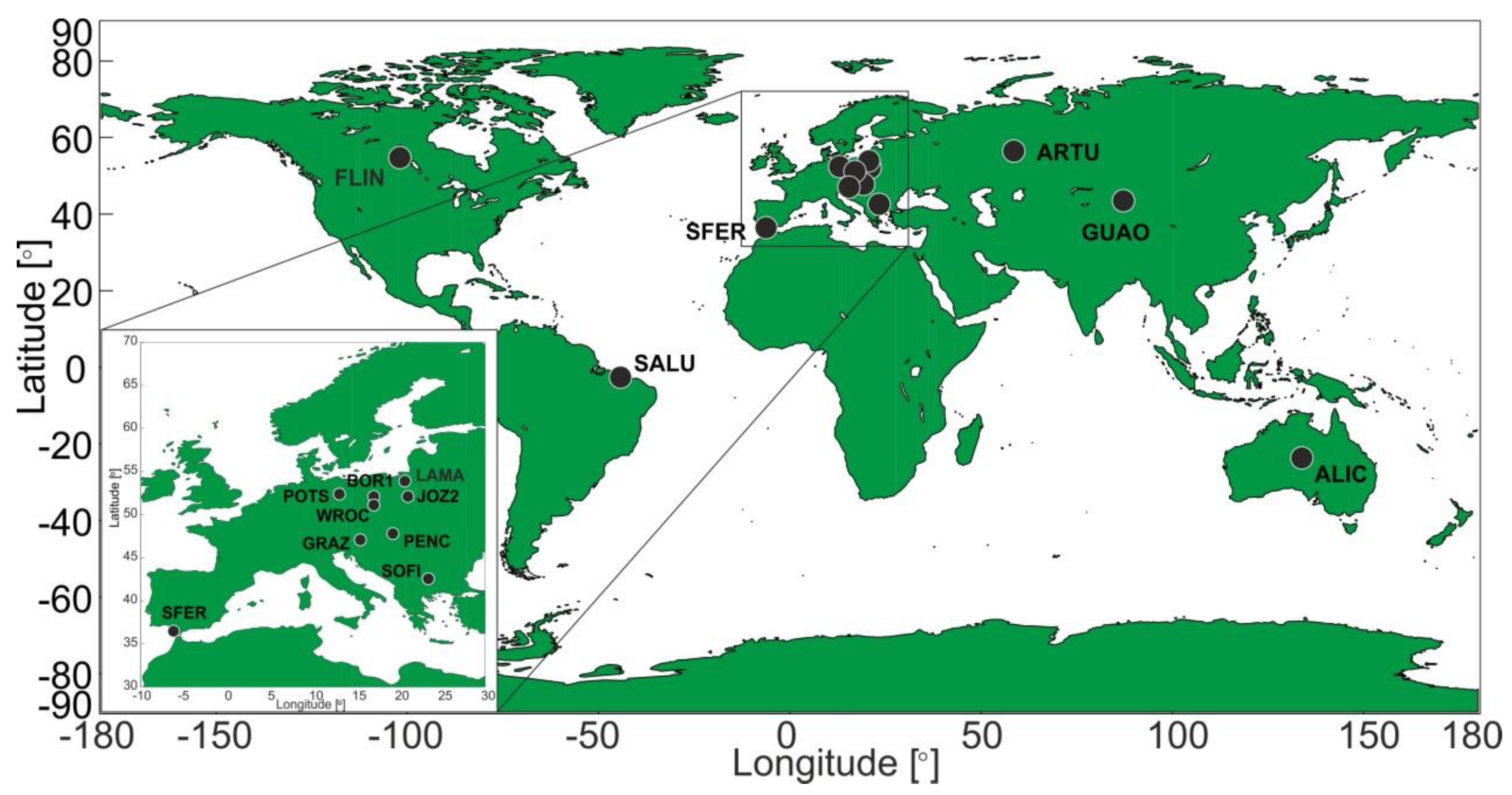
Stations belonging to the IGS network were selected for the research. Stations were chosen at random in order to avoid mutual dependence of the obtained results (Figure 1). The time range of the input data ranged from about 8 to 14 years.

2.2. Methods

The methodology of data elaboration is presented in Section 2.2.1 and Section 2.2.2. It contains the basics of signal reconstruction based on coefficients from wavelet analysis—continuous wavelet transform (CWT)—as well as analysis of the type of noise evident in the measurement data. From the input data, the linear trend was removed using the LSE method.

2.2.1. Signal Reconstruction Function

The most common method of modelling the time series of coordinates comprises classic LSE methods. In this article, a wavelet analysis was used to model the signal, more specifically through the reconstruction of the signal based on the scale coefficients of the previously performed wavelet analysis (CWT). Reconstruction of a signal was treated as a reverse transform. The mother’s “Morlet” wavelet was used for analysis because, for this wavelet alone, the spectrogram is characterised by the chi-squared distribution (Χ²). Formula (1) for signal reconstruction is shown below [21]:

$$x_n=\frac{{\delta }_j\sqrt{{\delta }_t}}{C_{\delta }{\psi }_0\left(0\right)}{\displaystyle \sum }_{j=0}^j\frac{real\left\{W_n\left(s_j\right)\right\}}{\sqrt{s_j}}$$

(1)

where: ${\psi }_0\left(0\right)$—removes the energy scaling;$\sqrt{s_j}$—converts the wavelet transform to an energy density; $C_{\delta }$—reconstruction factor, constant for each wavelet function (

Table 1. Empirically derived factor for wavelet bases [20].

Name of Mother Wavelet	$\mathbf{Reconstruction}\mathbf{Factor}{\mathit{C}}_{\mathit{\delta }}$	$\mathbf{Decorrelation}\mathbf{Factor}\mathbf{for}\mathbf{Tme}\mathbf{Averaging}\mathit{\gamma }$	$\mathbf{Factor}\mathbf{for}\mathbf{Scale}\mathbf{Averaging}{\mathit{\delta }}_{{\mathit{j}}_0}$	$\mathbf{Wavelet}\mathbf{Function}{\mathit{\psi }}_0\left(0\right)$
Morlet (${\omega }_0=6$)	0.766	2.32	0.60	${\pi }^{-1/4}$

); $W_n\left(s_j\right)$—sum of the complex used instead of original time series which were complex; $s$—input signal.

The period of the function was calculated based on the scale and wavelet of the mother using Formula (2):

$$T=\frac{scale}{f_m}$$

(2)

where: $T$—period (days); $f_m$—mother wavelet (Morlet) constant (equal 0.8125).

2.2.2. Analysis of the Character of the Noise

The type of noise that occurs in the time series of coordinates can be determined on the basis of spectral index coefficients [22,23]. Residuals between the input data and the model describing them were analysed. The coefficient “κ” is defined according to Formulas (3) and (4), taking values from −3 to 1 [23]:

$$P_x\left(f\right)=P_0{\left(\frac{f}{f_0}\right)}^{\mathsf{\kappa }}$$

(3)

where: $f$—temporal frequency; $P_0,f_0$—normalizing constants; $\mathsf{\kappa }$—spectral index.

$$\mathsf{\kappa }=\frac{log\left(PSD\right)}{log\left(f\right)}$$

(4)

where: $PSD$—power spectrum density.

The basic types of noise are white noise (κ = 0), flicker noise (κ = −1), and random walk (κ = −2).

3. Results

3.1. Reconstruction of the Signal

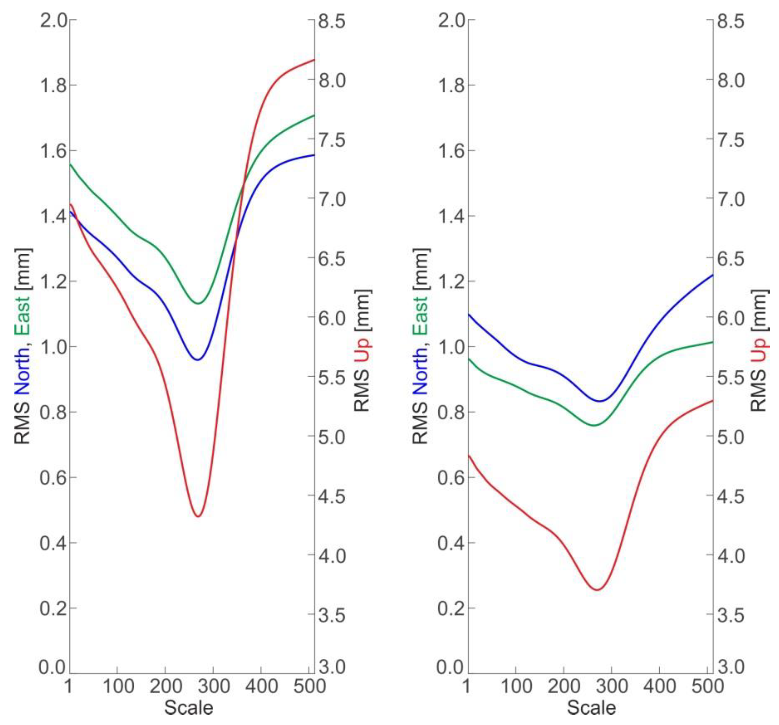
The reconstruction of the signal was undertaken based on Formula (1). For reconstruction, CWT coefficients from the wavelet analysis were used for scales ranging from 1 to 296 (scale 296 corresponds to the annual oscillation of the Morlet wavelet). The choice of CWT analysis coefficients for scales 1:296 was dictated by the fact that for these values, the reconstruction of the signal had the lowest root mean square (RMS). Exemplary RMS dependencies on the accepted scales for signal reconstruction are shown in the following graphs (Figure 2).

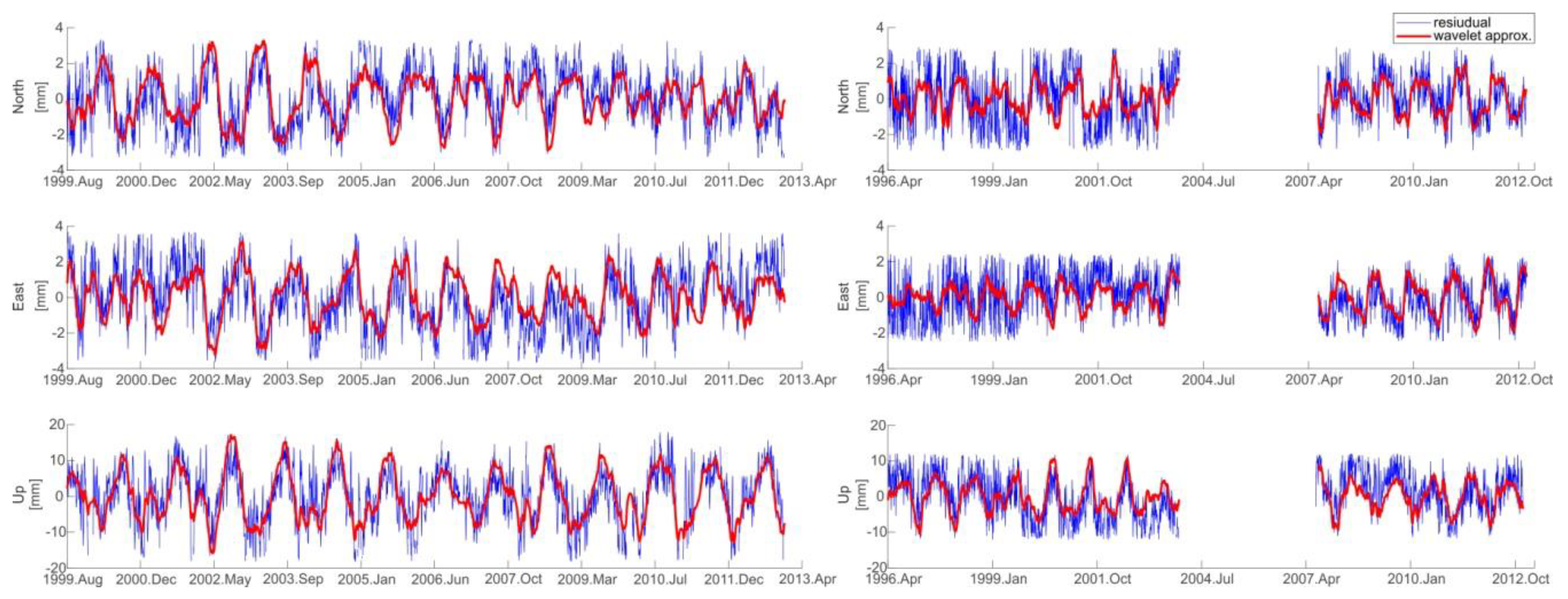
In the graphs (Figure 2), a declining RMS error value can be identified as contingent on the accepted scales for signal reconstruction. Accepting scale values from 1:296 resulted in a marked reduction in RMS. Values of scales above 296 (annual oscillation) cause a sharp increase in RMS error. The time series are too short to clearly state whether time oscillations are longer than one-year periods. An example of a signal reconstruction result for the Arti, Russian Federation (ARTU) and Penc, Hungary (PENC) stations is shown in Figure 3 for scales 1:296.

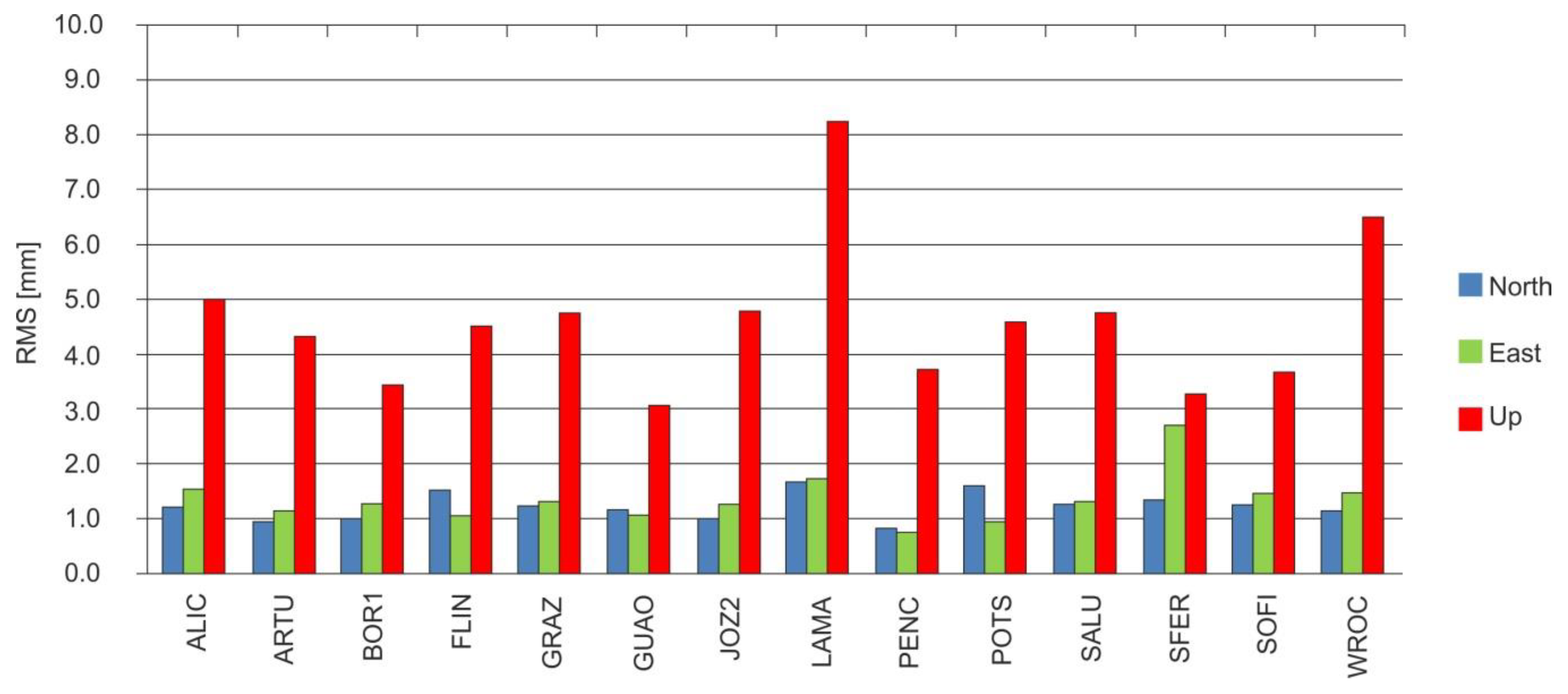
In Figure 3, it can be seen that the signal has been correctly reconstructed, which additionally confirms the RMS error values (for scales 1:296) (Figure 2). For components that are longer than one-year signal reconstructions, the model results are overestimated and the RMS error increases significantly. Confirmation of the signal reconstruction quality for 1:296 scales is provided by the RMS error values (Figure 4). In addition, it can also be noted that the yearly component is the dominant period in the input data for the Up component. For horizontal components, annual oscillation does not occur in the entirety of the time series analysed.

The RMS error values are shown in Figure 4 range from 0.8 to 2.7 mm for the North and East components; for the Up component, these range from 3.1 to 8.2 mm. The values of these errors are smaller than those obtained using the classic least-squares estimation (LSE) method for modelling the time series of coordinates (range from 1.1 to 3.5 mm for the North and East components; for the Up component, these range from 2.5 to 25 mm) [5].

3.2. Fast Fourier Transform (FFT) Analysis

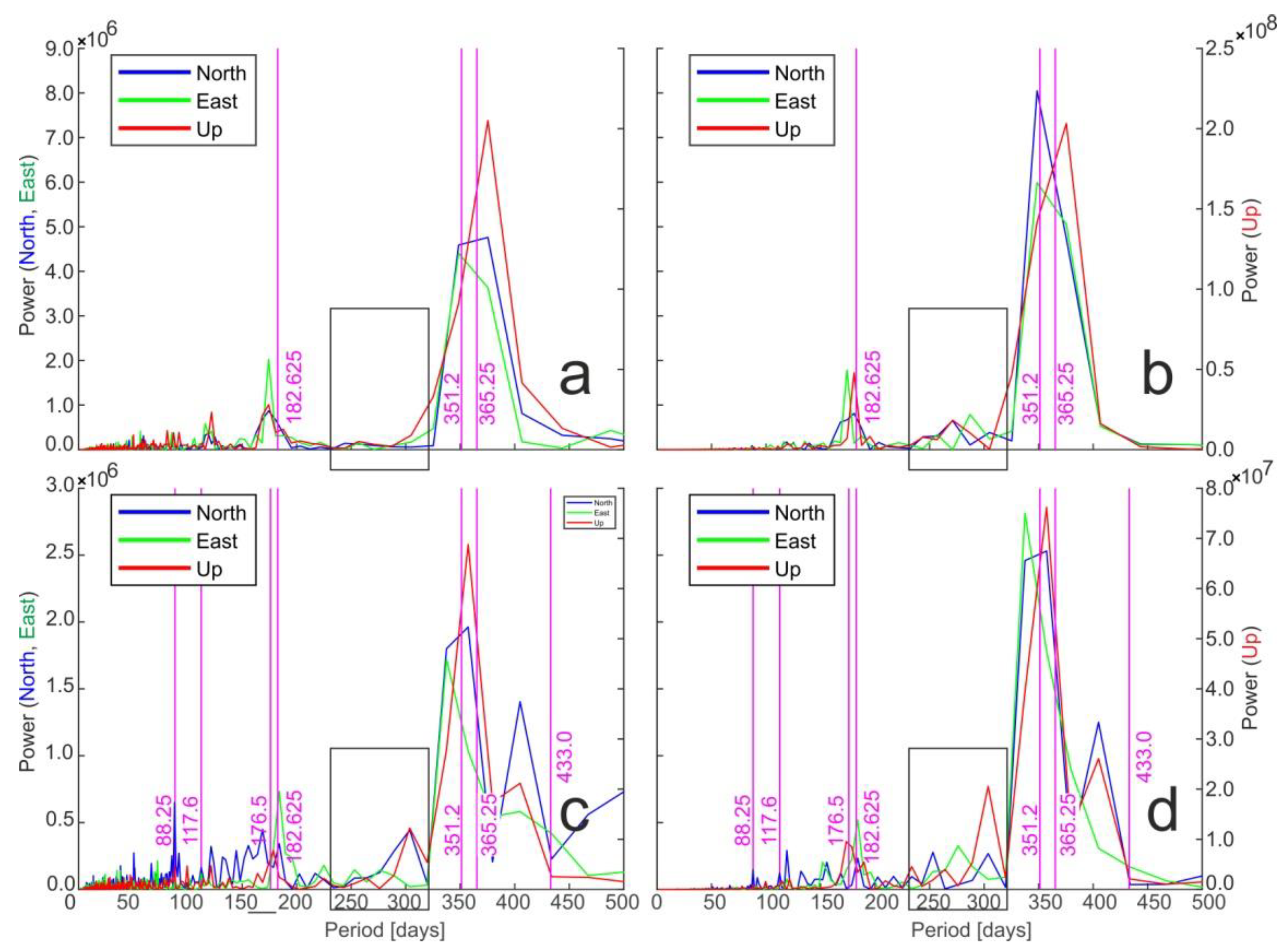
FFT analysis was conducted to verify whether the periodic components of the input and reconstructed signal do not change. It was also used to check whether the annual components are unambiguous for all stations in the North, East, and Up directions. Removing the influence of annual and semiannual components from the data is commonly assumed, but the authors [5] have previously demonstrated that the annual and semiannual components do not have a definite value for the analysed GNSS stations during the entire period under consideration. The classic FFT function has been used here, and the gaps in the data have been supplemented with zero values. Figure 5a,c displays the FFT periodogram for the original signal, while Figure 5b,d shows the FFT periodogram for the reconstructed signal for the ARTU and PENC stations, respectively.

Figure 5 demonstrates that the value of the annual component for the primary and reconstructed signal is not clearly defined for the North, East, and Up directions. There are evident draconic periods (351.2 days for ARTU station—receive GPS data only) as well as components of the tropical year (365.25 days). In addition, for the PENC station (receive GPS + GLONASS data), we can identify an oscillation of approximately 413 days, Chandler oscillation (433 days), 1/4, 1/3, 1/2 of GLONASS draconitic oscillation (they have small power spectrum), and for both stations oscillations of around 280, 300, and 330 days, which were strengthened as a result of signal reconstruction (filtration). These oscillations can be observed at all stations under analysis. The reconstruction, described in detail in Section 2.2., operates similarly to the low-pass filter, which can be seen in Figure 5b,d, where high-frequency attenuation occurs and there is an emphasis on the significant frequencies (increase of their significance).

3.3. Noise Analysis Using the Spectral Index (κ)

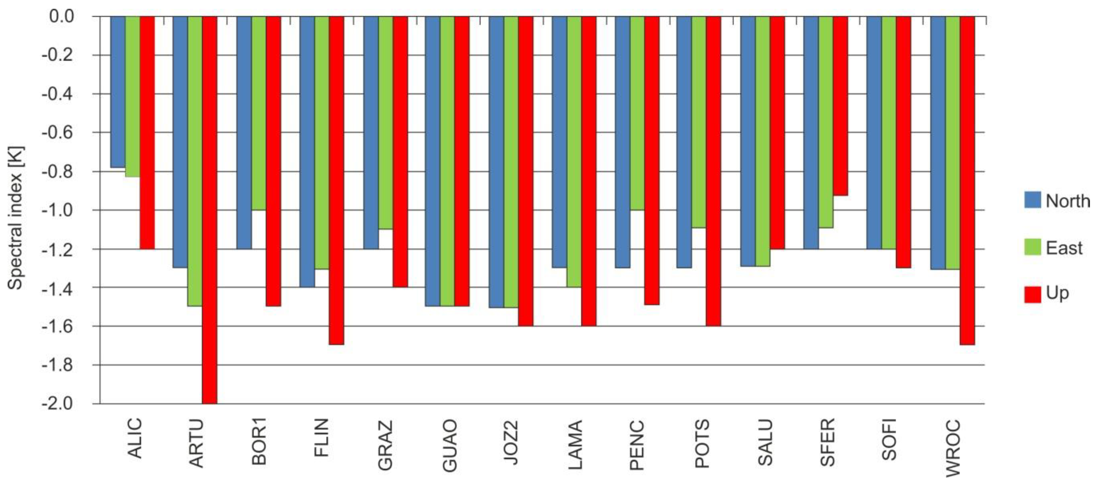
A key element of time-series analysis is the analysis of residuals between the measurement data and the signal model, or so-called noise. The classic LSE method for modelling the time series of coordinates of GNSS stations has been replaced here by the reconstruction of the signal using CWT wavelet analysis, followed by the inverse transform—Formula (1). This constitutes a different approach to signal modelling. The Introduction section highlights that in the time series of coordinates, a colourful noise characterised by a spectral index of around −1 can be identified. In this article, the authors sought to analyse the nature of noise for residues between the data and the reconstructed signal. Figure 6 shows the spectral index coefficients for all analysed IGS stations (Figure 1).

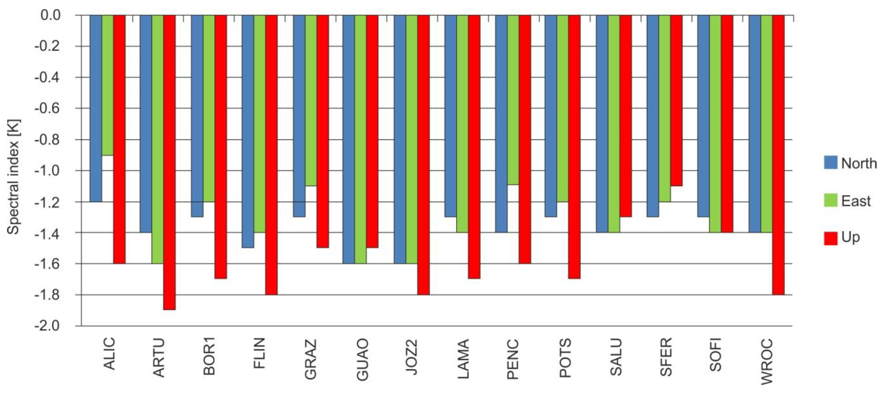
It can be seen that the value of the coefficient κ oscillates within the limits appropriate for the colour noise (flicker noise). In addition, we can see that for some height components Up, the value of the coefficient κ oscillates between −1.5 and −2.0, which may indicate the occurrence of random-walk noise in the data. In order to verify whether the signal reconstruction method does not affect the character of the noise, additional modelling of the input signal was performed using the classic LSE method to estimate the annual and semiannual signal (classic approach), and the noise was analysed (residual between input data and the LSE model). The result of these analyses is shown in Figure 7, where we see that the nature of noise does not change with the use of the LSE method to model the input signal. This may indicate that the type of noise is not dependent on the signal estimation method.

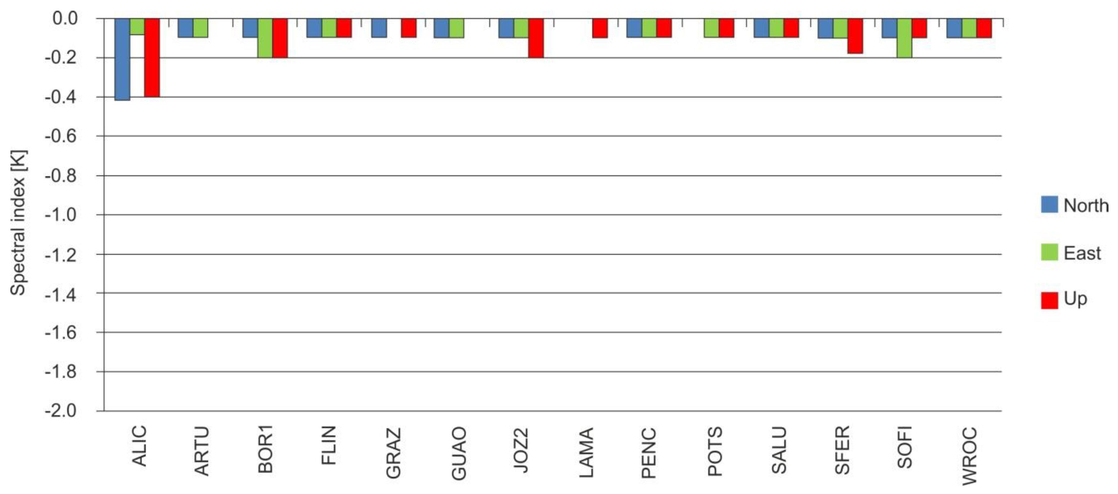
The differences between the two methods of signal modelling (LSE and wavelet signal reconstruction), shown in Figure 8, are small. This confirms that the way in which the signal is modelled does not affect the determination of the character of the noise occurring in the measurement data.

4. Discussion

Analysis of the nature of the noise occurring in the time series of GNSS stations demonstrates that we are dealing with colour noise. This finding confirms the results of other authors, e.g., [24], in which the spectral index coefficient ranged from approximately −0.6 to −1.8 for the stations analysed. Determining the character of noise occurring in the input data is not contingent on the estimation method of the time series model (the LSE method or signal reconstruction based on CWT wavelet coefficients), as confirmed by differences in the spectral index (κ) (Figure 8). This may indicate other, unidentified signals (disturbances) that are not included in the models currently used at the stage of processing GNSS observations. Any possible model will never perfectly reflect real phenomena. During the 2nd GNSS data reprocessing campaign, geophysical signals, such as APL, Hydro, and NTOL, were not included. Indeed, the models that are currently in use are not perfect, and the signals that are unidentified in the coordinate time series are likely to be the result of unidentified disturbances. Determining the cause of the occurrence of colour noise or the phenomenon causing this type of noise constitutes an extremely difficult task. At the analysed stations, annual and semiannual oscillations as well as approximately 182, 280, 300, 330, 351, 365, and 412 days could be identified. Additionally, we can see harmonics of GLONASS draconic year (1/4, 1/3, 1/2) and Chandler osscilation for the PENC station. The yearly oscillation can be linked to the tropical year. However, the oscillation around 351 days can be linked with the GPS draconic year, which is associated with the movement of satellites. For the time series of coordinates shorter than 20 years (we used about 8–14-years long time series), detection of draconic year components for the GLONASS or GPS constellation is difficult [25]. Harmonic oscillations 1/7, 1/5, 1/4, 1/3, 1/2 of the GLONASS draconic year, affect the quality of coordinate solutions, and Earth rotation parameters [26,27]. The above research shows that a signal reconstruction is a good tool for determining the harmonic components occurring in a time series (filtering signal). In addition, it has been proven that the signal modelling method does not affect the type of noise occurring in the signal.

The phenomena (interfering signals) that cause the other oscillations mentioned are difficult to identify. Nevertheless, research in the field continues to take place, providing the potential for increasingly detailed interpretations of geophysical phenomena that can help determine their impact on the results of geodynamic research.

5. Conclusions

The obtained results show that the method of modelling the time series of GNSS coordinates does not significantly influence the determination of the character of the noise occurring in the measurement data. This is confirmed by the difference in the spectral index (Figure 8) between LSE modelling and signal reconstruction using CWT wavelet analysis factors. In addition, the authors advocate estimation of the model of the signal occurring in the coordinate changes of the measurement stations, potentially accounting for all interfering signals; indeed, we currently assume that we can only estimate annual and semiannual signals. This will create the potential for more reliable geodynamic interpretations as well as help identify the reasons behind the colour nature of noise in GNSS coordinates.

References

- Van Dam, T.M.; Blewitt, G.; Heflin, M.B. Atmospheric pressure loading effects on the global positioning system coordinate determinations. J. Geophys. Res. 1994, 99, 23939–23950. [Google Scholar] [CrossRef]
- Tregoning, P.; Watson, C. Atmospheric effects and spurious signals in GPS analyses. J. Geophys. Res. 2009, 114, B09403. [Google Scholar] [CrossRef]
- INTERNATIONAL GNSS SERVICE, CODE Analysis Strategy Summary for IGS repro2. Available online: ftp://ftp.aiub.unibe.ch/REPRO_2013/CODE_REPRO_2013.ACN (accessed on 4 July 2018).
- Dach, R.; Walser, P. Bernese GNSS Software Version 5.2, 3rd ed.; Astronomical Institute, University of Bern: Bern, Switzerland, 2005; ISBN 978-3-906813-05-9. [Google Scholar]
- Kaczmarek, A.; Kontny, B. Estimates of seasonal signals in GNNS time series and environmental loading models with iterative Least-Squares Estimation (iLSE) approach. Acta. Geodyn. Geomater. 2018, 15, 131–141. [Google Scholar] [CrossRef]
- Encyclopædia Britannica. Available online: https://www.britannica.com/ (accessed on 4 July 2018).
- Williams, S.D.P. The effect of coloured noise on the uncertainties of rates estimated from geodetic time series. J. Geod. 2003, 76, 483–494. [Google Scholar] [CrossRef]
- Williams, S.D.P.; Bock, Y.; Fang, P.; Jamason, P.; Nikolaidis, R.M.; Prawirodirdjo, L.; Miller, M.; Johnson, D. Error analysis of continuous GPS position time series. J. Geophys. Res. 2004, 109, B03412. [Google Scholar] [CrossRef]
- Bogusz, J.; Klos, A. On the significance of periodic signals in noise analysis of GPS station coordinates time series. GPS Solut. 2016, 20, 655–664. [Google Scholar] [CrossRef]
- Amiri-Simkooei, A.R.; Tiberius, C.C.J.M.; Teunissen, P.J.G. Assessment of noise in GPS coordinate time series: methodology and results. J. Geophys. Res. 2007, 112, B07413. [Google Scholar] [CrossRef]
- Bogusz, J.; Kontny, B. Estimation of sub-diurnal noise level in GPS time series. Acta Geodyn. Geomater. 2011, 8, 163. [Google Scholar]
- Bos, M.S.; Bastos, L.; Fernandes, R.M.S. The influence of seasonal signals on the estimation of the tectonic motion in short continuous GPS time-series. J Geodyn. 2010, 49, 205–209. [Google Scholar] [CrossRef] [Green Version]
- Zhang, J.; Bock, Y.; Johnson, H.; Fang, P.; Williams, S.; Genrich, J.; Wdowinski, S.; Behr, J. Southern california permanent Gps geodetic array: Error analysis of daily position estimates and sitevelocities. J. Geophys. Res. 1997, 102, 35–55. [Google Scholar] [CrossRef]
- Langbein, J. Noise in GPS displacement measurements from southern California and southern Nevada. J. Geophys. Res. 2008, 113, B05405. [Google Scholar] [CrossRef]
- Santamaría-Gómez, A.; Bouin, M.N.; Collilieux, X.; Wöppelmann, G. Correlated errors in GPS position time series: Implicationsfor velocity estimates. J. Geophys. Res. 2010, 116, B01405. [Google Scholar] [CrossRef]
- Beavan, J. Noise properties of continuous GPS data from concretepillar geodetic monuments in New Zealand and comparison with datafrom U.S. deep drilled braced monuments. J. Geophys. Res. 2005, 110, B08410. [Google Scholar] [CrossRef]
- King, N.E.; Argus, D.; Langbein, J.; Agnew, D.C.; Bawden, G.; Dollar, R.S.; Liu, Z.; Galloway, D.; Reichard, E.; Yong, A.; et al. Space geodetic observation of expansion ofthe San Gabriel Valley, California, aquifer system, during heavy rainfallin winter 2004–2005. J. Geophys. Res. 2007, 112, B03409. [Google Scholar] [CrossRef]
- Prawirodirdjo, L.; Ben-Zion, Y.; Bock, Y. Observation and modeling of thermoelastic strain in Southern California integrated GPS network daily position time series. J. Geophys. Res. 2006, 111, B02408. [Google Scholar] [CrossRef]
- Van Dam, T.; Wahr, J.; Milly, P.C.; Shmakin, A.B.; Blewitt, G.; Lavallée, D.; Larson, K.M. Larson crustal displacements due to continental waterloading. Geophys. Res. Lett. 2001, 28, 651–654. [Google Scholar] [CrossRef]
- International GNSS Service, 2nd Data Reprocessing Campaign. Available online: http://acc.igs.org/reprocess2.html (accessed on 4 July 2018).
- Torrence, C.; Compo, G.P. A practical guide to wavelet analysis. Bull. Am. Meteorol. Soc. 1998, 79, 61–78. [Google Scholar] [CrossRef]
- Mandelbrot, B.B.; Van Ness, J.W. Fractional brownian motions, fractional noises and applications. SIAM Rev. 1968, 10, 422–437. [Google Scholar] [CrossRef]
- Agnew, D. The time-domain behavior of power-law noises. Geophys. Res. Lett. 1992, 19, 333–336. [Google Scholar] [CrossRef]
- Mao, A.; Harrison, C.G.; Dixon, T.H. Noise in GPS coordinate time series. J. Geophys. Res. Solid Earth 1999, 104, 2797–2816. [Google Scholar] [CrossRef] [Green Version]
- Rodriguez-Solano, C.J.; Hugentobler, U.; Steigenberger, P.; Bloßfeld, M.; Fritsche, M. Reducing the draconitic errors in GNSS geodetic products. J. Geod. 2014, 88, 559–574. [Google Scholar] [CrossRef]
- Lutz, S.; Meindl, M.; Steigenberger, P.; Beutler, G.; Sośnica, K.; Schaer, S.; Dach, R.; Arnold, D.; Thaller, D.; Jäggi, A. Impact of the arc length on GNSS analysis results. J. Geod. 2016, 90, 365–378. [Google Scholar] [CrossRef]
- Fritsche, M.; Sośnica, K.; Rodríguez-Solano, C.J.; Steigenberger, P.; Wang, K.; Dietrich, R.; Dach, R.; Hugentobler, U.; Rothacher, M. Homogeneous reprocessing of GPS GLONASS and SLR observations. J. Geod. 2014, 88, 625–642. [Google Scholar] [CrossRef]
Figure 1.
Selected International global navigation satellite system (GNSS) Service (IGS) stations for analysis.
Figure 2.
Examples of root-mean-square (RMS) dependencies on accepted scales for signal reconstruction: Arti, Russian Federation (ARTU) on the left and Penc, Hungary (PENC) on the right.
Figure 3.
Example of signal reconstruction for ARTU (left) and PENC (right) stations.
Figure 4.
RMS error values of the reconstructed signal for the analysed stations.
Figure 5.
Fast Fourier transform (FFT) periodic signal of the source (a: ARTU, c: PENC) and reconstructed signal (b: ARTU, d: PENC). Rectangles show additional peaks before (a,c) and after (b,d) signals reconstruction.
Figure 6.
Spectral index coefficients for the analysed GNSS stations: signal reconstruction as a method of modelling the input signal (κ = 0: white noise, κ = −1: flicker noise, κ = −2: random walk).
Figure 7.
Spectral index coefficients for the analysed GNSS stations: LSE method as a method of modelling the input signal (κ = 0: white noise, κ = −1: flicker noise, κ = −2: random walk).
Figure 8.
Differences in coefficients κ for different methods of estimating the input signal: LSE and signal reconstruction based on wavelet analysis continuous wavelet transform (CWT) coefficients (inverse transform).