Identifying Collapsed Buildings Using Post-Earthquake Satellite Imagery and Convolutional Neural Networks: A Case Study of the 2010 Haiti Earthquake


Abstract
:1. Introduction
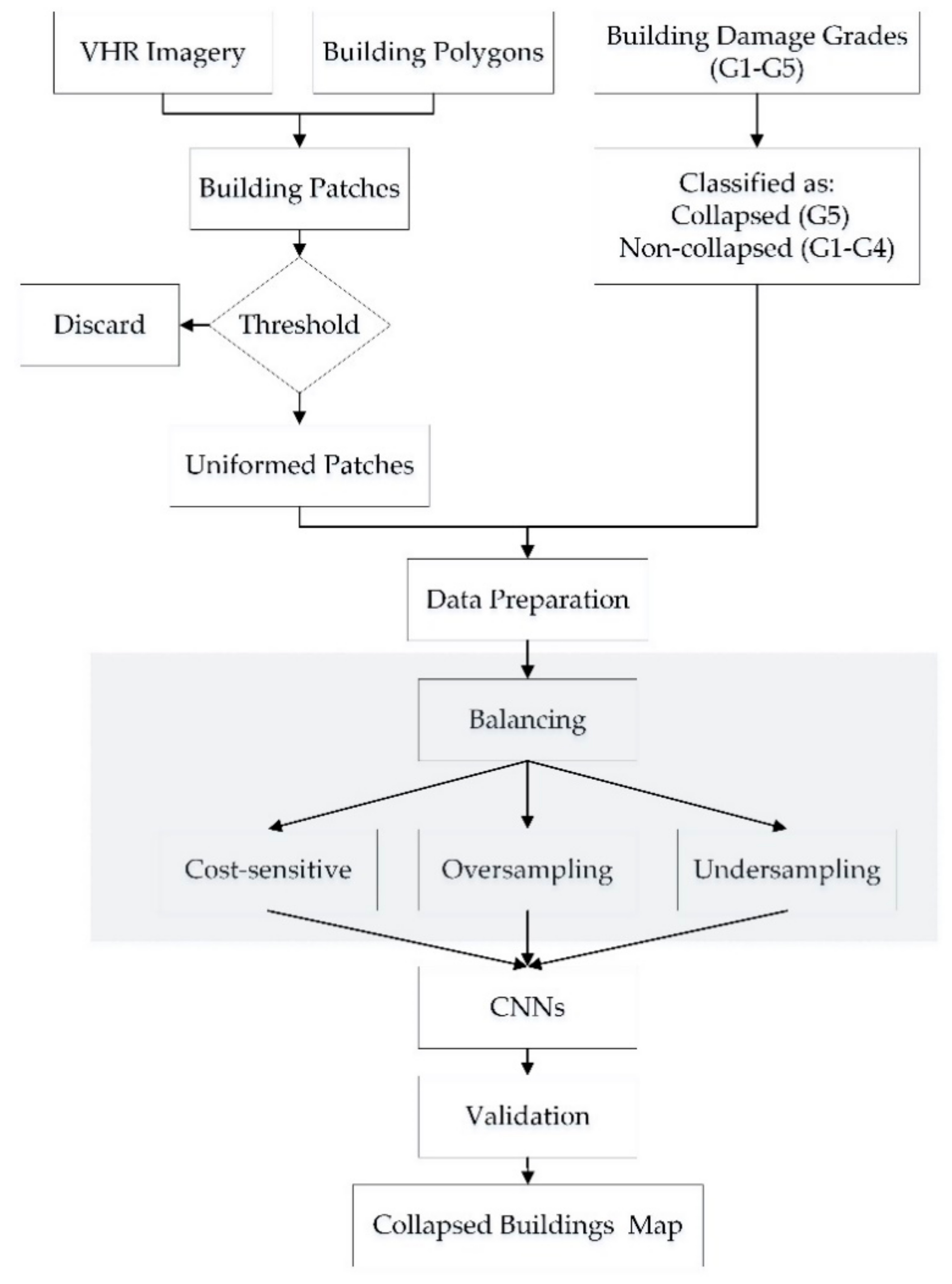
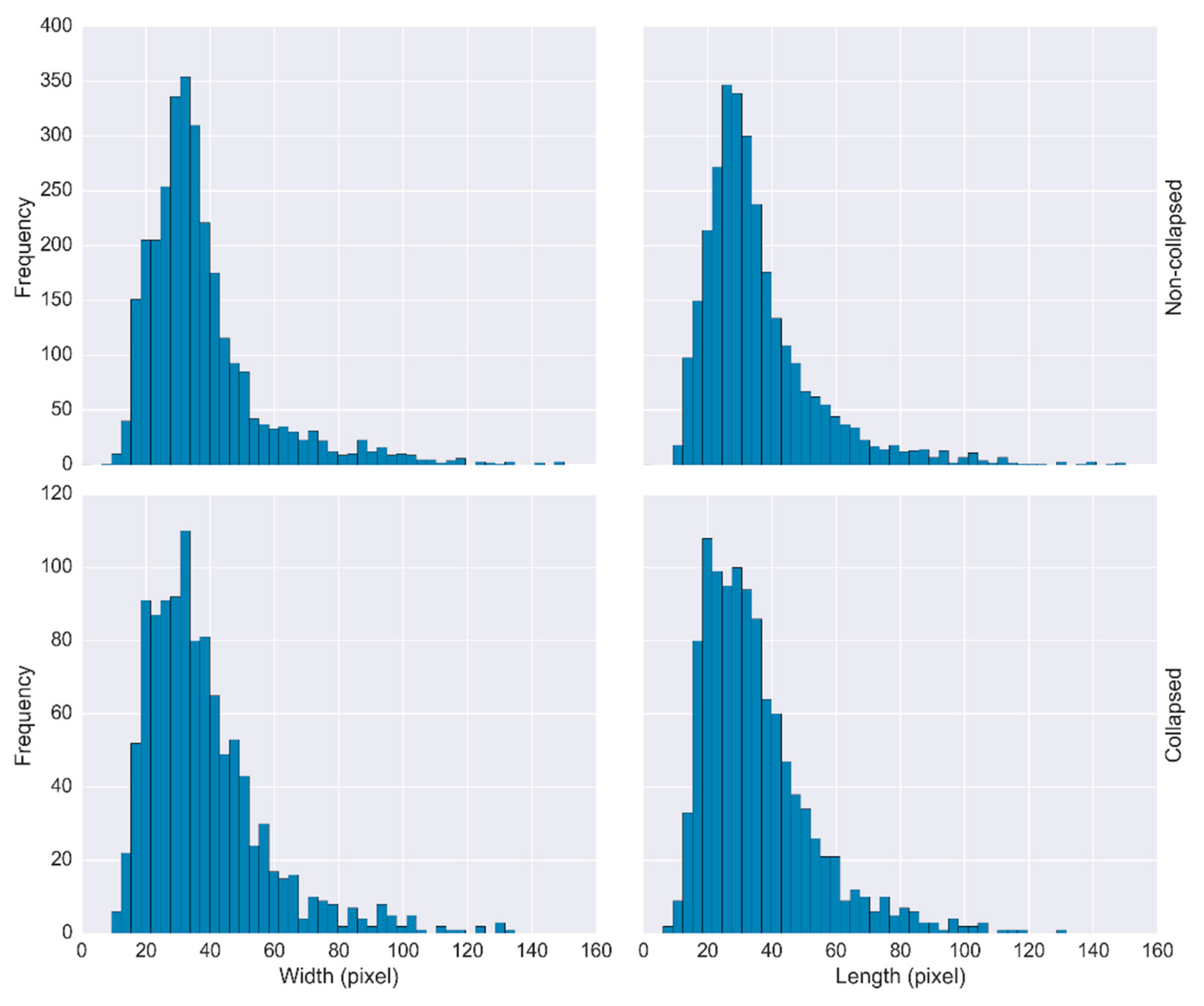
2. Input Data
3. Methodology
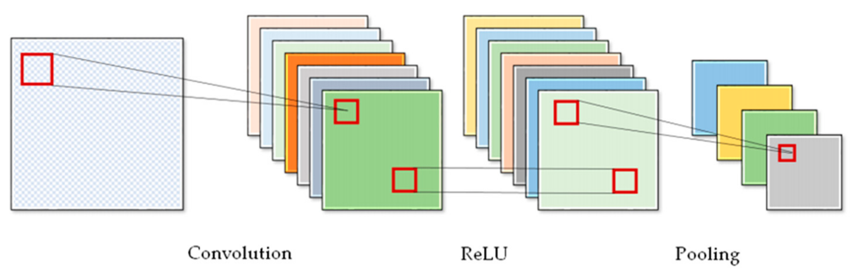
3.1. Convolutional Neural Networks (CNNs)
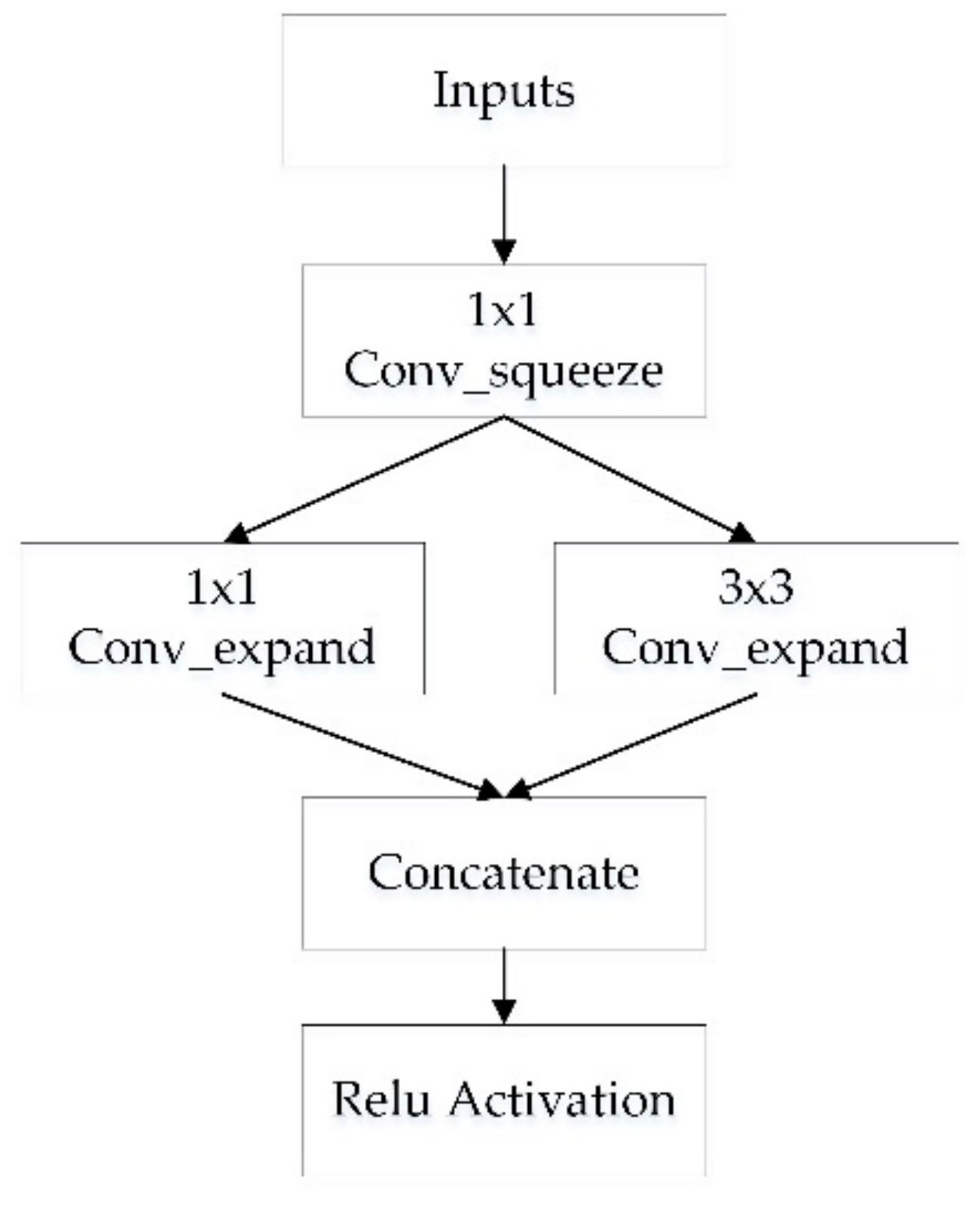
3.2. SqueezeNet
3.3. Data Balancing Methods
3.4. Evaluation Metrics
4. Results and Discussion
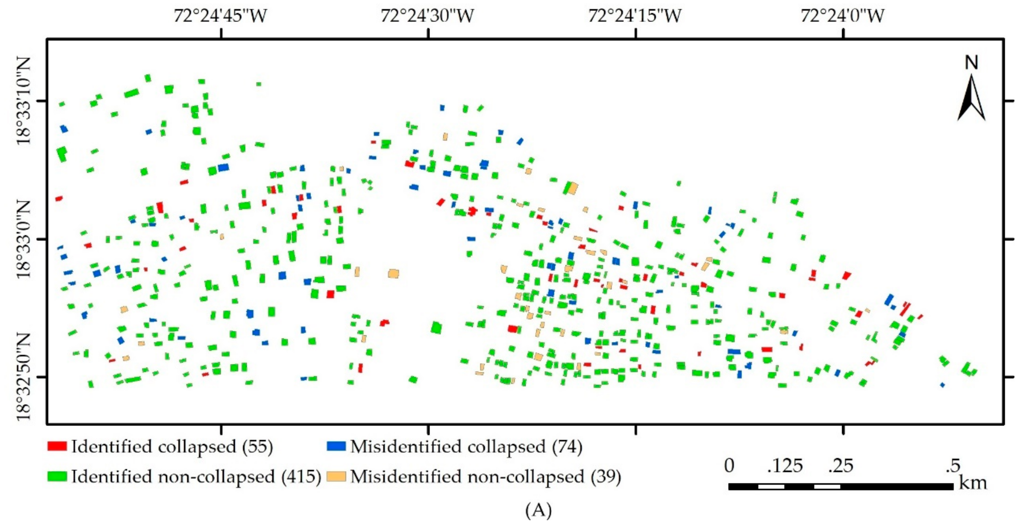
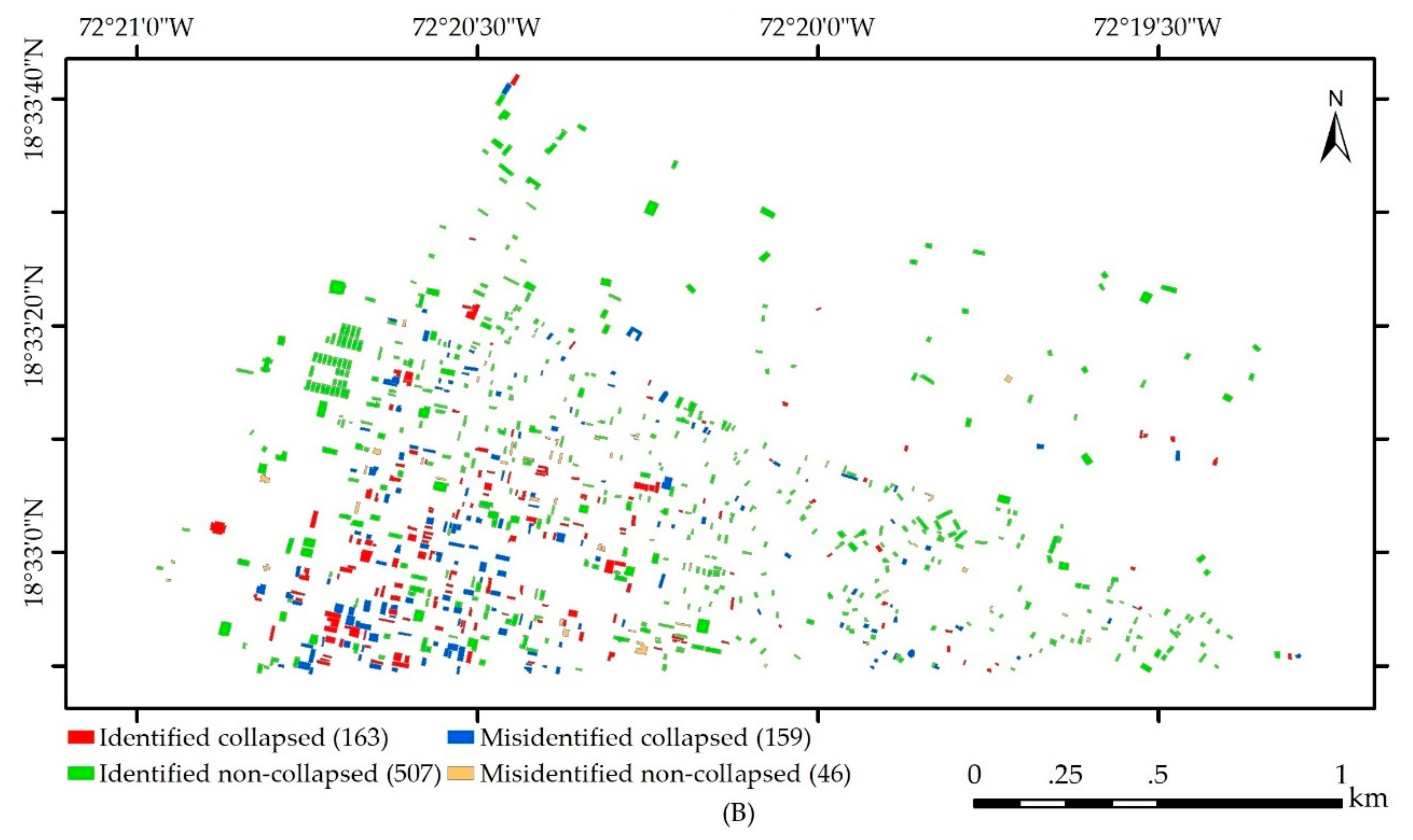
4.1. Identifying Collapsed Buildings Using CNNs
4.2. Performance of Balancing Methods for Identifying Collapsed Buildings
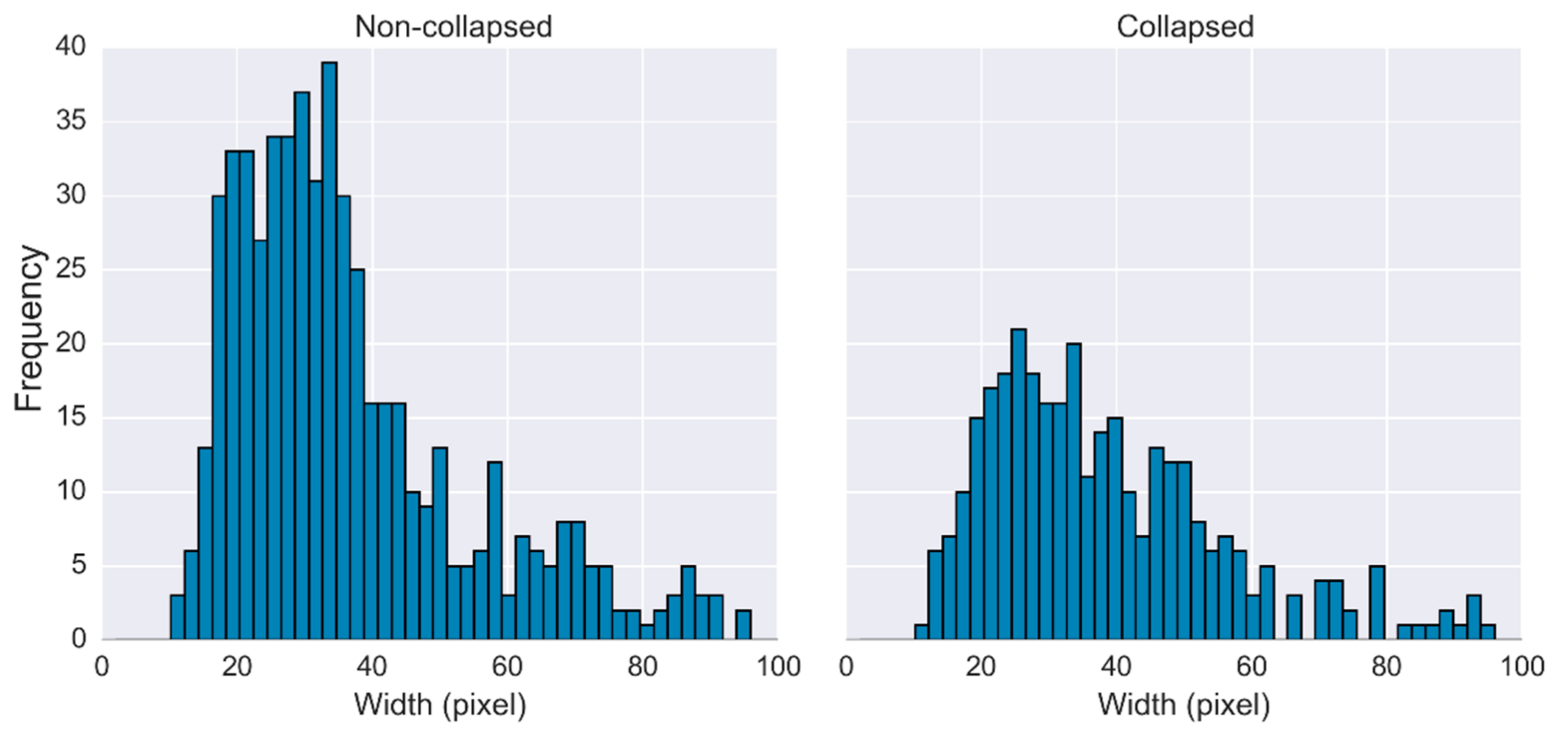
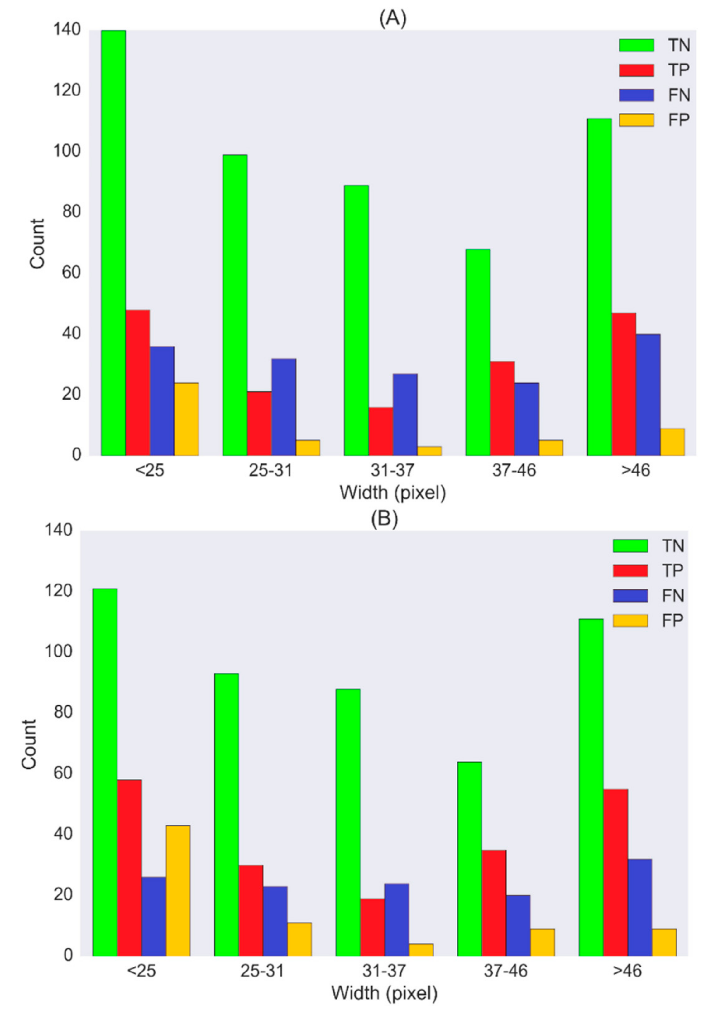
4.3. Intra-Class Analysis for Building Damage Assessment
4.4. CNNs for Identifying Earthquake-Induced Collapsed Buildings
5. Conclusions
Author Contributions
Funding
Acknowledgments
Conflicts of Interest
References
- Cooner, A.J.; Shao, Y.; Campbell, J.B. Detection of urban damage using remote sensing and machine learning algorithms: Revisiting the 2010 Haiti earthquake. Remote Sens. 2016, 8, 868. [Google Scholar] [CrossRef]
- Uprety, P.; Yamazaki, F.; Dell’Acqua, F. Damage detection using high-resolution SAR imagery in the 2009 L’Aquila, Italy, earthquake. Earthq. Spectra 2013, 29, 1521–1535. [Google Scholar] [CrossRef]
- He, M.; Zhu, Q.; Du, Z.; Hu, H.; Ding, Y.; Chen, M. A 3D shape descriptor based on contour clusters for damaged roof detection using airborne LiDAR point clouds. Remote Sens. 2016, 8, 189. [Google Scholar] [CrossRef]
- Menderes, A.; Erener, A.; Sarp, G. Automatic detection of damaged buildings after earthquake hazard by using remote sensing and information technologies. Procedia Earth Planet. Sci. 2015, 15, 257–262. [Google Scholar] [CrossRef]
- Ghosh, S.; Huyck, C.K.; Greene, M.; Stuart, P.; Bevington, J.; Svekla, W.; Desroches, R. Crowdsourcing for rapid damage assessment: The global earth observation catastrophe assessment network (GEO-CAN). Earthq. Spectra 2011, 27, S179–S198. [Google Scholar] [CrossRef]
- Corbane, C.; Saito, K.; Oro, L.D.; Bjorgo, E.; Gill, S.P.D.; Piard, B.E.; Huyck, C.K.; Kemper, T.; Lemoine, G.; Spence, R.J.S.; et al. A comprehensive analysis of building damage in the 12 January 2010 Mw 7 Haiti earthquake using high-resolution satellite-and aerial imagery. Photogramm. Eng. Remote Sens. 2011, 77, 997–1009. [Google Scholar] [CrossRef]
- Gokon, H.; Koshimura, S. Mapping of building damage of the 2011 Tohoku earthquake tsunami in Miyagi Prefecture. Coast. Eng. J. 2012, 54, 1250006. [Google Scholar] [CrossRef]
- Dong, L.; Shan, J. A comprehensive review of earthquake-induced building damage detection with remote sensing techniques. ISPRS J. Photogramm. Remote Sens. 2013, 84, 85–99. [Google Scholar] [CrossRef]
- Saito, K.; Spence, R. Rapid damage mapping using post-earthquake satellite images. In Proceedings of the 2004 IEEE International Geoscience and Remote Sensing Symposium, Anchorage, AK, USA, 20–24 September 2004; Volume 4, pp. 2272–2275. [Google Scholar]
- Rathje, E.M.; Crawford, M.; Woo, K.; Neuenschwander, A. Damage patterns from satellite images of the 2003 Bam, Iran, earthquake. Earthq. Spectra 2005, 21, 295–307. [Google Scholar] [CrossRef]
- Turker, M.; Sumer, E. Building-based damage detection due to earthquake using the watershed segmentation of the post-event aerial images. Int. J. Remote Sens. 2008, 29, 3073–3089. [Google Scholar] [CrossRef]
- Mitomi, H.; Saita, J.; Matsuoka, M.; Yamazaki, F. Automated damage detection of buildings from aerial television images of the 2001 Gujarat, India earthquake. In Proceedings of the IEEE 2001 International Geoscience and Remote Sensing Symposium (IGARSS 2001), Sydney, NSW, Australia, 9–13 July 2001; Volume 1, pp. 147–149. [Google Scholar]
- Aoki, H.; Matsuoka, M.; Yamazaki, F. Automated detection of damaged buildings due to earthquakes using aerial HDTV and photographs. J. Jpn. Soc. Photogramm. Remote Sens. 2001, 40, 27–36. [Google Scholar] [CrossRef]
- Brunner, D.; Lemoine, G.; Bruzzone, L. Earthquake damage assessment of buildings using VHR optical and SAR imagery. IEEE Trans. Geosci. Remote Sens. 2010, 48, 2403–2420. [Google Scholar] [CrossRef]
- Park, S.E.; Yamaguchi, Y.; Kim, D.J. Polarimetric SAR remote sensing of the 2011 Tohoku earthquake using ALOS/PALSAR. Remote Sens. Environ. 2013, 132, 212–220. [Google Scholar] [CrossRef]
- Zhai, W.; Shen, H.F.; Huang, C.L.; Pei, W.S. Building damage information investigation after earthquake using single post-event polsar image. In Proceedings of the 2016 IEEE International Geoscience and Remote Sensing Symposium (IGARSS), Beijing, China, 10–15 July 2016; pp. 7338–7341. [Google Scholar]
- Shi, L.; Sun, W.; Yang, J.; Li, P.; Lu, L. Building collapse assessment by the use of postearthquake Chinese VHR airborne SAR. IEEE Geosci. Remote Sens. Lett. 2015, 12, 2021–2025. [Google Scholar] [CrossRef]
- Timo, B.; Liao, M. Building-damage detection using post-seismic high-resolution SAR satellite data. Int. J. Remote Sens. 2010, 31, 3369–3391. [Google Scholar]
- Zhai, W.; Huang, C. Fast building damage mapping using a single post-earthquake PolSAR image: A case study of the 2010 Yushu earthquake. Earth Planets Space 2016, 68, 86. [Google Scholar] [CrossRef]
- Rastiveis, H.; Eslamizade, F.; Hosseini-Zirdoo, E. Building damage assessment after earthquake using post-event LiDAR data. Int. Arch. Photogramm. Remote Sens. Spat. Inf. Sci. 2015, 40, 595. [Google Scholar] [CrossRef]
- Labiak, R.C.; Van Aardt, J.A.N.; Bespalov, D.; Eychner, D.; Wirch, E.; Bischof, H.-P. Automated method for detection and quantification of building damage and debris using post-disaster lidar data. In Proceedings of the Laser Radar Technology and Applications XVI, Orlando, FL, USA, 25–29 April 2011; Article No; Volume 8037. [Google Scholar]
- Dou, X.; Ma, Z.; Huang, S.; Wang, X. Building damage extraction from post-earthquake airborne LiDAR data. Acta Geol. Sin. (Engl. Ed.) 2016, 90, 1481–1489. [Google Scholar]
- Yu, H.; Mohammed, M.A.; Mohammadi, M.E.; Moaveni, B.; Barbosa, A.R.; Stavridis, A.; Wood, R.L. Structural identification of an 18-story RC building in Nepal using post-earthquake ambient vibration and Lidar data. Front. Built Environ. 2017, 3. [Google Scholar] [CrossRef]
- Wu, F.; Gong, L.; Wang, C.; Member, S.; Zhang, H. Signature analysis of building damage with TerraSAR-X new staring spotLight mode data. IEEE Geosci. Remote Sens. Lett. 2016, 13, 1696–1700. [Google Scholar] [CrossRef]
- Li, X.W.; Guo, H.D.; Zhang, L.; Chen, X.; Liang, L. A new approach to collapsed building extraction using RADARSAT-2 polarimetric SAR imagery. IEEE Geosci. Remote Sens. Lett. 2012, 9, 677–681. [Google Scholar]
- Tong, X.; Hong, Z.; Liu, S.; Zhang, X.; Xie, H.; Li, Z.; Yang, S.; Wang, W.; Bao, F. Building-damage detection using pre-and post-seismic high-resolution satellite stereo imagery: A case study of the May 2008 Wenchuan earthquake. ISPRS J. Photogramm. Remote Sens. 2012, 68, 13–27. [Google Scholar] [CrossRef]
- Rastiveis, H.; Samadzadegan, F.; Reinartz, P. A fuzzy decision making system for building damage map creation using high resolution satellite imagery. Nat. Hazards Earth Syst. Sci. 2013, 13, 455. [Google Scholar] [CrossRef] [Green Version]
- Batista, G.E.; Carvalho, A.C.; Monard, M.C. Applying one-sided selection to unbalanced datasets. In Proceedings of the Mexican International Conference on Artificial Intelligence, Acapulco, Mexico, 11–14 April 2000; Springer: Berlin/Heidelberg, Germany, 2000. [Google Scholar]
- Li, L.; Li, Z.; Zhang, R.; Ma, J.; Lei, L. Collapsed buildings extraction using morphological profiles and texture statistics—A case study in the 5.12 Wenchuan earthquake. In Proceedings of the 2010 IEEE International Geoscience and Remote Sensing Symposium, Honolulu, HI, USA, 25–30 July 2010; pp. 2000–2002. [Google Scholar]
- Yu, H.; Cheng, G.; Ge, X. Earthquake-collapsed building extraction from LiDAR and aerophotograph based on OBIA. In Proceedings of the 2nd International Conference on Information Science and Engineering, Hangzhou, China, 4–6 December 2010; pp. 2034–2037. [Google Scholar]
- Taskin Kaya, G.; Musaoglu, N.; Ersoy, O.K. Damage assessment of 2010 Haiti earthquake with post-earthquake satellite image by support vector selection and adaptation. Photogramm. Eng. Remote Sens. 2011, 77, 1025–1035. [Google Scholar] [CrossRef]
- Bialas, J.; Oommen, T.; Rebbapragada, U.; Levin, E. Object-based classification of earthquake damage from high-resolution optical imagery using machine learning. J. Appl. Remote Sens. 2016, 10, 036025. [Google Scholar] [CrossRef]
- Gong, L.; Wang, C.; Wu, F.; Zhang, J.; Zhang, H.; Li, Q. Earthquake-induced building damage detection with post-event sub-meter VHR TerraSAR-X staring spotlight imagery. Remote Sens. 2016, 8, 887. [Google Scholar] [CrossRef]
- LeCun, Y.; Bengio, Y. Convolutional networks for images, speech, and time-series. In The Handbook of Brain Theory and Neural Networks; MIT Press: Cambridge, MA, USA, 1995; Volume 3361. [Google Scholar]
- Bengio, Y.; Haffner, P. Gradient-based learning applied to document recognition. Proc. IEEE 1998, 86, 2278–2324. [Google Scholar] [Green Version]
- Liu, L.; Ji, M.; Buchroithner, M. Transfer learning for soil spectroscopy based on convolutional neural networks and its application in soil clay content mapping using hyperspectral imagery. Sensors 2018, 18, 3169. [Google Scholar] [CrossRef] [PubMed]
- Krizhevsky, A.; Hinton, G.E. ImageNet classification with deep convolutional neural networks. In Proceedings of the 25th International Conference on Neural Information Processing Systems, Lake Tahoe, NV, USA, 3–6 December 2012; pp. 1097–1105. [Google Scholar]
- Simonyan, K.; Zisserman, A. Very deep convolutional networks for large-scale image recognition. In Proceedings of the International Conference on Learning Representations, San Diego, CA, USA, 7–9 May 2015. [Google Scholar]
- Szegedy, C.; Liu, W.; Jia, Y.; Sermanet, P.; Reed, S.; Anguelov, D.; Erhan, D.; Vanhoucke, V.; Rabinovich, A. Going deeper with convolutions. In Proceedings of the IEEE Conference on Computer Vision and Pattern Recognition, Boston, MA, USA, 7–12 June 2015; pp. 1–9. [Google Scholar]
- Iandola, F.N.; Han, S.; Moskewicz, M.W.; Ashraf, K.; Dally, W.J.; Keutzer, K. SqueezeNet: AlexNet-level accuracy with 50x fewer parameters and <0.5 MB model size. arXiv, 2016; arXiv:1602.07360. [Google Scholar]
- Bai, Y.; Gao, C.; Singh, S.; Koch, M.; Adriano, B.; Mas, E.; Koshimura, S. A framework of rapid regional tsunami damage recognition from post-event terraSAR-X imagery using deep neural networks. IEEE Geosci. Remote Sens. Lett. 2018, 15, 43–47. [Google Scholar] [CrossRef]
- Vetrivel, A.; Gerke, M.; Kerle, N.; Nex, F.; Vosselman, G. Disaster damage detection through synergistic use of deep learning and 3D point cloud features derived from very high resolution oblique aerial images, and multiple-kernel-learning. ISPRS J. Photogramm. Remote Sens. 2018, 140, 45–59. [Google Scholar] [CrossRef]
- Zhang, X.; Song, Q.; Zheng, Y.; Hou, B.; Gou, S. Classification of imbalanced hyperspectral imagery data using support vector sampling. In Proceedings of the 2014 IEEE Geoscience and Remote Sensing Symposium, Quebec City, QC, Canada, 13–18 July 2014; pp. 2870–2873. [Google Scholar]
- Puertas, O.L.; Brenning, A.; Meza, F.J. Balancing misclassification errors of land cover classification maps using support vector machines and Landsat imagery in the Maipo river basin (Central Chile, 1975–2010). Remote Sens. Environ. 2013, 137, 112–123. [Google Scholar] [CrossRef]
- Syafiq, M.; Pozi, M.; Sulaiman, N.; Mustapha, N. A new classification model for a class imbalanced data set using genetic programming and support vector machines: Case study for wilt disease classification. Remote Sens. Lett. 2015, 6, 568–577. [Google Scholar]
- Owen, A.B. Infinitely imbalanced logistic regression. J. Mach. Learn. Res. 2007, 8, 761–773. [Google Scholar]
- Provost, F. Machine learning for the detection of oil spills in satellite radar images. Mach. Learn. 1998, 30, 195–215. [Google Scholar] [CrossRef]
- Buda, M.; Maki, A.; Mazurowski, M.A. A systematic study of the class imbalance problem in convolutional neural networks. Neural Netw. 2018, 106, 249–259. [Google Scholar] [CrossRef] [PubMed]
- Miura, H.; Midorikawa, S.; Matsuoka, M. Building damage assessment using high-resolution satellite SAR images of the 2010 Haiti earthquake. Earthq. Spectra 2016, 32, 591–610. [Google Scholar] [CrossRef]
- UNITAR/UNOSAT; EC Joint Research Centre; World Bank. Haiti Earthquake 2010: Remote Sensing Damage Assessment. Available online: http://www.unitar.org/unosat/haiti-earthquake-2010-remote-sensing-based-building-damage-assessment-data (accessed on 10 May 2017).
- Grünthal, G. European Macroseismic Scale 1998; Cahiers du Centre Europèen de Gèodynamique et de Seismologie, Conseil de l’Europe, Ed.; Centre Europèen de Géodynamique et de Séismologie: Luxembourg, 1998. [Google Scholar]
- Huang, B.; Zhao, B.; Song, Y. Urban land-use mapping using a deep convolutional neural network with high spatial resolution multispectral remote sensing imagery. Remote Sens. Environ. 2018, 214, 73–86. [Google Scholar] [CrossRef]
- Ferreira, A.; Giraldi, G. Convolutional neural network approaches to granite tiles classification. Expert Syst. Appl. 2017, 84, 1–11. [Google Scholar] [CrossRef]
- Guidici, D.; Clark, M. One-dimensional convolutional neural network land-cover classification of multi-seasonal hyperspectral imagery in the San Francisco Bay Area, California. Remote Sens. 2017, 9, 629. [Google Scholar] [CrossRef]
- Sameen, M.I.; Pradhan, B.; Aziz, O.S. Classification of very high resolution aerial photos using spectral-spatial convolutional neural networks. J. Sens. 2018, 2018, 7195432. [Google Scholar] [CrossRef]
- Nair, V.; Hinton, G.E. Rectified linear units improve restricted Boltzmann machines. In Proceedings of the 27th International Conference on Machine Learning (ICML10), Haifa, Israel, 21–24 June 2010; pp. 807–814. [Google Scholar]
- Krawczyk, B. Learning from imbalanced data: Open challenges and future directions. Prog. Artif. Intell. 2016, 5, 221–232. [Google Scholar] [CrossRef]
- Hou, Z.H.; Liu, X.Y. On multi-class cost-sensitive learning. Comput. Intell. 2010, 26, 232–257. [Google Scholar]
- Kukar, M.; Kononenko, I. Cost-sensitive learning with neural networks. In Proceedings of the 13th European Conference on Artificial Intelligence, Brighton, UK, 23–28 August 1998; pp. 445–449. [Google Scholar]
- Wozniak, M. Hybrid Classifiers-Methods of Data, Knowledge, and Classifier Combination; Springer: Berlin/Heidelberg, Germany, 2014; Volume 519. [Google Scholar]
- Landis, J.R.; Koch, G.G. The Measurement of Observer Agreement for Categorical Data Published by: International Biometric Society Stable. Biometrics 1977, 33, 159–174. [Google Scholar] [CrossRef] [PubMed]
- Fleet, D.; Hutchison, D. Spatial pyramid pooling in deep convolutional networks for visual recognition. In Proceedings of the European Conference on Computer Vision, Zurich, Switzerland, 6–12 September 2014; Springer: Cham, Switzerland, 2014; pp. 346–361. [Google Scholar]
- Ural, S.; Hussain, E.; Kim, K.; Fu, C.-S.; Shan, J. Building extraction and rubble mapping for city Port-au-Prince post-2010 earthquake with GeoEye-1 imagery and Lidar data. Photogramm. Eng. Remote Sens. 2011, 77, 1011–1023. [Google Scholar] [CrossRef]
- Gao, M.; Hong, X.; Chen, S.; Harris, C.J. A combined SMOTE and PSO based RBF classifier for two-class imbalanced problems. Neurocomputing 2011, 74, 3456–3466. [Google Scholar] [CrossRef]
- Fernández-gómez, M.J.; Asencio-cortés, G.; Troncoso, A.; Martínez-álvarez, F. Large earthquake magnitude prediction in Chile with imbalanced classifiers and ensemble learning. Appl. Sci. 2017, 7, 625. [Google Scholar] [CrossRef]
- Wang, X.; Li, P. Extraction of earthquake-induced collapsed buildings using very high-resolution imagery and airborne lidar data. Int. J. Remote Sens. 2015, 36, 2163–2183. [Google Scholar] [CrossRef]
- Tong, X.; Lin, X.; Feng, T.; Xie, H.; Liu, S.; Hong, Z.; Chen, P. Use of shadows for detection of earthquake-induced collapsed buildings in high-resolution satellite imagery. ISPRS J. Photogramm. Remote Sens. 2013, 79, 53–67. [Google Scholar] [CrossRef]
- Leichtle, T.; Geiß, C.; Lakes, T.; Taubenböck, H. Class imbalance in unsupervised change detection-A diagnostic analysis from urban remote sensing. Int. J. Appl. Earth Obs. Geoinf. 2017, 60, 83–98. [Google Scholar] [CrossRef]
- Chawla, N.V. Data mining for imbalanced datasets: An overview. In Data Mining and Knowledge Discovery Handbook; Springer: Boston, MA, USA, 2009; pp. 875–886. [Google Scholar]
- Pontius, R.G.; Millones, M. Death to Kappa: Birth of quantity disagreement and allocation disagreement for accuracy assessment. Int. J. Remote Sens. 2011, 32, 4407–4429. [Google Scholar] [CrossRef]
- Nijhawan, R.; Raman, B.; Das, J. Proposed hybrid-classifier ensemble algorithm to map snow cover area. J. Appl. Remote Sens. 2018, 12. [Google Scholar] [CrossRef]
- Gerke, M.; Kerle, N. Automatic structural seismic damage assessment with airborne oblique Pictometry© imagery. Photogramm. Eng. Remote Sens. 2011, 77, 885–898. [Google Scholar] [CrossRef]
- Axel, C.; van Aardt, J. Building damage assessment using airborne lidar. J. Appl. Remote Sens. 2017, 11, 046024. [Google Scholar] [CrossRef]
- Voigt, S.; Schneiderhan, T.; Twele, A.; Gähler, M.; Stein, E.; Mehl, H. Rapid damage assessment and situation mapping: Learning from the 2010 Haiti earthquake. Photogramm. Eng. Remote Sens. 2011, 77, 923–931. [Google Scholar] [CrossRef]
- Zhao, B.; Huang, B.; Zhong, Y. Transfer learning with fully pretrained deep convolution networks for land-use classification. IEEE Geosci. Remote Sens. Lett. 2017, 14, 1436–1440. [Google Scholar] [CrossRef]
- Huang, Z.; Pan, Z.; Lei, B. Transfer learning with deep convolutional neural network for SAR target classification with limited labeled data. Remote Sens. 2017, 9, 907. [Google Scholar] [CrossRef]


| Layer | Shape (N, Width, Length, Bands) | Nr. of Parameters | |
|---|---|---|---|
| Input | (N, 96, 96, 3) | 0 | |
| Conv2D | (N, 47, 47, 64) | 1792 | |
| Relu | (N, 47, 47, 64) | 0 | |
| MaxPooling2D | (N, 23, 23, 64) | 0 | |
| Fire Module | Conv2D_squeeze1 × 1 | (N, 23, 23, 16) | 1040 |
| Relu_squeeze1 × 1 | (N, 23, 23, 16) | 0 | |
| Conv2D_expand1 × 1 | (N, 23, 23, 64) | 1088 | |
| Conv2D_expand3 × 3 | (N, 23, 23, 64) | 9280 | |
| Relu_expand1 × 1 | (N, 23, 23, 64) | 0 | |
| Relu_expand3 × 3 | (N, 23, 23, 64) | 0 | |
| Concatenate | (N, 23, 23, 128) | 0 | |
| MaxPooling2D | (N, 11, 11, 128) | 0 | |
| Fire Module | Conv2D_squeeze1 × 1 | (N, 11, 11, 32) | 4128 |
| Relu_squeeze1 × 1 | (N, 11, 11, 32) | 0 | |
| Conv2D_expand1 × 1 | (N, 11, 11, 128) | 4224 | |
| Conv2D_expand3 × 3 | (N, 11, 11, 128) | 36,992 | |
| Relu_expand1 × 1 | (N, 11, 11, 128) | 0 | |
| Relu_expand3 × 3 | (N, 11, 11, 128) | 0 | |
| Concatenate | (N, 11, 11, 256) | 0 | |
| MaxPooling2D | (N, 5, 5, 256) | 0 | |
| Fire Module | Conv2D_squeeze1 × 1 | (N, 5, 5, 48) | 12,336 |
| Relu_squeeze1 × 1 | (N, 5, 5, 48) | 0 | |
| Conv2D_expand1 × 1 | (N, 5, 5, 192) | 9408 | |
| Conv2D_expand3 × 3 | (N, 5, 5, 192) | 83,136 | |
| Relu_expand1 × 1 | (N, 5, 5, 192) | 0 | |
| Relu_expand3 × 3 | (N, 5, 5, 192) | 0 | |
| Concatenate | (N, 5, 5, 384) | 0 | |
| Dropout | (N, 5, 5, 384) | 0 | |
| Conv2D | (N, 5, 5, 2) | 770 | |
| Relu | (N, 5, 5, 2) | 0 | |
| Global-average-pooling | (N, 2) | 0 | |
| Softmax | (N, 2) | 0 | |
| Total | - | - | 164,194 |
| Ground Truth | ||||
|---|---|---|---|---|
| Collapsed | Non-Collapsed | Total | ||
| Predicted | Collapsed | True Positive (TP) | False Positive (FP) | |
| Non-collapsed | False Negative (FN) | True Negative (TN) | ||
| Total | n | |||
| Ground Truth | |||||||
|---|---|---|---|---|---|---|---|
| Collapsed | Non-Collapsed | UA (%) | OA (%) | Kappa (%) | |||
| Test A | Predicted | Collapsed | 55 | 39 | 58.5 | ||
| Non-collapsed | 74 | 415 | 84.9 | ||||
| PA (%) | 42.6 | 91.4 | |||||
| 80.6 | 37.7 | ||||||
| Predicted | Collapsed | 163 | 46 | 78 | |||
| Test B | Non-collapsed | 159 | 507 | 76.1 | |||
| PA (%) | 50.6 | 91.7 | |||||
| 76.6 | 45.6 | ||||||
| Region | Method | Collapsed | Non-Collapsed | OA (%) | Kappa (%) | ||
|---|---|---|---|---|---|---|---|
| PA (%) | UA (%) | PA (%) | UA (%) | ||||
| Test A | Cost-sensitive | 51.2 | 55.4 | 88.3 | 86.4 | 80.1 | 40.6 |
| Random over-sampling | 49.6 | 53.3 | 87.7 | 86.0 | 79.2 | 38.2 | |
| Random under-sampling | 61.2 | 47.6 | 80.8 | 88.0 | 76.5 | 38.1 | |
| Test B | Cost-sensitive | 61.1 | 72.2 | 86.3 | 79.2 | 77.0 | 48.9 |
| Random over-sampling | 60.9 | 71.7 | 86.1 | 79.1 | 76.8 | 48.5 | |
| Random under-sampling | 69.6 | 65.7 | 78.8 | 81.6 | 75.4 | 47.8 | |
| Width (Pixels) | Nr./Train | Nr./Test B | CNN | Balanced-CNN | ||
|---|---|---|---|---|---|---|
| OA (%) | Kappa (%) | OA (%) | Kappa (%) | |||
| <25 | 515 | 248 | 75.8 | 44.0 | 72.2 | 40.8 |
| 25–31 | 500 | 157 | 76.4 | 39.7 | 78.3 | 48.7 |
| 31–37 | 529 | 135 | 77.7 | 39.8 | 79.2 | 45.4 |
| 37–46 | 456 | 128 | 77.3 | 51.7 | 77.3 | 52.6 |
| >46 | 470 | 207 | 76.3 | 48.9 | 80.2 | 57.8 |
© 2018 by the authors. Licensee MDPI, Basel, Switzerland. This article is an open access article distributed under the terms and conditions of the Creative Commons Attribution (CC BY) license (http://creativecommons.org/licenses/by/4.0/).
Share and Cite
Ji, M.; Liu, L.; Buchroithner, M. Identifying Collapsed Buildings Using Post-Earthquake Satellite Imagery and Convolutional Neural Networks: A Case Study of the 2010 Haiti Earthquake. Remote Sens. 2018, 10, 1689. https://0-doi-org.brum.beds.ac.uk/10.3390/rs10111689
Ji M, Liu L, Buchroithner M. Identifying Collapsed Buildings Using Post-Earthquake Satellite Imagery and Convolutional Neural Networks: A Case Study of the 2010 Haiti Earthquake. Remote Sensing. 2018; 10(11):1689. https://0-doi-org.brum.beds.ac.uk/10.3390/rs10111689
Chicago/Turabian StyleJi, Min, Lanfa Liu, and Manfred Buchroithner. 2018. "Identifying Collapsed Buildings Using Post-Earthquake Satellite Imagery and Convolutional Neural Networks: A Case Study of the 2010 Haiti Earthquake" Remote Sensing 10, no. 11: 1689. https://0-doi-org.brum.beds.ac.uk/10.3390/rs10111689