Estimating Evapotranspiration in a Post-Fire Environment Using Remote Sensing and Machine Learning


Civil, Construction and Environmental Engineering, San Diego State University, San Diego, CA 92182, USA
*
Author to whom correspondence should be addressed.
Remote Sens. 2018, 10(11), 1728; https://0-doi-org.brum.beds.ac.uk/10.3390/rs10111728
Submission received: 10 September 2018
/
Revised: 20 October 2018
/
Accepted: 30 October 2018
/
Published: 2 November 2018
(This article belongs to the Special Issue Advances in the Remote Sensing of Terrestrial Evaporation)
Abstract
:In the hydrological cycle, evapotranspiration (ET) transfers moisture from the land surface to the atmosphere and is sensitive to disturbances such as wildfires. Ground-based pre- and post-fire measurements of ET are often unavailable, limiting the potential to understand the extent of wildfire impacts on the hydrological cycle. This research estimated both pre- and post-fire ET using remotely sensed variables and support vector machine (SVM) methods. Input variables (land surface temperature, modified soil-adjusted vegetation index, normalized difference moisture index, normalized burn ratio, precipitation, potential evapotranspiration, albedo and vegetation types) were used to train and develop 56 combinations that yielded 33 unique SVM models to predict actual ET. The models were trained to predict a spatial ET, the Operational Simplified Surface Energy Balance (SSEBop), for the 2003 Coyote Fire in San Diego, California (USA). The optimal SVM model, SVM-ET6, required six input variables and predicted ET for fifteen years with a root-mean-square error (RMSE) of 8.43 mm/month and a R2 of 0.89. The developed model was transferred and applied to the 2003 Old Fire in San Bernardino, California (USA), where a watershed balance approach was used to validate SVM-ET6 predictions. The annual water balance for ten out of fifteen years was within ±20% of the predicted values. This work demonstrated machine learning as a viable method to create a remotely-sensed estimate with wide applicability for regions with sparse data observations and information. This innovative work demonstrated the potential benefit for land and forest managers to understand and analyze the hydrological cycle of watersheds that experience acute disturbances based on this developed predictive ET model.
1. Introduction
Evapotranspiration (ET) is a critical process in both ecological and hydrological modeling as it accounts for the loss of moisture from biotic and abiotic sources. However, it is arguably the most difficult hydrologic flux to estimate due to the complex interactions between climate, geologic and geographic variables [1,2]. In addition, disturbances such as wildfires have the potential to significantly alter hydrologic processes [3,4,5]. For instance, the changes in vegetation and soil structures can form a hydrophobic layer on the land surface and consequently increase surface runoff. Wildfires are also increasing, especially across the western continental United States [6]. During 2000–2015, anthropogenic climate change was estimated to increase forested area exposed to high fire-season fuel aridity by 75% [7]. Forests experiencing acute or chronic disturbances can contribute to regional and seasonal variability of ET, which can complicate accurate modeling and prediction. A thorough understanding of both pre- and post-disturbed ET patterns, both spatially and temporally, is needed to improve ET estimation, which has significant implications for ecosystem and biological processes [8,9].
Currently, numerous remote sensing-based spatial ET models have been developed with different physical representations and algorithms, providing a range of ET estimates. Some of the widely used models include Surface Energy balance (SEB) [10,11,12], Dual-Source ET [13,14,15] and temperature-vegetation indices (T-VI) models [1,16,17] However, most of these spatial models require intensive manual labor, computational storage and power to estimate ET products spatially and temporally for both small and large domains due to the extents of satellite imagery. Automation and simplifications to process ET products have become more time efficient and minimize operator bias and errors [18,19,20] and a novel application of machine learning was proposed to improve the efficiency of estimating ET.
Machine learning (ML) is a subfield of artificial intelligence that learns from experience to develop predictive models [21]. It decreases the input variables and resources required, yet provides high-level prediction accuracy. This becomes a valuable opportunity to model processes where limited knowledge or data are available for calibrating an appropriate model [22]. In addition, standard statistical methods such as multiple regression are difficult to perform with highly nonlinear problems, making ML a more viable option. For instance, estimating evapotranspiration rates in regions that are prone to wildfires is both hydrologically and ecologically variable. ET is influenced by the availability of moisture, vegetation coverage, seasonal patterns andland surface temperature. Specifically, in environments disturbed by wildfire, vegetative transformation and recovery, altered surface runoff and the storage capacity in soil contribute to nonlinear conditions. The range of nonlinear approaches is too complex for multiple regressions to adequately predict outcomes [23]. In addition, other data-driven models—monthly average models, autoregressive integrated moving average are based on linear concepts—are not well suited for estimating evapotranspiration [24].
To address the nonlinearity of ecohydrologic characteristics, many studies have adopted other modelling tools. Under ML, various methods such as support vector machine (SVM), artificial neural networks (ANN), fuzzy logic, decision trees and reinforcement learning have been investigated [21]. Furthermore, ML has been implemented in the field of hydrology in recent decades to downscale results and improve forecasting and predictions of sediment [22,25,26], rainfall [27,28], runoff [29] and evaporation and evapotranspiration [23,30,31]. Yang et al. [23] utilized SVM regression to estimate AmeriFlux ground-based ET data using remotely sensed variables from 2000–2002. The authors noted a root mean square error (RMSE) of 0.62 mm/day, approximately 23% of the mean observed tower data, with a correlation (R2) of 0.75 [28]; This is comparable to other spatial ET models such as Moderate Resolution Imaging Spectroradiometer (MODIS) Global Evapotranspiration Project (MOD 16), which has an average RMSE of 0.90 mm/day and a R2 of 0.58 [14]). Building upon these previous works, this current research adapts and applies SVM to post-wildfire environments to demonstrate a new technique to estimate ET in disturbed systems with only remotely sensed products.
The strengths and weaknesses of hydrologic modeling are often attributed to the availability of the input variables required. In ungauged or remote regions with minimal research and observations, model development and calibration are challenging due to lack of spatial and temporal data. Remotely sensed variables can provide broad coverage of these areas at reasonable spatial and temporal resolutions. The goal of this research, therefore, is to utilize support vector machine regression and remotely sensed variables to predict actual ET within post-wildfire environments. An available spatial ET product, the Operational Simplified Surface Energy Balance (SSEBop) is utilized as an output variable to train and calibrate an SVM model from 2000–2015. Both pre- and post-fire ET estimates were trained with remotely sensed variables: modified soil-adjusted vegetation index (MSAVI), normalized burn ratio (NBR), normalized difference moisture index (NDMI), precipitation, land surface temperature (LST), albedo and vegetation types. The following is presented: (1) an overview of support vector machine regression, (2) a sensitivity analysis of each variable incorporated in this analysis, (3) the SVM model development and (4) an application of the developed SVM model to show the transability of this method to regions with similar physical and seasonal characteristics.
2. Materials and Methods
2.1. SVM Regression
Support vector machine (SVM) was originally developed to solve two-group classification but has been adopted to also solve regression problems. SVM is more sensitive to the variations in the input variables, even with fewer training datasets [32]. Conceptually, SVM finds data points to separate the dataset as far as possible through transformation to a high dimensional hyperplane, in which the dataset can be solved linearly. The SVM formulation employs a structural risk minimization principle, rather than an empirical risk minimization principle, which always allows SVM to derive a unique solution [33]. The determination of the parameters of an optimal hyperplane in a high dimensionality data space is avoided by using a dual setting in the optimization. Furthermore, the use of kernel functions to map into high dimensional hyperplane can minimize the complexity and estimation error of the model.
To configure SVM, three hyperparameters are required: (1) C is the cost of errors; (2) ε represents the ε-insensitive error band and (3) γ is a kernel function parameter. The C value controls the tradeoff between the complexity of the model and the range of the training error. A smaller C value minimizes the regularization (complexity) and allows a soft margin of the classification, allowing a wider gap to be less over-fit. Subsequently, a higher C value limits the satisfaction on the constraints (loss function) and makes the cost of misclassification high, forcing the model to learn the input data more strictly. The ε term defines a training error and as a result, affects the number of support vectors in the dataset. Lastly, γ depends on the specific kernel function selected. In essence, γ influences the bias and variance of output models. A large γ has a small variance, indicating the support vector has a narrow-spread influence. While a small γ has a larger influence on the classification of the testing values, which avoids overfitting but is not able to capture the complexity of the data. Further detail is included in Appendix A.
2.2. SVM Model Development
2.2.1. Datasets
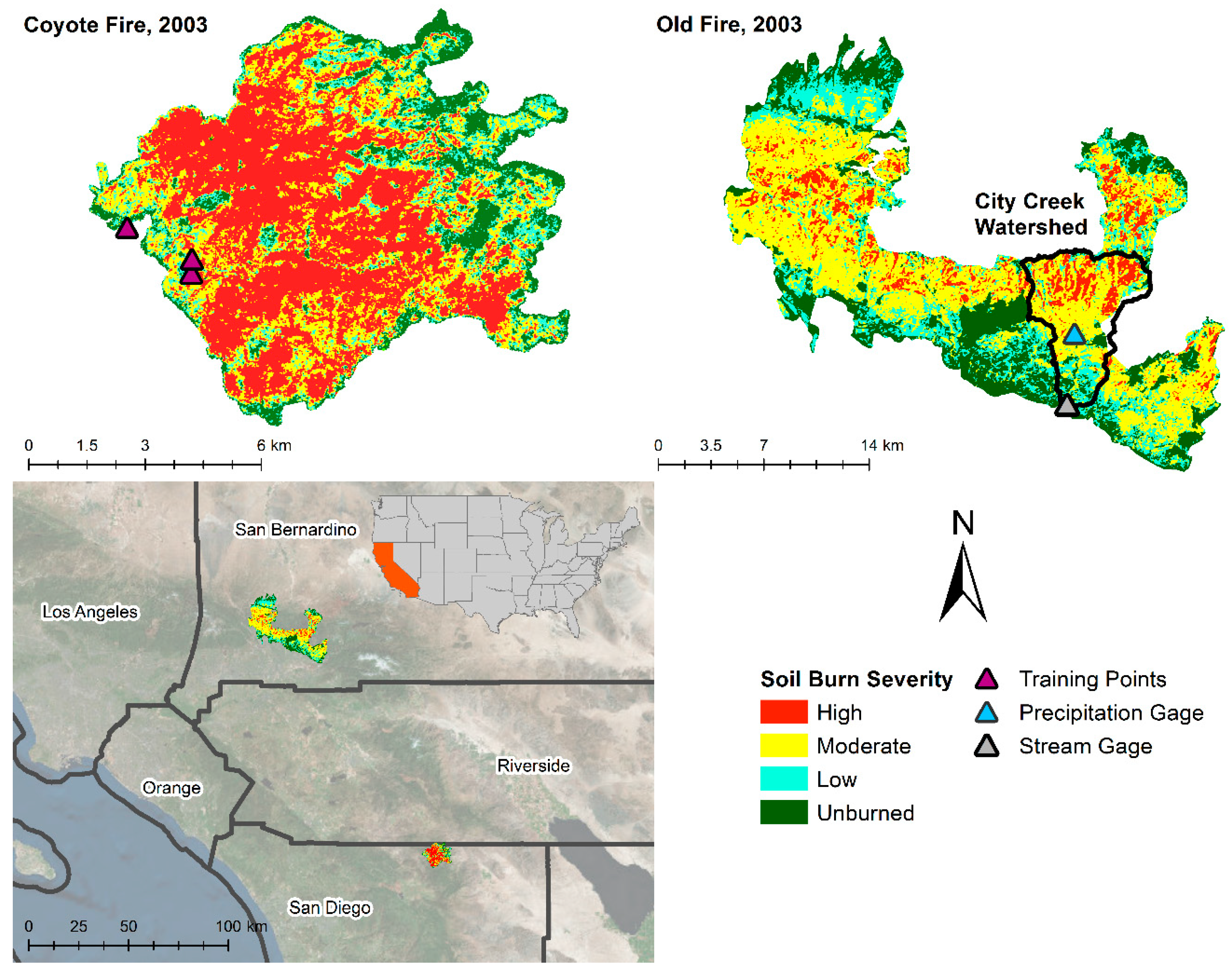
Two sets of data were acquired to perform the SVM analysis (Table 1): (1) input variables for training purposes and (2) spatial ET models as output values. The input and output variables utilized in this study are freely available at reasonable spatial and temporal resolutions for the United States. Two wildfires in Southern California (USA) were used as study sites: (1) the 2003 San Diego Coyote Fire (for training) and (2) the 2003 Old Fire in the San Bernardino Mountains (for application) (Figure 1). The Coyote Fire and Old Fire sites were composed of mostly chaparral and shrub (72–78%) and mixed conifer (20%) [34]. The soil type for both sites were also similar and consisted of clay loam and shallow sandy loam (City Creek) and coarse and fine sandy loam (Coyote Fire). The precipitation regimes were similar for normal years with approximately 381–508 mm per year. For wet years, precipitation increases to approximately 762 mm (Coyote Fire) and 1143 mm per year (City Creek) per year (https://water.weather.gov/precip/).
The spatial and temporal coverage for both training and validation was 1-km monthly from 2000–2015. MSAVI, NDMI, LST, albedo, precipitation and potential ET were extracted from the Google Earth Engine (GEE) platform (Table 1).
Input variables included both remotely sensed indices and modeled meteorological variables (land surface temperature, modified soil-adjusted vegetation index, normalized difference moisture index, normalized burn ratio, precipitation, potential evapotranspiration, albedo and vegetation types). Landsat 5–8 Collection 1 Surface Reflectance data were acquired to calculate MSAVI, NDMI and NBR (1–3). The 16-day cloud-free images were used to extract MSAVI, NDMI, LST, albedo, precipitation and potential ET and averaged to monthly values.
Introduced by Qi et al. [35] MSAVI is a modification to the soil-adjusted vegetation index (SAVI), which was proposed by Huete [36] to improve the normalized difference vegetation index (NDVI) in areas with a high degree of exposed soil surface. MSAVI was used to represent the physical vegetative biomass and calculated as:
where NIR represents the near infrared reflectance band and RED is the red reflectance band.
MSAVI = (2 * NIR + 1 − ((2 * NIR +1)2 − 8 * (NIR − RED))0.5)/2
NDMI was utilized to represent the vegetation liquid water through remote sensing by comparing the near infrared and shortwave infrared 1 (SWR1) reflectance bands:
where SWIR1 represents the shortwave infrared at 1.24 µm wavelengths. Liquid water absorption by vegetation in the red band is negligible and liquid absorption in SWIR1 is weak. Atmospheric aerosol scattering effects in the range of these two bands are minimal. Therefore, NDMI is expected to be sensitive to the liquid water content of vegetation canopies since SWIR1 shares similar vegetation scattering properties as NIR and SWIR is sensitive to liquid water changes [37].
NDMI = (NIR − SWIR1)/(NIR + SWIR1)
NBR can be used for detecting burn scars [36]. This index uses NIR and shortwave infrared 2 (SWIR2) reflectance bands:
where SWIR2 represents shortwave infrared from 2.08–2.35 µm. SWIR2 have been shown to represent non-photosynthetically active wood [38,39]. Since NIR is sensitive to the chlorophyll content of live vegetation, the difference of these two bands is sensitive to the changes in the amount of live green vegetation, moisture content and some soil conditions after fire [40].
NBR = (NIR − SWIR2)/(NIR + SWIR2)
Additionally, meteorological variables including precipitation and potential evapotranspiration were included in the training dataset. Precipitation (PPT) data were acquired from a climate analysis system, Precipitation-elevation Regressions on Independent Slopes Model (PRISM). Factors such as elevation, topographic facet orientation, terrain and coastal proximity are considered to spatially interpolate station data. Monthly, 800-m PRISM PPT data were extracted from the GEE Platform. Potential evapotranspiration (ETo) refers to the amount of water leaving the land surface if there is an unlimited amount of moisture available. Abatzoglout [41] coupled PRISM and the North American Land Data Assimilation System Phase 2 (NLDAS-2) to develop a Gridded Surface Meteorological Dataset (GRIDMET) [41]. Daily 4-km daily ETo estimates were acquired from GRIDMET and aggregated to monthly values for this analysis.
MODIS provides moderate to high resolution earth observations and high-order land products. Land surface temperature (LST) and albedo data were acquired from MODIS, which are significant for evapotranspiration processes. LST affects the photosynthetic activities of vegetation and moisture uptake by the plants. In addition, vapor pressure deficit has a linear relationship with saturated vapor pressure, which is derived from LST [42]. The LST product (MOD11A2.006) was filtered by the daytime quality control (QC) band to acquire daytime data only and averaged to monthly estimates.
Albedo measures the reflectivity of land surface to incoming radiation, which influences surface energy fluxes. Alterations in land surface can increase albedo values, which can decrease evapotranspiration in both plot and region scales [43,44]. However, the magnitude of alteration may be balanced by other subsequent changes such as surface and sky temperatures. Albedo data were extracted from MODIS MCD43A3. The data was filtered by the quality control band (BRDF_Albedo_Band_Mandatory_Quality_shortwave) and averaged to monthly estimates.
Poon and Kinoshita [5] showed that SSEBop ET was able to model spatial ET to evaluate seasonal and annual patterns after wildfire. SSEBop ET is available at 1-km, monthly and was used as the output values for the SVM training process. Based on the Simplified Surface Energy Balance, SSEBop directly uses temperature and the ratio of actual ET to reference ET for alfalfa, known as the evaporative fraction [20]. The temperature estimated for SSEBop have pre-defined hot and cold temperature values for dry surfaces for each 1-km by 1-km domain (a pixel) on a given day of the year to derive the evaporative fraction [18]. SSEBop ET data were acquired from the United States Geological Survey (USGS) Geo Data Portal (https://cida.usgs.gov/gdp/).
2.2.2. SVM Training and Tuning
The San Diego Coyote Fire (Figure 1) was used to train the SVM model from 2000–2015. The developed model was subsequently transferred and applied to City Creek, a watershed in the San Bernardino Mountains, which was burned by the 2003 Old Fire. This work used City Creek to demonstrate the feasibility and transferability of developing an SVM model in similar regions without in situ information. Three SSEBop ET pixels were within the Coyote Fire burned area, which contained a mixture of burn severities for the SVM model to learn to differentiate. The fire started on 16 July 2003 and was contained 8 days later, providing 43 months of pre-fire data. After filtering and aggregating the input variables, a total of 576 months of data were standardized and trained with a k-fold cross-validation of 10.
We followed a previous study by Yang et al. [23], which conducted SVM training from 2000–2002 at 25 sites and tested the model at 19 sites for the year 2003. Their application of a developed model to the same site but a different time period (a new set of independent variables) also used k-fold cross-validation to avoid overfitting from the 2000–2002 dataset [23].We conducted the k-fold validation at the test site (Coyote Fire) to obtain the optimal combination, which was compared with the original output results (SSEBop). The model was calibrated at the testing site (Coyote Fire) using k-fold cross-validation to minimize the over-fitting risk. The data was first partitioned into k-sets, where k = 1 through k and is updated for k iterations (k = 1, 2, 3… k). For an iteration, k, the model learning was supervised using all of the sets except the k-th set and validated using the k-th set. The same procedures were repeated with each iteration of k, until each set was validated at least once. The k-set results were averaged to provide a single estimation on the overall SVM model. Afterwards, we transferred the optimal model to a different site (Old Fire), where new parameters were gathered. This site was selected as it had hydrologic data available to validate our model using a water-balance.
Tuning the hyperparameters was needed to optimize the performance of the SVM model. Radial basis function (RBF) kernel was chosen; specifically, the Gaussian kernels were capable of infinite dimensional feature space, where the kernel parameter was set to 2. The ε-insensitive band was based on the dataset distribution, where one-tenth of the standard deviation using the interquartile range of the response variable was 2.8910. Following Schölkopf et al. [45], the parameter, C, was based on the range of the output values.
With the chosen parameters, inputs and response variable, an optimal SVM model was determined using standard statistical metrics (RMSE and R2) and sensitivity analysis. RMSE measures the averaged difference between the prediction of a model and the actual response values and R2 shows the closeness of model prediction. Therefore, an optimal model minimizes the errors (i.e., an RMSE of 0 has no error) and has a high correlation (i.e., an R2 of 1 is a perfect correlation). Sensitivity analysis was conducted to show the contribution of each input variable to the response (SSEBop) by repeating the training with different combinations of input variables. In this study, each variable was used as an unchanged variable first, then additional variables were appended individually in the order shown in Table 2. There were a total of 56 combinations of input variables, however there were only 33 unique model combinations. Out of the 33 model combinations, we selected the most optimal SVM SSEBop ET model (based on the strict definition of the smallest RMSE and highest R2 described above), which we applied in this study.
2.3. SVM Model Application
Following the SVM training process, the SVM SSEBop ET model was applied to City Creek watershed, which had sufficient data after wildfire for comparison. City Creek is 51 km2 and was burned by the 2003 Old Fire in the San Bernardino Mountains, CA (Figure 1) with the following burn severity classification: 13% high, 57% moderate, 17% low and 13% unburned. To demonstrate the transferability of the developed SVM model, a basin-wide annual water balance was used to compare the SVM SSEBop ET model from 2000–2015, with four years of pre-fire and twelve years of post-fire periods.
∆ [mm/yr] = P − Q − ET − S
Precipitation data (P) were acquired from the San Bernardino County Flood Warning System (Sensor ID 2860); surface runoff data (Q) were from a stream gage at the outfall of the watershed (USGS 11055800); the residual (∆) represented the basin-wide water balance, which included soil moisture storage and infiltration (S) and other uncertainties.
3. Results
3.1. SVM Sensitivity Analysis
Sensitivity analysis was performed to identify the combination of input variables that would provide the best SVM model results. Standard statistics (R2 and RMSE) were used for evaluation. In total, 56 SVM models were developed. Since input variable order is not relevant for the model algorithm, 33 unique model combinations were evaluated (Table 2). The models ranged from combinations of two input variables to seven input variables.
A strict rule of smallest RMSE and highest R2 were used to select a model to demonstrate application to post-fire environments. Although there were several combinations with similar results (i.e., R2 = 0.89 and RMSE = 8.45 mm/month), the optimal combination (R2 = 0.89 and RMSE = 8.43 mm/month) from this methodology utilized six variables: PRISM, MSAVI, NDMI, LST, Albedo and ETo (Table 2). This optimal six-variable model combination (henceforth SVM-ET6) was subsequently transferred and applied to an alternate burned watershed (Section 3.2) for comparison (Section 3.3).
3.2. SVM-ET6 Model Performance and Prediction
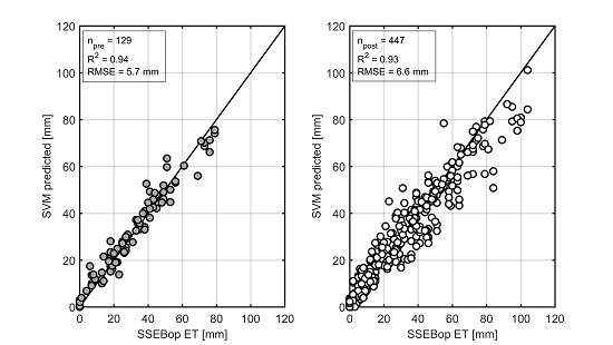
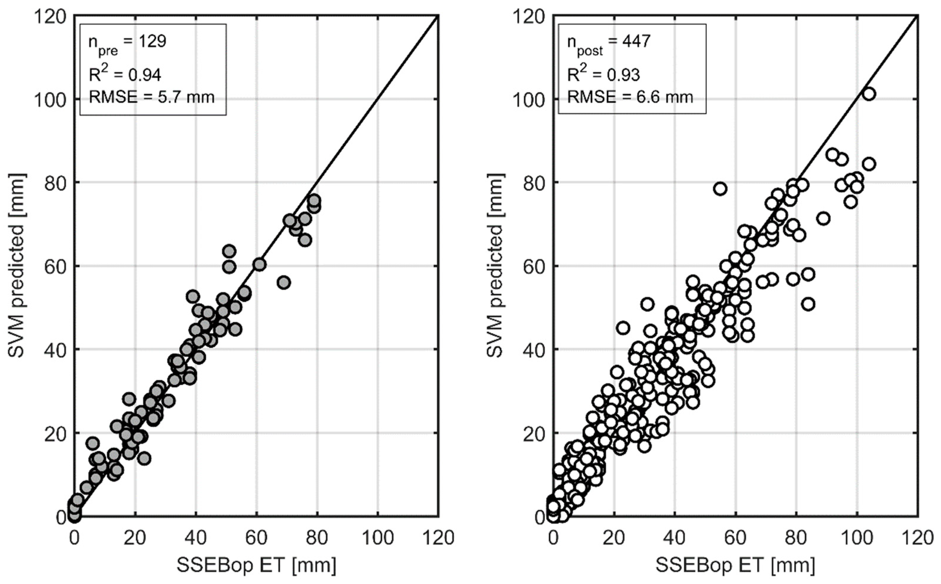
Using the optimal SVM model combination (SVM-ET6) for spatially derived input variables (Section 3.1), the cross-validated results for the Coyote Fire were: R2 = 0.89, RMSE = 8.43 mm/month. For pre-fire months, R2 = 0.94 and RMSE = 5.7 mm/month and post-fire, R2 = 0.93 and RMSE = 6.6 mm/month (Figure 2). These results suggest that using the optimal combination of input variables were able to capture the behavior of the original algorithm of SSEBop ET. To investigate the potential errors of SVM-ET6 estimates, the residual of ET was estimated between SSEBop and SVM-ET6 (actual (SSEBop)—predicted (SVM-ET6); Figure 3). Negative residual (overestimation) occurred at the lower range of ET (10–50 mm) for both pre- and post-fire periods. At the larger range of ET (80–120 mm) during post-fire periods, the residual was between 4–24 mm, indicating that the model did not adequately capture the peaks of post-fire ET. Based on the residual ET, the model performed best from 0–80 mm, with both positive and negative residual values, which indicated no tendencies or bias in the trained model.
3.3. Application of SVM-ET6
This work demonstrated the feasibility of developing an SVM-ET model that can be transferred to regions with similar characteristics. In the current study, vegetation conditions, soil types and precipitation patterns (Section 2.2.1) were comparable. Similarity of hydrologic classification systems such as hydroclimate and soil texture [46] supported the applicability and transferability of SVM-developed models to locations with fewer data resources to obtain meaningful results. We demonstrated a new methodology for remote watersheds or areas with minimal observations. For example, we provided an application of an SVM-ET model to investigate ET after wildfire, where high spatial and temporal resolution information or in situ measurements are typically unavailable.
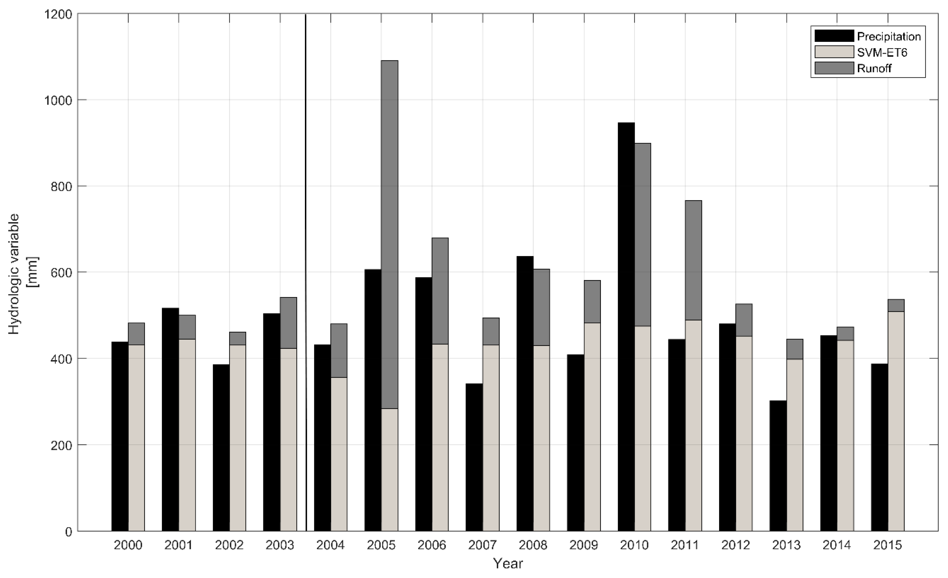
The tuned SVM-ET6 model (Section 3.1) was applied to a watershed in the San Bernardino Mountains, which was burned by the Old Fire in 2003 (Figure 1). The average (μ) precipitation in 2000–2003 (pre-fire) was 461 mm, with a standard deviation (σ) of 60.5 mm, while the runoff average was 64 mm (σ = 38.8 mm). The pre-fire SVM-ET6 had a mean of 433 mm (σ = 9.05 mm; Figure 4). Following the wildfire, the average precipitation during 2004–2007 was 497 mm (σ = 127 mm). The average runoff increased after fire to 310 mm (σ = 340 mm). The average post-fire SVM-ET6 declined to 376 mm (σ = 71.0 mm; Figure 4).
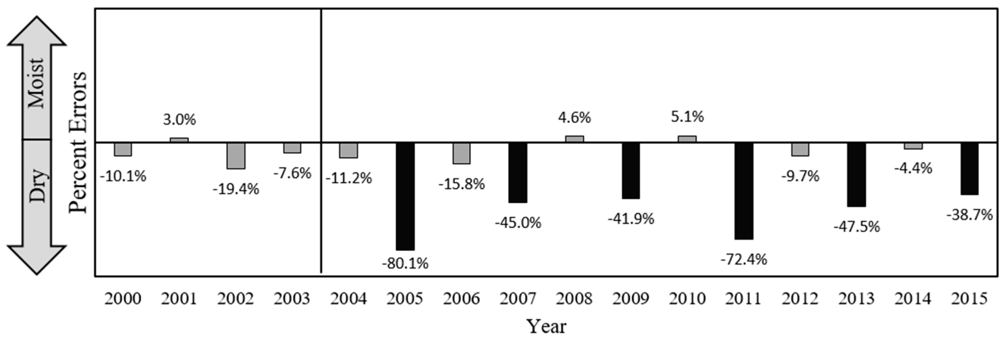
After selecting and training the SVM-ET6 model, City Creek was used to validate the SVM-ET6 estimates with a basin-wide water balance. Based on Equation (4), ∆ should theoretically be 0 due to conservation of mass. A positive ∆ indicates extra moisture on the land surface, whereas a negative ∆ suggests there is extra moisture lost to soil and the atmosphere. The City Creek validation had a total of 10 years within ± 20% (Figure 5).
4. Discussion
4.1. SVM Sensitivity Analysis
The sensitivity analysis suggested that six inputs was the best combination, however, the 33 unique models presented (Table 2) provided an opportunity for additional model options and flexibility. For example, if one of the variables was not readily available for SVM-ET6, an alternate combination, developed with one less variable, such as PRISM, MSAVI, NDMI, LST, could have been used as it provided comparable statistical results (Table 2; R2 = 0.88 and RMSE = 8.74 mm/month). Alternatively, this method can be used to find the most optimal and simplest formulation for modeling post-fire ET. For example, one of the simplest models developed, a two-variable model, consisting of LST as a main input and MSAVI to represent the amount of vegetation within a region. This two variable SVM (LST & MSAVI) model performed relatively well with a correlation of 0.87 with RMSE = 9.04 mm/month; providing a tradeoff between computation and performance. These results conformed to our understanding of land surface temperature and vegetation conditions, which can significantly influence ET. It also highlighted that if the simpler model performs well with less information, then the findings could be more broadly applicable.
In some cases, additional variables were added with minimal statistically-significant improvement (Table 2). Although every input variable was hypothesized to contribute and improve the prediction of ET, the inclusion of EVT uniformly lowered the prediction of ET. This was attributed to the temporal gap within the remotely sensed land cover data (Table 1). The annual EVT dataset (available for 2001, 2008, 2010, 2012 and 2014) was disaggregated to represent monthly conditions throughout 2000–2015. Thus, the actual vegetation type may not have been accurate. For example, the Coyote Fire burned in 2003, however only 2001 and 2008 information was available to represent any potential alteration of vegetation. Considering this limitation, EVT was able to provide reasonable results (R2 = 0.72 and RMSE = 13.3 mm/month) when combined with only MSAVI (Table 2).
We encourage future studies to utilize this methodology to develop ET models using SVM. Prior knowledge of the locations or current understanding of the application (i.e., wildfire responses) can guide the selection of representative and relevant input variables. In the current study, additional variables were incorporated based on previous results by Poon and Kinoshita [5], who noted that decreases in ET varied by burn severity levels (represented by NBR). Similar ground-based studies concluded that burn severity affected the rate of ET following wildfire [47]. Poon and Kinoshita also noted a transformation of vegetation type from conifer to grassland following wildfire, which influenced the rate of ET [5]. Long term evapotranspiration and vegetation changes have also been studied and showed that forested catchments have higher ET rates than grassland [48]. Thus, the current study utilized vegetation as a potential input variable (represented by EVT). NDMI was hypothesized to be an important factor of ET as moisture content contributes to water storage and availability for vegetation processes [49] and baseflow [50]. NBR and EVT did not contribute to the optimal combination (SVM-ET6; Table 2) as expected and NDMI did not show a significant improvement in the model output. Although these input variables provided minimal improvement to the model output in this study, previous literature suggested that these variables were essential to modeling ET. Our observations may have been a function of the burn severity and conditions unique to the study area. On the other hand, LST and MSAVI were also considered relevant variables, which are known to contribute to the moisture and evaporative conditions [16,51]. These input variables showed strong correlation to actual ET rates.
4.2. SVM-ET6 Model Application and Performance
SVM-ET6 decreased by 67 mm and 139 mm, the first and second year following the fire, respectively (Figure 4). This reduction is predominantly due to the loss of vegetation coverage, consequently decreasing transpiration processes and potentially increasing the available soil moisture. Elevated surface runoff was observed two years after the fire, which was attributed to antecedent soil moisture levels [52]. The current research demonstrated that post-fire soil moisture may not have returned to previous conditions prior to the onset of overland flow processes. Thus, approximately 807 mm of additional runoff (650% increase after fire) was observed in 2005 (Figure 4). The t-test for the runoff ratio (runoff/precipitation) and ET ratio (SVM-ET6/precipitation) showed that the pre- and post-fire annual means for both ratios were not statistically different (α > 0.05). This suggests that the altered hydrological processes due to the fire was dominated by soil moisture.
The City Creek validation had a total of 10 years within ±20% (Figure 5). This is within the range observed by Flerchinger and Cooley [53], who conducted a water balance in a semi-arid environment with simulated ET and soil storage estimates. The authors noted that errors ranged from 4–21%, with an average of 10% error (approximately 46 mm). The 20% error margin from the analysis is attributed to limited soil moisture data and information. In the current study, ground-based soil moisture data was not available and spatial soil moisture data had a resolution that was too coarse for City Creek. Considering that City Creek was affected by wildfire, a range of 20% error is reasonable as it falls within the range reported by Flerchinger and Cooley [53].
5. Conclusions
This research is the first to utilize machine learning and remotely sensed indices to develop, train and tune a spatial actual ET model (SVM-ET6) in a semi-arid region prone to wildfires. SVM-ET6 was applied to a burned watershed with similar regional characteristics. A sensitivity analysis of the 33 unique SVM-developed models showed that utilizing PRISM, MSAVI, NDMI, LST, albedo and ETo yielded the most optimal results (R2 = 0.89, RMSE = 8.43 mm/month) and also opportunities for similar results from models with less variables. By coupling remotely sensed variables and machine learning, pre- and post-fire evapotranspiration was predicted and validated using a water balance approach.
We presented methods to leverage support vector machines to produce estimates of evapotranspiration, which can be used to investigate hydrologic processes after disturbance or for circumstances when traditional measurement techniques are often inaccurate or unavailable. This novel application of machine learning in disturbance hydrology also provides a more efficient and accurate representation of ET compared to traditional ground-based methods and models. For regions experiencing acute and chronic disturbances, this is especially critical for understanding water flux partitioning, which can impact biological processes and ecosystem modeling. It also highlights the potential to develop multiple models that can be used to supplement a primary model (such as SVM-ET6 in this case study) to provide ET estimates when site conditions are not optimal or spatial data are unavailable or sparse. Ultimately, this work augments the techniques and tools currently available to managers and researchers for assessing the long-term hydrological cycle after disturbances.
Author Contributions
Conceptualization, P.K.P. and A.M.K.; Data curation, P.K.P.; Formal analysis, P.K.P.; Funding acquisition, P.K.P. and A.M.K.; Investigation, P.K.P.; Methodology, P.K.P.; Project administration, A.M.K.; Resources, A.M.K.; Software, P.K.P.; Supervision, A.M.K.; Visualization, P.K.P.; Writing—original draft, P.K.P. and A.M.K.; Writing—review & editing, P.K.P. and A.M.K.
Funding
This research was supported by NASA Headquarters under the NASA Earth and Space Science Fellowship Program (16-EARTH16F-233).
Acknowledgments
The authors would like to thank the Google Earth Engine community. The authors would also like to thank three anonymous reviewers and the Guest Editors for their reviews.
Conflicts of Interest
The authors declare no conflict of interest. The funders had no role in the design of the study; in the collection, analyses, or interpretation of data; in the writing of the manuscript, or in the decision to publish the results.
Appendix A. Support Vector Machine Regression
Support vector machine (SVM) was originally developed for classification purposes only but the concept can be adopted for regression analysis [54,55]. Since SVM is not the scope of this current work, the algorithm and method discussion only reflect the crucial components of SVM.
The central goal of SVM is to separate and classify datasets by transforming multidimensional space to a new feature space that has higher dimensions, such that the original non-linear problem can be solved linearly.
Consider a set of training data, where xn is a multivariate set of N input data and yn is desirable output response. A general linear relationship is estimated as:
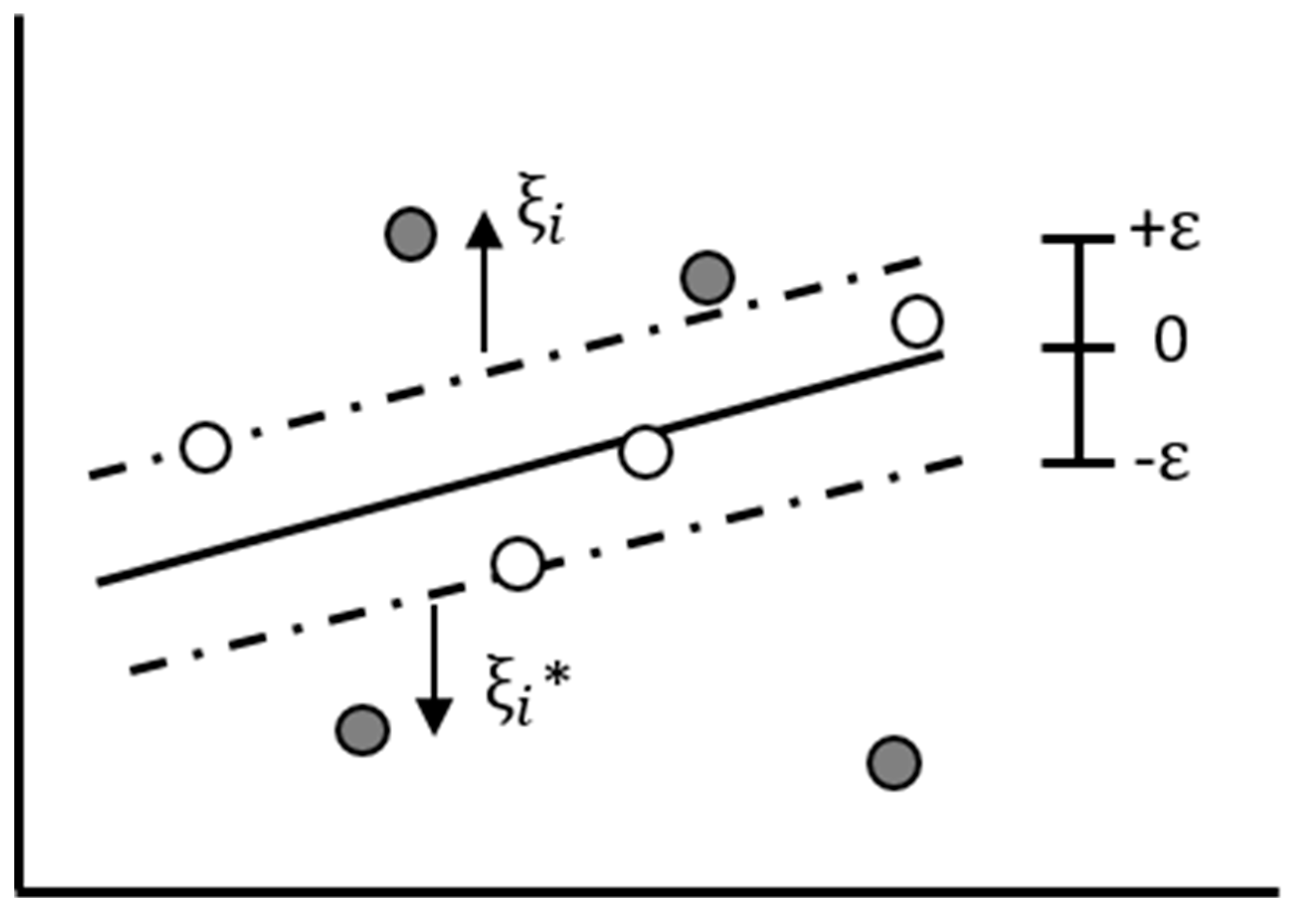
where w represents weight factor and b is constant offset. For a typical classification approach, an optimal plane is found to separate the data as far as possible. In SVM regression, the margin is constructed by using Vapnik’s ε-insensitive loss function ( [54]:
Measured based on the assigned value ε and y (Figure A1), the loss function ignores errors within the margin. The data points that form this boundary are known as support vectors. It is possible that no function can satisfy these constraints for all points, therefore slack variables ( are introduced.
Figure A1.
A desired accuracy ε is specified a priori; Open circles that form the boundary of ε are known as support vectors. Shaded circles indicate two different classes located outside of the margin. The slack variables, ξ, denote the error margin.
Figure A1.
A desired accuracy ε is specified a priori; Open circles that form the boundary of ε are known as support vectors. Shaded circles indicate two different classes located outside of the margin. The slack variables, ξ, denote the error margin.

The concept is similar to the “soft margin” in SVM classification, in which regression errors exist up to the value of both slack variables, yet still satisfy all the conditions. Thus, the primal formula is:
The parameter C controls the model complexity (C is large) and structural risk (C is small) in the optimization formulation.
The minimization with constraints problem can then be solved using Lagrange multipliers. The weight vector is:
To predict new values based on only support vectors, the weight vector is then applied to a linear function:
Lagrange multipliers that are nonzero are called support vectors and provide the solution and other remaining examples (inside the ε band or ) of the training set are irrelevant for contributing to the solution found.
For nonlinear solutions, one replaces xi by mapping into a feature space, (x), to linearize the relation between x and y. Equation (A5) becomes:
Although mapping it to a high-dimension of x is rather difficult, the use of the kernel function can implicitly map the data into a feature space (A6). Most used kernel functions are the Gaussian radial basis function (RBF) with a width of σ and the polynomial kernel. The Gaussian RBF is represented as:
where σ is a priori. Other kernel functions include linear and sigmoid, however RBF is widely used with less computational difficulties and more study cases [23].
In summary, SVM regression transforms a non-linear dataset from a dimensional space to another multi-dimensional space where the dataset is linearly separable. Kernel functions are used to map the higher dimension implicitly.
References
- Kim, J.; Hogue, T.S. Evaluation of a MODIS triangle-based evapotranspiration algorithm for semi-arid regions. J. Appl. Remote Sens. 2013, 7, 73493. [Google Scholar] [CrossRef] [Green Version]
- Xu, C.Y.; Singh, V.P. Evaluation of three complementary relationship evapotranspiration models by water balance approach to estimate actual regional evapotranspiration in different climatic regions. J. Hydrol. 2005, 308, 105–121. [Google Scholar] [CrossRef]
- Ebel, B.A. Simulated unsaturated flow processes after wildfire and interactions with slope aspect. Water Resour. Res. 2013, 49, 8090–8107. [Google Scholar] [CrossRef] [Green Version]
- Bart, R.R. A regional estimate of postfire streamflow change in California. Water Resour. Res. 2016, 52, 1465–1478. [Google Scholar] [CrossRef]
- Poon, P.K.; Kinoshita, A.M. Spatial and temporal evapotranspiration trends after wildfire in semi-arid landscapes. J. Hydrol. 2018, 559, 71–83. [Google Scholar] [CrossRef]
- Westerling, A.L.; Hidalgo, H.G.; Cayan, D.R.; Swetnam, T.W. Warming and earlier spring increase Western U.S. forest wildfire activity. Science 2006, 313, 940–943. [Google Scholar] [CrossRef] [PubMed]
- Abatzoglou, J.T.; Williams, A.P. Impact of anthropogenic climate change on wildfire across western US forests. Proc. Natl. Acad. Sci. USA 2016, 113, 11770–11775. [Google Scholar] [CrossRef] [PubMed] [Green Version]
- Barik, M.G.; Hogue, T.S.; Franz, K.J.; Kinoshita, A.M. Assessing Satellite and Ground-Based Potential Evapotranspiration for Hydrologic Applications in the Colorado River Basin. JAWRA J. Am. Water Resour. Assoc. 2016, 52, 48–66. [Google Scholar] [CrossRef]
- Bowman, A.L.; Franz, K.J.; Hogue, T.S.; Kinoshita, A.M. MODIS-based potential evapotranspiration demand curves for the Sacramento Soil Moisture Accounting model. J. Hydrol. Eng. 2015, 21, 4015055. [Google Scholar] [CrossRef]
- Bastiaanssen, W.G.M.; Menenti, M.; Feddes, R.A.; Holtslagc, A.A.M. A remote sensing surface energy balance algorithm for land (SEBAL). 1. Formulation. J. Hydrol. 1998, 212–213, 213–229. [Google Scholar] [CrossRef]
- Su, Z. The Surface Energy Balance System (SEBS) for estimation of turbulent heat fluxes. Hydrol. Earth Syst. Sci. 2002, 6, 85–100. [Google Scholar] [CrossRef] [Green Version]
- Allen, R.G.; Tasumi, M.; Trezza, R. Satellite-Based Energy Balance for Mapping Evapotranspiration with Internalized Calibration (METRIC)—Model. J. Irrig. Drain. Eng. 2007, 133, 380–394. [Google Scholar] [CrossRef]
- Norman, J.M.; Kustas, W.P.; Humes, K.S. Source approach for estimating soil and vegetation energy fluxes in observations of directional radiometric surface temperature. Agric. For. Meteorol. 1995, 77, 263–293. [Google Scholar] [CrossRef]
- Mu, Q.; Zhao, M.; Running, S.W. Improvements to a MODIS global terrestrial evapotranspiration algorithm. Remote Sens. Environ. 2011, 115, 1781–1800. [Google Scholar] [CrossRef]
- Yang, Y.; Shang, S. A hybrid dual-source scheme and trapezoid framework-based evapotranspiration model (HTEM) using satellite images: Algorithm and model test. J. Geophys. Res. Atmos. 2013, 118, 2284–2300. [Google Scholar] [CrossRef] [Green Version]
- Jiang, L.; Islam, S. An intercomparison of regional latent heat flux estimation using remote sensing data. Int. J. Remote Sens. 2003, 24, 2221–2236. [Google Scholar] [CrossRef]
- Wang, K.; Li, Z.; Cribb, M. Estimation of evaporative fraction from a combination of day and night land surface temperatures and NDVI: A new method to determine the Priestley–Taylor parameter. Remote Sens. Environ. 2006, 102, 293–305. [Google Scholar] [CrossRef]
- Senay, G.B.; Bohms, S.; Singh, R.K.; Gowda, P.H.; Velpuri, N.M.; Alemu, H.; Verdin, J.P. Operational Evapotranspiration Mapping Using Remote Sensing and Weather Datasets: A New Parameterization for the SSEB Approach. J. Am. Water Resour. Assoc. 2013, 49, 577–591. [Google Scholar] [CrossRef]
- Biggs, T.W.; Marshall, M.; Messina, A. Mapping daily and seasonal evapotranspiration from irrigated crops using global climate grids and satellite imagery: Automation and methods comparison. Water Resour. Res. 2016, 52, 7311–7326. [Google Scholar] [CrossRef]
- Bhattarai, N.; Shaw, S.B.; Quackenbush, L.J.; Im, J.; Niraula, R. Evaluating five remote sensing based single-source surface energy balance models for estimating daily evapotranspiration in a humid subtropical climate. Int. J. Appl. Earth Obs. Geoinf. 2016, 49, 75–86. [Google Scholar] [CrossRef]
- Mitchell, T. Machine Learning; McGraw Hill: New York, NY, USA, 1997. [Google Scholar]
- Bhattacharya, B.; Price, R.K.; Solomatine, D.P. Machine learning approach to modeling sediment transport. J. Hydraul. Eng. 2007, 133, 440–450. [Google Scholar] [CrossRef]
- Yang, F.; White, M.A.; Michaelis, A.R.; Ichii, K.; Hashimoto, H.; Votava, P.; Zhu, A.-X.; Nemani, R.R. Prediction of continental-scale evapotranspiration by combining MODIS and AmeriFlux data through support vector machine. IEEE Trans. Geosci. Remote Sens. 2006, 44, 3452–3461. [Google Scholar] [CrossRef]
- Parasuraman, K.; Elshorbagy, A.; Carey, S.K. Modelling the dynamics of the evapotranspiration process using genetic programming. Hydrol. Sci. J. 2007, 52, 563–578. [Google Scholar] [CrossRef] [Green Version]
- Ahmad, S.; Kalra, A.; Stephen, H. Estimating soil moisture using remote sensing data: A machine learning approach. Adv. Water Resour. 2010, 33, 69–80. [Google Scholar] [CrossRef]
- Srivastava, P.K.; Han, D.; Ramirez, M.R.; Islam, T. Machine learning techniques for downscaling SMOS satellite soil moisture using MODIS land surface temperature for hydrological application. Water Resour. Manag. 2013, 27, 3127–3144. [Google Scholar] [CrossRef]
- Hong, W.-C. Rainfall forecasting by technological machine learning models. Appl. Math. Comput. 2008, 200, 41–57. [Google Scholar] [CrossRef]
- Tripathi, S.; Srinivas, V.V.; Nanjundiah, R.S. Downscaling of precipitation for climate change scenarios: A support vector machine approach. J. Hydrol. 2006, 330, 621–640. [Google Scholar] [CrossRef]
- Bray, M.; Han, D. Identification of support vector machines for runoff modelling. J. Hydroinform. 2004, 6, 265–280. [Google Scholar] [CrossRef] [Green Version]
- Jovic, S.; Nedeljkovic, B.; Golubovic, Z.; Kostic, N. Evolutionary algorithm for reference evapotranspiration analysis. Comput. Electron. Agric. 2018, 150, 1–4. [Google Scholar] [CrossRef]
- Torres, A.F.; Walker, W.R.; McKee, M. Forecasting daily potential evapotranspiration using machine learning and limited climatic data. Agric. Water Manag. 2011, 98, 553–562. [Google Scholar] [CrossRef]
- Mohammadrezapour, O.; Piri, J.; Kisi, O. Comparison of SVM, ANFIS and GEP in modeling monthly potential evapotranspiration in an arid region (Case study: Sistan and Baluchestan Province, Iran). Water Sci. Technol. Water Supply 2018. [Google Scholar] [CrossRef]
- Khan, M.S.; Coulibaly, P. Application of support vector machine in lake water level prediction. J. Hydrol. Eng. 2006, 11, 199–205. [Google Scholar] [CrossRef]
- Homer, C.; Huang, C.; Yang, L.; Wylie, B.; Coan, M. Development of a 2001 national land-cover database for the United States. Photogramm. Eng. Remote Sens. 2004, 70, 829–840. [Google Scholar] [CrossRef]
- Qi, J.; Chehbouni, A.; Huete, A.R.; Kerr, Y.H.; Sorooshian, S. A modified soil adjusted vegetation index. Remote Sens. Environ. 1994, 48, 119–126. [Google Scholar] [CrossRef]
- Huete, A.R. A soil-adjusted vegetation index (SAVI). Remote Sens. Environ. 1988, 25, 295–309. [Google Scholar] [CrossRef]
- Gao, B.-C. NDWI—A normalized difference water index for remote sensing of vegetation liquid water from space. Remote Sens. Environ. 1996, 58, 257–266. [Google Scholar] [CrossRef]
- Jia, G.J.; Burke, I.C.; Goetz, A.F.H.; Kaufmann, M.R.; Kindel, B.C. Assessing spatial patterns of forest fuel using AVIRIS data. Remote Sens. Environ. 2006, 102, 318–327. [Google Scholar] [CrossRef]
- Kokaly, R.F.; Rockwell, B.W.; Haire, S.L.; King, T.V.V. Characterization of post-fire surface cover, soils, and burn severity at the Cerro Grande Fire, New Mexico, using hyperspectral and multispectral remote sensing. Remote Sens. Environ. 2007, 106, 305–325. [Google Scholar] [CrossRef]
- Miller, J.D.; Thode, A.E. Quantifying burn severity in a heterogeneous landscape with a relative version of the delta Normalized Burn Ratio (dNBR). Remote Sens. Environ. 2007, 109, 66–80. [Google Scholar] [CrossRef]
- Abatzoglou, J.T. Development of gridded surface meteorological data for ecological applications and modelling. Int. J. Climatol. 2013, 33, 121–131. [Google Scholar] [CrossRef]
- Granger, R.J. Comparison of Surface and Satellite-Derived Estimates of Evapotranspiration Using a Feedback Algorithm. In Proceedings of the 3rd International Workshop on Application of Remote Sensing in Hydrology, NASA Goddard Space Center, Washington, USA, 16–18 October 1996; pp. 71–81. [Google Scholar]
- Israeli, M. The Effect of Soil Surface Condition on the Energy Budget, Soil Temperatures and Evaporation Rate. Ph.D. Thesis, Faculty of Agriculture, Hebrew University of Jerusalem, Jerusalem, Israel, 1966. [Google Scholar]
- Fritschen, L.J. Net and solar radiation relations over irrigated field crops. Agric. Meteorol. 1967, 4, 55–62. [Google Scholar] [CrossRef]
- Schölkopf, B.; Burges, C.J.C.; Smola, A.J. Advances in Kernel Methods: Support Vector Learning; MIT Press: Cambridge, MA, USA, 1999. [Google Scholar]
- Coopersmith, E.J.; Minsker, B.S.; Sivapalan, M. Using similarity of soil texture and hydroclimate to enhance soil moisture estimation. Hydrol. Earth Syst. Sci. 2014, 18, 3095–3107. [Google Scholar] [CrossRef] [Green Version]
- Nolan, R.H.; Lane, P.N.J.; Benyon, R.G.; Bradstock, R.A.; Mitchell, P.J. Changes in evapotranspiration following wildfire in resprouting eucalypt forests. Ecohydrology 2014, 7, 1363–1377. [Google Scholar] [CrossRef]
- Zhang, L.; Dawes, W.R.; Walker, G.R. Response of mean annual evapotranspiration to vegetation changes at catchment scale. Water Resour. Res. 2001, 37, 701–708. [Google Scholar] [CrossRef] [Green Version]
- Atchley, A.L.; Kinoshita, A.M.; Lopez, S.R.; Trader, L.; Middleton, R. Simulating Surface and Subsurface Water Balance Changes Due to Burn Severity. Vadose Zone J. 2018, 17. [Google Scholar] [CrossRef]
- Kinoshita, A.M.; Hogue, T.S. Increased dry season water yield in burned watersheds in Southern California. Environ. Res. Lett. 2015, 10, 14003. [Google Scholar] [CrossRef] [Green Version]
- Knipper, K.R.; Kinoshita, A.M.; Hogue, T.S. Evaluation of a moderate resolution imaging spectroradiometer triangle-based algorithm for evapotranspiration estimates in subalpine regions. J. Appl. Remote Sens. 2016, 10, 016002. [Google Scholar] [CrossRef]
- Kinoshita, A.M.; Hogue, T.S. Spatial and temporal controls on post-fire hydrologic recovery in Southern California watersheds. Catena 2011, 87, 240–252. [Google Scholar] [CrossRef]
- Flerchinger, G.N.; Cooley, K.R. A ten-year water balance of a mountainous semi-arid watershed. J. Hydrol. 2000, 237, 86–99. [Google Scholar] [CrossRef]
- Cortes, C.; Vapnik, V. Support-vector networks. Mach. Learn. 1995, 20, 273–297. [Google Scholar] [CrossRef] [Green Version]
- Vapnik, V. The Nature of Statistical Learning Theory; Springer: New York, NY, USA, 1995. [Google Scholar]
Figure 1.
Two wildfires located in Southern California. The soil burn severity is shown for the 2003 Coyote Fire (used for training and tuning the SVM model at training points) and the 2003 Old Fire (used for SVM-ET6 model application). The City Creek Watershed is delineated within the Old Fire perimeter; precipitation and stream gages are shown.

Figure 2.
Pre- (left) and post-fire (right) SVM-ET6 performance compared to SSEBop ET, where n represents the number of months. A 1:1 ratio is shown as a solid line.
Figure 2.
Pre- (left) and post-fire (right) SVM-ET6 performance compared to SSEBop ET, where n represents the number of months. A 1:1 ratio is shown as a solid line.

Figure 3.
Pre- (left) and post-fire (right) residuals between actual (SSEBop) and predicted (SVM-ET6) ET.
Figure 3.
Pre- (left) and post-fire (right) residuals between actual (SSEBop) and predicted (SVM-ET6) ET.

Figure 4.
Hydrologic variables: annual precipitation (black), SVM-ET6 (light grey) and runoff (dark grey) for City Creek in millimeters. A black solid line separates pre- and post-fire periods.
Figure 4.
Hydrologic variables: annual precipitation (black), SVM-ET6 (light grey) and runoff (dark grey) for City Creek in millimeters. A black solid line separates pre- and post-fire periods.

Figure 5.
The percent errors for the water balance (4) in City Creek. The black solid line separates the pre- and post-fire periods. Grey-filled bars indicate ∆ within the 20% margin of the corresponding year and black-filled bars indicate ∆ outside of the 20% margin. Positive percent errors indicate moist soil conditions, while negative percent errors indicate dry soil conditions.


Table 1.
Input and output variables for SVM. The spatial and temporal resolution and sources are provided.
Table 1.
Input and output variables for SVM. The spatial and temporal resolution and sources are provided.
| Variable Name | Abbreviation | Spatial and Temporal Resolution | Source |
|---|---|---|---|
| Modified soil-adjusted vegetation index * | MSAVI | 30-m; 16 days | Landsat 5, 7 and 8 (Global) |
| Normalized differenced moisture index * | NDMI | 30-m; 16 days | Landsat 5, 7 and 8 (Global) |
| Normalized burn ratio * | NBR | 30-m; 16 days | Landsat 5, 7 and 8 (Global) |
| Parameter-elevation Relationships on Independent Slopes Model precipitation * | PRISM PPT | 800-m; monthly | Oregon State (CONUS) |
| Potential evapotranspiration * | ETo | 4-km; daily | University of Idaho, Gridded Surface Meteorological dataset (CONUS) |
| Land surface temperature * | LST | 1-km; daily | MODIS (Global) |
| Albedo * | Albedo | 500-m; daily | MODIS (Global) |
| Existing vegetation types * | EVT | 30-m; 2001, 2008, 2010, 2012, 2014 | LANDFIRE (CONUS) |
| Operational Surface Energy Balance ^ | SSEBop | 1-km; monthly | United States Geological Survey (CONUS) |
* indicates input variables and ^ represents output values.
Table 2.
Training combinations of input variables and corresponding prediction evaluation statistics (show as R2/RMSE [mm/month]). There are a total of 56 combinations of input variables and 33 unique model combinations +.
Table 2.
Training combinations of input variables and corresponding prediction evaluation statistics (show as R2/RMSE [mm/month]). There are a total of 56 combinations of input variables and 33 unique model combinations +.
| EVT | PRISM | NBR | ETo | Albedo | LST | NDMI | MSAVI | |
|---|---|---|---|---|---|---|---|---|
| MSAVI | 0.72/13.3 | 0.76/12.1 | 0.69/13.8 | 0.80/11.3 | 0.71/13.5 | 0.87/9.04 | 0.72/13.1 | ---- |
| NDMI | 0.73/13.1 | 0.79/11.4 | 0.70/13.8 | 0.81/10.9 | 0.72/13.3 | 0.86/9.23 | ---- | 0.72/13.1 |
| LST | 0.85/9.60 | 0.88/8.74 | 0.87/9.00 | 0.88/8.77 | 0.85/9.70 | ---- | 0.86/9.23 | 0.86/9.23 |
| Albedo | 0.83/10.3 | 0.87/9.00 | 0.87/8.00 | 0.87/9.19 | ---- | 0.85/9.70 | 0.85/9.70 | 0.85/9.70 |
| ETo | 0.85/9.63 | 0.89/8.43 * | 0.88/8.56 | ---- | 0.87/9.20 | 0.87/9.19 | 0.87/9.19 | 0.87/9.19 |
| NBR | 0.86/9.44 | 0.89/8.45 | ---- | 0.86/9.23 | 0.86/9.23 | 0.86/9.23 | 0.86/9.23 | 0.86/9.23 |
| PRISM | 0.88/8.64 | ---- | 0.89/8.45 | 0.89/8.45 | 0.89/8.45 | 0.89/8.45 | 0.89/8.45 | 0.89/8.45 |
| EVT | ---- | 0.88/8.64 | 0.88/8.64 | 0.88/8.64 | 0.88/8.64 | 0.88/8.64 | 0.88/8.64 | 0.88/8.64 |
+ This table is read vertically; each column variable is appended with additional row variable to perform the prediction evaluation. * denotes the optimal combination (SVM-ET6).
© 2018 by the authors. Licensee MDPI, Basel, Switzerland. This article is an open access article distributed under the terms and conditions of the Creative Commons Attribution (CC BY) license (http://creativecommons.org/licenses/by/4.0/).
Share and Cite
MDPI and ACS Style
Poon, P.K.; Kinoshita, A.M. Estimating Evapotranspiration in a Post-Fire Environment Using Remote Sensing and Machine Learning. Remote Sens. 2018, 10, 1728. https://0-doi-org.brum.beds.ac.uk/10.3390/rs10111728
AMA Style
Poon PK, Kinoshita AM. Estimating Evapotranspiration in a Post-Fire Environment Using Remote Sensing and Machine Learning. Remote Sensing. 2018; 10(11):1728. https://0-doi-org.brum.beds.ac.uk/10.3390/rs10111728
Chicago/Turabian StylePoon, Patrick K., and Alicia M. Kinoshita. 2018. "Estimating Evapotranspiration in a Post-Fire Environment Using Remote Sensing and Machine Learning" Remote Sensing 10, no. 11: 1728. https://0-doi-org.brum.beds.ac.uk/10.3390/rs10111728
Note that from the first issue of 2016, this journal uses article numbers instead of page numbers. See further details here.