Radiometric Microwave Indices for Remote Sensing of Land Surfaces


Institute of Applied Physics “Nello Carrara” (IFAC-CNR), via Madonna del Piano, 10, 50019 Firenze, Italy
*
Author to whom correspondence should be addressed.
Remote Sens. 2018, 10(12), 1859; https://0-doi-org.brum.beds.ac.uk/10.3390/rs10121859
Submission received: 10 October 2018
/
Revised: 7 November 2018
/
Accepted: 14 November 2018
/
Published: 22 November 2018
(This article belongs to the Special Issue Microwave Indices from Active and Passive Sensors for Remote Sensing Applications)
Abstract
:This work presents an overview of the potential of microwave indices obtained from multi-frequency/polarization radiometry in detecting the characteristics of land surfaces, in particular soil covered by vegetation or snow and agricultural bare soils. Experimental results obtained with ground-based radiometers on different types of natural surfaces by the Microwave Remote Sensing Group of IFAC-CNR starting from ‘80s, are summarized and interpreted by means of theoretical models. It has been pointed out that, with respect to single frequency/polarization observations, microwave indices revealed a higher sensitivity to some significant parameters, which characterize the hydrological cycle, namely: soil moisture, vegetation biomass and snow depth or snow water equivalent. Electromagnetic models have then been used for simulating brightness temperature and microwave indices from land surfaces. As per vegetation covered soils, the well-known tau-omega (τ-ω) model based on the radiative transfer theory has been used, whereas terrestrial snow cover has been simulated using a multi-layer dense-medium radiative transfer model (DMRT). On the basis of these results, operational inversion algorithms for the retrieval of those hydrological quantities have been successfully implemented using multi-channel data from the microwave radiometric sensors operating from satellite.
1. Introduction
Microwave radiometry has been used since the first space Earth’s observations to investigate some important surface phenomena over the oceans and land at global scale. The early experiments demonstrated that parameters such as ice concentration, wind speed and precipitations over the ocean, as well as some physical characteristics of soil, snow and vegetation can be retrieved at different levels of accuracy and reliability with more or less sophisticated instruments and algorithms developed in several times since the ‘80s. (e.g., [1]).
Further studies have shown that, as expected, combining data collected at different frequencies and polarizations in appropriate indices made it possible to significantly improve the accuracy of the measured quantities, with respect to the one achievable with single frequency/polarization observations. In particular, some Microwave Indices have been successfully related to the main geophysical parameters associated to land hydrological cycle, such as soil moisture (SMC), Plant Water Content (PWC), and Snow Depth (SD) or Snow Water Equivalent (SWE). These indices have therefore been used for implementing operational retrieval algorithms based on data from different channels of satellite radiometric sensors (e.g., SMMR, SSM/I, AMSR-E, AMSR2).
Presently, most of the operational algorithms for monitoring land surfaces are based on visible and infrared indices, such as the Normalized Difference Vegetation Index (NDVI) [2] and Enhanced Vegetation Index (EVI) [3], which is sensitive to vegetation “greenness” and consequently related to its biomass, or the MODIS Snow Cover Fraction. However, observations in optical bands, besides being bound to the light diurnal cycle, are significantly influenced by the presence of clouds and can give information of the observed surface layer only. On the other hand, microwaves are slightly affected by atmospheric perturbations and, depending on the observation frequency and incidence angle, can penetrate in vegetation cover, snow and even the underlying soil. Moreover, the high sensitivity of microwaves to the water content of the observed bodies allows a direct estimate of the SMC, PWC and SWE (e.g., [4,5]).
Investigations on the use of the difference between two linear polarizations for monitoring land surfaces have been carried out since ‘80s by several groups of scientists analyzing passive microwave data from both ground-based and satellite sensors. In particular, a Polarization Index (PI) was defined as the difference between the two linear polarizations (Tbv − Tbh) normalized to their average value [(Tbv + Tbh)/2] [6,7].
As it is well known, the microwave radiation emitted from a specular surface at an angle different from the zenith is partially polarized. The degree of polarization depends on the soil dielectric constant and can be estimated by means of the Fresnel coefficients. When the soil is characterized by a random rough surface the degree of polarization depends on the roughness parameters as well, and decreases as the roughness increases [8]. Moreover, experimental and theoretical investigations have shown that the radiation from a canopy is much less polarized than that from bare soil. The different polarization characteristics of a smooth bare soil and vegetation suggest the possibility of using a polarization measurement, such as PI, as an indicator of vegetation cover.
First studies focused on estimating the sensitivity of the microwave brightness temperature (Tb) to vegetation biomass were carried out since late ‘70s on the basis of ground based experiments and model simulations (e.g., [9,10]) .
The reason for using polarization indices to estimate vegetation biomass was that the measurement at single polarization is influenced by the geometry of plants, providing different results according to the crop type. On the other hand, polarization indices were found to be mostly related to plant water content (PWC) without being significantly influenced by plant structure and surface temperature.
Ref [11], in 1990, identified different combinations of the Special Sensor Microwave Instrument (SSM/I) brightness temperature channels by statistically analyzing satellite data on a global scale, thus allowing the classification of several land classes, such as dense vegetation, rangeland and agricultural soils, deserts, snow, precipitation, and soil surface moisture.
In addition to those based on the polarization difference, other approaches for retrieving PWC from multi-frequency satellite data have been examined combining data at two or more frequencies (e.g., [12]). More recently, [13] noted that the brightness temperatures measured at a given polarization with two adjacent AMSR-E frequency channels can be described by a linear function, which includes two coefficients, both independent of the underlying soil/surface signals and dependent only on vegetation properties. One is positively correlated to NDVI and is affected by the vegetation properties and the surface physical temperature, the other is negatively correlated to NDVI and is only affected by the vegetation properties.
A field of investigations where microwave indices are really useful for implementing retrieval algorithms is the one of snow cover. First investigations on the capability of satellite microwave sensors for snow monitoring took place in early ‘80s by using Nimbus-7 SMMR data over Finland (e.g., [14,15]). Many operative algorithms for the retrieval of the main parameters of snow cover have been implemented since then and are mostly based on multiple combinations of polarizations and frequencies. [16] and [17] developed an operational algorithm for the retrieval of snow depth from SSM/I and AMSR-E data basically using the difference in brightness temperature between Ku and Ka bands in horizontal or vertical polarizations. The Ka band channel is sensitive to scattering by the snowpack while the Ku band channel is relatively unaffected by the snow and is responsive to the surface under the snow [18,19].
Refs [16,20] provided operational algorithms based on microwave indices for their spatial agencies (NASA and JAXA, respectively) focused on the distribution of snow products. In general, the retrieval algorithms are supported by direct theoretical or semi-empirical models, which simulate microwave emission and related indices of land surfaces in different conditions of vegetation, soil moisture, and snow cover. These models are subsequently inverted with greater or lesser success by using different approaches in order to retrieve the main surface parameters.
In this paper, the main results obtained by the Microwave Remote Sensing Group since early 1980s on the retrieval of soil, vegetation and snow parameters using passive microwave data have been reviewed.
2. Experimental Relationships between Microwave Emission and Land Surface Parameters
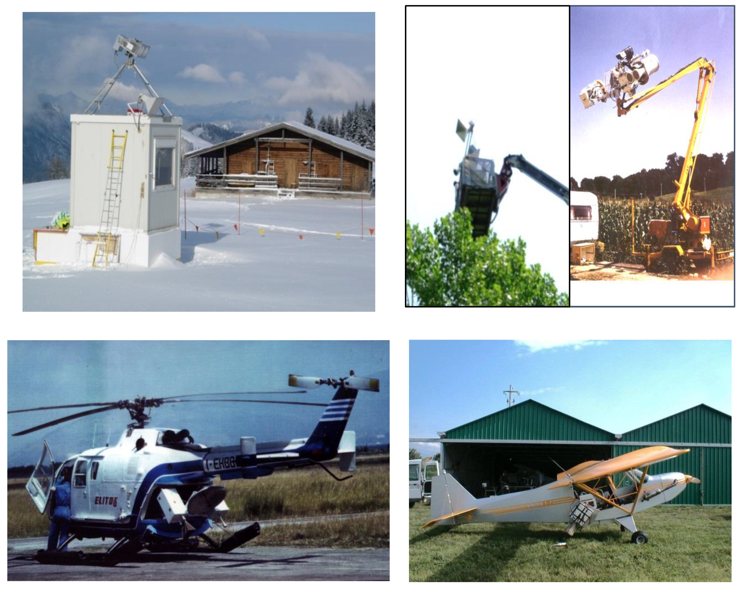
Data presented in this paper were collected on different times and sites from ground-based and airborne platforms by using microwave radiometers, operating at L, C, Ku, and Ka bands in both vertical and horizontal (V&H) polarizations, over bare, vegetated, and snow-covered soils since early ‘80s. Examples of installations of microwave radiometers are shown in Figure 1.
The IFAC microwave instruments were total-power, self-calibrating, dual-polarized radiometers with an internal calibrator based on two loads at different temperatures (cold, 250 K ± 0.2 K, and hot, 370 K ± 0.2 K). The beamwidth of the corrugated conical horns was 20° at −3 dB and 56° at −20 dB for all frequencies and polarizations. Calibration checks were performed during the field experiments by means of absorbing panels of known emissivity and temperature and an internal noise source. Moreover, frequent observations of clear sky were performed. The measurement accuracy (repeatability) was better than ±1 K, with an integration time of 1 s [21].
During the experiments, in-situ measurements of the parameters of soil (moisture, SMC, and surface roughness, denoted by the Height Standard Deviation, Hstd, and correlation length, Lc), vegetation (plant geometry, vegetation water content, PWC), and snow (Depth, SD, Water Equivalent, SWE, density, Dn, Water Liquid Content, WLC, and grain size, GS) were collected to be compared with microwave data acquired simultaneously.
2.1. Non Vegetated Land Surfaces
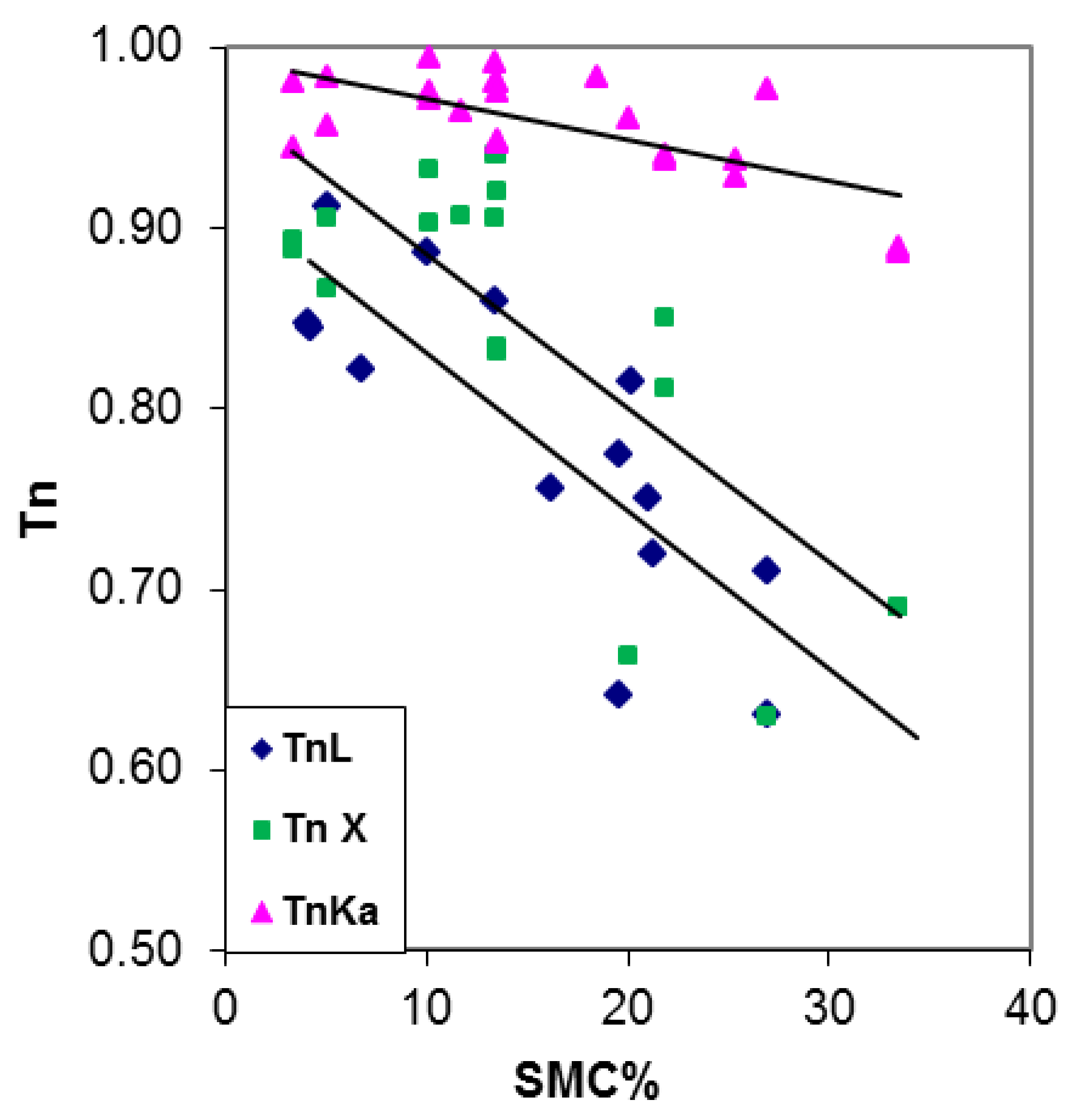
Microwave emission from non-vegetated soils is primarily sensitive to soil moisture due to the high contrast between the permittivity of dry matter and water. Besides, soil emission is influenced by surface roughness too, whose importance depends on the relative dimensions of the roughness parameters of the surface profile (i.e., Hstd, and Lc), and the observation wavelength, λ. Hence, the same surface can be “seen” as more or less rough depending on the observation frequency, as stated by the Rayleigh criterion. As predicted by theoretical models and confirmed by experiments, the effect of surface roughness is to increase emissivity and reduce the sensitivity to soil moisture. As an example, measurements carried out with ground based radiometer at L (λ = 21 cm), X (λ = 3.2 cm) and Ka (λ = 0.8 cm) bands on a sandy soil sample with a very smooth surface (Hstd < 1cm) are represented in Figure 2, which shows the normalized temperature (Tn), i.e., the brightness temperature (Tb) normalized to the thermometric surface temperature, as a function of soil moisture (SMC, in %) of the first soil layers. Due to the different penetration depths of the three frequency signals, data at L, X, and Ka bands have been correlated to the first 5.0, 2.5 and 1.0 cm layers, respectively. We can see that, for this very smooth surface, the sensitivity of Tn to SMC is almost the same at L and X bands (slope ≅ −0.0085), whereas it is significantly smaller at Ka band (−0.002), with rather low determination coefficient (R2 = 0.47) [21].
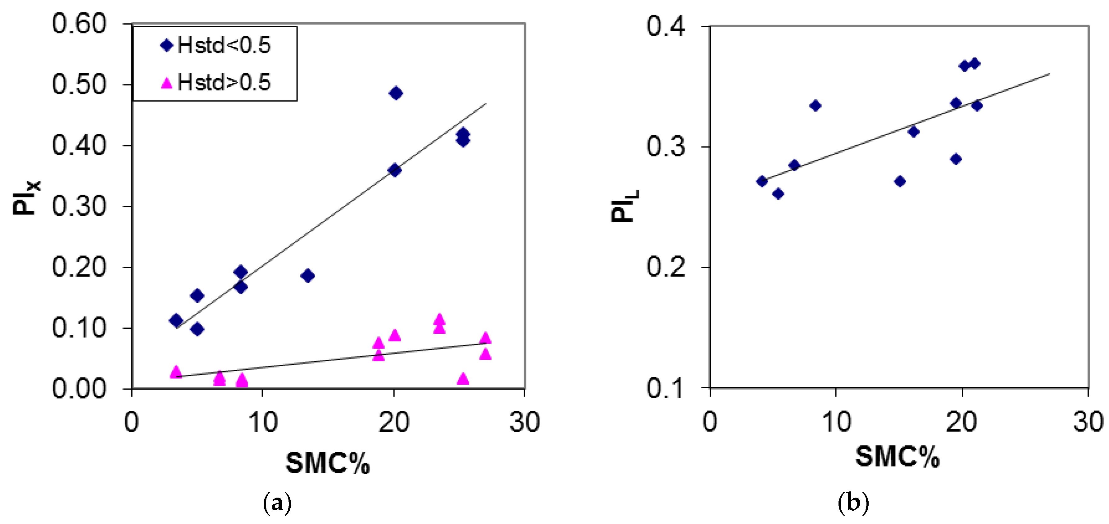
Also polarization is influenced by the moisture content. The behavior of the Polarization Index (the difference between the vertical, V, and horizontal, H, components of Tb normalized to their average value), PI = (Tbv − Tbh)/(1/2) (Tbv + Tbh) at L and X bands vs. SMC is represented in the diagrams of Figure 3a (X band) and Figure 3b (L band). PI at X band is significantly sensitive to SMC for smooth soils only (Hstd < 0.5cm), with R2 = 0.87 and slope 0.016, whereas, when Hstd is higher than 0.5 cm, the sensitivity to SMC becomes very low (R2 = 0.34 and slope 0.002). At L band the relationship between PI and SMC is similar for both types of surfaces (R2 = 0.46 and slope 0.004), confirming the scarce influence of surface roughness in this range of Hstd to the emission at this frequency.
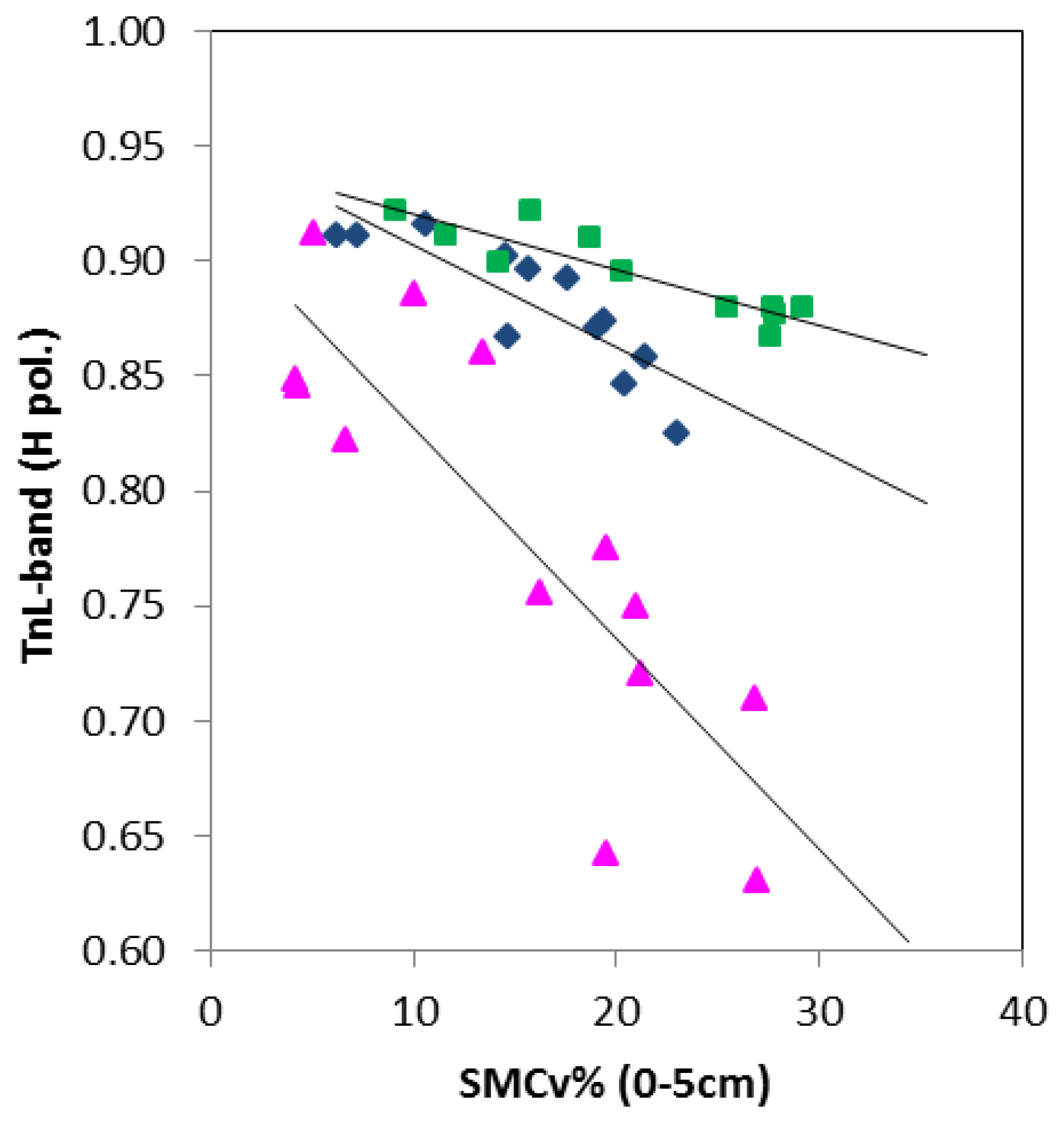
These results confirm that emission from natural terrains is influenced not only by SMC, but by the surface roughness too, which in general, increases the value of brightness temperature and reduces the sensitivity to SMC [22]. As an example, Figure 4 shows the Tn at L band as a function of SMC for three classes of roughness (Hstd < 0.4 cm, 0.7–1.2 cm, and 1.2–3.0 cm). We can note that even L band emission, in spite of the long wavelength, is influenced by surface roughness, especially when Hstd is higher than 1.2 cm. Although R2 remains almost the same for the 3 roughness classes (between 0.7 and 0.8), the slope significantly decreases (from −0.009 for smooth soils, to −0.0024 for the rougher surface), confirming that, as said, the same surface appears rougher at the smaller wavelengths.
Hence, a refinement of the measurements of SMC would require some knowledge of the surface roughness. A simple parametric model, which approximates fairly well the emissivity of a rough surface with Hsdt between 0 and 2.5 cm, in a frequency range between L and Ka bands, was developed by [23] by correcting the reflection coefficient with an exponential factor function of the square root of the wavelength. Other interesting approaches to account for the roughness effect were suggested by [24] and [25].
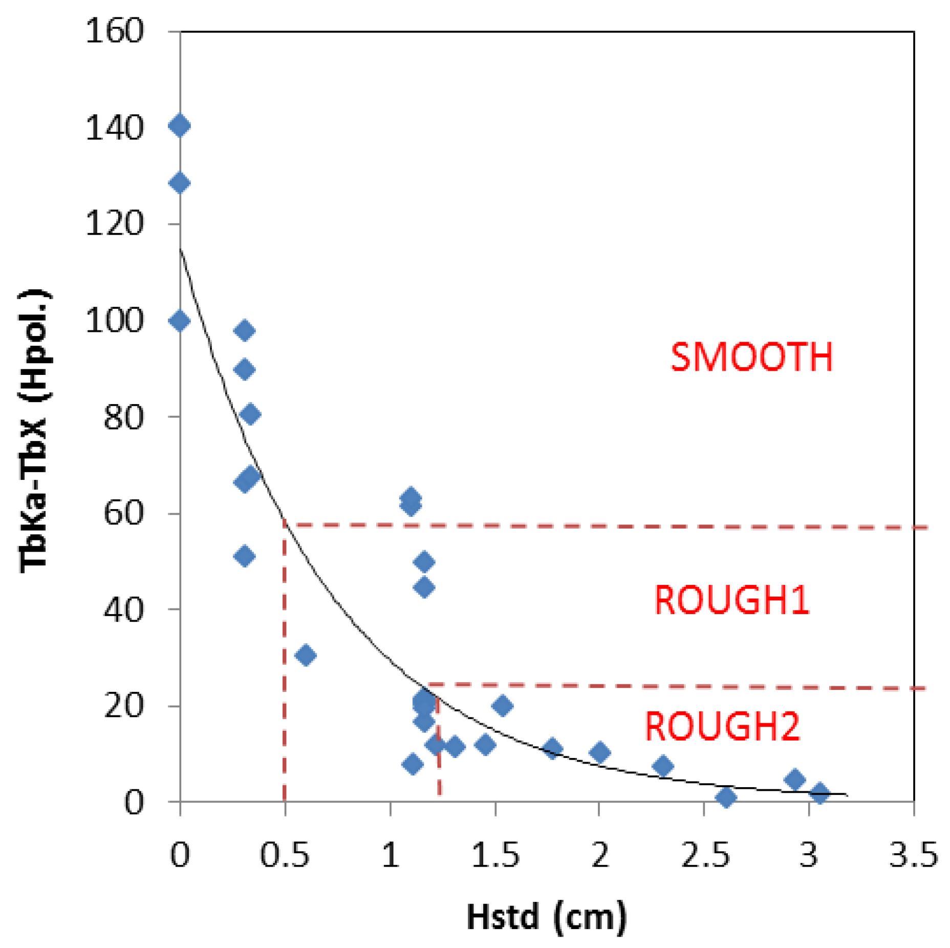
If dual or multi-frequency measurements are available, the effect of roughness on the measurement of SMC can be more easily evaluated. As an example, the index δTb (i.e., the difference TbKa − TbX), measured on surfaces with similar SMC but different roughness, shows a gradual decrease as the roughness increases, as it is shown in Figure 5.
In [21], this frequency index was related to the Hstd with an exponential function as: δTn = 114.7 exp(−1.36 Hstd), which approximates experimental data with R2 = 0.83. This approach allowed the identification of almost three ranges of roughness from Hstd < 1 cm to 2.5 cm and can provide a correction of the relationship between Tn at L band and SMC by separating measurements on surfaces characterized by different roughness.
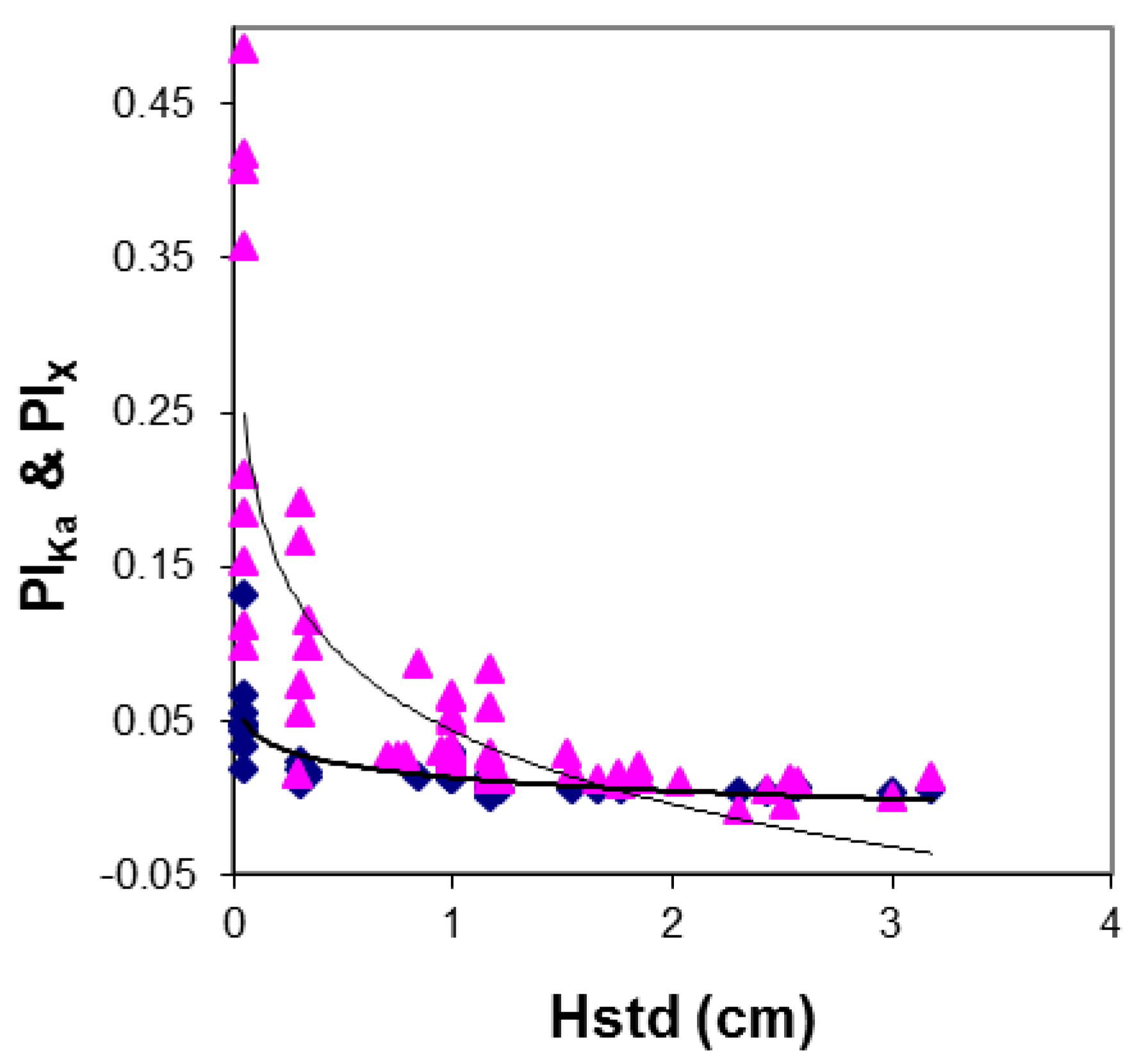
Another approach to evaluate the surface roughness is based on the measurements of the PI. Emission from a smooth flat surface at an incidence angle far from zenith is different for the two polarization V&H components as predicted by the Fresnel reflection coefficients. The presence of surface roughness tends to reduce or destroy this polarization difference, so that the measurement of PI can give a direct estimate of the surface Hstd. A direct relationship between PI, at both X and Ka bands, and Hstd is shown in Figure 6. We can see that in the range of Hstd between 0 and 3 cm, typical of most agricultural fields, PI at X band gradually decreases as Hstd increases (R2 = 0.65), although the experimental points are largely spread, whereas it quickly saturates at Ka band, as soon as Hstd becomes slightly > 0 cm (R2 = 0.55). From this diagram, it can be concluded that, the most appropriate frequency to perform this estimate of the surface Hstd in the range of roughness usually encountered in the agricultural fields is close to X band, which can allow the identification of 2–3 levels of roughness.
In summary, a combination of dual frequency/polarization data at Ka and X bands makes it possible to improve the accuracy of the SMC measurements based on L band data.
2.2. Vegetation
On vegetated surfaces, vegetation can be at the same time a disturbing factor for the estimate of soil moisture and a target for the measurements of vegetation biomass. In remote sensing, the latter is usually expressed by Plant Water Content (PWC, in Kg/m2), i.e., the total amount of water in plant elements per unit area. It should be noted that instead of our original notation PWC, most authors are now using the term Vegetation Water Content (VWC) (e.g., [10]).
Emission from vegetated surfaces is a combination of soil emission attenuated by the canopy with the emission from plant elements. In general, the contribution of vegetation increases with the observation frequency, f, and depends on the structure and dimensions of plant elements. The most commonly used for modeling microwave emission from soil covered by vegetation is the tau-omega (τ-ω) model, which is a simple formulation of RT transfer theory [26].
Also in this case, multi-frequency, dual polarization measurements can provide significantly more information than single channel observations. Indeed, depending on the type of plants and observation wavelength, Tb can increase or decrease as the biomass increases. This corresponds to different types of electromagnetic interactions. In general, absorption occurs for plant elements that are small with respect to observation wavelength, whereas scattering dominates in the opposite case [27].
On the other hand, the trend of the difference between the two linear polarization components (and then the PI), was found to be independent of the vegetation type and always decreasing as biomass increases [12]. Indeed, the polarized emission from an almost homogeneous and smooth soil is attenuated by the volumetric effect of any vegetation type [6]. Thus, significant information on vegetation biomass can be obtained by using PI, making it possible establishing an inversion approach to retrieve vegetation biomass independently of crop type.
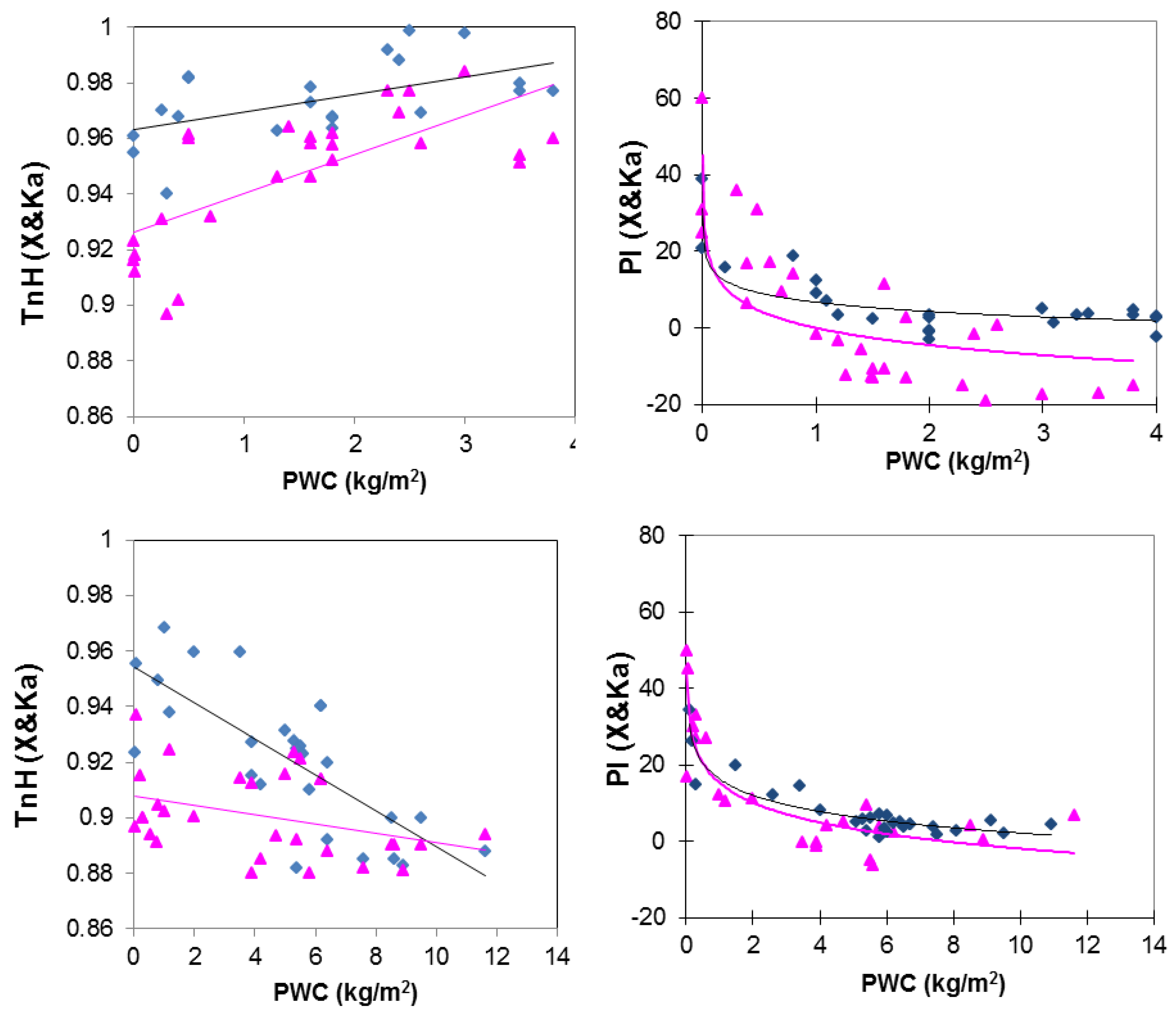
Figure 7 shows experimental values of Tn (in H pol.) (left) and PI at X and Ka bands (right) as a function of the PWC of two crop types: narrow-leaf crops (e.g., wheat and alfalfa), and broad-leaf crops (e.g., corn, sugar-beet and sunflower). In case of narrow-leaf crops, the mechanism of absorption is significant and Tb increases as PWC increases; whereas on broad-leaf crops scattering is dominant and Tb decreases with PWC. In all cases PI decreases as a function of increasing vegetation biomass, with a trend that is gradual at X band and rather steep at Ka band.
Table 1 shows the regression equations with the determination coefficients (R2) at the two frequencies for the two crop types.
These data obtained with ground-based sensors where positively compared with model simulations based on tau-omega (τ-ω) model in [28].
The results obtained from ground-based or airborne sensors have been confirmed by satellite investigations: a global map of vegetation cover based on the polarization difference at Ka band, obtained from Nimbus 7 data, was first shown in [7]. More recently, maps of PWC retrieved from PI at X band were obtained in the context of an algorithm based on an Artificial Neural Network (ANN) developed for generating simultaneous maps of SMC, PWC, and SD from the Advanced Multifrequency Scanning Radiometer (AMSR-E) [29,30].
2.3. Snow
The sensitivity of microwave emission to snow cover has been evident since the early experimental (e.g., [31,32]) and theoretical (e.g., [33]) studies.
Radiation emitted at lower frequencies of the microwave band (lower than about 6–10 GHz) by soil covered with a shallow layer of dry snow is mostly influenced by soil conditions below the snowpack. At higher frequencies and for thick snow layers, however, the role played by volume scattering increases, and microwave emission becomes sensitive to the presence of snow.
The most interesting parameter for hydrological applications is the snow water equivalent (SWE) equal to the product of snow depth (SD) by its density. As past research has demonstrated, the key-frequency channels for detecting the presence of snow and estimating SWE or SD are Ku and Ka bands. Measurements collected over several winter seasons on a relatively flat area located in Northeast Italy on Mount Cherz, by using ground-based radiometers at Ku and Ka bands, showed a decrease of Tb as the SWE increases up to about 260 mm at Ka band and 300mm at Ku. For SWE values beyond this value, Tb tends to increase again due to emission from the snowpack itself which masks the large scattering from the deep hoar (e.g., [34,35]). This trend, with some variability due to the snow characteristics, was observed in several other studies (e.g., [36,37,38]). Moreover, the range of SWE in which the minimum of Tb occurs depends on the penetration depths of radiation inside the snowpack.
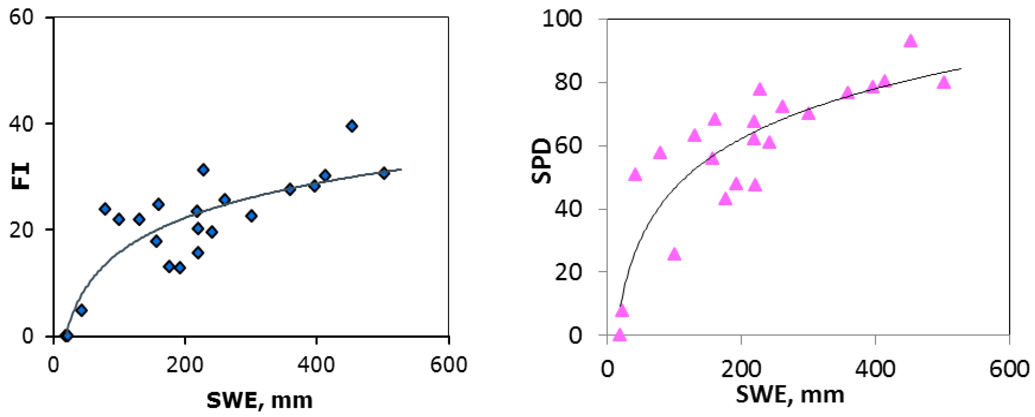
This reversal of brightness temperature at increasing SWE can cause ambiguity in the retrieval. In our measurements, after the inflection point, Tb shows a sharp increase at both frequencies and then tends to fluctuate with a relatively flat behavior. However, the difference between Tb at the two frequencies also tends to slightly increase after the threshold. Hence, we can speculate that, by using an appropriate combination of observation frequency and polarization the retrieval of SWE can be extended beyond the range 0–300 mm (e.g., [17,39,40]). For example, the Frequency Index (FI = ((TbKuV − TbKaV) + (TbKuH − TbKaH))/2) is sensitive to SWE and SD due to the fact that, in the case of dry snow, radiation at Ku band penetrates the snowpack with smaller attenuation and more deeply than the emission at the higher frequency (Ka band), which is more influenced by the scattering inside the snowpack [29]. The difference between the brightness at the two frequencies can therefore be linearly related, to some extent, to SD (and/or SWE). Other combinations of frequency channels and polarizations have also been tested to evaluate their sensitivity to SWE and, among these indices, the Spectral Polarization Difference defined as SPD = (TbKuV − TbKaV) + (TbKuV − TbKaH) was identified as the best correlated quantity to SD and SWE [38]. In summary, both FI and SPD present rather high correlation (in terms of R2) to SD and SWE, as demonstrated in [41], where the comparison of radiometric data with ground truth has shown the following logarithmic regressions: FI = 9.4 Ln(SWE) − 27.59 (R2 = 0.71); SPD = 22.76 Ln(SWE) − 58.32 (R2 = 0.76) in a range of SWE up to 500 mm. This result confirms that the use of dual-frequency/dual-polarization indices allows investigating snow properties, even beyond the inversion limit (Figure 8).
3. Model Simulations
3.1. Soil and Vegetation
Several models have been used for simulating brightness temperature and microwave indices from land surfaces. As per vegetation covered soils, the most used model is an approximate solution of the radiative transfer equation for a homogeneous soil overlaid by a medium at uniform temperature characterized either by small scattering (ks ≪ ka) or scattering “mainly forward”. In this approach, well-known as tau-omega (τ-ω) model [26], the parameters that characterize the absorbing and scattering properties of vegetation are the optical depth (τ) and the “albedo (ω). The radiation component due to vegetation is assumed to be unpolarized, whereas the radiation emitted from the smooth soil, and then by the whole canopy-soil system, is partially polarized.
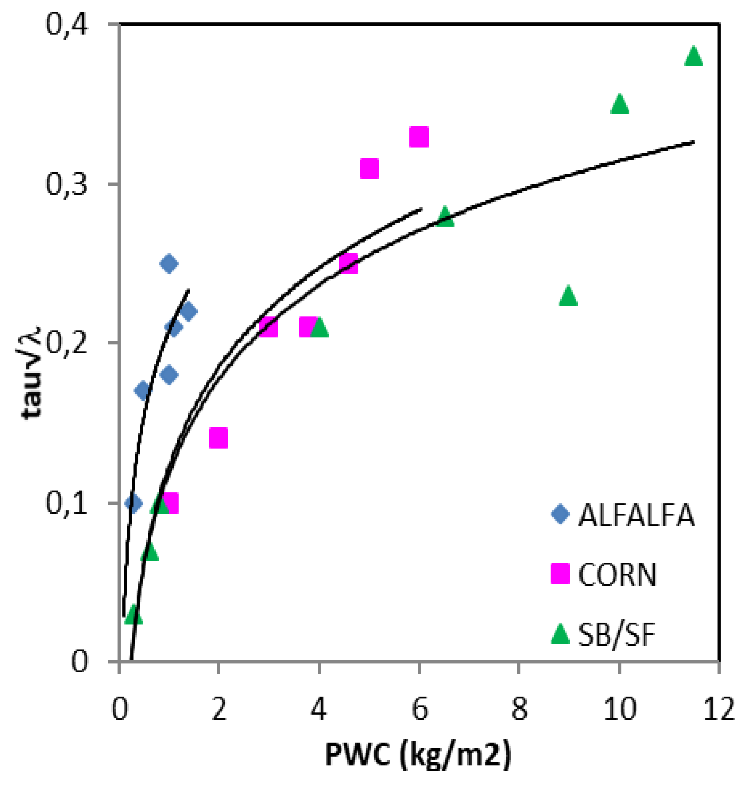
The key parameter of the (τ-ω) equation related to the vegetation biomass is vegetation optical depth (VOD or τ). This quantity increases as the canopy grows and, at L band, it has usually been related to the VWC/PWC with a linear relationship, for several crop types [42,43]. However, early studies at higher frequencies (X and Ka bands), had shown that experimental data can be fairly well approximated (R2 > 0.8) by the following logarithmic function [28,44], as it is shown in Figure 9:
where k is a constant depending on crop type, and λ is the wavelength of the emitted radiation. Equation (1) is represented in Figure 9 compared with experimental data for some crop types (alfalfa, corn, sugar beet and sunflower). The lines refer to the model obtained using two values of k (0.16 for alfalfa) and 0.4 for corn and sugar-beet) for better simulating the different crop types.
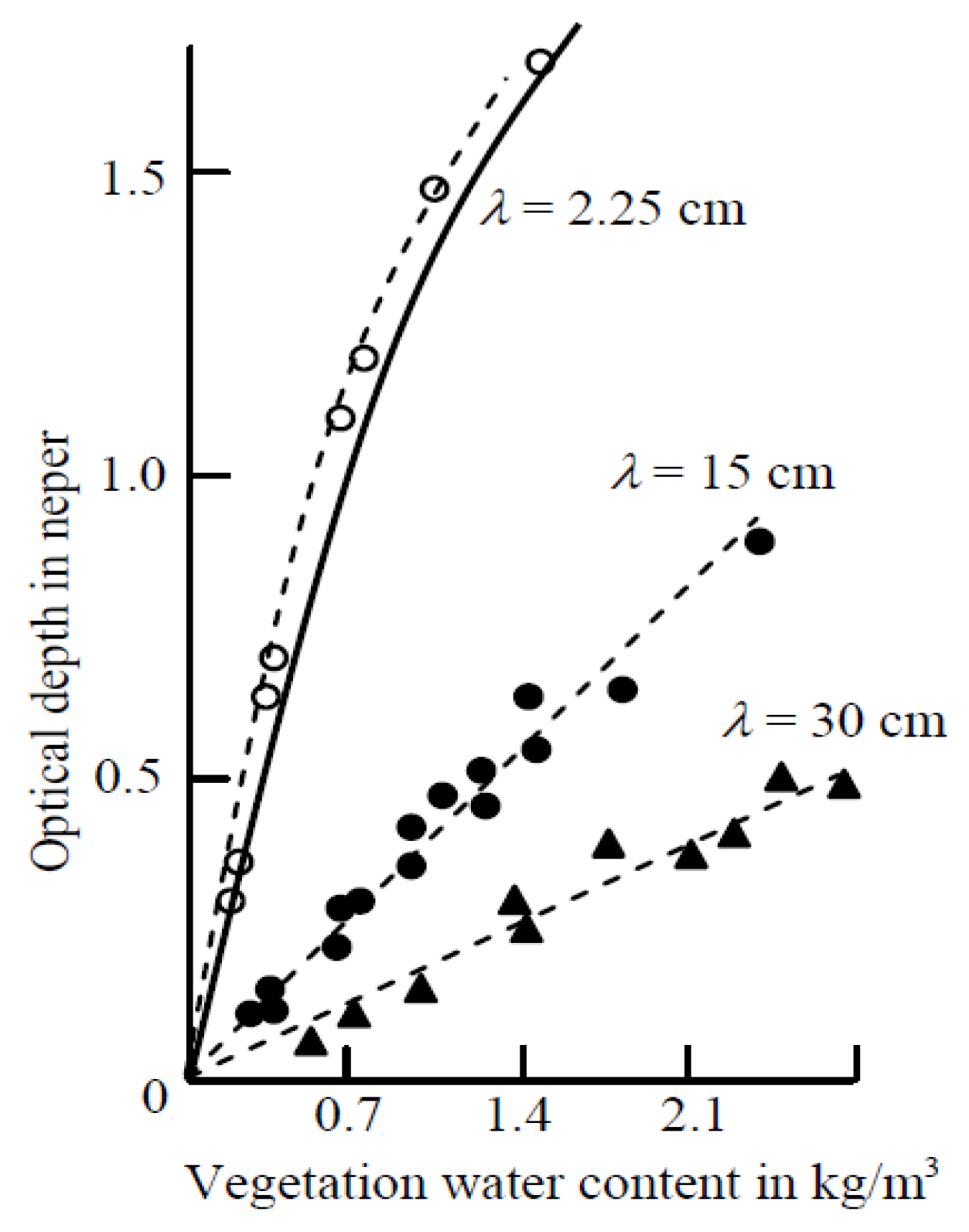
The conflict between the linear or logarithmic trend of τ versus PWC was clarified in [10] by expanding Equation (1) into power series (Equation (2)) and showing that this corresponds to the power expansion of the extinction coefficient, γ, of a collection of discrete scatterers computed with the radiative transfer theory. Hence, the linear relation between optical depth and PWC, frequently used at L band, agrees with the first term of this series and can be considered valid for low values of vegetation water content and long wavelengths:
where τ0 is the optical depth at low values of PWC.
In spite of the reduced range of the experimented PWC values (up to 2.5 Kg/m2), the progressive shift from linear to logarithmic relationship as the frequency increases is demonstrated in a study by [10,45] (Figure 10).
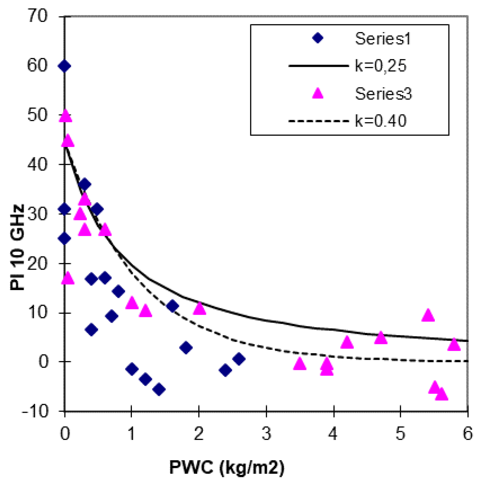
Figure 11 shows model simulations of PI (X band) as function of PWC compared with experimental data of two crop types: narrow-leaf (alfalfa and wheat) and broad-leaf (corn, sugar-beet and sunflower) crops. Here simulations are obtained by means of the τ-ω solution of the RT model, relating τ to PWC as in Equation (1) and using two values of k (0.16 and 0.40) for the two crop types. In the model, the scattering albedo, ω, the surface temperature, Ts, and the soil moisture, SMC, are kept constant and equal to 0.01, 290K, and 15%, respectively [6].
3.2. Snow
Microwave emission from for several types of terrestrial snow cover has been simulated using a multi-layer dense-medium radiative transfer model (DMRT) [46] implemented under the quasi crystalline approximation (ML-QCA). In particular, the model evaluated the sensitivity of the two FI and SPD indices on SWE comparing simulations to radiometric dual frequency/polarization measurements collected over three winter seasons between 2007 and 2011 in the Eastern Italian Alps [40].
In these simulations, inputs to the model were taken from ground data considering the changes in the snow structure (grain size, density, stickiness of snow particles, number and depth of layers) as SWE increased. The soil contribution was accounted for by using the Advanced Integral Equation Model (AIEM) [47] with a permittivity corresponding to frozen or moderately wet soil depending on the measured temperature.
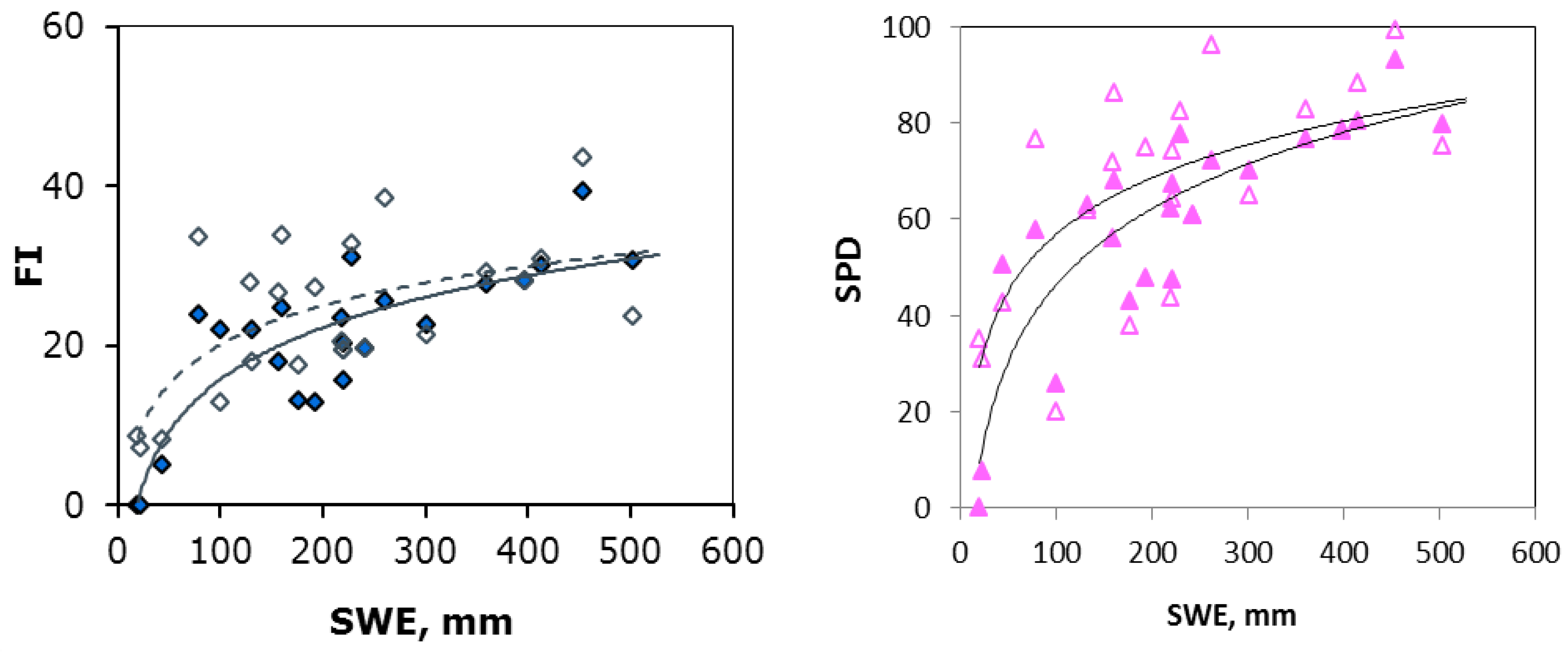
The simulations confirmed the sensitivity of these indices to SWE up to a value of 500 mm water equivalent (Figure 12). The regression equations obtained for both experimental and simulated data are the following:
FI = 9.4ln(SWE) − 27.6 (R2 = 0.71) (measured).
FI= 7.1ln(SWE) − 12.63 (R2 = 0.44) (modeled).
SPD = 22.76ln(SWE) − 58.32 (R2 = 0.76) (measured).
SPD = 16.89ln(SWE) −20.88 (R2 = 0.47) (modeled).
4. Observation from Satellite
Results obtained from satellite data (SSM/I, AMSR-E, AMSR2, SMAP) confirmed those obtained from ground-based and airborne sensors [48], by exploiting the potential of microwave indices in a global scale estimation of geophysical parameters, provided appropriate retrieval procedures are used. As an example, by including PI at X and Ku band in a SMC retrieval algorithm based on Artificial Neural Networks (ANN), a correlation coefficient R2 > 0.7 between retrieved and target SMC was obtained, while the correlation achievable on the same dataset by using only Tb at C band would have been lower, i.e., R ≃ 0.5 [49]. Other studies demonstrated the possibility of estimating SD in the Scandinavian peninsula, using PI and FI derived from AMSR-E, with RMSE = 9.13 cm and R2 ≃ 0.8 [29].
Another algorithm based on the joint use of PI at C, X and Ku band data derived from AMSR2 was able to produce global maps of vegetation biomass with a RMSE < 1 kg/m2 [30]. The validation of the latter algorithm, carried out on the entire Australian continent, demonstrated that the microwave data from AMSR2 can be legitimately used to produce vegetation maps on a global scale by separating several levels of biomass on low and medium dense vegetation (up to 8 Kg/m2), without any need of further information from other sensors and guaranteeing an all-weather monitoring.
5. Summary and Conclusions
Passive microwave remote sensing has been proved to be an important technique for monitoring land surfaces, and, in particular, three important parameters: soil moisture (SMC), vegetation biomass (PWC), and snow water equivalent (SWE). Unfortunately, all these parameters, together with some others (e.g., soil surface roughness/texture, vegetation/snow type), simultaneously affect microwave emission, so that the retrieval of the requested parameters is a typically ill-posed problem.
The complexity of the algorithms to be developed for retrieving spatial variations in land surface parameters depends on the auxiliary information available and on the direct models selected for the inversion procedures. Indeed, the more information (auxiliary or model derived) available, the more accurate but more complex algorithm can be developed. The analytical inversion of EM models is a complicated procedure, and generally, unfeasible without setting several boundary conditions. Different approaches have therefore been studied to provide information on all the factors that affect emission and reduce the effects of the undesired parameters, using ancillary or a-priori data. In this framework, the synergy between observations at different frequencies, polarizations, and incidence angles, significantly helps in improving the reliability of the inversion methods. A typical example is the polarization index (PI) at X band, which was confirmed to be the most suitable parameter for estimating vegetation biomass, and, furthermore, to be able to significantly increase the accuracy of the estimate of soil moisture based on L and C band data.
Concerning the retrieval of snow parameters, the Frequency Index (FI) and the Spectral Polarization Difference (SPD) demonstrated to be able to overcome the ambiguity introduced by the non-linear relationship between Tb and SWE, making it possible estimating SWE up to 500 mm.
Author Contributions
P.P. and S.P. conceived and performed the experiments, and analyzed the data through EM models; E.S. analyzed the satellite data and developed the retrieval algorithms.
Conflicts of Interest
The authors declare no conflicts of interest.
References
- Hollinger, J.; Lo, R.; Poe, G.; Savage, R.; Pierce, J. Special Sensor Microwave/Imager User’s Guide; Naval Res. Lab: Washington, DC, USA, 1987. [Google Scholar]
- Tucker, C.J. Red and Photographic Infrared Linear Combinations for Monitoring Vegetation. Remote Sens. Environ. 1979, 8, 127–150. [Google Scholar] [CrossRef]
- Huete, A.; Didan, K.; Miura, T.; Rodriguez, E.P.; Gao, X.; Ferreira, L.G. Overview of the radiometric and biophysical performance of the MODIS vegetation indices. Remote Sens. Environ. 2002, 83, 195–213. [Google Scholar] [CrossRef]
- Ulaby, F.T.; Moore, R.K.; Fung, A.K. Microwave Remote Sensing: Active and Passive; Addison-Wesley: Reading, MA, USA, 1982; Volume II. [Google Scholar]
- Ulaby, F.T.; Moore, R.K.; Fung, A.K. Microwave Remote Sensing: Active and Passive. Vol III; Artech House: Nordwood, MA, USA, 1986. [Google Scholar]
- Paloscia, S.; Pampaloni, P. Microwave Polarization Index for Monitoring Vegetation Growth. IEEE Trans. Geosci. Remote Sens. 1988, 26, 617–621. [Google Scholar] [CrossRef]
- Choudhury, B.J. Monitoring global land surface using Nimbus-7 37 GHz. Theory and examples. Int. J. Remote Sens. 1989, 10, 1579–1605. [Google Scholar] [CrossRef]
- Wang, J.; Choudhury, B. Remote sensing of soil moisture content over bare fields at 1.4 GHz frequency. J. Geophys. Res. 1981, 86, 5277–5282. [Google Scholar] [CrossRef]
- Kirdiashev, K.P.; Chukhlantsev, A.A.; Shutko, A.M. Microwave radiation of the Earth’s surface in the presence of vegetation cover. Radio Eng. Electron. Phys. Engl. Transl. 1979, 24, 256–264. [Google Scholar]
- Chukhlantsev, A.A. Microwave Radiometry of Vegetation Canopies; Springer: Dordrecht, The Netherlands, 2006. [Google Scholar]
- Neale, C.M.U.; Farland, M.J.M.; Chang, K. Land surface type classification using microwave brightness temperatures from the SMM/I. IEEE Trans. Geosci. Remote Sens. 1990, 28, 829–838. [Google Scholar] [CrossRef]
- Paloscia, S.; Pampaloni, P. Microwave Vegetation Indexes for detecting biomass and water conditions of agricultural crops. Remote Sens. Environ. 1992, 40, 15–26. [Google Scholar] [CrossRef]
- Shi, J.; Jackson, T.; Tao, J.; Du, J.; Bindlish, R.; Lu, L.; Chen, K.S. Microwave vegetation indices for short vegetation covers from satellite passive microwave sensor AMSR-E. Remote Sens. Environ. 2008, 112, 4285–4300. [Google Scholar] [CrossRef]
- Hallikainen, M.T.; Jolma, P.A. Comparison of algorithms for retrieval of snow water equivalent from Nimbus-7 SMMR data in Finland. IEEE Trans. Geosci. Remote Sens. 1992, 30, 124–131. [Google Scholar] [CrossRef]
- Hallikainen, M.T. Retrieval of snow water equivalent from Nimbus-7 SMMR data: Effect of land-cover categories and weather conditions. IEEE J. Ocean. Eng. 1984, 9, 372–376. [Google Scholar] [CrossRef]
- Kelly, R.; Chang, A.T.C. Development of a passive microwave global snow depth retrieval algorithm for Special Sensor Microwave Imager (SSM/I) and Advanced Microwave Scanning Radiometer-EOS (AMSR-E) data. Radio Sci. 2003, 38, 8076. [Google Scholar] [CrossRef]
- Chang, T.C.; Foster, J.L.; Hall, D.K.; Rango, A.; Hartline, B.K. Snow water equivalent estimation by microwave radiometry. Cold Reg. Sci. Technol. 1982, 5, 259–267. [Google Scholar] [CrossRef]
- Foster, J.L.; Chang, A.T.C.; Hall, D.K. Comparison of snow mass estimates from a prototype passive microwave snow algorithm, a revised algorithm and a snow depth climatology. Remote Sens. Environ. 1997, 62, 132–142. [Google Scholar] [CrossRef]
- Aschbacher, J. Microwave Signatures from Land surface Radiometry. In Proceedings of the 10th Annual International Symposium on Geoscience and Remote Sensing IGARSS 1990, College Park, MD, USA, 20–24 May 1990; pp. 1149–1152. [Google Scholar]
- Tsutsui, H.; Koike, T. Development of Snow Retrieval Algorithm Using AMSR-E for the BJ Ground-Based Station on Seasonally Frozen Ground at Low Altitude on the Tibetan Plateau. J. Meteorol. Soc. Jpn. 2012, 90, 99–112. [Google Scholar] [CrossRef]
- Paloscia, S.; Pampaloni, P.; Chiarantini, L.; Coppo, P.; Gagliani, S.; Luzi, G. Multifrequency passive microwave remote sensing of soil moisture and roughness. Int. J. Remote Sens. 1993, 14, 467–483. [Google Scholar] [CrossRef]
- Choudhury, B.J.; Schmugge, T.J.; Chang, A.; Newton, R.W. Effect of Surface Roughness on the Microwave Emission from Soils. J. Geophys. Res. 1979, 84, 5699–5706. [Google Scholar] [CrossRef]
- Coppo, P.; Luzi, G.; Paloscia, S.; Pampaloni, P. Effect of soil roughness on microwave emission: Comparison between experimental data and model. In Proceedings of the Remote Sensing: Global Monitoring for Earth Management, IGARSS ’91, Espoo, Finland, 3–6 June 1991; pp. 1167–1170. [Google Scholar] [CrossRef]
- Wegmuller, U.; Maetzler, C. Rough bare soil reflectivity model. IEEE Trans. Geosci. Remote Sens. 1999, 37, 1391–1395. [Google Scholar] [CrossRef]
- Chen, M.; Weng, F. Modeling Land Surface Roughness Effect on Soil Microwave Emission in Community Surface Emissivity Model. IEEE Trans. Geosci. Remote Sens. 2016, 54, 1716–1726. [Google Scholar] [CrossRef]
- Mo, T.; Choudhury, B.J.; Schmugge, T.J.; Wang, J.R.; Jackson, T.J. A model for microwave emission from vegetation-covered fields. J. Geophys. Res. 1982, 87, 11229–11237. [Google Scholar] [CrossRef]
- Ferrazzoli, P.; Paloscia, S.; Pampaloni, P.; Schiavon, G.; Solimini, D.; Coppo, P. Sensitivity of Microwave Measurements to Vegetation Biomass and Soil Moisture Content: A Case Study. IEEE Trans. Geosci. Remote Sens. 1992, 30, 750–756. [Google Scholar] [CrossRef]
- Paloscia, S. Microwave emission from vegetation. In Passive Microwave Remote Sensing of Land-Atmosphere Interactions; Choudhury, B., Njoku, E., Kerr, Y., Pampaloni, P., Eds.; VSP Press: Zeist, The Netherlands, 1995; pp. 358–374. [Google Scholar]
- Santi, E.; Pettinato, S.; Paloscia, S.; Pampaloni, P.; Macelloni, G.; Brogioni, M. An algorithm for generating soil moisture and snow depth maps from microwave spaceborne radiometers: HydroAlgo. Hydrol. Earth Syst. Sci. 2012, 16, 3659–3676. [Google Scholar] [CrossRef] [Green Version]
- Santi, E.; Paloscia, S.; Pampaloni, P.; Pettinato, S.; Tomoyuki, N.; Seki, M.; Sekiya, K.; Maeda, T. Vegetation Water Content Retrieval by Means of Multifrequency Microwave Acquisitions from AMSR2. IEEE J. Sel. Top. Appl. Earth Obs. Remote Sens. 2017, 10, 3861–3873. [Google Scholar] [CrossRef]
- Kunzi, K.F.; Fisher, A.D.; Staelin, D.H.; Waters, J.W. Snow and ice surfaces measured by the Nimbus 5 microwave spectrometer. J. Geophys Res. 1976, 81, 4965–4980. [Google Scholar] [CrossRef]
- Hofer, R.; Mätzler, C. Investigation of snow parameters by radiometry in the 3- to 60-mm wavelength region. J. Geophys. Res. 1980, 85, 453–460. [Google Scholar] [CrossRef]
- Jin, Y.Q.; Kong, J.A. Strong fluctuation theory of electromagnetic wave scattering by a layer of random discrete scatterers. J. Appl. Phys. 1984, 55, 1364–1369. [Google Scholar] [CrossRef]
- Dong, J.; Walker, J.P.; Houser, P.R. Factors affecting remotely sensed snow water equivalent uncertainty. Remote Sens. Environ. 2005, 97, 68–82. [Google Scholar] [CrossRef]
- Markus, T.; Powell, D.C.; Wang, J.R. Sensitivity of passive microwave snow depth retrievals to weather effects and snow evolution. IEEE Trans. Geosci. Remote Sens. 2006, 44, 68–77. [Google Scholar] [CrossRef]
- Langlois, A.; Royer, A.; Derksen, C.; Montpetit, B.; Dupont, F.; Goïta, K. Coupling the snow thermodynamic model SNOWPACK with the microwave emission model of layered snowpacks for subarctic and arctic snow water equivalent retrievals. Water Resour. Res. 2012, 48, 1–14. [Google Scholar] [CrossRef]
- Schanda, E.; Matzler, C.; Kunzi, K. Microwave remote sensing of snow cover. Int. J. Remote Sens. 1982, 4, 149–158. [Google Scholar] [CrossRef]
- Takala, M.; Luojus, K.; Pulliainen, J.; Derksen, C.; Lemmetyinen, J.; Kärnä, J.P.; Koskinen, J.; Bojkov, B. Estimating northern hemisphere snow water equivalent for climate research through assimilation of space-borne radiometer data and ground-based measurements. Remote Sens. Environ. 2011, 115, 3517–3529. [Google Scholar] [CrossRef]
- Tait, A.B. Estimation of Snow Water Equivalent Using Passive Microwave Radiation Data. Remote Sens. Environ. 1988, 64, 286–291. [Google Scholar] [CrossRef]
- Santi, E.; Paloscia, S.; Pampaloni, P.; Pettinato, S.; Brogioni, M.; Xiong, C.; Crepaz, A. Analysis of Microwave Emission and Related Indices Over Snow using Experimental Data and a Multilayer Electromagnetic Model. IEEE Trans. Geosci. Remote Sens. 2017, 99, 1–14. [Google Scholar] [CrossRef]
- Rott, H.; Aschbacher, J. On the use of satellite microwave radiometers for large-scale hydrology. In Proceedings of the IAHS 3rd International Assembly on Remote Sensing and Large-Scale Global Processes, Baltimore, MD, USA, 10–19 May 1989. [Google Scholar]
- Chukhlantsev, A.A. Microwave Emission from Vegetation Canopies. Ph.D. Thesis, The Moscow Institute of Physics and Technology (State University), Moscow, Russia, 1981. (In Russian). [Google Scholar]
- Jackson, T.J.; Schmugge, T.J.; Wang, J.R. Passive microwave sensing of soil moisture under vegetation canopies. Water Resour. Res. 1982, 18, 1137–1142. [Google Scholar] [CrossRef]
- Pampaloni, P.; Paloscia, S. Microwave emission and plant water content: A comparison between field measurement and theory. IEEE Trans. Geosci. Remote Sens. 1986, 24, 900–905. [Google Scholar] [CrossRef]
- Chukhlantsev, A.A.; Golovachev, S.P.; Shutko, A.M. Experimental study of vegetable canopy microwave emission. Adv. Space Res. 1989, 9, 317–321. [Google Scholar] [CrossRef]
- Tsang, L.; Pan, J.; Liang, D.; Li, Z.X.; Cline, D.; Tan, Y.H. Modeling active microwave remote sensing of snow using dense media radiative transfer (DMRT) theory with multiple scattering effects. IEEE Trans. Geosci. Remote Sens. 2007, 45, 990–1004. [Google Scholar] [CrossRef]
- Wu, T.D.; Chen, K.S. A Reappraisal of the Validity of the IEM Model for Backscattering from Rough Surfaces. IEEE Trans. Geosci. Remote Sens. 2004, 42, 743–753. [Google Scholar]
- Macelloni, G.; Paloscia, S.; Pampaloni, P.; Santi, E. Global scale monitoring of soil and vegetation using active and passive sensors. Int. J. Remote Sens. 2003, 24, 2409–2425. [Google Scholar] [CrossRef]
- Santi, E.; Paloscia, S.; Pettinato, S.; Brocca, L.; Ciabatta, L. Robust Assessment of an Operational Algorithm for the Retrieval of Soil Moisture from AMSR-E Data in Central Italy. IEEE J. Sel. Top. Appl. Earth Obs. Remote Sens. 2016, 9, 2478–2492. [Google Scholar] [CrossRef]
Figure 1.
Installations of IROE microwave radiometers on several platforms: in a shelter on snow, on hydraulic booms on forest and agricultural fields, and on helicopter and ultra-light aircraft.
Figure 1.
Installations of IROE microwave radiometers on several platforms: in a shelter on snow, on hydraulic booms on forest and agricultural fields, and on helicopter and ultra-light aircraft.

Figure 2.
The normalized Temperature (Tn, i.e., the ratio between brightness temperature, and thermal surface temperature, at Ka, X, and L as a function of SMC% of a bare smooth sandy soil.
Figure 2.
The normalized Temperature (Tn, i.e., the ratio between brightness temperature, and thermal surface temperature, at Ka, X, and L as a function of SMC% of a bare smooth sandy soil.

Figure 3.
(a) PI at X band (PIX) vs. SMC for 2 surface types; (b) PI at L band (PIL) vs. SMC.

Figure 4.
Tn (L band, Hpol, Θ = 10°–20°) as a function of volumetric SMC (0–5 cm) for three different ranges of surface roughness Hstd (∙ ≤ 0.4 cm, ◊ = 0.7–1.2 cm, Δ = 1.2–3.0 cm).
Figure 4.
Tn (L band, Hpol, Θ = 10°–20°) as a function of volumetric SMC (0–5 cm) for three different ranges of surface roughness Hstd (∙ ≤ 0.4 cm, ◊ = 0.7–1.2 cm, Δ = 1.2–3.0 cm).

Figure 5.
δTb = TbKa − TbX at θ = 40° and H pol. as a function of Hstd (After [21]).
Figure 5.
δTb = TbKa − TbX at θ = 40° and H pol. as a function of Hstd (After [21]).

Figure 6.
PI, at X (triangles) and Ka (rhombs) bands, vs. Hstd.

Figure 7.
left: Normalized Temperature (Tn, in H pol.) at X (triangles) and Ka (rhombs) bands as a function of PWC, and right: PI at X and Ka bands as a function of PWC, for two different crop types: narrow-leaf crops (e.g., wheat and alfalfa) (top), and broad-leaf crops (e.g., corn, sugar beet and sunflower) (bottom).

Figure 8.
FI and SPD as a function of SWE (mm). The regression lines are: FI = 9.4 Ln(SWE) − 27.6 (R 2 = 0.71); SPD = 22.76 Ln(SWE) − 58.3 (R2 = 0.76).
Figure 8.
FI and SPD as a function of SWE (mm). The regression lines are: FI = 9.4 Ln(SWE) − 27.6 (R 2 = 0.71); SPD = 22.76 Ln(SWE) − 58.3 (R2 = 0.76).

Figure 9.
Relationship between τ√λ and PWC for some crop types: alfalfa, corn, sugar-beet (SB) and sunflower (SF).
Figure 9.
Relationship between τ√λ and PWC for some crop types: alfalfa, corn, sugar-beet (SB) and sunflower (SF).

Figure 10.
Dependence of optical depth on PWC. Solid curve is calculated by the model of Equation (1) (After [10]).
Figure 10.
Dependence of optical depth on PWC. Solid curve is calculated by the model of Equation (1) (After [10]).

Figure 11.
Simulations of PI (at X band) as a function of PWC compared with experimental data of two crop types: narrow-leaf (alfalfa and sugar beet, rhombs) and broad-leaf (corn and sunflower, triangles).
Figure 11.
Simulations of PI (at X band) as a function of PWC compared with experimental data of two crop types: narrow-leaf (alfalfa and sugar beet, rhombs) and broad-leaf (corn and sunflower, triangles).

Figure 12.
FI and SPD vs. SWE. The empty dots represent the model simulations carried out with the DMRT model, and the full dots the experimental data. Lines represent the regression equations for both simulated (dashed lines) and experimental (continuous lines) data.
Figure 12.
FI and SPD vs. SWE. The empty dots represent the model simulations carried out with the DMRT model, and the full dots the experimental data. Lines represent the regression equations for both simulated (dashed lines) and experimental (continuous lines) data.


Table 1.
Regression equations and R2 between Tn and PWC, and PI and PWC, at X and Ka bands.
| Crop Type | Tn Regression Lines | R2 | PI Regression Lines | R2 |
|---|---|---|---|---|
| Narrow-leaf | TnX = 0.014PWC + 0.93 | 0.5 | PIX = −0.5ln(PWC) + 0.077 | 0.6 |
| Narrow-leaf | TnKa = 0.0063PWC + 0.96 | 0.3 | PIKa = −3.52ln(PWC) + 6.77 | 0.74 |
| Broad-leaf | TnX = −0.002PWC + 0.91 | 0.13 | PIX = −7.51ln(PWC) + 15.35 | 0.79 |
| Broad-leaf | TnKa = −0.0065PWC + 0.95 | 0.57 | PIKa = −6.17ln(PWC) + 16.34 | 0.85 |
© 2018 by the authors. Licensee MDPI, Basel, Switzerland. This article is an open access article distributed under the terms and conditions of the Creative Commons Attribution (CC BY) license (http://creativecommons.org/licenses/by/4.0/).
Share and Cite
MDPI and ACS Style
Paloscia, S.; Pampaloni, P.; Santi, E. Radiometric Microwave Indices for Remote Sensing of Land Surfaces. Remote Sens. 2018, 10, 1859. https://0-doi-org.brum.beds.ac.uk/10.3390/rs10121859
AMA Style
Paloscia S, Pampaloni P, Santi E. Radiometric Microwave Indices for Remote Sensing of Land Surfaces. Remote Sensing. 2018; 10(12):1859. https://0-doi-org.brum.beds.ac.uk/10.3390/rs10121859
Chicago/Turabian StylePaloscia, Simonetta, Paolo Pampaloni, and Emanuele Santi. 2018. "Radiometric Microwave Indices for Remote Sensing of Land Surfaces" Remote Sensing 10, no. 12: 1859. https://0-doi-org.brum.beds.ac.uk/10.3390/rs10121859
Note that from the first issue of 2016, this journal uses article numbers instead of page numbers. See further details here.