Spectral Mixture Analysis as a Unified Framework for the Remote Sensing of Evapotranspiration


Lamont-Doherty Earth Observatory, Columbia University, Palisades, NY 10964, USA
*
Author to whom correspondence should be addressed.
Remote Sens. 2018, 10(12), 1961; https://0-doi-org.brum.beds.ac.uk/10.3390/rs10121961
Submission received: 24 October 2018
/
Revised: 1 December 2018
/
Accepted: 1 December 2018
/
Published: 5 December 2018
(This article belongs to the Special Issue Advances in the Remote Sensing of Terrestrial Evaporation)
Abstract
:This study illustrates a unified, physically-based framework for mapping landscape parameters of evapotranspiration (ET) using spectral mixture analysis (SMA). The framework integrates two widely used approaches by relating radiometric surface temperature to subpixel fractions of substrate (S), vegetation (V), and dark (D) spectral endmembers (EMs). Spatial and temporal variations in these spectral endmember fractions reflect process-driven variations in soil moisture, vegetation phenology, and illumination. Using all available Landsat 8 scenes from the peak growing season in the agriculturally diverse Sacramento Valley of northern California, we characterize the spatiotemporal relationships between each of the S, V, D land cover fractions and apparent brightness temperature (T) using bivariate distributions in the ET parameter spaces. The dark fraction scales inversely with shortwave broadband albedo (ρ < −0.98), and show a multilinear relationship to T. Substrate fraction estimates show a consistent (ρ ≈ 0.7 to 0.9) linear relationship to T. The vegetation fraction showed the expected triangular relationship to T. However, the bivariate distribution of V and T shows more distinct clustering than the distributions of Normalized Difference Vegetation Index (NDVI)-based proxies and T. Following the Triangle Method, the V fraction is used with T to compute the spatial maps of the ET fraction (EF; the ratio of the actual total ET to the net radiation) and moisture availability (Mo; the ratio of the actual soil surface evaporation to potential ET at the soil surface). EF and Mo estimates derived from the V fraction distinguish among rice growth stages, and between rice and non-rice agriculture, more clearly than those derived from transformed NDVI proxies. Met station-based reference ET & soil temperatures also track vegetation fraction-based estimates of EF & Mo more closely than do NDVI-based estimates of EF & Mo. The proposed approach using S, V, D land cover fractions in conjunction with T (SVD+T) provides a physically-based conceptual framework that unifies two widely-used approaches by simultaneously mapping the effects of albedo and vegetation abundance on the surface temperature field. The additional information provided by the third (Substrate) fraction suggests a potential avenue for ET model improvement by providing an explicit observational constraint on the exposed soil fraction and its moisture-modulated brightness. The structures of the T, EF & Mo vs SVD feature spaces are complementary and that can be interpreted in the context of physical variables that scale linearly and that can be represented directly in process models. Using the structure of the feature spaces to represent the spatiotemporal trajectory of crop phenology is possible in agricultural settings, because variations in the timing of planting and irrigation result in continuous trajectories in the physical parameter spaces that are represented by the feature spaces. The linear scaling properties of the SMA fraction estimates from meter to kilometer scales also facilitate the vicarious validation of ET estimates using multiple resolutions of imagery.
1. Introduction
Water is critical to life on Earth: metabolic pathways rely on the chemistry of aqueous solutions, plant physiology requires cooling through stomatal water loss, and landscape-scale patterns in ecological communities often develop around the availability of near-surface water (or lack thereof). The movement of water between components of the Earth system therefore connects the biosphere with the lithosphere and the atmosphere. Evapotranspiration (ET; the sum of evaporation and transpiration) is a central mechanism in this exchange, describing the directional transfer of water from the Earth’s surface to its atmosphere. In addition to its importance for global biogeochemical cycles, ET also plays a major role in Earth’s surface energy balance (SEB). The thermodynamic implications of ET in the SEB result in its fundamental importance in the climate system, where clear global teleconnections are observed between ET and phenomena such as the El Niño–Southern Oscillation [1], in addition to direct relationships between soil moisture and temperature [2]. The sheer variety of biogeophysical systems that are impacted by ET demonstrate the importance of accurate global distributions of the components of ET [3] and characterization of multidecadal trends [4] for our understanding of, and ability to predict changes in, fundamental aspects of the Earth system.
In addition to its importance for understanding fundamental Earth system processes, ET also has clear practical applications. ET has long been recognized as a practical indicator of plant water stress [5,6,7]. In agricultural settings, ET monitoring has been used for water resource regulation and planning in water-limited regions such as the western United States [8] as well as to improve estimates of irrigation need [9,10]. In natural environments, ET has been used for global biodiversity assessments [11,12] as well as to assess regional water consumption by invasive species [13]. For recent reviews of the potential applications of ET monitoring, as well as outstanding unresolved questions, see [14].
Despite its centrality to such a wide range of fundamental Earth systems, accurate and consistent estimation of ET remains a challenge. For instance, a recent analysis found that over 50 models currently exist to compute potential ET, and that model choice can impact flux estimates by over 25% [11]. Uncertainty in ET estimation has substantial implications for our ability to manage agriculture and to monitor wildlands, as well as for our understanding of deeper questions about the Earth system, such as the amplitude of global water and energy fluxes. This uncertainty is, at least in part, a result of differences in the data streams, underlying assumptions, and conceptual approaches that are used by each model. The more that these disparities can be integrated into a single framework, the more that it will be possible to reduce the overall uncertainty in ET estimation.
Algorithms that estimate ET parameters on landscape scales generally rely on observations from optical and thermal remote sensing. For ET studies, remote sensing observations are most commonly used to provide direct estimates of fractional vegetation cover (V), surface temperature (T), and albedo (α). The relationships among these three quantities can be understood in the context of their bivariate distributions. The distribution of V vs T gives information about plant-based evapotranspirative cooling and is fundamental to the physical basis of many popular ET models (e.g., [15,16,17,18]). Leaf area index (LAI) is an additional parameter that has been shown to have a significant impact on ET partitioning [19], and it is often used as an input in ET models. However, remote sensing is generally used to estimate LAI using a direct empirical relationship with V. Because of this intrinsic dependence between the remote sensing estimates of LAI and V, the LAI vs T and V vs T relationships contain fundamentally similar information. The distribution of α vs T has also been long recognized [20], and provides information about soil moisture ([21,22]) and roughness [23]. α vs T has been incorporated into a popular ET model by [24]. Recent work by [25] has developed a model based on fusion of both the V vs T and α vs T relationships, with encouraging results.
For the vast majority of current ET estimation algorithms and associated Surface–Vegetation–Atmosphere Transfer (SVAT) models, vegetation abundance is computed with a spectral index. The specific index used varies from model to model, but all spectral indices use only part of the information present in multispectral imagery. Many models (e.g., [26,27]) rely directly upon the Normalized Difference Vegetation Index (NDVI). NDVI has a number of known flaws, including scaling nonlinearities ([28,29,30]), sensitivity to both soil background and atmospheric effects ([31,32]), and saturation effects over a wide range of vegetation fractions [32]. In an attempt to mitigate these problems, NDVI is often normalized using linear (e.g., [33]) or quadratic (e.g., [34,35,36]) transformations. Each spectral index, transformed or untransformed, gives different estimates of vegetation abundance, which then result in differences in the estimated ET. If these metrics could be improved and standardized, ET models could be made more accurate, and cross-model standardization could be more effective. One recent study [37] has recognized the impact of subpixel heterogeneity on ET model accuracy and used a spectral mixture model to estimate subpixel fractions of different agricultural crops with different ET characteristics. These crop fractions were used as inputs to the SEBAL and SEBS models, resulting in improved accuracies of between 7% and 18% for different crop types.
Spectral Mixture Analysis (SMA; [38,39,40]) is a physically-based method that uses the full reflectance spectrum, rather than a subset of bands, to estimate V simultaneously with fractions of other spectral endmembers within each pixel’s field of view. SMA can explicitly account for illumination effects, as well the reflectance of the soil and non-photosynthetic vegetation (NPV) background, substantially improving estimates at low vegetation abundance [31]. Because SMA relies on the area-weighted linear mixing of radiance from materials within the pixel, V estimates are relatively insensitive to sensor spatial resolution, and they have been shown to scale linearly from 2 m to 30 m [30,32], as well as from meter-scale field measurements [28]. This simple linear scaling could be a key advantage for ET studies, given the widely recognized scaling nonlinearities of many ET estimates (e.g., [41,42,43,44,45,46]). SMA fraction estimates are sensitive to the spectra of the endmember (EM) materials, but previous work has characterized the global multispectral mixing space and proposed standardized generic EMs, which well-describe the majority of the Earth’s land environments, and are calibrated across sensors ([32,47,48]).
In addition to providing enhanced estimates of V, SMA simultaneously provides accurate estimates of two additional physically meaningful quantities: (1) the subpixel areal abundances of soil, rock, and NPV substrates (S), and (2) dark features (D) such as shadow, water, and low-albedo surfaces. These estimates are made at subpixel resolution and with trivial computational cost. Dark fraction estimates represent the effects of albedo (α), illumination geometry (flux density), atmospheric opacity, and soil moisture content, thereby modulating the overall amplitude of the reflectance signal. Substrate fraction estimates provide information about the compositional properties of the soil, and NPV substrate background at each pixel. To our knowledge, the simultaneous estimation of vegetation fraction, soil+NPV background, and albedo provided by standardized SMA has not yet been incorporated into ET estimation approaches. This could represent a missed opportunity. When compared against coincident T measurements, SVD fractions can provide a unifying framework which incorporates two major existing approaches to ET estimation (V vs T and α vs T), and also includes a novel, potentially useful supplement (S vs T). By estimating S, V, and D fractions simultaneously, SMA automatically provides information on their respective contributions to the aggregate reflectance spectrum of each pixel. Therefore, multitemporal SVD fractions provide a self-consistent measure of the time-varying tradeoff between illuminated vegetation and soil fractions and moisture-modulated soil albedo—two of the primary factors determining the combined evaporative and transpirative processes that control the surface temperature field.
The primary purpose of this analysis is to explore the SVD model as a conceptual framework for ET estimation. While the V vs T relationship has been long recognized in ET studies [29,49], to our knowledge it has been only investigated using NDVI and its transformations, not by V as estimated by standardized SMA. Similarly, the α vs T relationship has already been explored, but only by estimating α through forward modeling. The connection between the α vs T and D vs T relationships has not yet been documented. In addition, to our knowledge, the relationships between S, V, D, and the ET Fraction (EF) and Moisture Availability (Mo) estimates have not yet been characterized. Finally, we evaluate the EF and Mo estimates using weather station data, and discuss the implications of this approach for improving the accuracy and consistency of ET estimates, informing flux partitioning, and providing an optimized, unifying approach to extract maximum value from coincident multispectral and multiresolution optical and thermal imagery.
1.1. ET Model Overview
1.1.1. Models Relying on V vs T
The combined use of optical and thermal imagery for ET monitoring has been the focus of extensive previous work. A plethora of physical and statistical models have been built to approach the problem. One of the first approaches ([29,49] and subsequent publications; reviewed by [34]) was based on the observed triangular (or trapezoidal [18]) relationship in the vegetation index vs temperature space for many landscapes. The physical basis for this triangular relationship is the evapotranspirative cooling that occurs in dense well-watered vegetation, and which may or may not occur in unvegetated areas, depending on the moisture availability.
Other popular approaches, such as the Surface Energy Balance Algorithm for Land (SEBAL) [16] and Mapping EvapoTranspiration at high Resolution with Internalized Calibration (METRIC) [15], are primarily based on the information contained in the spatial variability of the temperature field across a landscape. Another class of approaches, most notably the ALEXI/DisALEXI model ([50,51,52]), rely on the time differencing of the thermal field to capture variations in the diurnal temporal trajectory of different land covers. Recently, a modification of the Two-Source Energy Balance (TSEB) model to include contextual vegetation information has been shown to yield encouraging results [53]. Despite their different sets of assumptions and governing equations, all of these models generally require vegetation abundance estimates in one form or another (even if only for initial roughness estimates), and they rely on spectral indices to provide them.
1.1.2. Models Relying on α vs T
Early work based in north Africa observed a strong relationship between the overall surface reflectance (albedo) and ET [20]. This relationship was interpreted in the context of the governing equations for surface energy balance. Four models were presented that could potentially describe the physical meaning of the relationship. These were later brought into a single framework by [24]. This model decomposes the α vs T relationship into evaporation-controlled and radiation-controlled regimes. The evaporation-controlled regime is active at lower albedos, and is characterized by an increase in T with increasing α, as is physically explained by the moisture darkening of soils. Once the soils are sufficiently dry for the effects of moisture darkening to become negligible, the sign of the relation reverses, and T decreases with increasing α. The physical explanation for this is the decreased absorption of incident radiation at higher albedos. Comparative studies of the α and T and V vs T relations (e.g., [54,55]) can provide insights into the relative strength of the physical processes underlying each conceptual framework. More recently, Ref. [25] have developed an integrated approach which unites the V vs T and α vs T relations into a single model.
The above summary of models is not intended to be comprehensive. Rather, it is designed to present the reader with a sampling of the range of ET estimation methods that are extant in the literature, and to show the ways in which V, α, and T are incorporated into ET estimation algorithms. For more comprehensive reviews of these methods (and more), see [56,57,58].
1.2. Spectral Mixture Analysis
Multispectral satellite imaging sensors generally measure reflectance in 4 to 12 optical wavelength intervals. Vegetation indices are generally based on only two or three of these wavelengths, leveraging the distinctive visible-near infrared (NIR) “red edge” that makes vegetation abundance one of the strongest signals that are present in multispectral data. The information present in the surface reflectance at other visible and IR wavelengths, unused by spectral indices, can provide significantly more information than vegetation abundance alone. SMA [38,39,40] is a well-established, physically-based way to retrieve this additional information.
SMA assumes area-weighted linear mixing of upwelling radiance within the Instantaneous Field of View (IFOV) of each multispectral pixel. While not always a valid assumption, linear mixing has been shown by [59,60,61] to have a solid theoretical and observational basis for practical applications. SMA treats each pixel spectrum as a linear combination of pure EM spectra, and inverts a set of linear mixing equations to accurately estimate the subpixel abundance of each EM material.
Theoretically, as many materials could be mapped as wavelengths measured by the multispectral imager (4 to 12). In practice, however, 6-band Landsat spectra have been shown to essentially represent only three distinct land cover types on ice-free land surfaces ([47,62]) corresponding to substrate, vegetation, and dark surfaces (S, V, and D). Similar EMs emerge from diverse mixing spaces of higher dimensional 12-band Sentinel-2 imagery [63], and 224-band hyperspectral AVIRIS flight line composites [64]. These studies suggest that an approach based on estimation of three materials from multispectral imagery is likely to be generally applicable across most terrestrial surfaces relevant to ET analysis.
Reflectance spectra of the three global SVD EMs for Landsat 8 are shown in the lower left corner of Figure 1. Substrate fractions represent materials such as soil, rock, and non-photosynthetic vegetation. Vegetation fractions represent illuminated photosynthetic vegetation. Dark fractions can variously represent shadow, water, or low albedo surfaces such as mafic rocks and some impervious surfaces. The spectral mixing space spanned by the bounding S, V, and D EMs encompasses (nearly) the full global range of multispectral diversity of the Earth surface. Subpixel mixtures of rock and soil substrates, and different classes of vegetation with varying structural shadow and illumination conditions, as well as substrate and vegetation types with distinct lower amplitude reflectances, all plot as various mixtures of these three generic EMs [47]. Snow, ice, evaporate materials, and shallow marine substrates occupy distinct limbs of the global mixing space, and are not well-represented by these three EMs, but they are generally not considered in ET studies, and will not be discussed in this analysis.
2. Materials and Methods
2.1. Data
This analysis relies on optical data from the Operational Land Imager (OLI) and thermal data from the Thermal Infrared Sensor (TIRS) instruments onboard Landsat 8. Landsat data were downloaded free of charge as digital numbers (DNs) from the USGS GloVis download hub (http://glovis.usgs.gov) [65]. Optical and thermal image data were calibrated to exoatmospheric reflectance and apparent brightness temperature, respectively, using the standard calibration procedures described in the Landsat Data Users Handbook [66]. All data were downloaded with Collection 1 preprocessing, which incorporates the standard correction [67] to the well-known TIRS stray light problem [68]. Where indicated, 30 m OLI bands were convolved with a 21 × 21 low pass Gaussian kernel to simulate the larger 100 m IFOV of the TIRS.
While optical Landsat 8 OLI imagery is now available on-demand with the standard Landsat Surface Reflectance Code (LaSRC) atmospheric correction, standard atmospherically-corrected thermal Landsat 8 TIRS imagery is not yet available. In order to provide the study with maximum generality, we do not apply atmospheric correction to either the optical or thermal images used in the study. We also include images with minor atmospheric effects to note their potential impact on ET estimation. This allows for more direct comparisons with historical studies involving Landsats 4–7, which do not have the benefit of the LaSRC correction, and are forced to rely on the less accurate Landsat Ecosystem Disturbance Adaptive Processing System (LEDAPS) correction. It also allows for the use of global EMs, which are cross-calibrated to account for the differences in band positioning between the optical imaging instruments on Landsats 7 and 8 [48]. The study area used has the additional benefit of atmospheric dynamics, which are generally favorable for satellite imaging during the primary growing season, resulting in a relatively large number of cloud-free images.
2.2. Spectral Mixture Analysis
All OLI images were unmixed into S, V, and D fraction images using the global S, V and D EMs from [48]. As suggested in [32,47,48], local SVD EMs were also selected from the apexes of the convex hull of the image point cloud in low-order feature space, and compared against the global EMs. The local V and D EMs were nearly indistinguishable from the global EMs, but the local substrate EM was substantially darker than the global EM, as expected given the difference between the soils that are present in the study area and the sand from the Libyan Sahara identified from the global analysis. The local S EM was then used in conjunction with the global V and D EMs for unmixing.
Linear spectral unmixing considers the multispectral reflectance of each pixel to be an area-weighted linear sum of the constituent EM reflectances. The subpixel areal abundances of each EM are estimated through the inversion of a system of linear equations of the form:
where fS, fV, fD, are the relative subpixel areal abundances of the S, V, and D EMs; ES,λi, EV,λi, ED,λi, are the reflectances of the S, V, and D EMs at each wavelength; and λi ∈ {482 nm; 561 nm; 655 nm; 865 nm; 1609 nm; 2201 nm}, corresponding to bands 2–7 of Landsat 8 OLI, respectively. A unit sum constraint was imposed with weight = 1 on the physical basis that the subpixel areal abundances are expected to sum to unity.
2.3. ET Estimation Using the Triangle Method
Because the primary purpose of this analysis is to illustrate the relationship between S, V, D fractions and ET parameters, we chose the simple and popular Triangle Method for ET parameter estimation. The Triangle Method fundamentally relies on the bivariate distribution of vegetation abundance and temperature. The physical principles underlying the method are: (1) soil with a high surface water content exhibits more evaporative cooling than soil with low surface water content, and (2) regions with abundant (non-water-stressed) vegetation exhibit more evapotranspirative cooling than regions with sparse (and/or water-stressed) vegetation. Regions with dense vegetation (V ≈ 1) have a tight distribution of (relatively low) temperatures, because cooling is maximal. Unvegetated regions (V ≈ 0) have a broad distribution of temperatures, from cool (wet soil, maximal cooling from ET) to hot (dry soil, no cooling from ET). This results in a triangular shape of the bivariate distribution of V vs T.
Following the procedure of [34], a SVAT model was then used to compute expectations of EF and Mo for any arbitrary combination of V and T. EF is defined as:
where LE is total actual surface ET (vegetation + soil), and Rn is the surface net radiation. Mo is defined as:
where LEs is the total actual soil evaporation, and ETos is the potential ET at the soil surface radiant temperature. Mo can alternately be understood as the ratio of soil water content to that at field capacity, or the ratio of soil surface resistance to the soil surface plus atmospheric resistance.
EF and Mo are thus both relative measures of ET. EF quantifies spatially explicit information about the fraction of net radiation that is used by total surface ET. Mo quantifies spatially explicit information about the availability of water near the soil surface to participate in the ET energy exchange.
While a number of SVAT models exist, model-to-model variations generally result in only small changes in outputs in V vs T space. Regardless of SVAT model choice, a triangular pattern of EF and Mo are generated. For this analysis, we use the generalized Triangle method coefficients proposed by [34] and shown in Table 1. While not specifically tailored to the landscape studied here, the general coefficients are expected by [34] to yield satisfactory results in most cases, and are sufficiently accurate for the illustrative purposes of this study.
The triangular shapes of these model outputs are then fit to the observed V vs T distribution of each image. This is done by normalizing both the observed T and V values to the range 0 to 1. T was normalized (to T*) by using the linear transformation suggested in [34]:
The bounding values of Tmin and Tmax used for all scenes were 285 K and 335 K, respectively. While ET estimates could be more accurate if scene-to-scene differences in air temperature were accounted for by using scene-specific Tmin and Tmax values, we used consistent bounding values to facilitate intercomparison between scenes. After normalization, T* values fall in the 0 to 1 range that is expected by the SVAT model.
Theoretically, V estimates should not need normalization, since they directly represent a physical quantity that varies from 0 to 1, and that has been shown to scale linearly. SMA-derived V estimates are satisfactory in this regard, and they were not further normalized in this analysis. These estimates were compared against NDVI computed using the standard relation:
NDVI is well known to frequently both yield negative values and roll off well below the value of 1. For this reason, it is recommended to be transformed to fit the 0 to 1 range for the purposes of the Triangle Method. We compare two normalizations. The first normalization is NDVI*, computed using the linear relation popularized by [69]:
For this analysis, NDVImin and NDVImax values were identified to be 0.15 and 0.85, respectively, for all scenes. Finally, albedo calculations were performed using the shortwave broadband albedo coefficients from [70].
2.4. Study Area
The study area used for this analysis is a 120 × 90 km region comprising the Sacramento Valley of California and its surrounding foothills. The region hosts a broad diversity of soils and vegetation types. The valley is flat and dominated by high intensity agriculture. Rice is commonly grown in the clay-rich soils away from the Sacramento and Feather River channels. A diverse mix of row crops and orchards is grown in the sandier soils closer to the river channels and valley edges. The foothills of the Coast Ranges (west of the valley), Sierra Nevada (east of the valley), and Sutter Buttes (center of the valley) rise above the valley floor, and are generally covered with mixed rainfed grasslands, which are predominantly used for grazing. The northeast and southwest corners of the scene capture coniferous and deciduous forests, which are common at higher elevations surrounding the study area. Spatially extensive human settlements are present in the southeast (Sacramento/Davis/Woodland) and central east (Marysville/Yuba City) portions of the scene. The deep reservoirs of Lake Berryessa (southwest corner) and Lake Oroville (northeast corner) are also present. The climate of the region is classified as Hot Summer Mediterranean (Köppen Csa), with hot, dry summers and cool, wet winters.
Figure 1 shows the region as imaged by Landsat 8 on 19 June 2013. The natural color composite image (upper left) allows for broad discrimination between the foothill grasslands, valley agriculture, and upland forests. However, substantially more information is provided by the infrared bands shown in the false color composite (upper right). Here, broad diversity is apparent in soil and NPV background reflectance, as well as enhanced discrimination between flooded rice fields (black) and non-flooded row and orchard crops (green/brown/red). The SVD fraction image (lower left) shows the subpixel areal abundance of each globally standardized EM (inset, from [48]), which is estimated from the multispectral reflectance data by SMA. Vegetation indices provide an approximation of only the green channel of this image. The red channel of this image (S fraction abundance) shows substantial visual similarity to the hot (red) values recorded by the thermal image (lower right). The similarity between these two spatial patterns provides qualitative visual evidence suggesting a strong S vs T relationship, further explored below.
3. Results
The main body of results are presented as bivariate distributions in a series of density-shaded scatterplots comparing the SVD land cover fractions and transformed vegetation indices with the ET parameters (Mo and EF), and brightness temperature. Because of differences in the timing of planting and irrigation of individual fields in the study area, each Landsat acquisition captures a wide variety of crops at varying stages of their phenological cycles, in addition to a diversity of fallow soils with varying moisture contents and tillage conditions. Therefore, all of the images used in this study contain nearly the full range of vegetation abundance, soil exposure, and soil moisture contents. The most pronounced differences in the bivariate distributions from date to date are related to the phenological progression of the rice crop through the peak growing season, varying somewhat from year to year. The trajectories of the clusters within the distributions are related to the evolving land cover mosaic and its effect on the surface energy balance that controls the structure of the distributions.
3.1. Vegetation Metric Comparison
We begin our analysis with a comparison of the vegetation metrics because of their centrality to ET estimation. The left panel of Figure 2 shows bivariate distributions of NDVI, NDVI*, and NDVI*2 against SMA-derived vegetation fraction (V) for the five most informative June Landsat 8 images in the archive. Images are arranged from top to bottom by increasing the Julian Day irrespective of year to illustrate the general features of the seasonal phenology of the region. NDVI shows a nonlinear relationship with V, overestimating at most values and rolling off prominently. The roll-off of the top of the distribution begins below 0.5 and truncates near 0.85, while the roll-off on the bottom appears to be continuous. The consistency of the NDVImax and NDVImin values of 0.85 and 0.15 across all 10 images (including five not shown in Figure 2) justifies the use of a single set of normalization bounds for all images. The residual values of 0.15 in the unvegetated areas is largely due to the positive slope between visible red and near infrared wavelengths that are generally present in bare soil spectra. NDVI* better fills the physically meaningful 0 to 1 range that is expected of fractional vegetation cover, but it still has notable overestimation and roll-off effects. NDVI*2 is even more linear than NDVI*, but the distribution is compressed towards smaller values, because squaring numbers that are smaller than 1 reduces their value. In addition, a long tail at negative NDVI* values (truncated in Figure 2) is a result of dark materials having a smaller spectral slope than the NDVImin values that are representative of bare soil. When the square transform is applied, these values are projected up towards large positive NDVI*2 values, resulting in erroneous estimates of high (sometimes over 0.5) vegetation abundance in these totally unvegetated areas. Overall, the general effect of these rescalings of NDVI appears to be to increase the degree of underestimation at low vegetation fractions, while retaining the overestimation at higher vegetation fractions. Notably, the saturation at high NDVI values, though reduced by the rescalings, still remains after squaring is applied. As a result, a wide range of vegetation fractions are placed near NDVI*2max. The effects described here are consistent for our study area throughout the entire June Landsat 8 archive.
Bivariate distributions of NDVI*, NDVI*2, and V versus T* are shown in the right panel of Figure 2. The density-shaded bivariate distribution for each date is shown in color, superimposed on the silhouette of the combined distribution of all dates in black. All three metrics show the expected triangular relationship, but considerably more information is evident using V than either of the spectral indices, visible in the form of internal clustering. Because NDVI* generally overestimates V, a pronounced density of points near the upper bound (“warm edge”) of the triangle in NDVI* vs T* space is present. NDVI*2 overcompensates for this effect, compressing the vegetation abundance distribution toward 0 values, and leaving the upper portion of the space sparsely populated, scattered, and concave. In comparison, V retains considerable structure across low, intermediate, and high V values. Physically meaningful clusters are clearly identifiable in the V vs T space, which are not distinct in either of the spaces of the spectral indices. One example of this is the paddy rice, which plots at low V and T values on the 3 June 2013 image, and then progressively migrates toward higher V values in later images, as the crop matures and its canopy closes. Note that the rice clusters around the intermediate (0.5–0.7) vegetation fraction at the later dates, but near the maximum of the transformed NDVI distributions. Due to its erectophile structure, the rice canopy does not attain full closure until the end of its growing cycle, so that a substantial fraction of underlying soil or water contributes to the aggregate reflectance. In contrast, leafy vegetable crops attain more complete canopy closure at this time, and therefore occupy the upper tail of the vegetation fraction distribution.
Structure (or lack thereof) in the V vs T distribution maps onto the structure in the ET parameter space. Figure 3a shows this for the ET fraction (EF) using each of the NDVI*, NDVI*2, and V vegetation metrics. Every image examined generally forms a triangular distribution in EF vs vegetation space, regardless of the vegetation metric. Pixels with high vegetation abundances converge to a single, high EF value, but pixels with low vegetation abundances can have either high (flooded fields or lakes) or low (dry soil or impervious surface) EF values. However, the amount of structure within the pixel envelope varies considerably from metric to metric. The least clustered structure is visible in the NDVI* distribution, and the most clustered structure is visible in the V distribution. The compression of NDVI*2 down toward small values results in a broad base to the triangular cloud, but sparse and scattered intermediate estimates. In contrast, the V vs EF plots show considerable pixel density throughout the range of V values, with broad clusters corresponding to physically meaningful land covers. Flooded rice paddies are clearly distinct from green (non-rice) agricultural fields, which are clearly distinct from dry soils. These distinctions in the EF vs vegetation space are much more clearly represented by V than NDVI* or NDVI*2.
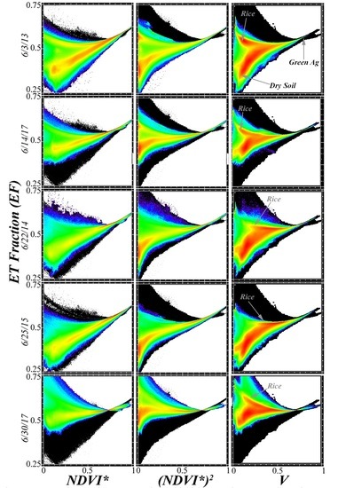
The Mo vs vegetation space, shown in Figure 3b, can be interpreted similarly. In all cases, a clear triangular structure to the space is again evident. All pixels with high vegetation abundances are associated with low Mo, but pixels with low V values can be associated with high Mo (flooded areas & lakes) or low Mo (dry soil & impervious surface). In some scenes, higher-elevation forests in the Sierra Nevada form a distinct cluster in V vs Mo space because they are substantially colder than the rest of the scene. Again, significant differences in internal structure are apparent from metric to metric, with the most complex and informative structures being apparent in the V vs Mo space.
SMA-derived V fraction has long been recognized as a more accurate metric of vegetation abundance than spectral indices like NDVI. Taken together, Figure 3a,b demonstrate how the inaccuracies in NDVI propagate through a simple ET model to clearly result in substantial information loss in estimates of EF and Mo. Evaluation of NDVI*, NDVI*2, and V-based estimates of ET parameters using field measurements from agriculturally met stations, described in the Discussion, confirms that the greater information content of V-based estimates results in improved agreement between satellite and field measurements. While linear and quadratic transformations of NDVI do somewhat linearize the distributions and rescale their ranges, they cannot recover the structure of the bivariate distribution, which is simply not captured by the 2-band normalized difference. When spectral indices are used in more complex ET models, the error propagation may be even more severe.
3.2. Dark Fraction and Albedo
The D fraction provided by SMA also yields information relevant to ET estimation. Bivariate distributions of the D fraction against EF and Mo estimates are shown in the first and third columns of Figure 4. D vs EF spaces show similar overall structures from scene to scene, with a considerably more complex pixel distribution than that of the V vs EF & Mo spaces. Information about the phenological progression of the rice crop is present within this complexity. In early June, rice paddies reside in a consistent cluster at high D and high EF. This cluster is prominently separated from the remainder of the point cloud. As the growing season progresses, D decreases as V increases, and the cluster migrates to join the other green (non-rice) agriculture in the upper left corner of the point cloud at high EF values, but at low D fractions. Dry soil and NPV occupies the lower curvilinear bound of the space, with variable D fraction corresponding to illumination, substrate albedo, roughness, and the fractional cover of the NPV vs soil.
The overall envelope of the D vs Mo distributions (third column of Figure 4) is more triangular than that of the D vs EF distributions. This reflects the propensity for surfaces with high D fractions to have high moisture contents (standing water, saturated soil) or deep shadows. Rice paddies again reside in a consistently isolated cluster in early June, with high values of both D and EF, and migrate toward the remainder of the point cloud as the growing season progresses. Non-rice land cover resides in a more amorphous cluster with intermediate dark fractions and relatively low Mo.
The left and center columns of Figure 5 show the bivariate distribution of D vs T* and α vs T* for each image, respectively. The two distributions have obvious visual similarity, and they give similar information (ρ < −0.98 for all scenes). Clearly, the D fraction well represents broadband shortwave albedo in these images. Pixels with high D fractions and low α values generally have low T* values, generally corresponding to standing water. Pixels with intermediate D fractions or intermediate α, however, can possess any of the full range of T* values. This is because these pixels can correspond to a wide range of land covers, including green crops, forests, dry fields, and impervious surfaces. The two subparallel diagonal limbs in the D vs T* space correspond to variations in crop canopy structural shadow and plant spacing.
3.3. Substrate Fraction, Temperature, and ET
The third complementary piece of information given by the SVD approach is contained in the S fraction. The distributions of S versus EF & Mo are examined in the second and fourth columns of Figure 4. Again, broad similarities in structure are observed between scenes. EF shows a consistent inverse relationship to S, fanning out at higher S values in correspondence to the spectral ambiguity between soil and NPV. In contrast, the relationship between S and Mo is generally triangular, and it has some visual similarities to the relationship between V and Mo, shown in Figure 3b. Pixels with high S values uniformly have low Mo values, accurately representing the low moisture content of bright, dry soils and NPV. However, pixels with low S values can have either high or low Mo values, corresponding to standing water or dense vegetation, respectively. In some scenes, the sporadic clouds intentionally carried through the analysis distort these relationships by yielding spuriously high S values, low T values, and high EF and Mo values. This illustrates the effect that uncorrected atmospheric effects can have on both SMA-derived fractions and ET estimates.
In contrast to the complexity of the V vs T and D vs T distributions, the relationship between S and T is remarkably straightforward in this study area, as shown in the right column of Figure 5. For all 10 June Landsat 8 images in the archive, S fraction shows a simple linear relationship to T. When all the single date spaces are combined into a single multi-date composite space, as shown in Figure 6, this relationship is masked because scene-to-scene variations in air temperature and illumination geometry result in shifts in absolute position of the point cloud in T—but not in its structure. Correlation coefficients for each coincident S vs T image pair, also shown in Figure 6, quantify the strength of this relationship in the 0.7 to 0.9 range, which is substantially stronger than the (negative) relationship between V and T. Because the relationship between S and T is so strong, the relationship between S and V is similar to the relationship between T and V. The potential implications of this observation could be considerable, given that S is quantified using information from the optical bands alone.
4. Discussion
4.1. Application Examples
Figure 7 shows an example of ET estimation using the SVD+T approach on an image from 14 August 2016 in the study area. This image was acquired relatively late in the growing season. In this image, the majority of rice fields have closed canopies, and some are beginning to senesce. Orchards are generally in full leaf at this time, and row crops are in various stages of growth. Rice fields are easily identifiable from the SVD image (top) on the basis of their high V fraction, large field size, and relatively homogenous internal structure. Orchards generally have a lower V fraction and higher S fraction, due to the bare soil that is present between rows of trees. Native vegetation in the wildlife refuges and grasslands is generally senescent at this time of year, resulting in low V fractions and high S fractions. Settlements show considerable complexity, generally resulting in high S and D fractions.
Variations in V and T images are manifest in the EF and Mo images (center and bottom, respectively). EF shows the highest values in the rice fields, and the lowest values in the dry grasslands and fallow fields, consistent with physical expectations. Wildlife refuges show substantial internal structure due to their complex land cover mosaic of water, native plants, and managed vegetation. Orchards and row crops show intermediate EF values. In contrast, the Mo image reveals different spatial patterns. Considerably more internal structure is evident in the rice-growing region in the Mo image than the EF image, consistent with spatial variations in field maturity. Rice in the western portion of this scene was planted earlier than in the east, resulting in more rapid senescence and reduced Mo in the west relative to the east. The spatial structure in the wildlife refuges observed in the EF image is greatly diminished in the Mo image, where the region is characterized by relatively homogenous low Mo values.
Figure 8 presents in greater spatial detail a 24 × 24 km spatial subset, as indicated by the white box in Figure 7. The image shown in Figure 8 was collected earlier in the growing season, on 19 June 2013. The false color image (panel A), together with the coincident thermal image (panel B), allow for broad discrimination among land cover types. The cold, black-to-green large rectilinear fields correspond to flooded paddies with early-stage rice growing in them. Warmer, brighter areas along the Sacramento River channel correspond to row crops and orchards growing in sandier soils. The settlement of Willows, CA is present in the northwest corner of the image, with a complex reflectance signature and elevated temperatures relative to the surrounding agricultural landscape. A wildlife preserve is also present in the southwest corner of the image, characterized by a complex reflectance and temperature mosaic. SVD fractions (panel C) quantify this diversity through the amplitude variations of three continuous fields.
NDVI*, NDVI*2, and V are shown in panels D through F. Relative to V, NDVI* underestimates the vegetative cover in the settlement and wildlife preservation areas, and overestimates it in some areas of rice agriculture. The overestimation in the rice is even more severe for NDVI*2, although the underestimation in the wildlife refuge and settlement areas appears to be less severe. These differences in estimates of fractional vegetation cover then map onto estimates of EF (panels G through I) and Mo (panels J through L) using each metric. The overall spatial pattern of EF does not have extreme variations from metric to metric, although prominent differences are evident within the region of rice agriculture, as well as in the settlement. Mo estimates, on the other hand, are wildly variable. While the spatial pattern of Mo estimated using V appears to match the physical properties of the landscape mosaic, Mo estimated using the spectral indices does not appear to capture even the prominent differences between the dry wildlife refuge and settlement, and the flooded rice paddies. The differences in EF and Mo estimates illustrate the potential sensitivity of ET estimation to the vegetation metrics, and the opportunity for improvement in current estimates that use the SVD approach. While we have used apparent brightness temperature and top of atmosphere reflectance to illustrate the effects of air temperature, future applications could make use of atmospherically corrected surface reflectance and surface temperature Landsat products provided by the USGS.
4.2. Evaluation
One reason this analysis uses the Triangle Method is because both EF and Mo are relative measures of ET, providing information about the spatial distribution of total ET and soil moisture, but not absolute estimates of actual ET flux. This aligns with the goal of the study to provide a novel conceptual framework, within which ET models can be understood and harmonized—rather than proposing a particular predictive model. We principally focus on the relative distributions of data and model parameters across images, in order to (1) show the effect that differences in vegetation metric can have on even simple ET models, and (2) to show the differences and consistencies between S and D fractions, observed T, and estimated EF and Mo.
Despite these caveats, however, comparison of remotely sensed estimates with ground observations of relevant variables can still provide valuable insights. Ideally, direct field measures of actual ET from flux towers and/or lysimeters would be available to provide local calibration and validation constraints. To our knowledge, no such data are available for our region during the 2013–2018 time period that we considered. This unfortunately precludes direct validation.
Agricultural meteorological data do exist in the area, however, in the form of a network of standardized weather stations maintained by the California Irrigation Management Information System (CIMIS). CIMIS stations measure a wide range of micrometeorological variables, including wind speed and direction, air temperature and humidity, solar radiation, and soil temperature. These data are used to provide standardized estimates of ET-relevant derived quantities, including reference ET (ETo). Fortunately, four CIMIS stations are situated within our study area, and two more (Davis and Woodland) are immediately to the south (Figure 9).
The plots at the bottom of Figure 9 compare the time series of CIMIS-measured soil temperature (green) and air temperature (red) in comparison to Landsat-estimated brightness temperature (black) for nine pixels closest to each of the four CIMIS stations located within the study area. While some discrepancies do exist, the Landsat temperatures estimates generally track the upper bound of the CIMIS air temperature to within 3–5 °C. Differences in the accuracy with which Landsat measurements track different stations are likely due to differences in the siting of each station, particularly the spatial homogeneity and land cover of the surrounding landscape.
Figure 10 illustrates the relative ability of EF and Mo estimates based on V, NDVI*, and NDVI*2 to track ground observations. Every available cloud-free Landsat 8 scene in 2017 and 2018 was processed with the same global NDVImax, NDVImin, Tmax, and Tmin values that were used for the rest of the analysis. EF and Mo values for maximally vegetated pixels were then selected from the distributions of (V/NDVI*/NDVI*2) vs (EF/Mo) to represent the conditions that are present at well-watered, densely vegetated CIMIS stations. EF estimates were compared against CIMIS-derived ETo (L) and Mo estimates were compared against (inverted) CIMIS-measured soil temperature (R). EF estimates using V track ETo more closely than EF estimates using NDVI*. EF estimated using NDVI*2 shows high amplitude peaks and oscillations throughout the growing season, which are not present in ground observations. Moderately strong positive correlations (0.7 to 0.9) between EF estimates and individual station ETo records are observed for all metrics. While individual correlations are statistically significant (in all cases, p < 0.001 compared to null hypothesis of 0 correlation), the differences between the correlations are not (p > 0.1 in all cases).
Mo estimates show a similar pattern when compared against ground-based soil T measurements. When the SMA-derived V fraction is used, Mo estimates track the seasonal cycle of soil T remarkably closely. In contrast, Mo estimates using NDVI* and NDVI*2 overestimate Mo at the beginning and end of the growing season. This is in accord with the known superiority of V over NDVI in situations with sparse (early season) or senescent (late season) vegetation. Again, moderately strong positive correlations are observed between Mo estimates and individual station Soil T records for all metrics. Again, individual correlations are statistically significant (in all cases, p < 0.001 compared to null hypothesis of 0 correlation) but differences between the correlations are not (p > 0.1 in all cases). While admittedly indirect, this comparison to the available ground measurements provides additional evidence supporting the improvement, using the SMA-derived V fraction over transformed spectral indices like NDVI* and NDVI*2.
4.3. ET Partitioning
A recent global analysis has shown the partitioning of ET into its primary subcomponents of transpiration (leaf water to air), soil evaporation (soil moisture to air), and interception evaporation (plant surface water to air) to vary widely between common ET models [71]. Further work (published in this Special Issue) specifically shows NDVI to be the input parameter resulting in the greatest sensitivity of total ET estimates generated by the Priestley–Taylor Jet Propulsion Laboratory (PT-JPL) ET model, with substantial nonlinearity [72]. As mentioned in [72], nonlinearities in model formulation may explain this result. In addition, we suggest that another factor potentially contributing to this sensitivity could be the generally nonlinear relationship between the model input parameter (NDVI), and the physical quantity that it is intended to represent (fractional vegetation abundance). This hypothesis could be easily investigated through trials with the simple replacement of NDVI with SMA-estimated V. If the hypothesis is supported and improvement is seen, replacement of NDVI with V could offer a straightforward pathway towards ET model improvement requiring minimal effort.
This opportunity is not unique to the PT-JPL model. Many ET model formulations assume a simple relationship between a biogeophysical landscape quantity, such as fractional vegetation abundance and a spectral index. A robust body of previous work (partially reviewed in the Background section above) has shown SMA to outperform spectral indices in a wide range of environments and spatial resolutions, especially in the case of broadband multispectral imagery. SMA also has the advantage of being grounded in a straightforward physical basis, and it accounts for the effects of soil reflectance, moisture content, and shadow explicitly. In general, it is reasonable to expect that the relationship between the true subpixel areal abundance of land cover and the estimate given by SMA to be more accurate, and scale more linearly, than the estimate that is given by a normalized difference index. Given the ease with which SMA can be implemented into multispectral image processing workflows, and the current prevalence of spectral vegetation indices in ET models, this presents a substantial opportunity for the improvement of remote sensing-based estimation of ET.
Despite their considerable advantages, the linear scaling properties of SMA-derived land cover fractions alone are not likely to resolve all scaling nonlinearities in ET estimation. The effects of other nonlinearities in the ET estimation process, such as surface roughness, are significant, and they can be observed in cases where vegetation parameters scale accurately. The recent work of [73] observes one such system. Using the METRIC model to estimate ET from an open-canopy olive orchard, Ramirez-Cuesta et al. find scaling discrepancies in sensible and latent heat fluxes of up to 24% and 15%, respectively. These differences could not be attributed to albedo or vegetation parameterization of the METRIC model. This work serves to highlight the complexity of the ET estimation problem, and the need for further work on characterizing the relationship between the spatial configuration of the landscape and the scaling of the ET estimates.
4.4. Thermal EM Selection
ET estimation methods that rely on the regional V vs T relation are generally sensitive to the selection of hot and cold thermal endmembers [74,75,76]. As noted by [77], the hot & cold EMs fundamentally set SVAT model boundary conditions, and thus constrain the distribution of possible ET outcomes. Because of this, ET models rooted in the V vs T relation can fundamentally only be as accurate and as consistent as the thermal EMs used in their formulation.
The SVD approach provides users with additional information about potential thermal EMs by providing two additional quantities relating to the land cover of the pixel. This information could be especially useful when considering the choice of hot EM, a particularly important and sensitive point, as noted by [75]. The two parameters of spectral vegetation index and brightness temperature alone are generally insufficient to reliably distinguish between such widely variable materials as asphalt (or other low albedo anthropogenic surfaces), dry NPV (standing or cut crop litter, senesced grass), dry low albedo soil, and dry high albedo soil. However, by adding the S and D fraction information, these materials can be readily distinguished using their position in a 4-dimensional parameter space. This enhanced ability to discriminate between potential hot EM materials could support attempts to improve the consistency and accuracy of thermal EM selection.
4.5. Clustering in Fraction vs ET Parameter Space
The structure of the SVD fraction vs ET parameter spaces is a key component of this analysis. Both broad consistencies and illuminating differences are present between images in each space. Clustering in these spaces, indicative of landscape subsets with similar land cover and ET combinations, can be useful for mapping distinct land cover types. For example, the flooded rice paddies common in the study area are shown in Figure 3, Figure 4 and Figure 5 as occupying a distinct position in each of the S, V, and D vs T, EF and Mo spaces. The position of these paddies relative to the other points in the space migrates throughout the growing season, resulting in a set of trajectories that are characteristic of rice paddies that are distinct from those of other types of crops, grasslands, or non-agricultural vegetation.
Clustering in the feature space is also the foundation for discrete image classification. By contributing an additional (although not independent) set of basis vectors for the multispectral feature space, the ET parameter estimates offer an additional opportunity to help the statistical classification algorithms to resolve distinctions between the spectral–thermal properties of different land covers. Especially when approached from a multitemporal framework [78], this information could potentially be used to improve image classification algorithms used for the mapping and monitoring of both human-modified and wilderness landscapes.
4.6. The SVD Approach as a Unifying Framework
The bivariate parameter spaces shown in Figure 2, Figure 3, Figure 4, Figure 5 and Figure 6, and the examples shown in Figure 7 and Figure 8, illustrate the value of SMA with globally standardized SVD EMs as a unifying framework for two complementary approaches to ET investigation: the V vs T relationship and the α vs T relationship. Figure 2 and Figure 3 illustrate the ET-specific advantages of using V over the currently used metrics, such as NDVI* and NDVI*2, on the basis of the enhanced clustering and structure in the V vs T, EF, and Mo distributions. These advantages, in addition to previously demonstrated scaling and background suppression properties, advocate for the use of SMA-derived V fraction in ET studies.
In addition to V, the SVD+T approach simultaneously retrieves information on two other factors influencing ET; fractional soil exposure and soil moisture. The left and center columns of Figure 5 show this information from the D fraction to be highly similar to (inverted) broadband shortwave albedo (ρ < −0.98 for all scenes). The right column of Figure 5 and Figure 6 show that S fractions are strongly linearly related to T, at least in the June imagery in this study area. While this relationship does have a strong physical basis, more investigation is warranted, to confirm its generality in other environments and seasons. However, the agricultural and soil complexity in the Sacramento Valley suggest that the relationship may hold in other agricultural environments. By synthesizing the contributions of both vegetation abundance and albedo, the SVD+T approach presents a unified framework for considering two of the main branches of the ET literature.
The focus of this analysis on a single study area may beg the question of the generality of the results. While the persistence of the feature space structure over several years is encouraging, it does not guarantee that the method will perform as well in other environments. However, the global analysis of [79] did find a remarkable similarity of structure in the SVD fraction vs T spaces of 24 diverse urban-rural gradients spanning a very wide range of environments and land cover types. While the abundance of impervious surface in those environments complicates interpretation in terms of ET, a simple comparison of the SVD vs T spaces from [79] with those in this analysis shows obvious similarities. The strong linearity of the S vs T space observed in the California study area is not a general feature in the global analysis, although it does appear in some examples containing abundant agriculture (e.g., Calgary, Essen & Cairo). An intercomparison of a diverse sample of agricultural areas worldwide is the focus of a separate study.
Finally, the clustering that is apparent in the S, V, & D fractions versus T*, Mo, and EF spaces suggests that these spaces could provide the basis for either continuous or discrete classifications of crop types and growth stages for agricultural monitoring. This approach could be particularly effective when combined with spatiotemporal analysis of phenological information derived from multitemporal observations, as proposed by [78]. In addition, once planned global hyperspectral missions become a reality, the SVD framework could also be integrated with targeted narrowband approaches such as that of [80].
5. Conclusions
The primary purpose of this study is to demonstrate the potential for spectral mixture analysis (SMA) based on globally standardized substrate, vegetation, and dark (SVD) endmembers (EMs) to provide a comprehensive, integrated framework for ET parameter estimation. The SVD approach yields complementary continuous field estimates of the subpixel fractional abundance of each EM. V fraction is an accurate, linearly scalable metric for vegetation abundance. D fraction is the linear complement to albedo. The linear tradeoff between S and D fractions provides information about the soil and NPV exposure, tillage conditions, and moisture content. Using the Triangle Method as an example model, the results of this analysis show substantially enhanced clustering in both the ET fraction (EF) and moisture availability (Mo) estimates, based on the V fraction, compared to the generally used NDVI* or NDVI*2. Replacing NDVI-based vegetation metrics with the standardized vegetation fraction eliminates a known nonlinearity and allows for pixel-based fractions to be downscaled and vicariously validated with higher resolution imagery when available. EF and Mo that are estimated using V also track field measurements of reference ET & soil temperature more closely than EF & Mo estimated using NDVI* or NDVI*2. Using the coefficients of [70], we show the D vs T relationship to be very similar to broadband shortwave albedo (α) vs T. Finally, we show S to have a consistent linear relationship with T, at least in this study area during peak growing and insolation season. SMA allows globally standardized S, V, and D fractions to be estimated simultaneously, with high accuracy and at trivial computational cost. The implications of such a unified framework for the standardization and accuracy improvement of ET models could be considerable.
Author Contributions
Conceptualization, D.S. and C.S.; Formal Analysis, D.S.; Funding Acquisition, D.S. and C.S.; Investigation, D.S. and C.S.; Methodology, D.S. and C.S.; Supervision, C.S.; Writing—Original Draft, D.S.; Writing—Review & Editing, D.S. and C.S.
Funding
Work done by D.S. was conducted with Government support under FA9550-11-C-0028, and awarded by the Department of Defense, Air Force Office of Scientific Research, National Defense Science and Engineering Graduate (NDSEG) Fellowship, 32 CFR 168a. C.S. gratefully acknowledges the support of the NASA Multi-Source Land Imaging Program (grant NNX15AT65G).
Acknowledgments
The authors thank three anonymous reviewers and editor M. McCabe for their constructive comments. D.S. thanks Carl and Victor Akers for inspiration and insight.
Conflicts of Interest
The authors declare no conflict of interest.
References
- Miralles, D.G.; van den Berg, M.J.; Gash, J.H.; Parinussa, R.M.; de Jeu, R.A.M.; Beck, H.E.; Holmes, T.R.H.; Jiménez, C.; Verhoest, N.E.C.; Dorigo, W.A.; et al. El Niño–La Niña cycle and recent trends in continental evaporation. Nat. Clim. Chang. 2013, 4, 122–126. [Google Scholar] [CrossRef]
- Miralles, D.G.; Van Den Berg, M.J.; Teuling, A.J.; De Jeu, R.A.M. Soil moisture-temperature coupling: A multiscale observational analysis. Geophys. Res. Lett. 2012, 39. [Google Scholar] [CrossRef] [Green Version]
- Miralles, D.G.; De Jeu, R.A.M.; Gash, J.H.C.; Holmes, T.R.H.; Dolman, A.J. Magnitude and variability of land evaporation and its components at the global scale. Hydrol. Earth Syst. Sci. 2011, 15, 967–981. [Google Scholar] [CrossRef] [Green Version]
- Zhang, Y.; Peña-Arancibia, J.L.; McVicar, T.R.; Chiew, F.H.S.; Vaze, J.; Liu, C.; Lu, X.; Zheng, H.; Wang, Y.; Liu, Y.Y.; et al. Multi-decadal trends in global terrestrial evapotranspiration and its components. Sci. Rep. 2016, 6, 19124. [Google Scholar] [PubMed] [Green Version]
- Jackson, R.D.; Reginato, R.J.; Idso, S.B. Wheat canopy temperature: A practical tool for evaluating water requirements. Water Resour. Res. 1977, 13, 651–656. [Google Scholar] [CrossRef]
- Jackson, R.D.; Idso, S.B.; Reginato, R.J.; Pinter, P.J., Jr. Canopy temperature as a crop water stress indicator. Water Resour. Res. 1981, 17, 1133–1138. [Google Scholar] [CrossRef]
- Idso, S.B.; Jackson, R.D.; Reginato, R.J. Remote-Sensing of Crop Yields. Science 1977, 196, 19–25. [Google Scholar] [CrossRef] [PubMed]
- Allen, R.G.; Tasumi, M.; Morse, A.; Trezza, R. A Landsat-based energy balance and evapotranspiration model in Western US water rights regulation and planning. Irrig. Drain. Syst. 2005, 19, 251–268. [Google Scholar] [CrossRef]
- Bastiaanssen, W.; Noordman, E.J.M.; Pelgrum, H.; Davids, G.; Thoreson, B.P.; Allen, R.G. SEBAL Model with Remotely Sensed Data to Improve Water-Resources Management under Actual Field Conditions. J. Irrig. Drain. Eng. 2005, 131, 85–93. [Google Scholar] [CrossRef]
- Farahani, H.; Howell, T.A.; Shuttleworth, W.J.; Bausch, W.C. Evapotranspiration: Progress in Measurement and Modeling in Agriculture. Trans. ASABE 2007, 50, 1627–1638. [Google Scholar] [CrossRef] [Green Version]
- Fisher, J.B.; Whittaker, R.J.; Malhi, Y. ET come home: Potential evapotranspiration in geographical ecology. Glob. Ecol. Biogeogr. 2011, 20, 1–18. [Google Scholar] [CrossRef]
- Gaston, K.J. Global patterns in biodiversity. Nature 2000, 405, 220–227. [Google Scholar] [CrossRef] [PubMed]
- Shafroth, P.B.; Brown, C.A.; Merritt, D.M. Saltcedar and Russian olive control demonstration act science assessment. In Scientific Investigations Report 2009-5247; U.S. Geologic Survey: Reston, VA, USA, 2010. [Google Scholar]
- Anderson, M.; Allen, R.G.; Morse, A.; Kustas, W.P. Use of Landsat thermal imagery in monitoring evapotranspiration and managing water resources. Remote Sens. Environ. 2012, 122, 50–65. [Google Scholar] [CrossRef]
- Allen, R.G.; Tasumi, M.; Trezza, R. Satellite-based energy balance for mapping evapotranspiration with internalized calibration (METRIC) Model. J. Irrig. Drain. Eng. 2007, 133, 380–394. [Google Scholar] [CrossRef]
- Bastiaanssen, W.; Menenti, M.; Feddes, R.A.; Holtslag, A.A.M. A remote sensing surface energy balance algorithm for land (SEBAL). 1. Formulation. J. Hydrol. 1998, 212–213, 198–212. [Google Scholar] [CrossRef]
- Carlson, T.N.; Boland, F.E. Analysis of urban-rural canopy using a surface heat flux/temperature model. J. Appl. Meteorol. 1978, 17, 998–1013. [Google Scholar] [CrossRef]
- Moran, M.S.; Clarke, T.R.; Inoue, Y.; Vidal, A. Estimating crop water deficit using the relation between surface-air temperature and spectral vegetation index. Remote Sens. Environ. 1994, 49, 246–263. [Google Scholar] [CrossRef]
- Wang, L.; Good, S.P.; Caylor, K.K. Global synthesis of vegetation control on evapotranspiration partitioning. Geophys. Res. Lett. 2014, 41, 6753–6757. [Google Scholar] [CrossRef] [Green Version]
- Menenti, M.; Bastiaanssen, W.; Van Eick, D.; El Karim, M.A.A. Linear relationships between surface reflectance and temperature and their application to map actual evaporation of groundwater. Adv. Space Res. 1989, 9, 165–176. [Google Scholar] [CrossRef]
- Ångström, A. The Albedo of Various Surfaces of Ground. Geogr. Ann. 1925, 7, 323–342. [Google Scholar] [CrossRef]
- Idso, S.B.; Jackson, R.D.; Reginato, R.J.; Kimball, B.A.; Nakayama, F.S. The dependence of bare soil albedo on soil water content. J. Appl. Meteorol. 1975, 14, 109–113. [Google Scholar] [CrossRef]
- Matthias, A.D.; Fimbres, A.; Sano, E.E.; Post, D.F.; Accioly, L.; Batchily, A.K.; Ferreira, L.G. Surface roughness effects on soil albedo. Soil Sci. Soc. Am. J. 2000, 64, 1035–1041. [Google Scholar] [CrossRef]
- Roerink, G.J.; Su, Z.; Menenti, M. S-SEBI: A simple remote sensing algorithm to estimate the surface energy balance. Phys. Chem. Earth Part B Hydrol. Ocean. Atmos. 2000, 25, 147–157. [Google Scholar] [CrossRef]
- Merlin, O.; Chirouze, J.; Olioso, A.; Jarlan, L.; Chehbouni, G.; Boulet, G. An image-based four-source surface energy balance model to estimate crop evapotranspiration from solar reflectance/thermal emission data (SEB-4S). Agric. For. Meteorol. 2014, 184, 188–203. [Google Scholar] [CrossRef] [Green Version]
- Jiang, L.; Islam, S. A methodology for estimation of surface evapotranspiration over large areas using remote sensing observations. Geophys. Res. Lett. 1999, 26, 2773–2776. [Google Scholar] [CrossRef] [Green Version]
- Kustas, W.P.; Norman, J.M.; Anderson, M.C.; French, A.N. Estimating subpixel surface temperatures and energy fluxes from the vegetation index-radiometric temperature relationship. Remote Sens. Environ. 2003, 85, 429–440. [Google Scholar] [CrossRef]
- Elmore, A.J.; Mustard, J.F.; Manning, S.J.; Lobell, D.B. Quantifying vegetation change in semiarid environments: Precision and accuracy of spectral mixture analysis and the normalized difference vegetation index. Remote Sens. Environ. 2000, 73, 87–102. [Google Scholar] [CrossRef]
- Price, J.C. Using spatial context in satellite data to infer regional scale evapotranspiration. IEEE Trans. Geosci. Remote Sens. 1990, 28, 940–948. [Google Scholar] [CrossRef] [Green Version]
- Small, C. Estimation of urban vegetation abundance by spectral mixture analysis. Int. J. Remote Sens. 2001, 22, 1305–1334. [Google Scholar] [CrossRef] [Green Version]
- Smith, M.O.; Ustin, S.L.; Adams, J.B.; Gillespie, A.R. Vegetation in deserts: I. A regional measure of abundance from multispectral images. Remote Sens. Environ. 1990, 31, 1–26. [Google Scholar] [CrossRef]
- Small, C.; Milesi, C. Multi-scale standardized spectral mixture models. Remote Sens. Environ. 2013, 136, 442–454. [Google Scholar] [CrossRef]
- Choudhury, B.J.; Ahmed, N.U.; Idso, S.B.; Reginato, R.J.; Daughtry, C.S. Relations between evaporation coefficients and vegetation indices studied by model simulations. Remote Sens. Environ. 1994, 50, 1–17. [Google Scholar] [CrossRef]
- Carlson, T.N. An Overview of the “Triangle Method” for Estimating Surface Evapotranspiration and Soil Moisture from Satellite Imagery. Sensors 2007, 7, 1612–1629. [Google Scholar] [CrossRef]
- Carlson, T.N.; Ripley, D.A. On the relation between NDVI, fractional vegetation cover, and leaf area index. Remote Sens. Environ. 1997, 62, 241–252. [Google Scholar] [CrossRef]
- Sun, H. A Two-Source Model for Estimating Evaporative Fraction (TMEF) Coupling Priestley-Taylor Formula and Two-Stage Trapezoid. Remote Sens. 2016, 8, 248. [Google Scholar] [CrossRef]
- Li, G.; Jing, Y.; Wu, Y.; Zhang, F.; Li, G.; Jing, Y.; Wu, Y.; Zhang, F. Improvement of Two Evapotranspiration Estimation Models Using a Linear Spectral Mixture Model over a Small Agricultural Watershed. Water 2018, 10, 474. [Google Scholar] [CrossRef]
- Adams, J.B.; Smith, M.O.; Johnson, P.E. Spectral mixture modeling: A new analysis of rock and soil types at the Viking Lander 1 site. J. Geophys. Res. Solid Earth 1986, 91, 8098–8112. [Google Scholar] [CrossRef]
- Gillespie, A.R.; Smith, M.O.; Adams, J.B.; Willis, S.C.; Fischer, A.F.; Sabol, D.E. Interpretation of residual images: Spectral mixture analysis of AVIRIS images, Owens Valley, California. In Annual JPL Airborne Visible/Infrared Imaging Spectrometer (AVIRIS) Workshop; NASA Jet Propulsion Laboratory: Pasadena, CA, USA, 1990; Volume 2, pp. 54–90. [Google Scholar]
- Smith, M.O.; Johnson, P.E.; Adams, J.B. Quantitative determination of mineral types and abundances from reflectance spectra using principal components analysis. J. Geophys. Res. Solid Earth 1985, 90, C797–C804. [Google Scholar] [CrossRef]
- Baldocchi, D.; Krebs, T.; Leclerc, M.Y. “Wet/dry Daisyworld”: A conceptual tool for quantifying the spatial scaling of heterogeneous landscapes and its impact on the subgrid variability of energy fluxes. Tellus B Chem. Phys. Meteorol. 2005, 57, 175–188. [Google Scholar] [CrossRef]
- Brunsell, N.; Gillies, R. Length Scale Analysis of Surface Energy Fluxes Derived from Remote Sensing. J. Hydrometeorol. 2003, 4, 1212–1219. [Google Scholar] [CrossRef] [Green Version]
- McCabe, M.F.; Wood, E.F. Scale influences on the remote estimation of evapotranspiration using multiple satellite sensors. Remote Sens. Environ. 2006, 105, 271–285. [Google Scholar] [CrossRef]
- Brunsell, N.; Anderson, M. Characterizing the multi–scale spatial structure of remotely sensed evapotranspiration with information theory. Biogeosciences 2011, 8, 2269–2280. [Google Scholar] [CrossRef] [Green Version]
- Ershadi, A.; McCabe, M.F.; Evans, J.P.; Walker, J.P. Effects of spatial aggregation on the multi-scale estimation of evapotranspiration. Remote Sens. Environ. 2013, 131, 51–62. [Google Scholar] [CrossRef]
- Sharma, V.; Kilic, A.; Irmak, S. Impact of scale/resolution on evapotranspiration from Landsat and MODIS images. Water Resour. Res. 2016, 52, 1800–1819. [Google Scholar] [CrossRef] [Green Version]
- Small, C. The Landsat ETM+ spectral mixing space. Remote Sens. Environ. 2004, 93, 1–17. [Google Scholar] [CrossRef]
- Sousa, D.; Small, C. Global cross-calibration of Landsat spectral mixture models. Remote Sens. Environ. 2017, 192. [Google Scholar] [CrossRef]
- Carlson, T.N.; Gillies, R.; Perry, E. A method to make use of thermal infrared temperature and NDVI measurements to infer surface soil water content and fractional vegetation cover. Remote Sens. Rev. 1994, 9, 161–173. [Google Scholar] [CrossRef]
- Anderson, M.; Norman, J.; Mecikalski, J.R.; Torn, R.D.; Kustas, W.P.; Basara, J.B. A multiscale remote sensing model for disaggregating regional fluxes to micrometeorological scales. J. Hydrometeorol. 2004, 5, 343–363. [Google Scholar] [CrossRef]
- Anderson, M.; Kustas, W.; Norman, J.; Hain, C.; Mecikalski, J.; Schultz, L.; González-Dugo, M.; Cammalleri, C.; D’Urso, G.; Pimstein, A. Mapping daily evapotranspiration at field to continental scales using geostationary and polar orbiting satellite imagery. Hydrol. Earth Syst. Sci. 2011, 15, 223–239. [Google Scholar] [CrossRef] [Green Version]
- Anderson, M.C.; Norman, J.M.; Diak, G.R.; Kustas, W.P.; Mecikalski, J.R. A two-source time-integrated model for estimating surface fluxes using thermal infrared remote sensing. Remote Sens. Environ. 1997, 60, 195–216. [Google Scholar] [CrossRef]
- Nieto, H.; Kustas, W.P.; Torres-Rúa, A.; Alfieri, J.G.; Gao, F.; Anderson, M.C.; White, W.A.; Song, L.; Alsina, M.; Prueger, J.H.; et al. Evaluation of TSEB turbulent fluxes using different methods for the retrieval of soil and canopy component temperatures from UAV thermal and multispectral imagery. Irrig. Sci. 2018, 1–18. [Google Scholar] [CrossRef]
- Yang, J.; Wang, Y. Estimating evapotranspiration fraction by modeling two-dimensional space of NDVI/albedo and day–night land surface temperature difference: A comparative study. Adv. Water Resour. 2011, 34, 512–518. [Google Scholar] [CrossRef]
- Galleguillos, M.; Jacob, F.; Prévot, L.; French, A.; Lagacherie, P. Comparison of two temperature differencing methods to estimate daily evapotranspiration over a Mediterranean vineyard watershed from ASTER data. Remote Sens. Environ. 2011, 115, 1326–1340. [Google Scholar] [CrossRef]
- Petropoulos, G.; Carlson, T.; Wooster, M.; Islam, S. A review of Ts/VI remote sensing based methods for the retrieval of land surface energy fluxes and soil surface moisture. Prog. Phys. Geogr. 2009, 33, 224–250. [Google Scholar] [CrossRef]
- Carter, C.; Liang, S. Comprehensive evaluation of empirical algorithms for estimating land surface evapotranspiration. Agric. For. Meteorol. 2018, 256–257, 334–345. [Google Scholar] [CrossRef]
- Kalma, J.D.; McVicar, T.R.; McCabe, M.F. Estimating land surface evaporation: A review of methods using remotely sensed surface temperature data. Surv. Geophys. 2008, 29, 421–469. [Google Scholar] [CrossRef]
- Johnson, P.E.; Smith, M.O.; Taylor-George, S.; Adams, J.B. A semiempirical method for analysis of the reflectance spectra of binary mineral mixtures. J. Geophys. Res. Solid Earth 1983, 88, 3557–3561. [Google Scholar] [CrossRef]
- Singer, R.B. Near-infrared spectral reflectance of mineral mixtures: Systematic combinations of pyroxenes, olivine, and iron oxides. J. Geophys. Res. Solid Earth 1981, 86, 7967–7982. [Google Scholar] [CrossRef]
- Singer, R.B.; McCord, T.B. Mars-large scale mixing of bright and dark surface materials and implications for analysis of spectral reflectance. In Lunar and Planetary Science Conference Proceedings; Pergamon Press: Houston, TX, USA, 1979; pp. 1835–1848. [Google Scholar]
- Kauth, R.J.; Thomas, G.S. The Tasseled Cap—A graphic description of the spectral-temporal development of agricultural crops as seen by Landsat. In Proceedings of the Symposium on Machine Processing of Remotely Sensed Data; Purdue University: West Lafayette, Indiana, 1976; pp. 4B41–4B51. [Google Scholar]
- Small, C. Multisource imaging of urban growth and infrastructure using Landsat, Sentinel and SRTM. In NASA Landsat-Sentinel Science Team Meeting; NASA: Rockville, MD, USA, 2018. [Google Scholar]
- Sousa, D.; Small, C. Multisensor analysis of spectral dimensionality and soil diversity in the great central valley of California. Sensors 2018, 18. [Google Scholar] [CrossRef]
- USGS Global Visualization Viewer (GloVis). Available online: https://glovis.usgs.gov/ (accessed on 4 December 2018).
- United States Geological Survey (USGS). Landsat 8 Data Users Handbook, Version 2.0; USGS: Sioux Falls, SD, USA, 2016.
- Gerace, A.; Montanaro, M. Derivation and validation of the stray light correction algorithm for the thermal infrared sensor onboard Landsat 8. Remote Sens. Environ. 2017, 191, 246–257. [Google Scholar] [CrossRef]
- Montanaro, M.; Gerace, A.; Lunsford, A.; Reuter, D. Stray Light Artifacts in Imagery from the Landsat 8 Thermal Infrared Sensor. Remote Sens. 2014, 6, 10435–10456. [Google Scholar] [CrossRef] [Green Version]
- Gutman, G.; Ignatov, A. The derivation of the green vegetation fraction from NOAA/AVHRR data for use in numerical weather prediction models. Int. J. Remote Sens. 1998, 19, 1533–1543. [Google Scholar] [CrossRef]
- Liang, S. Narrowband to broadband conversions of land surface albedo: I. Algorithms. Remote Sens. Environ. 2001, 76, 213–238. [Google Scholar] [CrossRef]
- Talsma, C.J.; Good, S.P.; Jimenez, C.; Martens, B.; Fisher, J.B.; Miralles, D.G.; McCabe, M.F.; Purdy, A.J. Partitioning of evapotranspiration in remote sensing-based models. Agric. For. Meteorol. 2018, 260–261, 131–143. [Google Scholar] [CrossRef]
- Talsma, C.J.; Good, S.P.; Miralles, D.G.; Fisher, J.B.; Martens, B.; Jimenez, C.; Purdy, A.J. Sensitivity of Evapotranspiration Components in Remote Sensing-Based Models. Remote Sens. 2018, 10, 1601. [Google Scholar] [CrossRef]
- Ramírez-Cuesta, J.M.; Allen, R.G.; Zarco-Tejada, P.J.; Kilic, A.; Santos, C.; Lorite, I.J. Impact of the spatial resolution on the energy balance components on an open-canopy olive orchard. Int. J. Appl. Earth Obs. Geoinf. 2019, 74, 88–102. [Google Scholar] [CrossRef]
- Long, D.; Singh, V.P. Assessing the impact of end-member selection on the accuracy of satellite-based spatial variability models for actual evapotranspiration estimation. Water Resour. Res. 2013, 49, 2601–2618. [Google Scholar] [CrossRef] [Green Version]
- Timmermans, W.J.; Kustas, W.P.; Anderson, M.C.; French, A.N. An intercomparison of the surface energy balance algorithm for land (SEBAL) and the two-source energy balance (TSEB) modeling schemes. Remote Sens. Environ. 2007, 108, 369–384. [Google Scholar] [CrossRef]
- Long, D.; Singh, V.P.; Li, Z.-L. How sensitive is SEBAL to changes in input variables, domain size and satellite sensor? J. Geophys. Res. Atmos. 2011, 116. [Google Scholar] [CrossRef] [Green Version]
- Carlson, T.N. Triangle Models and Misconceptions. Int. J. Remote Sens. Appl. 2013, 3, 155–158. [Google Scholar]
- Sousa, D.; Small, C. Mapping and Monitoring Rice Agriculture with Multisensor Temporal Mixture Models. Remote Sens. 2018. submitted. [Google Scholar]
- Small, C. Comparative analysis of urban reflectance and surface temperature. Remote Sens. Environ. 2006, 104, 168–189. [Google Scholar] [CrossRef]
- Marshall, M.; Thenkabail, P.; Biggs, T.; Post, K. Hyperspectral narrowband and multispectral broadband indices for remote sensing of crop evapotranspiration and its components (transpiration and soil evaporation). Agric. For. Meteorol. 2016, 218–219, 122–134. [Google Scholar] [CrossRef]
Figure 1.
True color (UL), false color (UR), fraction abundance (LL) and thermal (LR) images of a diverse northern CA landscape as imaged by Landsat 8 on 19 June 2013. Green fields are generally distinct from fallow fields and grasslands in the visible, but infrared bands shown in the false color composite allow superior discrimination. At this time of year, nearly all flooded fields are rice and nearly all green, not flooded fields are row crops & orchards. S, V, D subpixel abundances are estimated using a 3 EM spectral mixture model. Visual agreement between the S fraction and T images suggests that regions dominated by S fraction are generally hotter than regions dominated by V or D fractions.

Figure 2.
Vegetation metric comparison. L: Raw and transformed Normalized Difference Vegetation Index (NDVI, y-axis) vs SMA-derived vegetation fraction (V, x-axis). All three indices overestimate V at intermediate values and roll-off at high values. R: Bivariate distributions of vegetation metrics vs T* all form triangular distributions. However, considerably more structure is evident in the V vs T* distributions than in the index distributions. In early June (top rows), flooded, young rice paddies form a cluster in the V vs T* distributions that is not distinguished by either index, illustrating the inaccuracy of NDVI for sparse vegetation.

Figure 3.
(a) Vegetation metrics vs EF. Regions with high vegetation cover collapse into a tight range of EF. Regions with low vegetation can have high or low EF. For images earlier in June, the abundance of flooded rice paddies results in a cluster at high EF but low T. This cluster migrates to higher V later in June as the rice canopy fills. Again, NDVI* shows the least structure, NDVI*2 is intermediate, and V shows the most structure. (b) Vegetation metrics vs Mo. Regions with high vegetation cover converge into a tight range of low Mo. Regions with low cover can have high or low Mo. In some scenes, forests at higher elevation in the NE corner of the image are colder than that rest of the image and so record anomalously high Mo. With V, the rice paddy cluster is again separate in early June, then moves to high V and low Mo values as the canopy fills. This cluster is barely distinguishable, and the structure much less clear, using either spectral index.


Figure 4.
Dark and Substrate Fractions vs EF and Mo. Corresponding α vs EF and Mo spaces are not shown because nearly indistinguishable from the mirror image of the D vs EF and Mo spaces. The rice paddy cluster is present in both D vs EF and D vs Mo spaces, but only weakly in S vs Mo. High EF values are partitioned between green (non-rice) agriculture at low D & low S values and rice paddies at high D and low S values. D vs Mo distributions generally show increasing Mo with increasing D. S vs EF and Mo distributions show decreasing EF and Mo with increasing S.

Figure 5.
Dark fraction (D), albedo (α), and Substrate (S) vs normalized temperature (T*). The D vs T* relation is similar to the α vs T* relation (with a sign flip). In contrast, the S vs T relation is highly linear. Pixels which are cooler than the main S vs T relation are generally covered with NPV and pixels hotter generally correspond to low albedo soils.

Figure 6.
Composite relationship between S and T. Left: A consistent linear relationship between S and T is observed for nearly every June scene in the Landsat 8 archive, but the composite space of all 10 acquisitions is less obviously linear because significant image-to-image variability exists in air temperature. Right: Correlation between coincident S, V and T images for each date. The observed (+) correlation between S and T is stronger in every case than the well-known (-) correlation between V and T. Because the S vs T correlation is so strong, the S vs V and T vs V correlations are very similar.

Figure 7.
S, V & D fractions, along with EF & Mo, for a sample 15 × 50 km area imaged on 14 August 2016. Flooded paddies have high V and high Mo and EF. Fields in the western half of the image were planted earlier than in the east and have started to senesce, resulting in lower Mo. Orchards have low EF and Mo. The wildlife refuge is complex, with both high and low EF and Mo. Landsat 8 resolves heterogeneity both within individual fields as well as across the valley. The white box shows the spatial subset used for Figure 8.

Figure 8.
Example ET comparison. Landsat 8 collected coincident optical (A) and thermal (B) imagery on 19 June 2013. SVD fraction image (C) reveals substantial spatial heterogeneity in agricultural and preserved lands. NDVI* (D) and NDVI*2 (E) images show substantial differences from each other and from V (F). EF estimates using the three vegetation metrics (G–I) show similar overall patterns, but notable differences within agricultural areas. Differences in Mo (J–L) estimates are even more profound.

Figure 9.
Four met stations are maintained in the study area by the California Irrigation Management Information System (CIMIS). Two more stations exist just to the south of the area. Air temperatures (red) are generally higher and more variable than soil (green). Durham, Verona, & Biggs records are generally similar, with Landsat-observed brightness temperatures (black) at the warm bound of the envelope of air temperatures. The Williams station (installed mid 2016) has substantially lower air, but similar soil and brightness temperatures, to the other stations.

Figure 10.
Comparison to ground observations. EF (L) and Mo estimates (R) from maximally-vegetated pixels from all cloud-free observations from 2017 and 2018 are compared against CIMIS data. Strong seasonality is evident in al observations. EF from SMA-derived V fraction tracks CIMIS-estimated ETo more accurately than EF from NDVI*. EF from NDVI*2 shows pronounced oscillations which are not present in the CIMIS data. Mo from SMA-derived V fraction tracks soil T much more accurately than Mo from NDVI* or NDVI*2. Mo estimated using the spectral indices does not capture the curvature of the seasonal peak, likely as a result of effects of soil background reflectance in pixels with sparse (early season) and senescent (late season) vegetation.


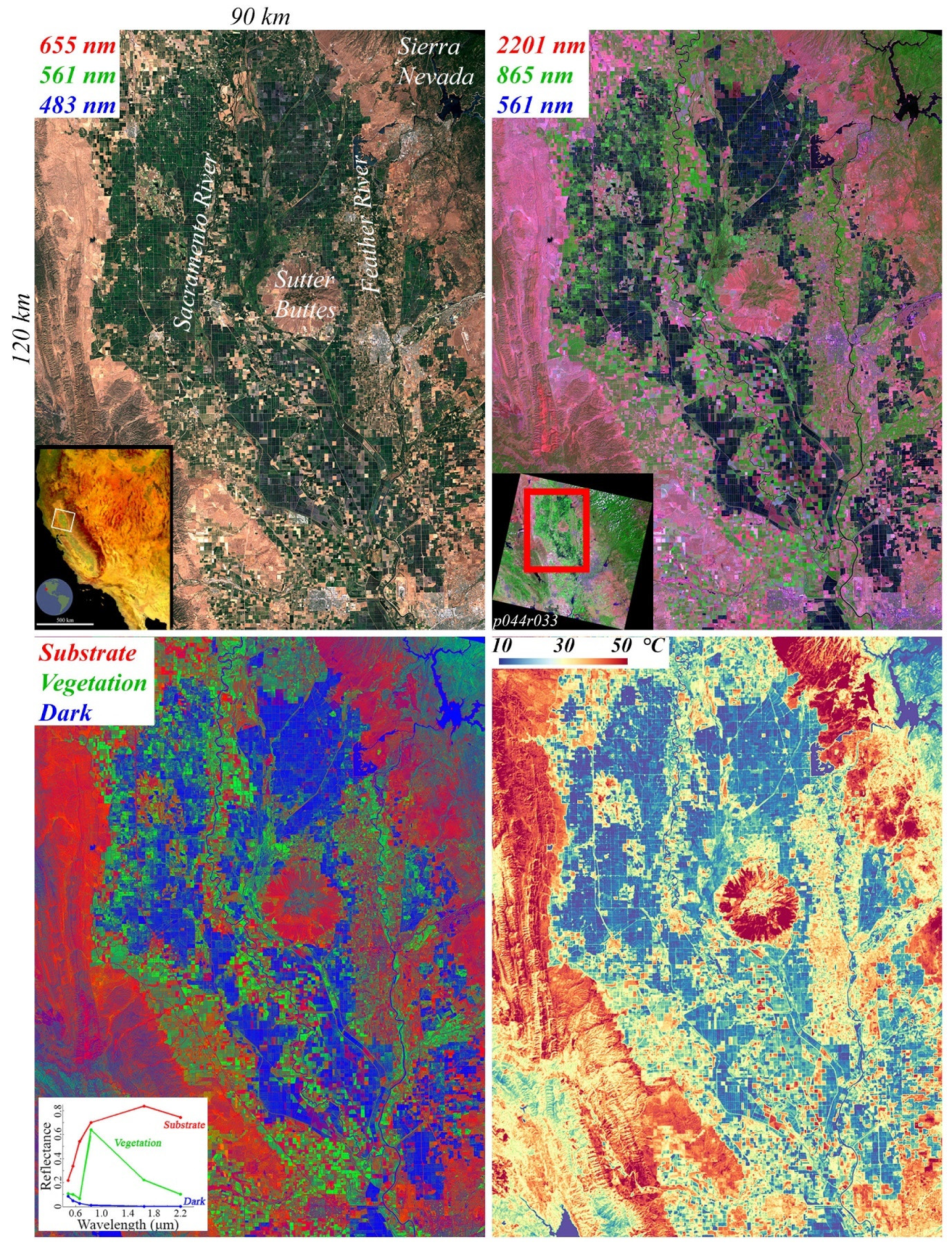
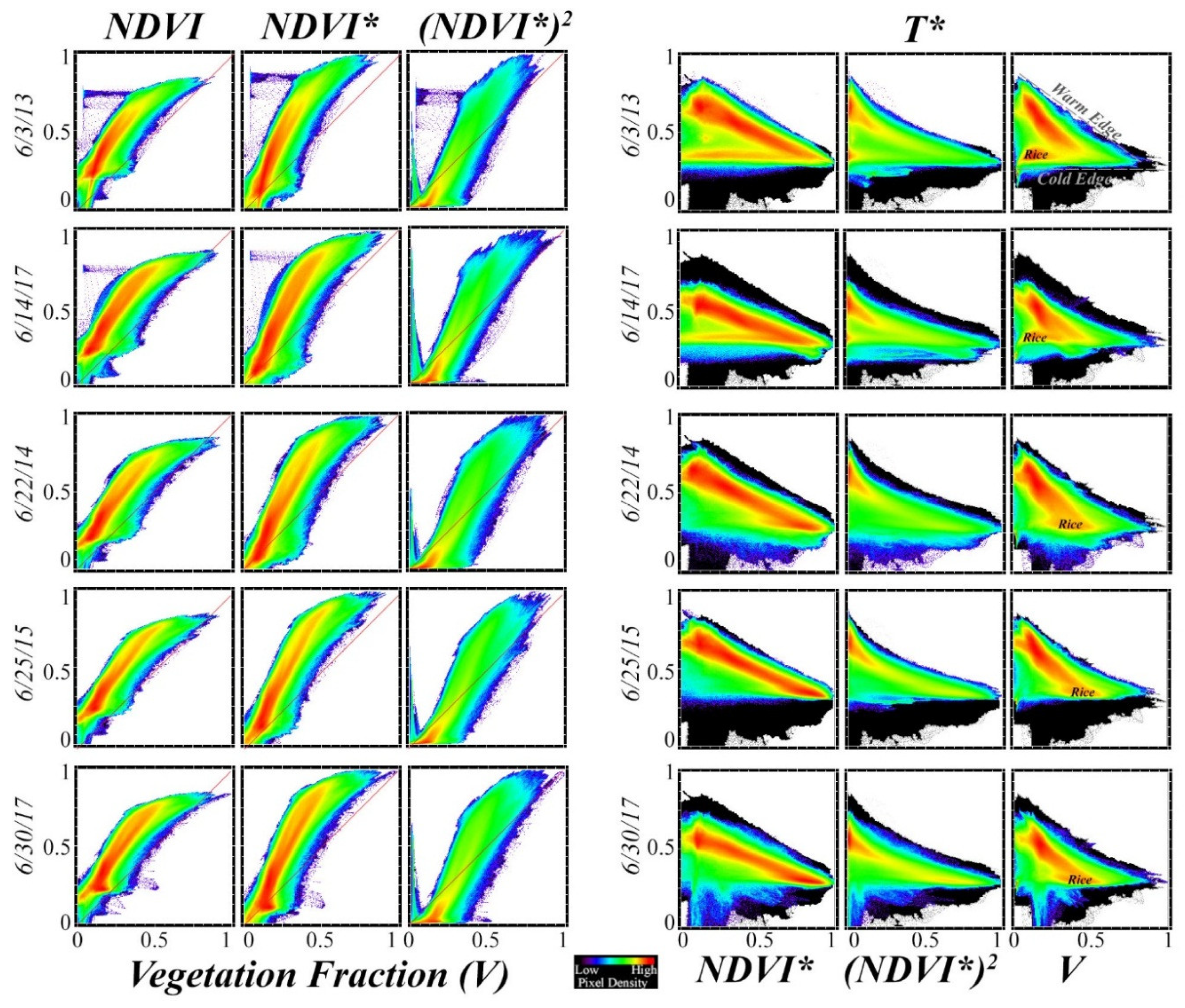
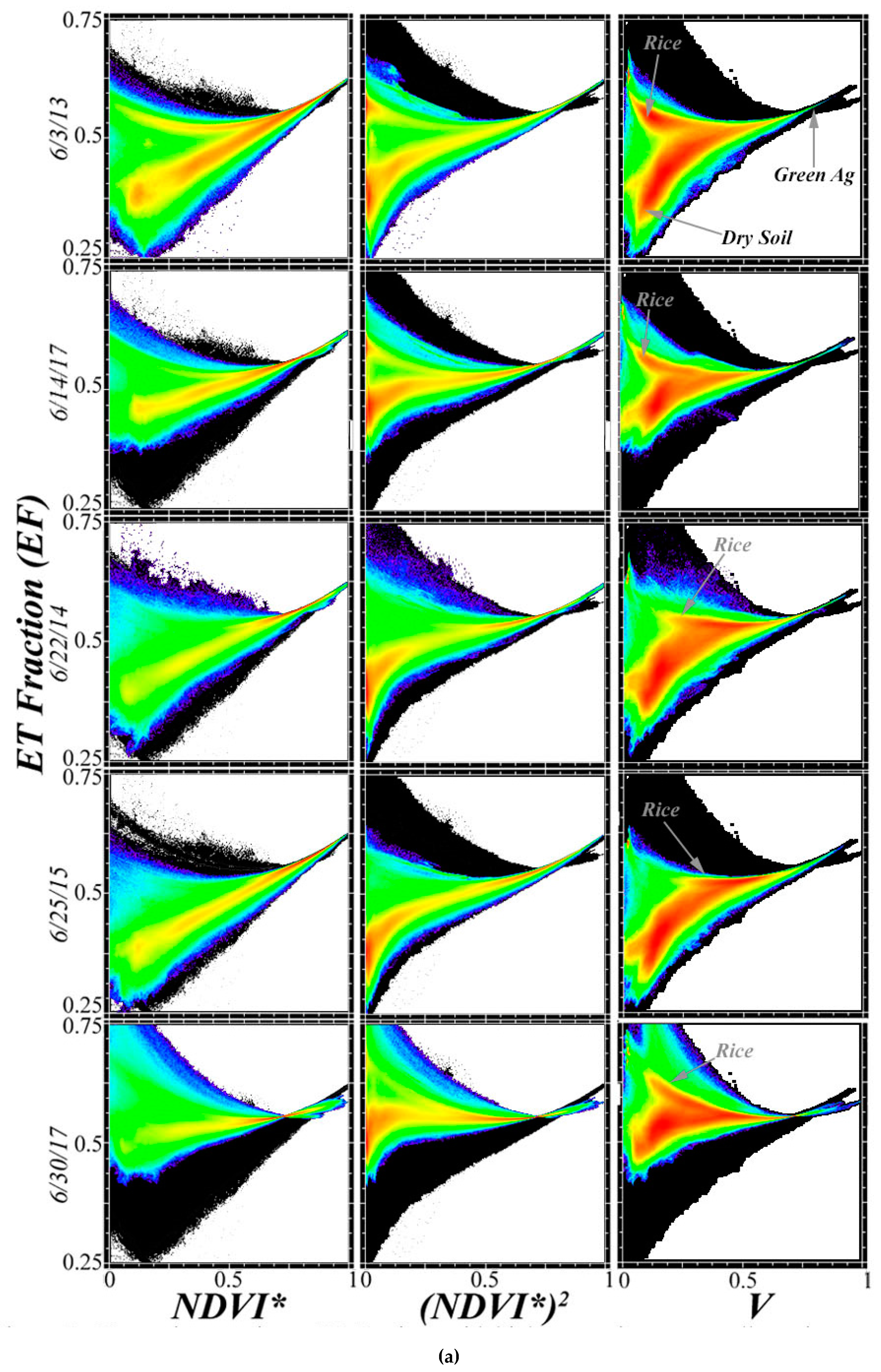
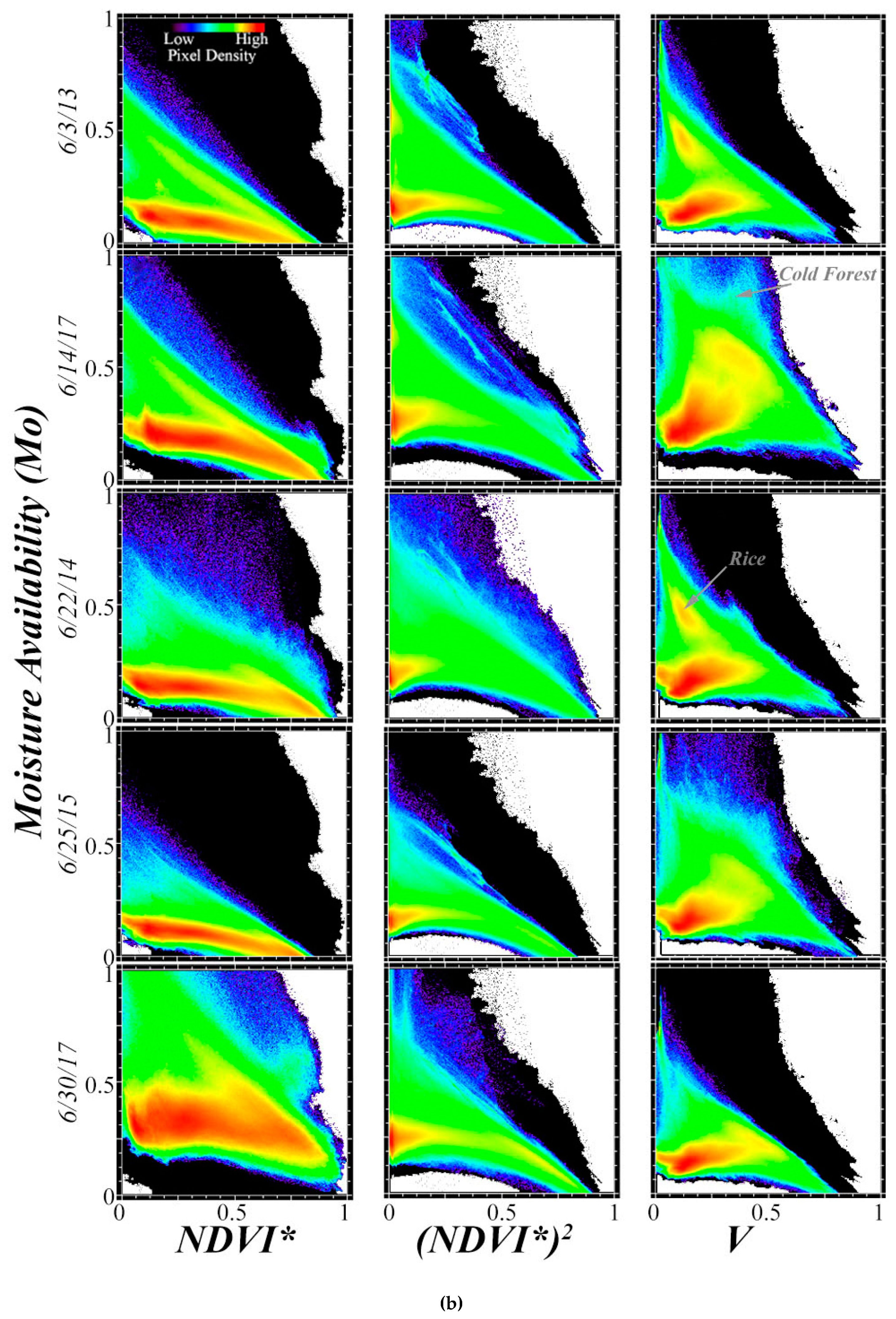
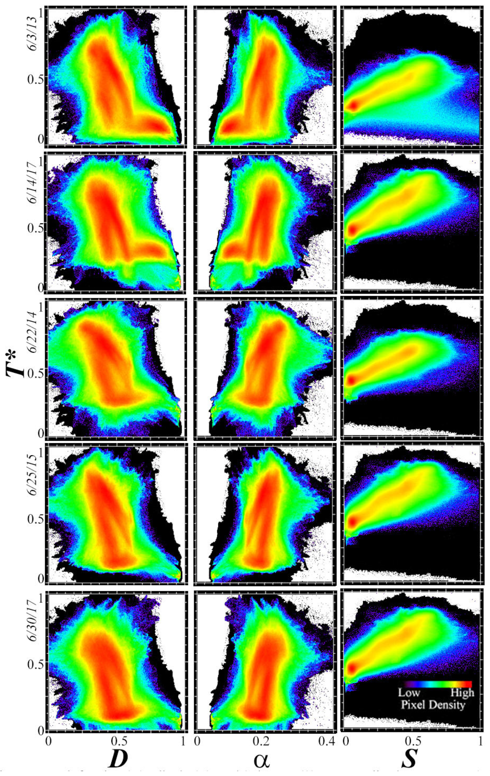
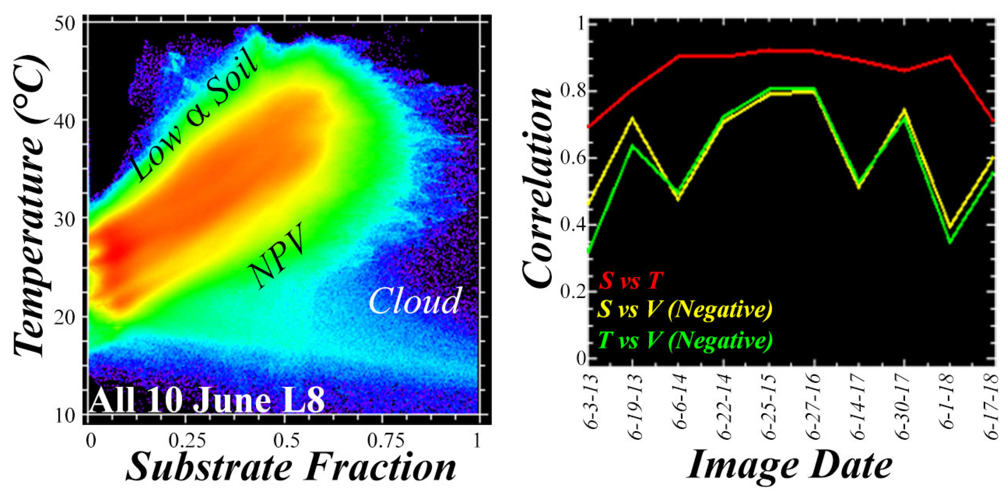
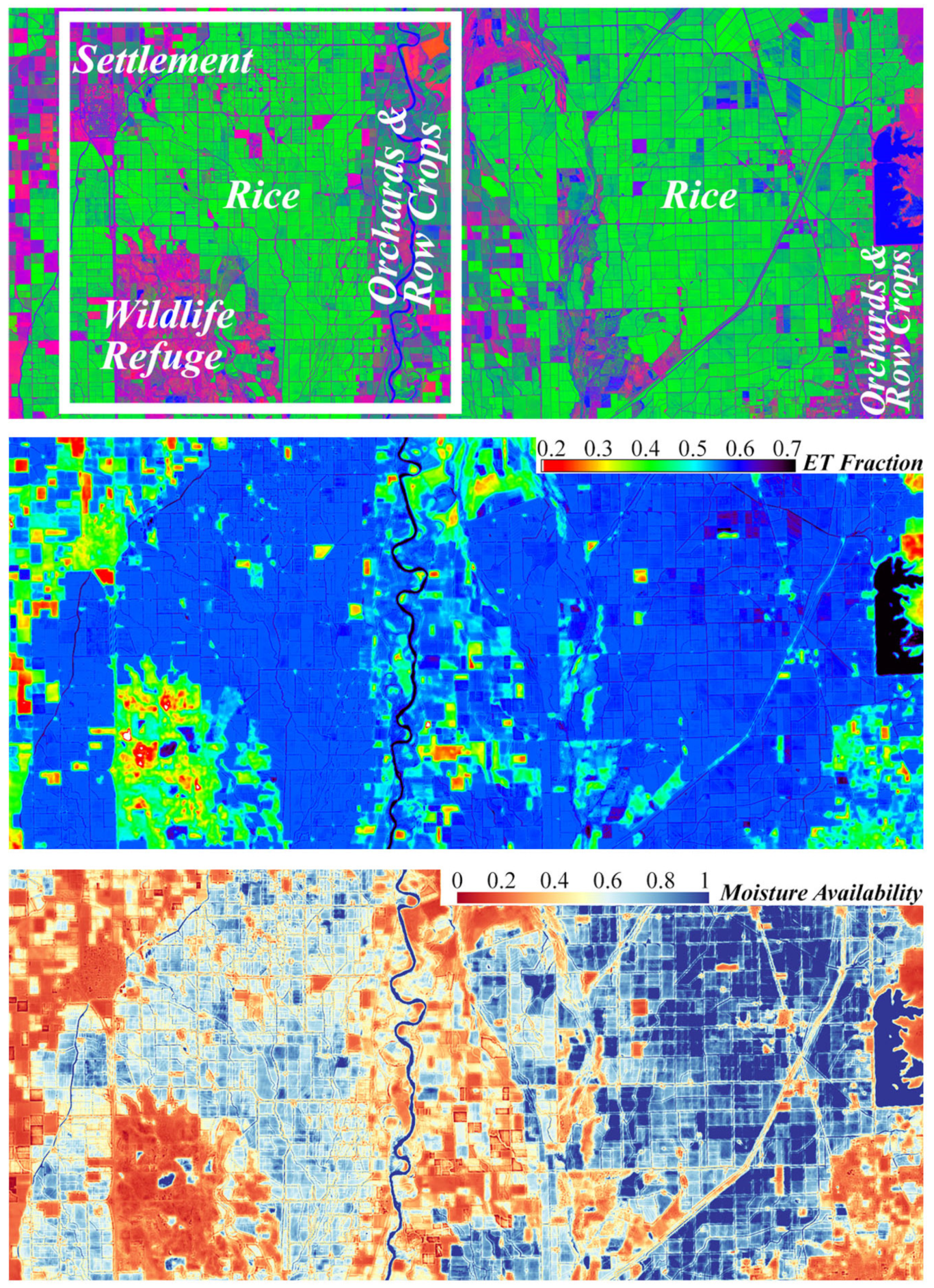
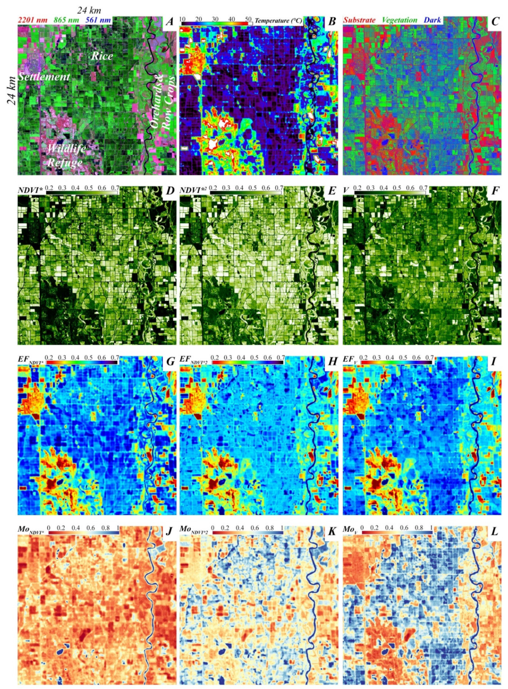
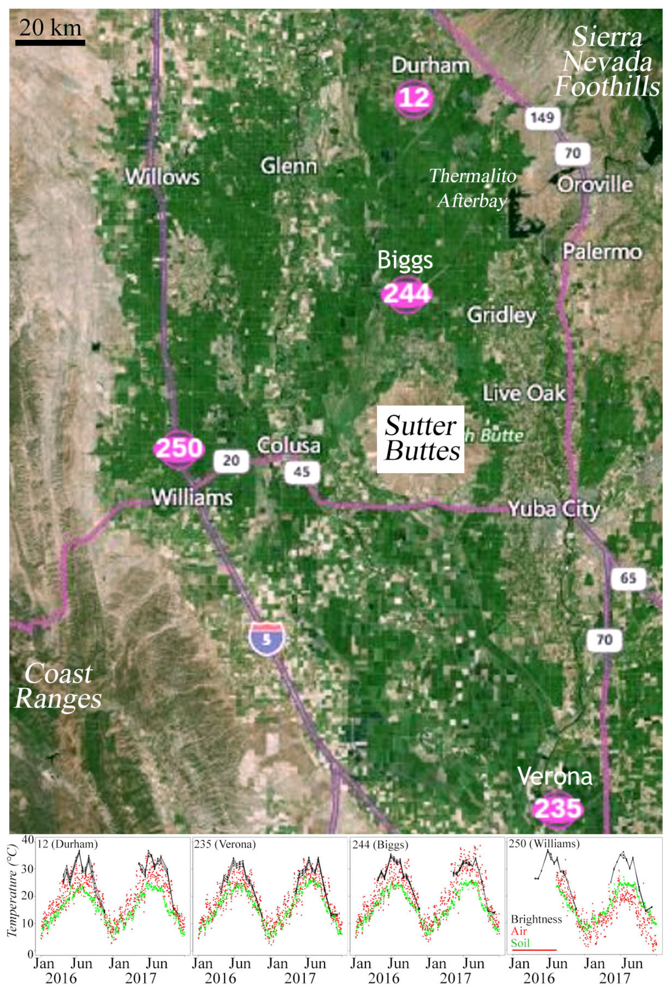
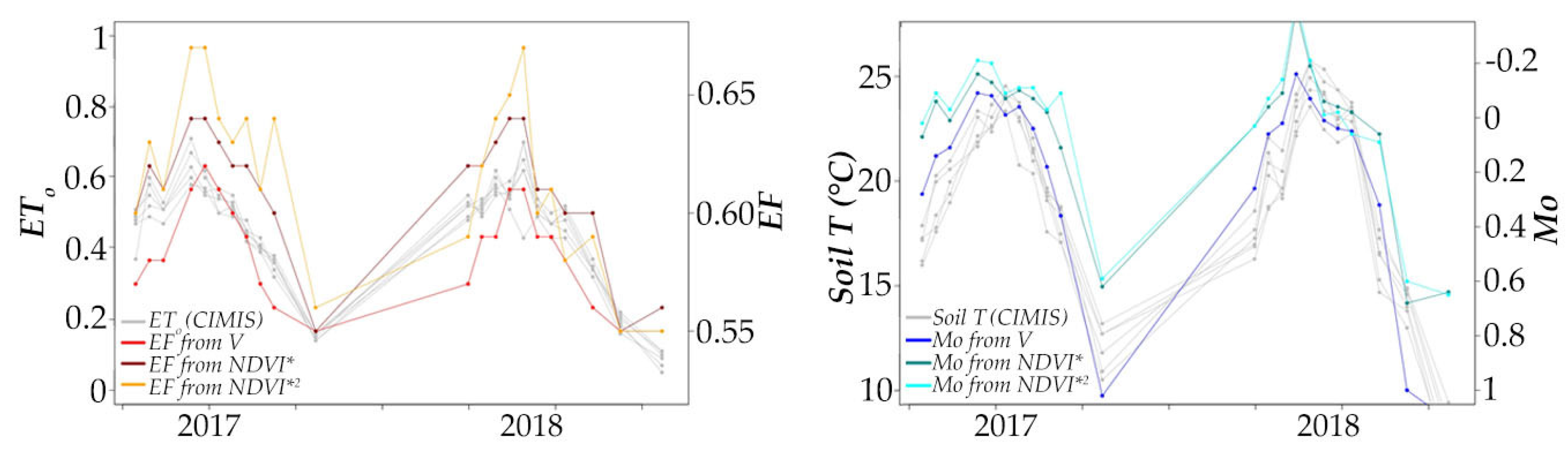
Table 1.
Generalized Triangle Method coefficients used to estimate EF and Mo. From Carlson (2007).
| r2 = 0.9993, RMSE = 0.017 | r2 = 0.9994, RMSE = 0.079 | ||||||||
|---|---|---|---|---|---|---|---|---|---|
| aij | j = 0 | j = 1 | j = 2 | j = 3 | aij | j = 0 | j = 1 | j = 2 | j = 3 |
| i = 0 | 0.8106 | −0.5967 | 0.4049 | −0.0740 | i = 0 | 2.058 | −1.644 | 0.850 | −0.313 |
| i = 1 | −0.8029 | 0.7357 | 0.0681 | 0.2302 | i = 1 | −6.490 | 1.112 | −3.420 | −0.062 |
| i = 2 | 0.4866 | 1.2403 | −0.9489 | −0.8676 | i = 2 | 7.618 | 3.494 | 10.869 | 4.831 |
| i = 3 | −0.3702 | −1.3943 | −0.7359 | 0.3860 | i = 3 | −3.190 | −3.871 | −6.974 | −16.902 |
© 2018 by the authors. Licensee MDPI, Basel, Switzerland. This article is an open access article distributed under the terms and conditions of the Creative Commons Attribution (CC BY) license (http://creativecommons.org/licenses/by/4.0/).
Share and Cite
MDPI and ACS Style
Sousa, D.; Small, C. Spectral Mixture Analysis as a Unified Framework for the Remote Sensing of Evapotranspiration. Remote Sens. 2018, 10, 1961. https://0-doi-org.brum.beds.ac.uk/10.3390/rs10121961
AMA Style
Sousa D, Small C. Spectral Mixture Analysis as a Unified Framework for the Remote Sensing of Evapotranspiration. Remote Sensing. 2018; 10(12):1961. https://0-doi-org.brum.beds.ac.uk/10.3390/rs10121961
Chicago/Turabian StyleSousa, Daniel, and Christopher Small. 2018. "Spectral Mixture Analysis as a Unified Framework for the Remote Sensing of Evapotranspiration" Remote Sensing 10, no. 12: 1961. https://0-doi-org.brum.beds.ac.uk/10.3390/rs10121961
Note that from the first issue of 2016, this journal uses article numbers instead of page numbers. See further details here.