Analysis of Mining Waste Dump Site Stability Based on Multiple Remote Sensing Technologies

Abstract
:
1. Introduction
2. Study Area and Dataset
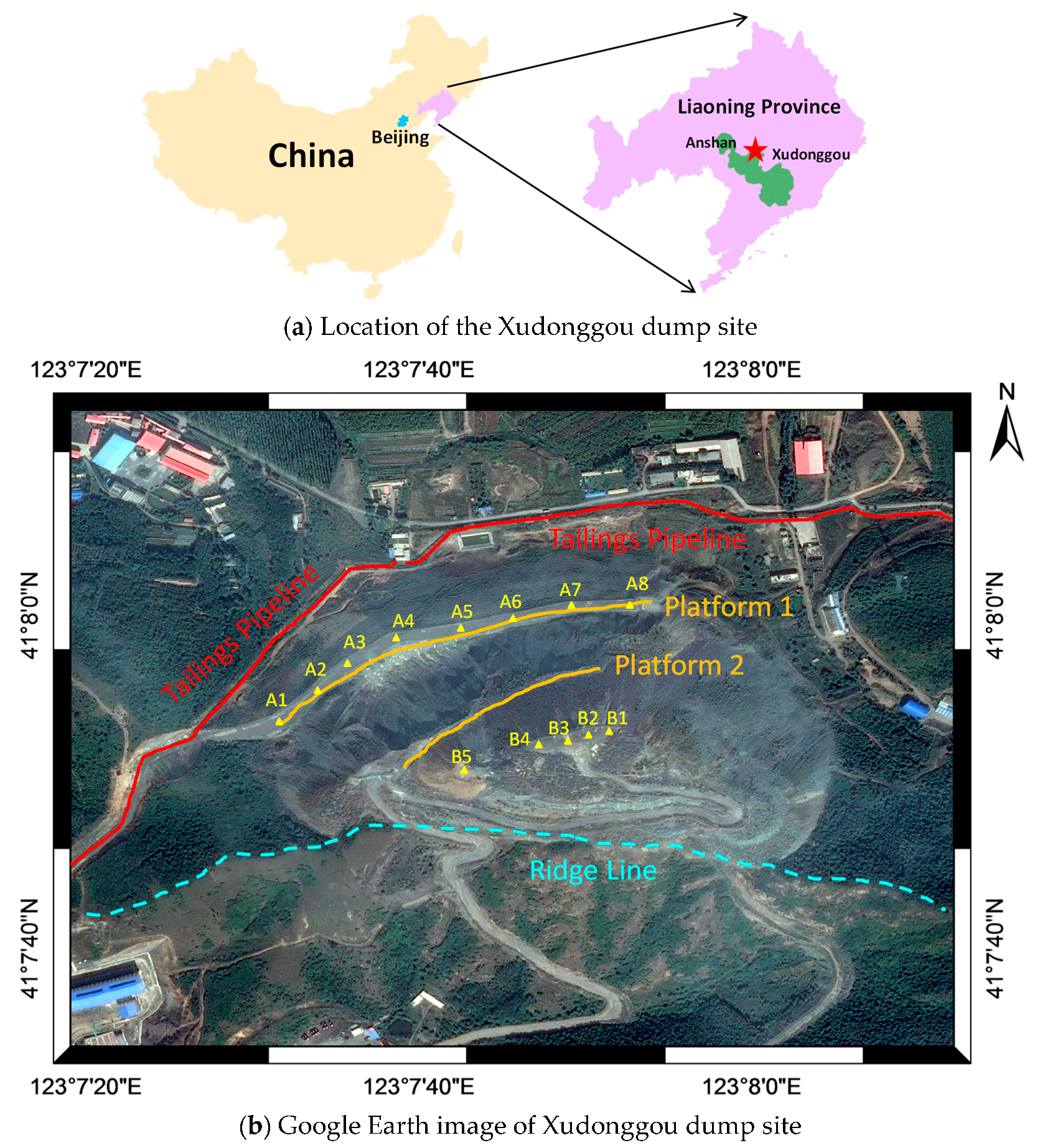
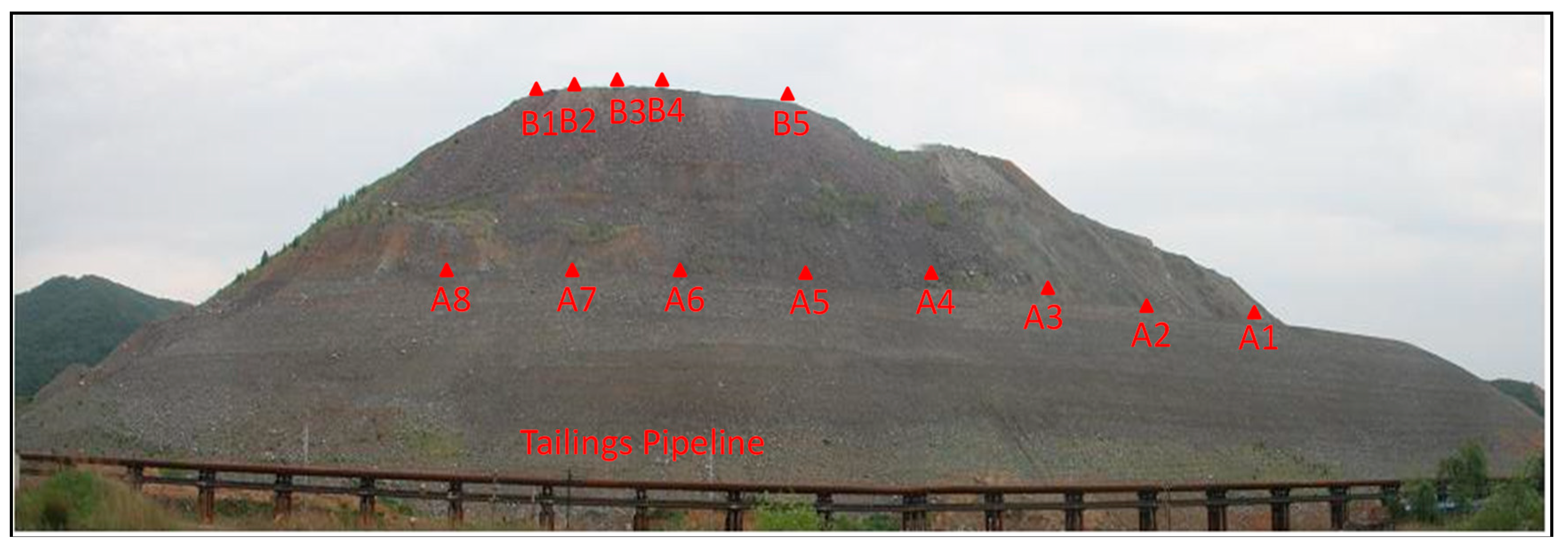
2.1. Study Area
2.2. Dataset
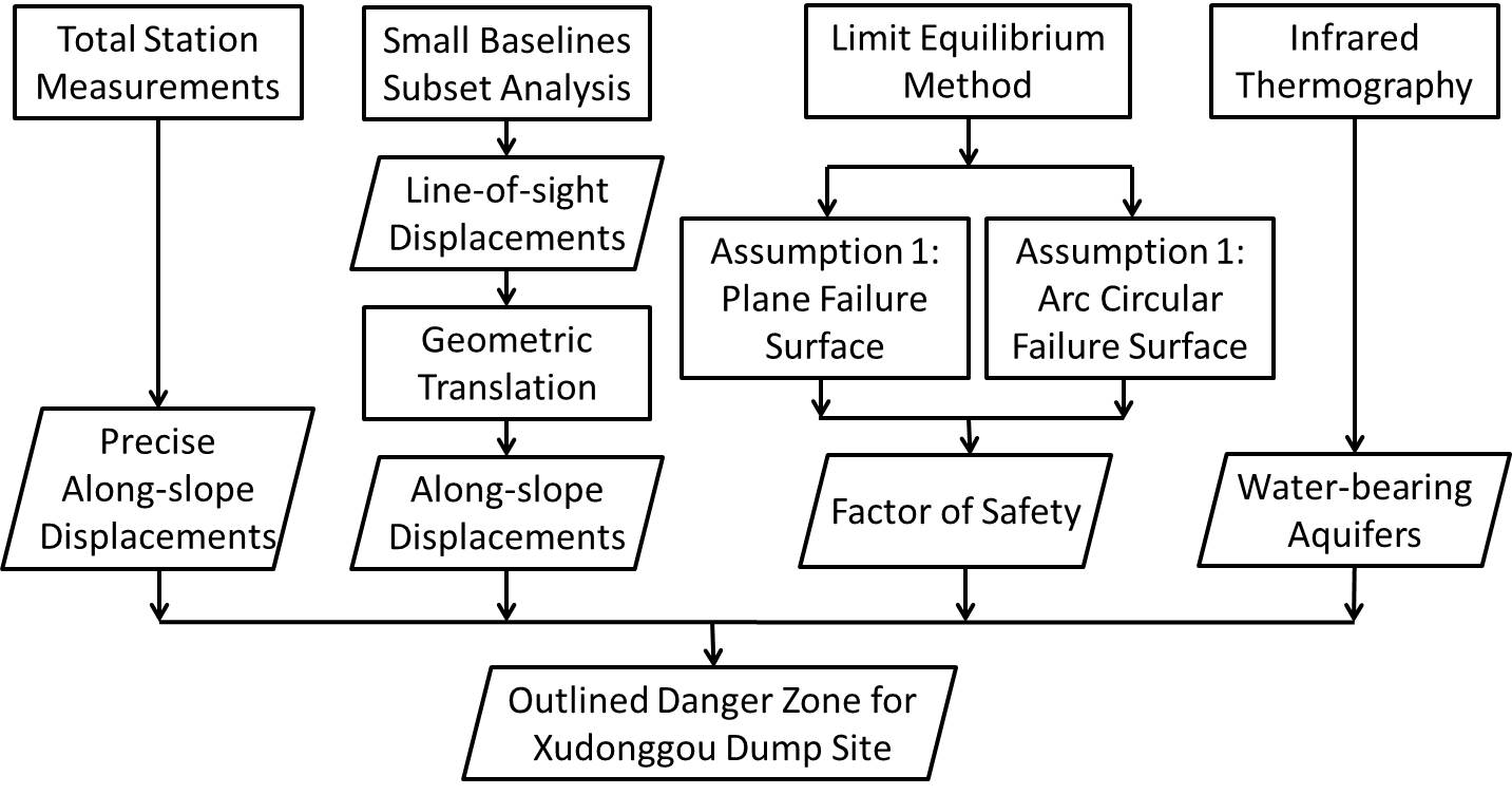
3. Methodology
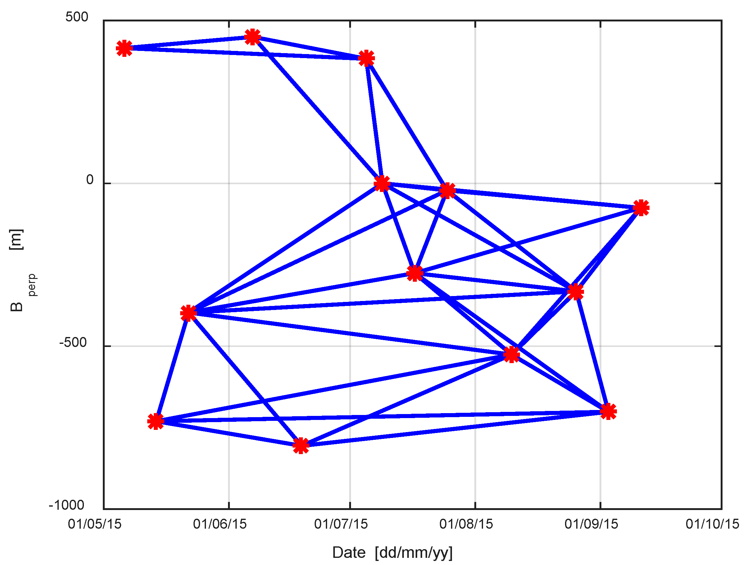
3.1. Small Baseline Subset Analysis
3.2. Infrared Thermography
3.3. Limit Equilibrium Method
4. Discussion of Experimental Results
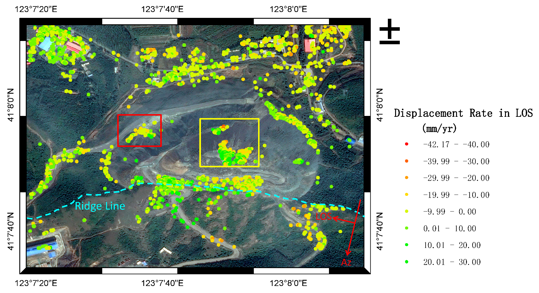
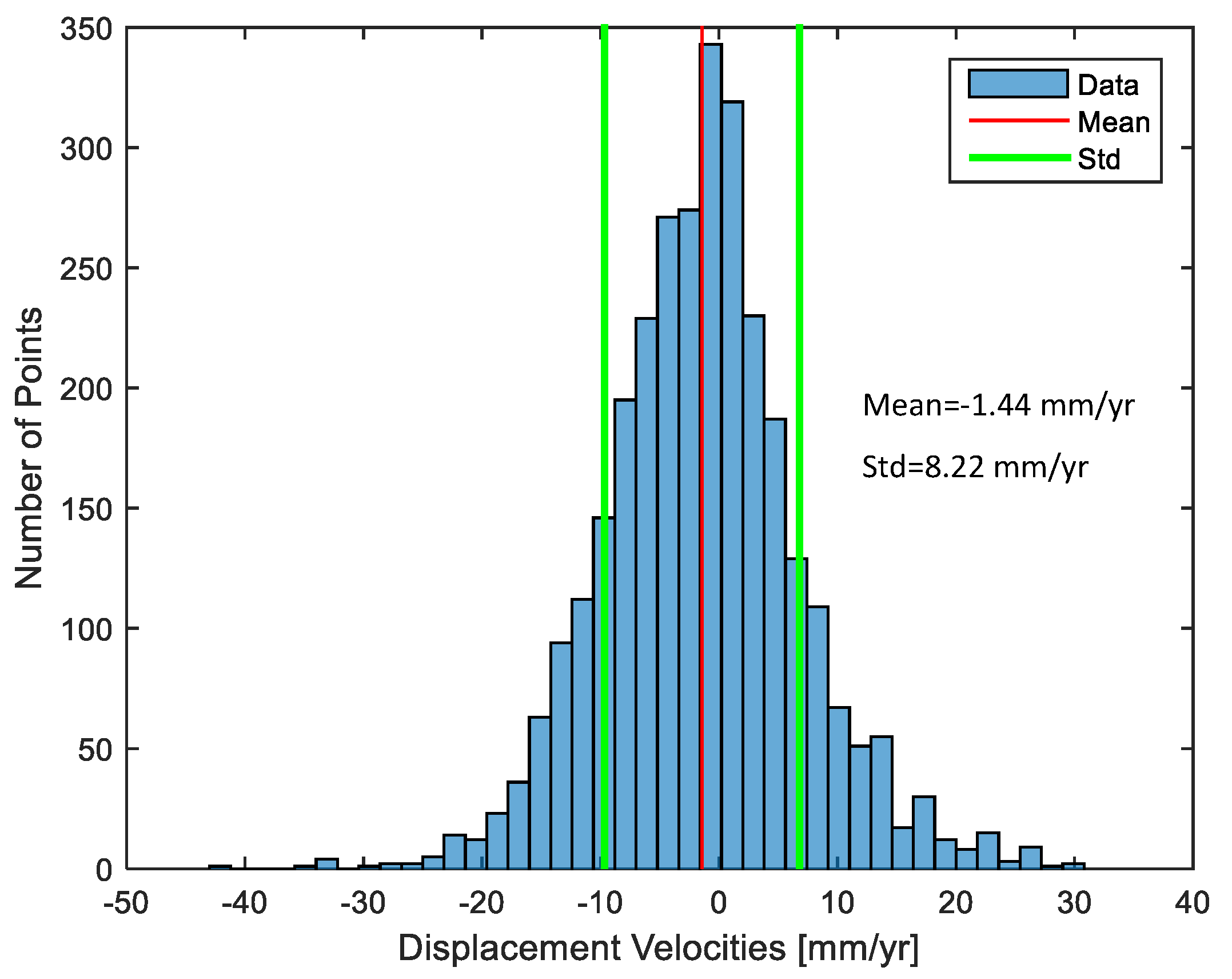
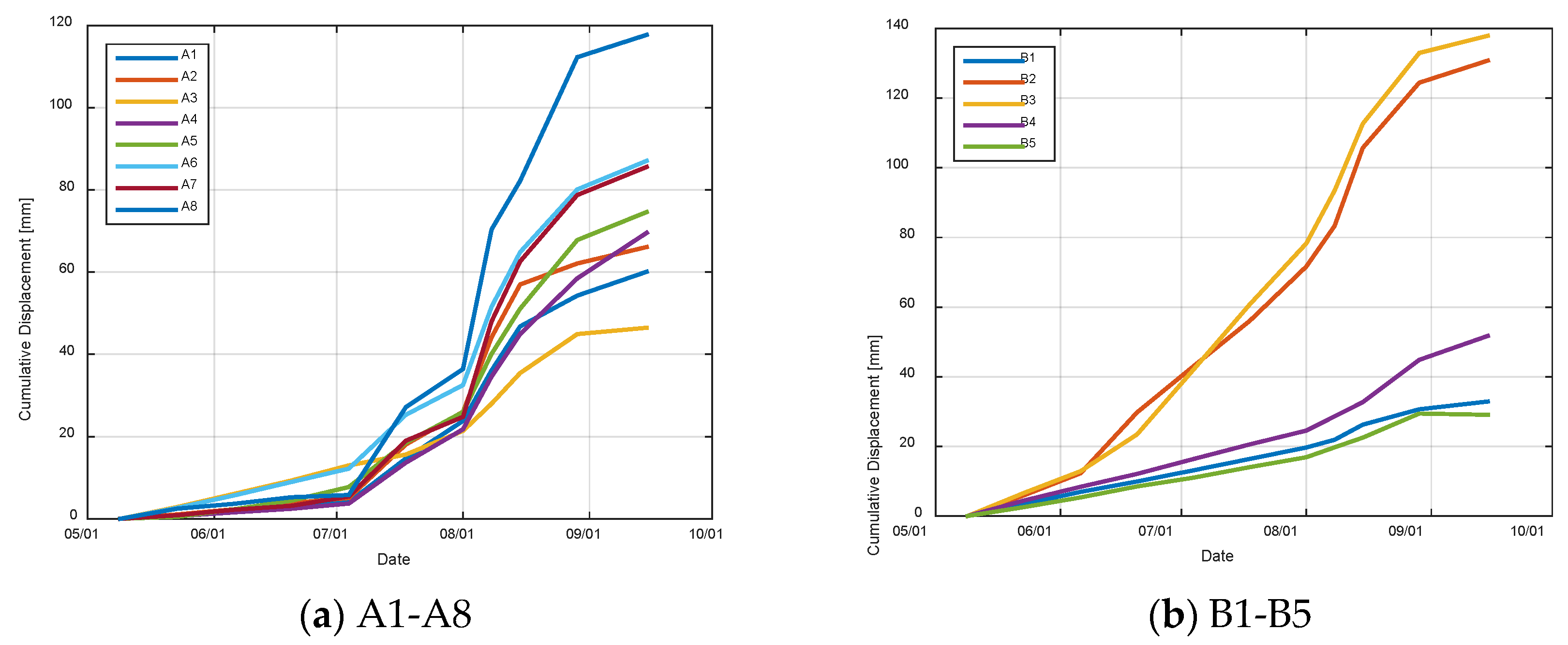
4.1. SBAS Results
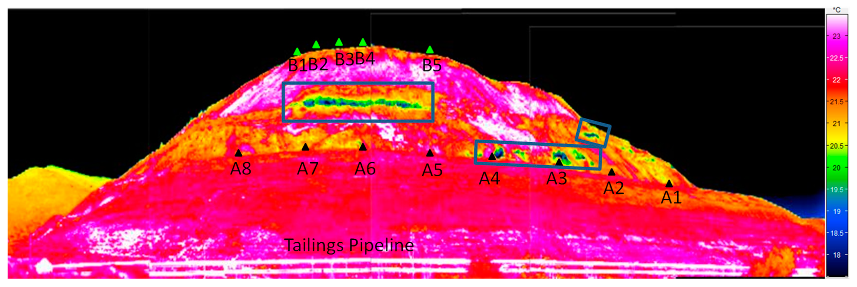
4.2. IRT Results
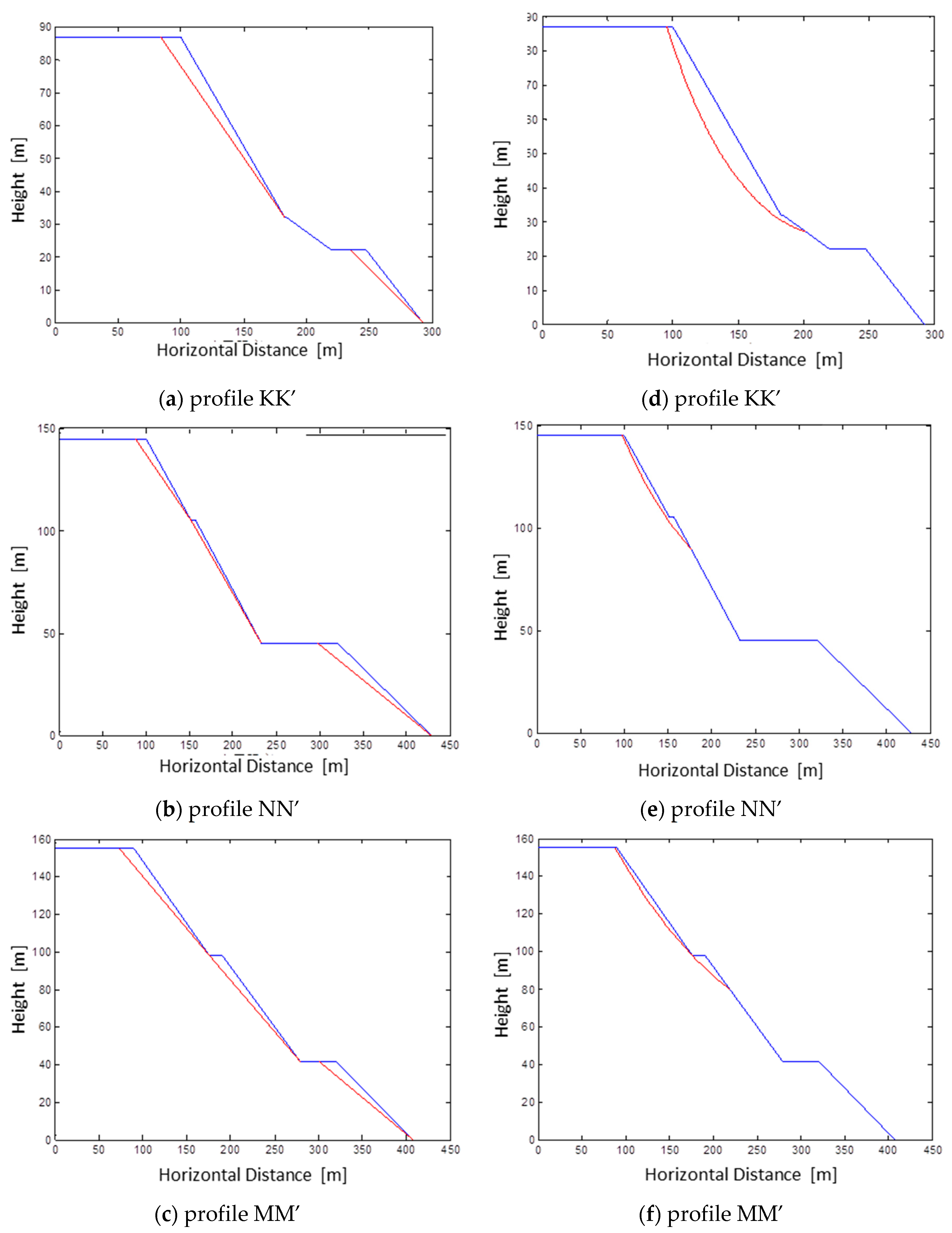
4.3. Numerical Simulation Based on the LE Method
5. Conclusions
Author Contributions
Funding
Acknowledgments
Conflicts of Interest
References
- Cho, Y.C.; Song, Y.S. Deformation measurements and a stability analysis of the slope at a coal mine waste dump. Ecol. Eng. 2014, 68, 189–199. [Google Scholar] [CrossRef]
- Steiakakis, E.; Kavouridis, K.; Monopolis, D. Large scale failure of the external waste dump at the “South Field” lignite mine, Northern Greece. Eng. Geol. 2009, 104, 269–279. [Google Scholar] [CrossRef]
- Zebker, H.A.; Goldstein, R.M. Topographic mapping from Interferometric Synthetic Aperture Radar observations. J. Geophys. Res. 1986, 91, 4993–4999. [Google Scholar] [CrossRef]
- Gabriel, A.K.; Goldstein, R.M.; Zebker, H.A. Mapping small elevation changes over large areas: Differential radar interferometry. J. Geophys. Res. 1989, 94, 9183–9191. [Google Scholar] [CrossRef]
- Ferretti, A.; Prati, C.; Rocca, F. Nonlinear subsidence rate estimation using permanent scatterers in differential SAR interferometry. IEEE Trans. Geosci. Remote Sens. 2000, 38, 2202–2212. [Google Scholar] [CrossRef]
- Ferretti, A.; Prati, C.; Rocca, F. Permanent scatterers in SAR interferometry. IEEE Trans. Geosci. Remote Sens. 2001, 39, 8–20. [Google Scholar] [CrossRef] [Green Version]
- Berardino, P.; Fornaro, G.; Lanari, R.; Sansosti, E. A new algorithm for surface deformation monitoring based on small baseline differential SAR interferograms. IEEE Trans. Geosci. Remote Sens. 2002, 40, 2375–2383. [Google Scholar] [CrossRef]
- Lanari, R.; Mora, O.; Manunta, M.; Mallorqui, J.J.; Berardino, P.; Sansosti, E. A small-baseline approach for investigating deformations on full-resolution differential SAR interferograms. IEEE Trans. Geosci. Remote Sens. 2004, 42, 1377–1386. [Google Scholar] [CrossRef]
- Mora, O.; Mallorqui, J.J.; Broquetas, A. Linear and nonlinear terrain deformation maps from a reduced set of interferometric SAR images. IEEE Trans. Geosci. Remote Sens. 2003, 41, 2243–2253. [Google Scholar] [CrossRef]
- Werner, C.; Wegmüller, U.; Strozzi, T.; Wiesmann, A. Interferometric point target analysis for deformation mapping. In Proceedings of the IEEE International Geoscience and Remote Sensing Symposium (IGARSS 2003), Toulouse, France, 21–25 July 2003; Volume 7, pp. 4362–4364. [Google Scholar]
- Kampes, B.M.; Hanssen, R.F. Ambiguity resolution for permanent scatterer interferometry. IEEE Trans. Geosci. Remote Sens. 2004, 42, 2446–2453. [Google Scholar] [CrossRef] [Green Version]
- Hooper, A. A multi-temporal InSAR method incorporating both persistent scatterer and small baseline approaches. Geophys. Res. Lett. 2008, 35, L16302. [Google Scholar] [CrossRef]
- Hooper, A.; Segall, P.; Zebker, H. Persistent scatterer Interferometric Synthetic Aperture Radar for crustal deformation analysis, with application to VolcanAlcedo, Galapagos. J. Geophys. Res. 2007, 112, B07407. [Google Scholar] [CrossRef]
- Zhang, L.; Ding, X.L.; Lu, Z. Ground settlement monitoring based on temporarily coherent points between two SAR acquisitions. ISPRS J. Photogramm. Remote Sens. 2011, 66, 146–152. [Google Scholar] [CrossRef]
- Zhang, L.; Ding, X.L.; Lu, Z. Modeling PSInSAR time series without phase unwrapping. IEEE Trans. Geosci. Remote Sens. 2011, 49, 547–556. [Google Scholar] [CrossRef]
- Zhang, L.; Lu, Z.; Ding, X.L.; Jung, H.S.; Feng, G.C.; Lee, C.W. Mapping ground surface deformation using temporarily coherent point SAR interferometry: Application to Los Angeles Basin. Remote Sens. Environ. 2012, 117, 429–439. [Google Scholar] [CrossRef]
- Hu, J.; Li, Z.W.; Ding, X.L.; Zhu, J.J.; Zhang, L.; Sun, Q. Resolving three-dimensional surface displacements from InSAR measurements: A review. Earth-Sci. Rev. 2014, 133, 1–17. [Google Scholar] [CrossRef]
- Gray, L. Using multiple RADARSAT InSAR pairs to estimate a full three-dimensional solution for glacial ice movement. Geophys. Res. Lett. 2011, 38, L05502. [Google Scholar] [CrossRef]
- Rocca, F. 3D motion recovery from multi-angle and/or left right interferometry. In Proceedings of the Third International Workshop on ERS SAR, Frascati, Italy, 1–5 December 2003. [Google Scholar]
- Wright, T.J.; Parsons, B.E.; Lu, Z. Toward mapping surface deformation in three dimensions using InSAR. Geophys. Res. Lett. 2004, 31, L01607. [Google Scholar] [CrossRef]
- Michel, R.; Avouac, J.P.; Taboury, J. Measuring ground displacements from SAR amplitude images: Application to the Landers earthquake. Geophys. Res. Lett. 1999, 26, 875–878. [Google Scholar] [CrossRef]
- Michel, R.; Avouac, J.P.; Taboury, J. Measuring near field coseismic displacements from SAR images: Application to the Landers earthquake. Geophys. Res. Lett. 1999, 26, 3017–3020. [Google Scholar] [CrossRef]
- Rott, H.; Stuefer, M.; Siegel, A.; Skvarca, P.; Eckstaller, A. Mass fluxes and dynamics of Moreno Glacier, Southern Patagonia Icefield. Geophys. Res. Lett. 1998, 25, 1407–1410. [Google Scholar] [CrossRef] [Green Version]
- Gray, A.L.; Short, N.; Mattar, K.E.; Jezek, K.C. Velocities and flux of the Filchner ice shelf and its tributaries determined from speckle tracking interferometry. Can. J. Remote Sens. 2001, 27, 193–206. [Google Scholar] [CrossRef]
- Simons, M.; Rosen, P.A. Interferometric Synthetic Aperture Radar geodesy. Treatise Geophys. 2007, 3, 391–446. [Google Scholar]
- Bechor, N.B.D.; Zebker, H.A. Measuring two-dimensional movements using a single InSAR pair. Geophys. Res. Lett. 2006, 33. [Google Scholar] [CrossRef] [Green Version]
- Jung, H.S.; Won, J.S.; Kim, S.W. An improvement of the performance of multiple-aperture SAR interferometry (MAI). IEEE Trans. Geosci. Remote Sens. 2009, 47, 2859–2869. [Google Scholar] [CrossRef]
- Rosi, A.; Agostini, A.; Tofani, V.; Casagli, N. A Procedure to map subsidence at the regional scale using the persistent scatterer interferometry (PSI) technique. Remote Sens. 2014, 6, 10510–10522. [Google Scholar] [CrossRef]
- Rosi, A.; Tofani, V.; Agostini, A.; Tanteri, L.; Tacconi Stefanelli, C.; Catani, F.; Casagli, N. Subsidence mapping at regional scale using persistent scatters interferometry (PSI): The case of Tuscany region (Italy). Int. J. Appl. Earth Obs. Geoinf. 2016, 52, 328–337. [Google Scholar] [CrossRef]
- Zhang, L.; Wu, J.C.; Ge, L.L.; Ding, X.L.; Chen, Y.L. Determining fault slip distribution of the Chi-Chi Taiwan earthquake with GPS and InSAR data using triangular dislocation elements. J. Geodyn. 2008, 45, 163–168. [Google Scholar] [CrossRef]
- Catalao, J.; Nico, G.; Hanssen, R.; Catita, C. Merging GPS and atmospherically corrected InSAR data to map 3-D terrain displacement velocity. IEEE Trans. Geosci. Remote Sens. 2011, 49, 2354–2360. [Google Scholar] [CrossRef]
- Tong, X.; Sandwell, D.T.; Smith-Konter, B. High-resolution interseismic velocity data along the San Andreas Fault from GPS and InSAR. J. Geophys. Res. 2013, 118, 369–389. [Google Scholar] [CrossRef] [Green Version]
- Guglielmino, F.; Bignami, C.; Bonforte, A.; Briole, P.; Obrizzo, F.; Puglisi, G.; Stramondo, S.; Wegmüller, U. Analysis of satellite and in situ ground deformation data integrated by the SISTEM approach: The April 3, 2010 earthquake along the Pernicana fault (Mt. Etna—Italy) case study. Earth Planet. Sci. Lett. 2011, 312, 327–336. [Google Scholar] [CrossRef]
- Guglielmino, F.; Nunnari, G.; Puglisi, G.; Spata, A. Simultaneous and integrated strain tensor estimation from geodetic and satellite deformation measurements to obtain three-dimensional displacement maps. IEEE Trans. Geosci. Remote Sens. 2011, 49, 1815–1826. [Google Scholar] [CrossRef]
- Hu, J.; Li, Z.W.; Sun, Q.; Zhu, J.J.; Ding, X.L. Three-dimensional surface displacements from InSAR and GPS measurements with variance component estimation. IEEE Geosci. Remote Sens. Lett. 2012, 9, 754–758. [Google Scholar]
- Del Soldato, M.; Farolfi, G.; Rosi, A.; Raspini, F.; Casagli, N. Subsidence evolution of the Firenze-Prato-Pistoia plain (Central Italy) combining PSI and GNSS data. Remote Sens. 2018, 10, 1146. [Google Scholar] [CrossRef]
- Joughin, I.R.; Kwok, R.; Fahnestock, M.A. Interferometric estimation of three dimensional ice-flow using ascending and descending passes. IEEE Trans. Geosci. Remote Sens. 1998, 36, 25–37. [Google Scholar] [CrossRef]
- Mohr, J.J.; Reeh, N.; Madsen, S.N. Three-dimensional glacial flow and surface elevation measured with radar interferometry. Nature 1998, 391, 273–276. [Google Scholar] [CrossRef]
- Kumar, V.; Venkataramana, G.; Hogda, K.A. Glacier surface velocity estimation using SAR interferometry technique applying ascending and descending passes in Himalayas. Int. J. Appl. Earth Obs. Geoinf. 2011, 13, 545–551. [Google Scholar] [CrossRef]
- Gourmelen, N.; Kim, S.W.; Shepherd, A.; Park, J.W.; Sundal, A.V.; BjÖrnsson, H.; Pálsson, F. Ice velocity determined using conventional and multiple-aperture InSAR. Earth Planet. Sci. Lett. 2011, 307, 156–160. [Google Scholar] [CrossRef] [Green Version]
- ISO 14688-1:2002: Geotechnical Investigation and Testing—Identification and Classification of Soil—Part 1: Identification and Description; International Organization for Standardization (ISO): Geneva, Switzerland, 2002.
- Binet, S.; Jomard, H.; Lebourg, T.; Guglielmi, Y.; Tric, E.; Bertrand, C.; Mudry, J. Experimental analysis of groundwater flow through a landslide slip surface using natural and artificial water chemical tracers. Hydrol. Process. 2007, 3472, 3463–3472. [Google Scholar] [CrossRef]
- Ronchetti, F.; Borgatti, L.; Cervi, F.; Gorgoni, C.; Piccinini, L.; Vincenzi, V.; Corsini, A. Groundwater processes in a complex landslide, northern Apennines, Italy. Nat. Hazards Earth Syst. Sci. 2009, 9, 895–904. [Google Scholar] [CrossRef] [Green Version]
- Bagherzadeh-Khalkhali, A.; Mirghasemi, A.A. Numerical and experimental direct shear tests for coarse-grained soils. Particuology 2009, 7, 83–91. [Google Scholar] [CrossRef]
- Covello, F.; Battazza, F.; Coletta, A.; Lopinto, E.; Fiorentino, C.; Pietranera, L.; Valentini, G.; Zoffoli, S. COSMO-SkyMed an existing opportunity for observing the Earth. J. Geodyn. 2010, 49, 171–180. [Google Scholar] [CrossRef] [Green Version]
- Huber, M.; Gruber, A.; Wendleder, A.; Wessel, B.; Roth, A.; Schmitt, A. The Global TanDEM-X DEM: Production Status and First Validation Results. In Proceedings of the 2012 XXII ISPRS Congress International Archives of the Photogrammetry, Remote Sensing and Spatial Information Sciences, Melbourne, Australia, 25 August–1 September 2012; Volume XXXIX-B7, pp. 45–50. [Google Scholar]
- The TanDEM-X 90m Digital Elevation Model. Available online: https://geoservice.dlr.de/web/dataguide/tdm90/ (accessed on 31 October 2018).
- Shi, X.; Liao, M.; Li, M.; Zhang, L.; Cunningham, C. Wide-area landslide deformation mapping with multi-path ALOS PALSAR data stacks: A case study of three gorges area, China. Remote Sens. 2016, 8, 136. [Google Scholar] [CrossRef]
- Maldague, X. Theory and Practice of Infrared Technology for Nondestructive Testing; Wiley: New York, NY, USA, 2001. [Google Scholar]
- Modest, M.F. Radiative Heat Transfer; Academic Press: Waltham, MA, USA, 2013. [Google Scholar]
- Gade, R.; Moeslund, T.B. Thermal cameras and applications: A survey. Mach. Vis. Appl. 2014, 25, 245–262. [Google Scholar] [CrossRef]
- Lahiri, B.; Bagavathiappan, S.; Jayakumar, T.; Philip, J. Medical applications of infraredthermography: A review. Infrared Phys. Technol. 2012, 55, 221–235. [Google Scholar] [CrossRef]
- Balaras, C.; Argiriou, A. Infrared thermography for building diagnostics. Energy Build. 2002, 34, 171–183. [Google Scholar] [CrossRef]
- Ibarra-Castanedo, C.; Tarpani, J.R.; Maldague, X.P. Nondestructive testing with thermography. Eur. J. Phys. 2013, 34, S91. [Google Scholar] [CrossRef]
- Sugiura, R.; Noguchi, N.; Ishii, K. Correction of low-altitude thermal images applied to estimatingsoil water status. Biosyst. Eng. 2007, 96, 301–313. [Google Scholar] [CrossRef]
- Liebmann, F. Infrared Target Temperature Correction System and Method. U.S. Patent 7,661,876, 16 Febuary 2010. [Google Scholar]
- Usamentiaga, R.; Venegas, P.; Guerediaga, J.; Vega, L.; Molleda, J.; Bulnes, F. Infrared Thermography for Temperature Measurement and Non-Destructive Testing. Sensors 2014, 14, 12305–12348. [Google Scholar] [CrossRef] [Green Version]
- Dai, F.; Lee, C.; Ngai, Y. Landslide risk assessment and management: An overview. Eng. Geol. 2002, 64, 65–87. [Google Scholar] [CrossRef]
- Upadhyay, O.P.; Sharma, D.K.; Singh, D.P. Factors affecting stability of waste dumps in mines. Int. J. Surf. Min. Reclam. Environ. 1990, 4, 95–99. [Google Scholar] [CrossRef]
- Tschuchnigg, F.; Schweiger, H.F.; Sloan, S.W. Slope stabilityanalysis by means of finite element limit analysis and finiteelement strength reduction techniques. Part I: Numericalstudies considering non-associated plasticity. Comput. Geotech. 2015, 70, 169–177. [Google Scholar] [CrossRef]
- Fellenius, W. Calculation of the stability of earth dams. In Proceedings of the Second Congress on Large Dams, Washington, DC, USA, 7–12 September 1936; Volume 4, pp. 445–463. [Google Scholar]
- Bishop, A.W. The use of the slip circle in the stability analysis of slopes. Geotechnique 1955, 5, 7–17. [Google Scholar] [CrossRef]
- Jambu, N. Slope Stability Computations; Soil Mechanics and Foundation Engineering Report; Technical University of Norway: Trondheim, Norway, 1968. [Google Scholar]
- Spencer, E. A method of analysis of the stability of embankments assuming parallel inter slices forces. Geotechnique 1967, 17, 11–26. [Google Scholar] [CrossRef]
- Weather History of ANSHAN. Available online: https://lishi.tianqi.com/anshan/index.html (accessed on 21 June 2018).


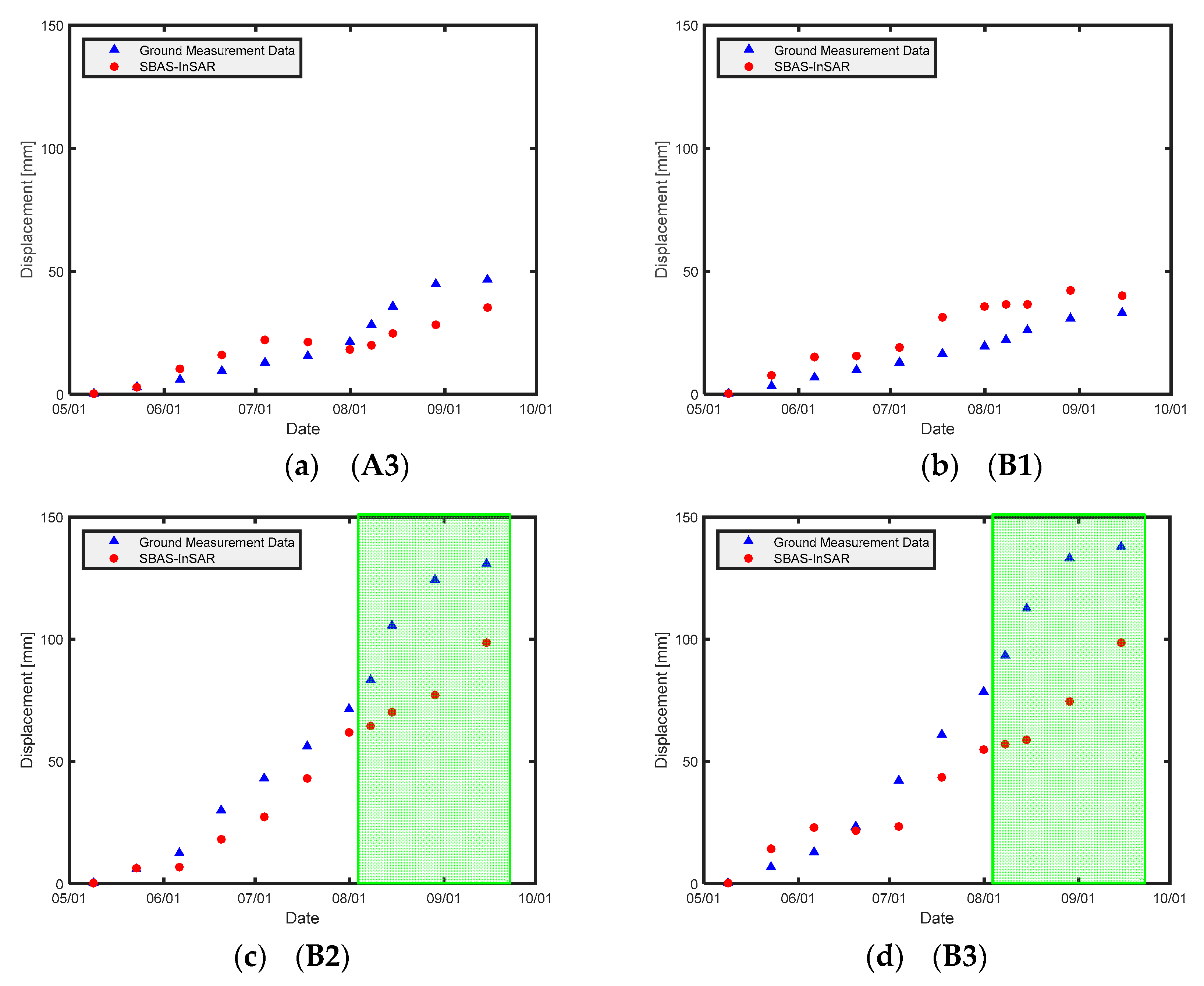
| Point ID | A3 | B1 | B2/B2_Corrected | B3/B3_Corrected |
|---|---|---|---|---|
| (mm) | −2.26 | 8.94 | −17.18/−7.89 | −20.99/−6.20 |
| RMSE (mm) | 8.09 | 4.79 | 14.54/5.91 | 22.66/12.46 |
| Profile Name | Slope 1 (Lower Part) | Slope 2 (Middle Part) | Slope 3 (Higher Part) | Total | ||||
|---|---|---|---|---|---|---|---|---|
| K2 | δ | K2 | Δ | K2 | δ | K2 | δ | |
| KK′ | 2.70 | 21 | 1.69 | 29 | - | - | 1.69 | 29 |
| NN′ | 2.71 | 19 | 1.51 | 36 | 1.56 | 32 | 1.08 | 36.5 |
| MM′ | 2.46 | 21 | 1.74 | 28 | 1.68 | 29 | 1.49 | 28 |
| Profile | KK′ | NN′ | MM′ |
|---|---|---|---|
| Most dangerous | 1.4115 | 1.0139 | 1.1673 |
| No. 2 dangerous | 1.4921 | 1.2104 | 1.3492 |
| Weak layer | - | 1.4078 | 1.5643 |
© 2018 by the authors. Licensee MDPI, Basel, Switzerland. This article is an open access article distributed under the terms and conditions of the Creative Commons Attribution (CC BY) license (http://creativecommons.org/licenses/by/4.0/).
Share and Cite
Wei, L.; Zhang, Y.; Zhao, Z.; Zhong, X.; Liu, S.; Mao, Y.; Li, J. Analysis of Mining Waste Dump Site Stability Based on Multiple Remote Sensing Technologies. Remote Sens. 2018, 10, 2025. https://0-doi-org.brum.beds.ac.uk/10.3390/rs10122025
Wei L, Zhang Y, Zhao Z, Zhong X, Liu S, Mao Y, Li J. Analysis of Mining Waste Dump Site Stability Based on Multiple Remote Sensing Technologies. Remote Sensing. 2018; 10(12):2025. https://0-doi-org.brum.beds.ac.uk/10.3390/rs10122025
Chicago/Turabian StyleWei, Lianhuan, Yun Zhang, Zhanguo Zhao, Xiaoyu Zhong, Shanjun Liu, Yachun Mao, and Jiayu Li. 2018. "Analysis of Mining Waste Dump Site Stability Based on Multiple Remote Sensing Technologies" Remote Sensing 10, no. 12: 2025. https://0-doi-org.brum.beds.ac.uk/10.3390/rs10122025