Modeling Solar Radiation in the Forest Using Remote Sensing Data: A Review of Approaches and Opportunities


1
Department of Geomatics and Spatial Planning, Faculty of Forestry, Warsaw University of Life Sciences, 02-787 Warsaw, Poland
2
Laboratory of Geomatics, Forest Research Institute, Sękocin Stary, 05-090 Raszyn, Poland
3
Department of Geoinformation, Institute of Urban Geography and Tourism, Faculty of Geographical Sciences, University of Lodz, 90-137 Lodz, Poland
*
Author to whom correspondence should be addressed.
Remote Sens. 2018, 10(5), 694; https://0-doi-org.brum.beds.ac.uk/10.3390/rs10050694
Submission received: 22 March 2018
/
Revised: 24 April 2018
/
Accepted: 26 April 2018
/
Published: 1 May 2018
(This article belongs to the Special Issue Solar Radiation, Modelling and Remote Sensing)
Abstract
:Solar radiation, the radiant energy from the sun, is a driving variable for numerous ecological, physiological, and other life-sustaining processes in the environment. Traditional methods to quantify solar radiation are done either directly (e.g., quantum sensors), or indirectly (e.g., hemispherical photography). This study, however, evaluates literature which utilized remote sensing (RS) technologies to estimate various forms of solar radiation or components, thereof under or within forest canopies. Based on the review, light detection and ranging (LiDAR) has, so far, been preferably used for modeling light under tree canopies. Laser system’s capability of generating 3D canopy structure at high spatial resolution makes it a reasonable choice as a source of spatial information about light condition in various parts of forest ecosystem. The majority of those using airborne laser system (ALS) commonly adopted the volumetric-pixel (voxel) method or the laser penetration index (LPI) for modeling the radiation, while terrestrial laser system (TLS) is preferred for canopy reconstruction and simulation. Furthermore, most of the studies focused only on global radiation, and very few on the diffuse fraction. It was also found out that most of these analyses were performed in the temperate zone, with a smaller number of studies made in tropical areas. Nonetheless, with the continuous advancement of technology and the RS datasets becoming more accessible and less expensive, these shortcomings and other difficulties of estimating the spatial variation of light in the forest are expected to diminish.

1. Introduction
The solar radiation in the form of light is a driving variable for many biological, ecological, physiological, and hydrological processes in the environment [1,2,3,4,5]. Aside from photosynthesis and transpiration, radiation in the forest also affects vegetation patterns [5,6], stand development [7], forest growth [5,8], and production efficiency [9,10]. By penetrating through the canopy, the influence of solar radiation can also be seen down to the forest floor, as it is also closely related to germination and understory growth [8,11], regeneration and succession [12,13,14], soil conditions [13,15,16], and even biodiversity [17,18]. It is, therefore, essential to have an understanding of the light condition if one wishes to study forest ecology [19].
Light intensity in the forest is mainly affected by canopy structure, site characteristics, atmospheric conditions and solar elevation [13,19,20,21,22,23]. These factors produce complex understory light patterns that express not only horizontal heterogeneity, but also the vertical variation at any given time [6].
Both solar elevation and atmospheric conditions are primarily dependent on the geographical location of the specified site. Thus, the discussions of these factors were deliberately excluded. The remaining factors: canopy structure and site characteristics are often represented and described with the use of remote sensing (RS) data [21,22,24,25]. Among others, canopy closure, canopy cover or canopy height are proxies of structural and geometrical information of leaves and branches, which are important variables characterizing light conditions inside the stand [6,9,19,26,27,28,29]. Such information carries critical parameters that can only be described effectively in a 3D space. In addition, site characteristics, such as micro relief, aspect, slope, and height above sea level, can be derived from an accurate high-resolution digital elevation model (DEM) acquired with the use of an active system, such as the light detection and ranging (LiDAR) [30,31]. Clearly, the remote sensing technology can be a very useful and important source of information for light condition inside the forest [32,33,34].
Existing comprehensive reviews on quantifying forest light environment have been published so far by Lieffers et al. [28], Comeau [35], and Promis [36]. The authors showed the nature and properties of the different instruments used, methods applied, the accuracies, as well as the associated costs. The use of handheld instruments, called ceptometers, and other quantum-equipped sensors as part of direct measurements, was widely mentioned, while hemispherical photography is considered the most common indirect way. Nonetheless, what was not considered in the scope of the three reviews, was the utilization of RS technology and other allied sciences.
Combined with field data, RS provides a handful of benefits, such as the generation of continuous spatial information with an effective cost on a wider scale. Modeling with the use of geographic information system (GIS), for example, can be used in lieu of field-recorded data for areas where field data is not available, or would be too expensive to record [37]. With this strategy, a continuous map of light conditions can be delivered as a final result.
While a passive optical sensor in two-dimensional format proved to be useful in various forestry applications, three-dimensional data may offer even more canopy details and a better understanding of the forest’s structure [38,39,40]. Aside from that, it overcomes some of the disadvantages of passive remote sensing, such as cloud-cover issues and vegetation index saturation problems [41]. A wide-ranging description of available airborne and satellite sensors and their capabilities, in general, could be referred to in the publications by Wang et al. [42], Brewer et al. [43] and, more recently, by Toth and Jozkow [44], with the latest discussions not only on sensors, but on platforms as well.
This paper, however, evaluates published articles that used or have at least a component of remote sensing in the context of solar radiation at forest stands in various scales. The aim of this study is to (i) synthesize the studies to determine how and what has been done with this state-of-the-art technology, and (ii) detect gaps in methodology or specific technology used to address improvements in the future. The first section of the review presents the physical concepts of solar radiation, and how it transmits through the canopy. The second section focuses on the different techniques and modeling approaches done by researchers on analyzing subcanopy solar radiation with the use of RS data. The next section discusses what we think are the critical issues that came out after synthesizing the articles, and selects papers that stand out and demonstrate novel approaches that only RS technology could offer. Lastly, conclusions and recommendations are laid down on how to improve future directions of similar studies.
2. Overview of Concepts
Scientists estimate that roughly 1368 watts m−2, averaged over the globe and over several years, illuminates the outermost atmosphere of the Earth [45]. This value is known as solar constant or the total solar irradiance (TSI), which is the maximum possible power that the sun can deliver to the Earth at the mean distance between them [23,46]. Only about ¼ of the TSI that is considered the incoming solar radiation, collectively called shortwave radiation, enters the top of Earth’s atmosphere [46]. Out of this proportion, approximately 20% and 30% is absorbed by the atmosphere and reflected back to space, respectively [1]. The remaining 50% penetrates the atmosphere, and is taken in by the land and the oceans [45]. Gibson [47] said that about half of the shortwave radiation is in the visible region (0.4–0.7 μm) of the electromagnetic spectrum, and the other half is mostly in the near-infrared (0.7 μm–100 μm). Ultraviolet radiation (0.01–0.4 μm) makes up only a little over 8% of the total [47]. The entire spectrum of the absorbed radiation drives photosynthesis, fuels evaporation, melts snow and ice, and warms the Earth [46].
Once the shortwave radiation touches the Earth’s surface, there are three forms of interactions that take place—absorption, transmission, and reflection [48]. Their proportions depend on the wavelength of the energy, and the material and condition of the feature [48]. According to Brown and Gillespie [49], a single layer of leaf will generally absorb 80% of incoming visible radiation, whilst reflecting 10% and transmitting the remaining 10%. Approximately 20% of infrared is absorbed, with 50% reflected and 30% transmitted. These interactions may be modified considering the heterogeneous spatiotemporal characteristics of canopy based on the type of leaf, arrangements, density, and the angle of incidence which determines the projected (“shadowed”) leaf area in the direction of the radiation [8,50,51].
Furthermore, in a subcanopy environment, the direct component of radiation is more heterogeneous than the diffused light. A predominantly direct-beam radiation that passes through openings in the forest canopy is called sunfleck [52]. The amount of sunfleck in the understory depends on different, often interacting factors: the coincidence of solar path with a canopy opening, the movement of clouds that obscure or reveal the sun, and the wind-induced movement of foliage and branches [53]. On the other hand, the penetration of the diffuse light is less variable, as it depends on the level of sky brightness, and the number, size, and spatial distribution of canopy openings, the canopy geometry, and the spatial distribution and optical characteristics of the forest biomass [54].
Generally, solar radiation below the canopy and on the forest floor has been expressed as transmittance, which depends on (1) the density and thickness of the vegetation layer, (2) the terrain, and (3) the position of the sun [36,55]. Comeau [35] defined transmittance as the ratio of solar radiation that reaches a sampling point within a forest to the incident radiation measured in the open or over the canopy at the same time. A widely accepted theory on light transmission in the forest is used by treating the canopy as a turbid medium [34,35]. This equation is called the Beer–Lambert–Bouguer law, or simply, Beer’s law [6,56]:
where: I = below-canopy light intensity
- = incident radiation at the canopy top
- k = extinction coefficient
- L = leaf area index (LAI)
The extinction coefficient which corresponds to an optical depth per unit leaf area [51] is determined by a number of factors, such as leaf angle distribution, canopy structure, and clumping level [57]. Depending on the type of vegetation, it usually varies between 0.3 and 0.6 [57,58,59]. For an assumed spherical leaf angle distribution, k is approximated as a function of the solar zenith angle θ [23,58]:
The LAI which represents a structure parameter in the vertical direction is defined as the total one-sided area of leaf tissue per unit ground surface area (m2 m−2) [51,57]. Nearly all vegetation and land-surface models include parameterizations of LAI, as it characterizes the canopy–atmosphere interface, where most of the energy fluxes exchange [57,60]. Estimation of the LAI can be derived from light transmission applying Beer’s law, where the fraction of light that is intercepted (T) changes exponentially as the layer of leaves increases [61]:
So, with a theoretical value of 0.5 for k, an LAI of 1, 3, 6, and 9 intercepts, respectively, 39, 78, 95, and 99% of the visible light [61].
In addition, Nyman et al. [55] describes another way to measure transmittance as a function of the path length (P), based on the earlier work of Seyednasrollah and Kumar [62]. In this approach, the density of the vegetation and the extinction coefficients are combined into a single parameter which describes the rate of absorption per unit path length. Path length of the direct beam is computed as the ratio of canopy height and cosine of solar zenith angle (Figure 1). The probability of attenuation of an incident radiation is directly proportional to the path length itself, leaf density (ratio of LAI and canopy height) and the leaf area facing the beam of light, or the leaf normal oriented in the light’s direction [63].
Solar radiation energy is often measured as an energy flux density (watts per square meter), and is appropriate for energy balance studies because watt is a unit of power [23,64]. But for studies of light interception in relation to plant’s health and growth, the photon density is better suited because the rate of photosynthesis depends on the number of photons received, rather than photon energy [23]. The specific range of 400 to 700 nm wavelength is where photosynthesis is active, and so it is called the photosynthetically active radiation or PAR region [64,65]. Owing to its similarity to spectral range, PAR is often used synonymously with visible light [28,66]. Energy in the PAR region is referred to as photosynthetic photon flux density (PPFD), with units in μmol m−2 s−1 [65].
3. Modelling Approaches Using RS Technology
Based on the selected scientific literatures, a schematic diagram (Figure 2) was created to illustrate how the authors made use of RS technology in building their models. Airborne laser scanning (ALS) and terrestrial laser scanning (TLS) are the two commonly used systems, while additional information was taken from optical images either from satellites or UAV-based digital cameras. Point clouds from either ALS or TLS were processed and transformed into voxels, where transmission model was applied. Most of the voxel modeling relied on Beer–Lambert–Bouguer law, where attenuation of sunlight is calculated as a function of vegetation structure. Generation of LiDAR metrics, such as canopy height or canopy density, was also observed, then used as inputs for further analysis. Others used it in ray-tracing model or as a substitute to LAI, particularly in Equation (1). For simulation of light regime, reconstruction of the canopy was performed especially from the TLS dataset. Letters (a) and (b) of Figure 2 illustrate how laser pulses best represent the direct beam of sunlight hitting various parts of the canopy, as well as the ground. Detailed discussions on how these techniques were executed are given in the subsequent section.
3.1. Physical Models and Techniques
Most of the authors depended on the capability of laser technology where 3D generation of the data is possible. It is probably one of the major advantages of LiDAR over other sensors. The usage of voxel or volumetric pixel modeling is on top of the list where the structure of the canopy is represented by cubical volume elements that are either filled with elements of the vegetation, or not [12,67,68]. The biophysical and structural property of a forest canopy can be derived from LiDAR technique with high detail [16,67].
Another technique of 3D model generation is the explicit geometric reconstruction of the canopy itself as “seen” by the sensor, and then simulation of the radiation regime within it. TLS has been tested successfully as a tool to reconstruct canopy structures, tree trunk, and diameter at breast height (DBH) to estimate LAI, stem volume, and aboveground biomass [38,39,69,70,71]. Van Leeuwen et al. [34] used this kind of technique with good results, utilizing the Echidna Validation Instrument (EVI). EVI is a ground-based laser waveform-recording, multiview angle-scanning LiDAR system designed to capture the complete upper hemisphere, and down to a zenith angle of just under 130° [72]. EVI was demonstrated to retrieve forest stand structural parameters, such as DBH, stand height, stem density, LAI, and stand foliage profile, with impressive accuracy [73]. The data used by Van Leeuwen et al. [34] for stem and canopy reconstruction pipeline was discrete, but the point clouds were derived from full waveform data. Single and last returns were used for creating virtual geometric models of the forest plots. These returns were obtained from the full waveform information using methods described by Yang et al. [71]. Jupp et al. [72] were able to process EVI data to generate canopy gap probabilities at different zenith ring ranges to infer radiation transmission. The canopy gap probability is equivalent to the probability that the ground surface is directly visible from airborne and spaceborne remote sensing platforms [74]. Both Van Leeuwen et al. [34] and Yang et al. [75] found strong relationships between the transmission properties of their respective radiation models and EVI-derived gap probabilities.
Other light transmission models, that are not in the reviewed articles but worth mentioning, are LITE (Light Interception and Transmittance Estimator) [76], SLIM (Spot Light Interception Model) [77], and DART (Discrete Anisotropic Radiative Transfer) [78]. The first two models are separate executable programs that provide a flexible association of utilities for entering light data from several sources and for outputting 3D estimates of leaf area and both instantaneous and seasonal PPFD beneath tree canopies [77]. SLIM prepares data for entry into LITE, but SLIM is also a “stand-alone” utility designed to estimate leaf area index (LAI), gap fraction, and transmittance from hemispherical photographs or ceptometer data. LITE provides maps of LAI and PPFD across the study site, and provides information on the light regime at selected locations [79]. However, we believe that there has not been any attempt yet to integrate RS data to either of the models.
DART [78] is probably one of the most popular tools for simulating remote sensing images for conducting physical models [80,81]. Developed by the Center for the Study of the Biosphere from Space (CESBIO) laboratory in France, DART is a comprehensive physically-based 3D model for Earth–atmosphere radiation interaction, from visible to thermal infrared. It simulates measurements of passive and active satellite/plane sensors for urban and natural landscapes. These simulations are computed in any experimental (atmosphere, terrain, forest, date) and instrumental (spatial and spectral resolutions, viewing direction) configuration [78]. DART successfully simulated reflectance of forests at different spectral domains [82]. The model just recently introduced a method to simulate LiDAR signals, and showed potential for forestry applications [83], but we have not found any actual research applying the model to a specific site.
Whether it is a simple equation-type or computer-based light model, various inputs are needed, which LiDAR metrics can provide. At least four of the articles [16,84,85,86] generated LiDAR-derived canopy or tree metrics before executing their models. Some of these metrics are canopy height and canopy density, essential for voxel modeling. As emphasized by Mucke and Hollaus [13], knowledge about the canopy architecture, meaning the spatial composition of trees or bushes, and the arrangement of their branches and leaves or needles, is of critical importance for the modeling of light transmission, and no other technique, except LiDAR, is well-suited for the derivation of canopy’s geometric information. Moreover, there is a different kind of LiDAR format, called full waveform, which is designed to digitize and record the entire backscattered signal of each emitted laser pulse [87]. Full-waveform data is rich in information, and is particularly useful for mapping within a canopy structure [88]. Unlike the basic metrics from the more popular discrete point clouds, however, this type of system is rarely used, due to acquisition costs, data storage limitations, and the lack of physically-based processing methods for their interpretation [88,89].
Laser beams could act as sunrays (a and b of Figure 2), which are either intercepted by leaves and branches, or penetrate through the holes. The latter is analogous to what a laser penetration index (LPI) does, which, according to Barilotti et al. [90], explains the ratio of the points that reach the ground over the total points in an area. In contrast, Kwak and Lee [91] exploited those point clouds intercepted by the crown, and called it the laser interception index (LII). LPI and LII were used separately to predict LAI ,and both produced high accuracy results [90,91]. For radiation studies, LPI was used by Yamamoto et al. [84], and successfully estimated the transmittance, even with low pulse density (e.g. 2.5 pulses m−2). They utilized a modified LPI to automatically and easily separate the laser pulses into those of canopy and below-canopy returns. The system was called Automated LiDAR Data Processing Procedure (ALPP) [92] and worked by integrating LiDAR Data Analysis System [93] and GRASS software. In ALPP, a top surface model was first created from the locations of treetops extracted from the LiDAR data within a plot. Then, the return pulses within the plot were converted to vertical distance (VD) from which the frequency distribution of 0.5 m class VD was statistically separated into canopy and below-canopy classes. Finally, linear regression between the LPI and diffuse transmittance taken from hemispherical photographs was performed. The highest coefficient of determination (R2 = 0.95) of the regression line was seen at 12.5 m radius LPI cylindrical plots. The accuracy of the methodology may be put to test upon applying to a different forest or a species-type other than cypress in Japan. Moreover, from a logical point of view, the analogy of LPI seemed to be more appropriate for direct component rather than the diffuse one. Musselman et al. [16] utilized LPI to infer solely the direct beam transmittance inside a conifer forest for various types of land surface modeling, such as melting snow. Interestingly, the most effective radius they discovered for LPI extraction, to estimate LAI, was 35 m; almost 3× that of the findings by Yamamoto et al. [84]. Although Musselman et al. [16] used a Beer’s type model specific to direct beam for LAI estimation, this may still be debatable, because like diffuse transmittance, they are both closely related.
Alexander et al. [21] used ALS as a proxy to a hemispherical camera by transforming point clouds into canopy cover and canopy closure. The former was made possible by generating Thiessen polygons from the ALS points, while the latter was done by plotting the same points in the polar coordinate system, with the azimuth angle as the angular coordinate, and the zenith angle as the radial coordinate. Moreover, these synthetic images mimicking hemispherical photos were correlated to the species classified according to Ellenberg values [94]. These values, ranging from 1 to 9, represent varying shade tolerance with 1 denoting species preferring deep shade, and 9 for species preferring full sunlight. It revealed that ALS-based canopy closure is a reasonable indicator of understory light availability, and has the advantage over field-based methods that it can be rapidly estimated for extensive areas.
A convenient way to generate spatial information is to have a working environment in a GIS platform. GIS software that comes with a solar radiation analysis package that could estimate irradiance at a watershed scale has been used by a number of researchers [22,95]. GIS solar models operate on digital terrain model (DTM) raster layers, allowing them to accurately estimate insolation reduction due to slope, aspect, and topographic shading across watersheds [96]. Both Solar Analyst from ESRI’s ArcGIS, and from that of Helios Environmental Modeling Institute, adapt the sky region technique used in hemispherical photos for use with raster grids [97]. On the other hand, the r.sun module of the GRASS software (see sample map in Figure 3) is a clear sky solar model designed to take topographic angles and shading into account [98].
3.2. Summary of the Studies
Table 1 summarizes the literature subjected for review. Each paper’s salient features, some of them unique, are described briefly.
The reviewed studies were generally classified based on the type of sensor the authors preferred to use, either as active or passive. The latter is a type of system that uses the sun as the source of electromagnetic radiation, while the former pertains to sensors that supply their own source of energy to illuminate features of interest [47,105]. Digital cameras on board UAVs and satellite optical imagery sensors are passive types, while radar and LiDAR technologies belong to active sensors. It was found out that the majority of the studies conducted are in the active domain of RS (Figure 4a). Out of the 81% bulk, almost two-thirds are airborne-based (Figure 4b,c).
Only a few solar radiation studies in forest that utilized RS technology were conducted in the late 1990s up to mid-2000 (Figure 5). Although, Brunner [106] cited numerous research studies concerning forest canopy with RS component between 1983 and 1996. However, those articles were of limited use for modeling of light underneath canopy, because the focus of the study was reflection, which is considered a minor part of total irradiation. When the study of Essery et al. [85] came out, they mentioned that airborne remote sensing has not yet been widely used in radiation modeling. The reason probably is that the available RS tools during those years were just inappropriate to apply to such kinds of research. On the other hand, steady research interest on the subject matter started in the last eight years or so. In fact, an increasing trend can be noted, with a peak in the year 2014. It can be observed that most of these papers relied on laser technology. In 1996, there was only one company selling commercial ALS systems, and the service providers could only be counted on the fingers of one hand [107]. Three years later, manufacturers of major ALS components increased, while the number of companies providing services have jumped to forty, worldwide [107]. Furthermore, early development and usage of the laser systems were mainly focused on topographic and bathymetric surveys.
4. Integration of RS Data and Models
Integrating RS datasets of different types or from various sensors has the advantage of increasing the accuracy of the model. Based on literature, multiple RS data, sometimes with field-measured variables, are combined as inputs to a radiative transfer model, or used as predictors in a regression model. Kobayashi et al. [101] used the optical sensor, AVIRIS, to capture canopy reflectance as an additional parameter to perform sunlight simulation within a forest.
On the other hand, the 3D forest light interaction model (FLIGHT) [100] requires tree characteristics, like the crown’s height, radius, and shape as vital inputs for their model. A spectrometer was also used to acquire leaf reflectance and transmittance, which were additional requirements to run the model. Other specific physiological characteristics, such as soil reflectance and vegetation indices, were obtained from a 6-band multispectral camera on board a UAV.
Thomas et al. [86] made ALS-derived canopy variables and physiological tree property from an airborne hyperspectral sensor as independent variables to spatially estimate the fraction of PAR (fPAR). First, mean LiDAR heights were derived from a theoretical cone that originated from below canopy PAR sensor and extended skywards. The angle of the cone was tested with multiple values to determine an optimal one. Accordingly, it is possible to define whether there exists a volume of point clouds located above the PAR sensor that is most closely related to fPAR. Meanwhile, chlorophyll map was derived from the compact airborne spectrographic imager (CASI) sensor having 72 channels with an approximate bandwidth of 7.5 nm over the wavelength range of 400–940 nm. The average values of the maximum first derivative over the red edge were then extracted from the sampling plots, and then compared to the field measurements of average chlorophyll concentration. The linear regression model generated from these two variables was applied to the entire image to produce a map of total chlorophyll for the study site. One of their findings revealed that for a theoretical LiDAR cone angle of 55°, linear regression models were developed, with 90% and 82% of the variances explained for diffuse and direct sunlight conditions, respectively. In addition, fPAR x chlorophyll has stronger correlations with LiDAR than fPAR alone. Probably the only major downsides of this method are the additional cost and other resources necessary to acquire multiple datasets.
Bode et al. [22] have shown the integration of LPI, a LiDAR metric approach, and a GIS-based solar radiation module to produce a solar radiation map (Figure 3). Meanwhile, Nyman et al. [55] modified the LPI introduced by the former, by integrating a weighting factor to account for path length. The weighing factor is 1 when the incident angle is 0 (sun is directly overhead). According to their results, the models that include path length in the transmission term are more flexible in terms of reproducing subdaily and seasonal variations. Although the variant LPI model performed well at their three study sites, it displayed some systematic bias in dense forests, resulting in lower performance. A higher resolution LiDAR data would result in more representative metrics of vegetation structure, and therefore, may improve performance of the model [55].
5. Critical Issues for Future Research Perspective
5.1. The Diffuse Component of Radiation
Ecologists, botanists, and the like, have proven the claim that diffuse component of sunlight is preferred by plants for higher productivity and efficiency [108,109,110,111]. In spite of its role and significance to forest ecosystem and being directly related to PAR [28], there seems to be little interest amongst the RS specialist to focus on the diffuse component exclusively. The majority of the articles opted to incorporate diffuse component into the global radiation, which means it would be difficult to determine exactly the percentage of diffuse, as well as direct, that is involved. Figure 6 illustrates the discrepancy between global radiation and diffuse component in terms of analysis. All those studies with diffuse components were done using ALS. Instruments, like quantum sensors and hemispherical photography, are capable of measuring, separately, the diffuse and direct radiation effectively, but it still seems to be a demanding task when using RS technology.
Bode et al. [22] were able to compute, separately, the direct and diffuse components, then later on, summed up to produce an insolation map beneath the canopy. The authors assessed canopy openness by using laser beams from ALS as a proxy to direct sunlight hitting the forest floor. Using this concept, they calculated LPI by simply dividing the ground hits over the total hits which can be translated as light’s probability of reaching the ground. Also, ALS-derived DEM (or bare earth) was applied to a GIS-based solar radiation tool to generate insolation underneath forest vegetation. After which, the generated insolation was multiplied by LPI to produce the direct component. For the diffuse radiation, however, a simple linear regression was used based on the light from above canopy. Upon validation of selected points with a pyranometer, total and direct solar radiation had a relatively precise estimation (R2 = 0.92 and R2 = 0.90, respectively), but the diffuse component was quite weak (R2 = 0.30). While the overall performance of the model is promising, translating the result to a continuous spatial information (i.e., map) proved to be difficult. As observed from previous studies, an underestimation occurs between map values of diffuse radiation when compared to point measurements, and thus, upscaling it to watershed scale is a significant source of uncertainty [22,86].
5.2. Dataset Fusion
While most of the integration happened by treating multiple data as separate inputs, it might as well be worthy to fuse ALS and TLS datasets to complement each other. Peng et al. [6], as mentioned above, needed to acquire the underbranch height of the forest using a handheld laser rangefinder, not only to describe the canopy structure, but as an input to their ray trace model. While such a method worked well, it could be improved for finer resolution with the use of ground-based LiDAR. Furthermore, to illustrate the fusion advantage, Chasmer et al. [112] collected LiDAR data both airborne and ground-based for a single forest site, then graphed the point cloud frequency distribution (Figure 7). It is apparent that most of the laser pulses from ALS are concentrated on top of the canopy, while the TLS collected a much higher percentage in the understory. Hopkinson et al. [113] integrated terrestrial and airborne LiDAR to calibrate a canopy model for mapping effective LAI. However, co-registering the point clouds from the two data sources presented a challenge. Firstly, the point clouds from the two sources needed to be horizontally and vertically co-registered to ensure that 3D attributes are directly comparable. This was done by surveying the TLS instrument’s location using single frequency rapid static differential GPS to within ~1 m absolute accuracy. After knowing the coordinates of the scanner, a manual interpretative approach was used to translate and rotate the TLS datasets, until they visually matched the ALS data. Such an approach must be performed with extra attention if applied to a more complex and heterogeneous forest. Furthermore, they found out that a radius of ~11.3 m was appropriate for the integration of ALS data captured from overhead, with hemispherical TLS data captured below the canopy. Accordingly, using a radius that corresponds to a plot of 400 m2 is small enough to contain unique tree crown attributes from a single or small number of trees (the study site was a Eucalyptus forest) while being large enough to ensure mitigations of misalignments and spatial uncertainties. It should be noted, however, that their results might not hold to another site with different data acquisition, canopy height, or foliage density conditions.
5.3. Light along Vertical Gradients
There are about three papers in this review [6,32,103] that were able to characterize light intensities at different heights along the vertical gradient of the canopy. Of course, this is something a conventional measurement method could possibly do, but may demand additional resources. The camera assembly for taking hemispherical photographs could be placed on a monopod, a folding step, or climbing ladders that can reach from 3 m up to 12 m in height [65]. Aside from being time consuming, the method is also prone to errors.
Peng et al. [6] were able to describe the spatiotemporal patterns of understory light in the forest floor and along its vertical gradient. The authors not only illustrated the spatial patterns of the light intensity at various heights (0.5, 2, 5, 10, 15, and 20 m, based on the forest floor), but also showed the strong variations at different times of the day. The model was built based on voxels derived from ALS and field-measured data. Working in a GIS environment, a canopy height model (CHM) was generated, first from point clouds, then coupled with another raster of the underbranch height. Both of these were superimposed, and then divided into grids, thus producing the voxels. The authors then modeled the distance travelled by the solar ray in the crowns (the voxels), with consideration of the solar position, which means the ray could travel in many directions. This calculated distance was used to replace a particular parameter, the LAI, in Beer’s Law. In the original equation, LAI can only estimate the light intensity of the forest floor in the vertical direction. The computed distance and transmittance showed exponential relationship, with R2 = 0.94 and p < 0.05. Estimated and observed understory light intensities were obviously positively correlated, with R2 = 0.92 and p < 0.01. As the study introduced the elevation as a parameter to determine if the solar rays reached the ground, mapping the light intensity along the vertical gradient by altering the DEM values was convenient.
5.4. Limited Representation in Terms of Biomes
Figure 8 displays the location of the study sites for each publication gathered. There are areas in the list that are not purely forest, or not a physical forest at all. Van der Zande et al. [3] created a virtual stand of trees to simulate light conditions in a forest environment while the paper by Guillen-Climent et al. [100] was done on a mixed matured orchard. Many authors relied directly on permanent plots inside national parks of experimental forested areas as large as 2 km2, likely because the stand profiles were already available for use. Authors of two papers [6,22] were able to produce a continuous map of solar radiation reaching up to 3.8 km2. The number of sample plots ranges from 1 to 81 for rectangular plots and 29 to 96 for circular plots, with 15 m being the most preferable radius. The average area of each plot is 1642 m2, with a median value of 707 m2. Aside from species name, among the consistently-measured biophysical tree properties were diameter at breast height (DBH), total height, canopy cover, canopy closure, and crown radius. Furthermore, coniferous and deciduous trees comprise 31% and 42%, respectively, as the existing primary species in their corresponding study areas. The remaining 27% were a mixture of both. Species composition is a significant factor, as shown by Cifuentes et al. [99], in that the mean differences between observed and simulated light values in a heterogeneous forest are larger than in a pure forest. While the articles reviewed captured a diverse type of important species and major groups of trees (e.g., deciduous and coniferous), there is a limited number of forest-type biomes covered by existing works. All but one were conducted in temperate regions, mostly in the northern hemisphere, and concentrated in Europe, North America, and Canada. The study site of the research by Tymen et al. [95] was the only one done in a tropical mixed species forest in French Guiana, South America. The same author suggested that the distinction of forest types is meaningful, because differences in microenvironmental conditions, including light, will potentially impact forest dynamics, ecosystem processes, and composition in habitat.
5.5. Cost and Time Consideration
The cost requirements in considering which approach to apply, lies largely on the dataset or the type of sensors to use. Almost all the articles in Table 1 utilized active remote sensors, particularly laser scanners. After a thorough online search, we have found several countries that are making their LiDAR archives accessible to the public. A compilation of these countries with their respective links for accessing LiDAR data is given in Table 2. It must be noted though that most of these are available only in selected states or regions per country. Not all of the surveys made for ALS and the distributions of the same were done by the state or any government organizations, but rather, of academic and research institutes. The readers are encouraged to check the information on the open data policy of each website as they may have different levels of requirements before anyone can download. The OpenTopography facility (http://www.opentopography.org) which is based in University of California, USA, also houses selected datasets from certain areas of Antarctica, Brazil, Canada, China, Mexico, New Zealand, and Puerto Rico.
An initiative called GlobALS (Global ALS Data Providers Database) is being conceptualized, aiming to establish a network of possible providers of ALS data. A worldwide geodatabase could be found in this online map [114]. On the other hand, there are also countries, such as Poland, that are still generous enough to make their remote sensing data generally available for free, as long as it is for research purposes. Apart from acquisition date and other technical issues that might affect a study, the fact that a certain amount of ALS data does exist is not bad at all, to start conducting research-related or forest management activities.
Notwithstanding these initiatives from government agencies and academic communities, many institutions still rely on private companies for data collection. There are “off-the-shelf” datasets available for selected areas, but the price could go even higher for sites not previously flown for acquisition. Although, according to a recent study, LiDAR became affordable in the past 17 years [44]. McGaughey et al. [115] said that while LiDAR system’s capabilities have dramatically increased over the last decade, its data acquisition costs have correspondingly decreased. LiDAR acquisition in the years 2007 and 2015 were USD 3.34 and 2.00 per hectare, respectively [88,116]. Furthermore, a twin otter plane and the associated crew will cost somewhere in the region of USD 4000/h before any data processing. Thus, prices are low per unit area if you have a lot of area to cover, but if sites are small and isolated, costs could be a lot higher [88].
Many TLS systems are commercially available for purchase or rental, and can be easily operated. Static terrestrial LiDAR instruments cost between USD 40,000 and 200,000, including a range of optional features [88]. Due to its limited spatial coverage, this tool requires extensive fieldwork and demands a lot of time and manpower to cover a wide area. Forest type, sample design, scanner specifications, instrument settings, and weather conditions can all significantly extend the time required to complete a campaign [117]. Data handling is also technically demanding, and entails additional processing time. As a guide, scanning a 1 ha plot typically takes a team of three people between 3 and 8 days, dependent upon topography and understory conditions [117].
6. Summary
Treating a forest canopy in voxel elements, which is in 3D form, can ensure spatial distribution of the understory light in forest floor or along the vertical gradient of the forest stand [6]. Although this approach requires more computation time and canopy structural variables than one dimensional models, it is expected to give more reliable energy and carbon fluxes when the canopy structural variables are available [101]. The 3D model can fill the theoretical gap between 1D models and actual ecosystems, and can be used to investigate where and when the simplified models give a large error to simulate the radiation energy and carbon fluxes [101,118]. Nevertheless, most voxel-based calculations focus on the canopy alone, and do not account for the radiation that reaches the forest floor [22]. It was demonstrated by Bode et al. [22] that by using ALS, there are ground hits that should be considered, because it verifies that light penetrates the vegetation, reaching the understory floor. The same author also added that for dense vegetation, voxel shading will overestimate light penetration at low angles, due to an absence of hits near the ground.
Applying ray trace model with Beer’s Law is a widely accepted theory on radiation transmission, as it assumes that the forest canopy is a turbid medium [34,101]. This means that leaves are randomly distributed, and a homogeneous layering of foliage, such as in the case of even-aged mono-tree plantations. However, it is impractical in natural, heterogeneous systems, especially those with extensive riparian areas where species diversity is high [22]. In fact, the radiation transfer model intercomparison [119] found that such models compare well for homogeneous canopies, but still have large discrepancies for complex heterogeneous canopies [85].
Because of improvements in the LiDAR technique in recent years, TLS makes it possible to retrieve the structural data of forests in high detail [67]. The high level of structural detail of these data provides an important opportunity to parameterize geometrically explicit radiative transfer models [34]. TLS has potential use within canopy light environment studies, as well as linking structure with function [88]. What is more, is the advantage of using either ALS or TLS is that they are not affected by light conditions, compared to hemispherical photos [16,21]. Furthermore, integration of ALS and TLS would be something new in this line of research, and may provide a higher degree of accuracy or may fill some gaps. There are differences between the parts of the canopy captured by the two laser scanners, but combining point clouds from these two platforms would result in a higher point density, and thus, we expect it to bear more robust information. However, the algorithm for fusing the two datasets are not yet fully standardized, and therefore, needs further study. In addition, laser sensors on board UAVs is a possible solution to have a uniform distribution of the point cloud coverage, from the top to the bottom of the canopy.
On the other hand, solar radiation software packages can provide rapid, cost-efficient estimates of solar radiation at a subcompartment scale (e.g., stands <10 ha) [120]. Kumar [37] conducted a study to compare the accuracy of such a tool to ground-recorded meteorological data for several locations, and highlight the strong correlation between the two sets. A low error rate (2%) suggests that modelled data can be utilized in micrometeorology and evapotranspiration-related studies with a high degree of confidence. The choice of software is crucial though, especially when working with large scales. Bode et al. [22] tested ESRI’s ArcGIS and its Solar Analyst on raster layers of up to 4 million cells, before failing. He then chose the open-source GRASS for GIS processing, because it is designed to handle large datasets. It could be manifested in the works of Szymanowski et al. [121] and Alvarez et al. [24], who applied it in Poland and Chile, respectively, at a regional scale encompassing various landscape surfaces. Moreover, a number of studies have been relying also on the radiation module of the open-source software System for Automated Geoscientific Analyses (SAGA) [122]. However, to the best of our knowledge, the module has not been implemented in any research relating to canopy light transmission.
7. Conclusions
Understory sunlight condition is absolutely essential in understanding forest dynamics, and is a critical parameter to any modeling in a forested environment condition. For decades, researchers and scientists have developed various approaches to measure it as accurately as possible. At this age, where RS technology offers new sensors and platforms, modeling solar radiation has taken to a new level. Based on this review, the following main conclusions are stated:
- As far the type of sensors is concerned, the active domain, particularly laser technology, rules the choice in analyzing light conditions below or within the forest canopy.
- Not a single set of data derived from a passive sensor inferring spatial solar radiation was used in the reviewed studies.
- Aside from high 3D spatial resolution, airborne laser scanner’s ability to penetrate the canopy through the gap openings is also an advantage, as it takes account of the forest floor. Those studies that utilized laser scanning mostly applied voxel models or the laser penetration index (LPI).
- The latter may exhibit varying performance and accuracy, depending on the forest type and consequently, the canopy structure.
- The use of UAVs for future research is also an interesting prospect, as it gives flexibility in terms of the coverage, and can address the gaps by both ALS and TLS.
- Lastly, as evident in the market where LiDAR technology is getting less expensive and more countries are opening their databases for public access, various entities are encouraged to take advantage and the initiative to expand their research efforts for a more science-based monitoring and management of our resources.
Author Contributions
A.O. and K.S. conceived the ideas and designed the methodology; A.O. collected and analysed the data and led the writing of the manuscript. K.S. was responsible for gaining financial support for the project leading to this publication. Both K.S. and K.B. contributed critically to the drafts and gave final approval for publication.
Acknowledgments
This work was supported financially by the Project LIFE+ ForBioSensing PL “Comprehensive monitoring of stand dynamics in the Białowieża Forest”, as supported by remote sensing techniques. The Project has been co-funded by Life Plus (contract number LIFE13 ENV/PL/000048) and Poland’s National Fund for Environmental Protection and Water Management (contract number 485/2014/WN10/OP-NM-LF/D). The authors would like to express their gratitude to the two anonymous reviewers for their insightful comments which improved the quality of this paper.
Conflicts of Interest
The authors declare no conflict of interest.
References
- Graham, C.P. The Water Cycle: Feature Articles. Available online: https://earthobservatory.nasa.gov/Features/Water/page2.php (accessed on 2 October 2017).
- Martens, S.N.; Breshears, D.D.; Meyer, C.W. Spatial distributions of understory light along the grassland/forest continuum: Effects of cover, height, and spatial pattern of tree canopies. Ecol. Model. 2000, 126, 79–93. [Google Scholar] [CrossRef]
- Van der Zande, D.; Stuckens, J.; Verstraeten, W.W.; Mereu, S.; Muys, B.; Coppin, P. 3D modeling of light interception in heterogeneous forest canopies using ground-based LiDAR data. Int. J. Appl. Earth Obs. Geoinf. 2011, 13, 792–800. [Google Scholar] [CrossRef]
- Riebeek, H. Water Watchers: Feature Articles. Available online: https://earthobservatory.nasa.gov/Features/WaterWatchers/printall.php (accessed on 22 November 2017).
- Leuchner, M.; Hertel, C.; Rötzer, T.; Seifert, T.; Weigt, R.; Werner, H.; Menzel, A. Solar Radiation as a Driver for Growth and Competition in Forest Stands; Springer: Berlin/Heidelberg, Germany, 2012; pp. 175–191. [Google Scholar]
- Peng, S.; Zhao, C.; Xu, Z. Modeling spatiotemporal patterns of understory light intensity using airborne laser scanner (LiDAR). ISPRS J. Photogramm. Remote Sens. 2014, 97, 195–203. [Google Scholar] [CrossRef]
- Oliver, C.; Larson, B. Forest Stand Dynamics, update ed; John Wiley and Sons Inc.: New York, NY, USA; ISBN 0-471-13833-9.
- Grant, R. Partitioning of biologically active radiation in plant canopies. Int. J. Biometeorol. 1997, 40, 26–40. [Google Scholar] [CrossRef]
- Englund, S.R.; O’brien, J.J.; Clark, D.B. Evaluation of digital and film hemispherical photography and spherical densiometry for measuring forest light environments. Can. J. Forest Res. 2000, 30, 1999–2005. [Google Scholar] [CrossRef]
- Zavitkovski, J. Ground vegetation biomass, production, and efficiency of energy utilization in some northern Wisconsin forest ecosystems. Ecology 1976, 57, 694–706. [Google Scholar] [CrossRef]
- Anderson, M.; Denhead, O. Shortwave radiation on inclined surfaces in model plant communities. Agron. J. 1969, 61, 867–872. [Google Scholar] [CrossRef]
- Van der Zande, D.; Stuckens, J.; Verstraeten, W.W.; Muys, B.; Coppin, P. Assessment of Light Environment Variability in Broadleaved Forest Canopies Using Terrestrial Laser Scanning. Remote Sens. 2010, 2, 1564–1574. [Google Scholar] [CrossRef]
- Mücke, W.; Hollaus, M. Modelling light conditions in forests using airborne laser scanning data. In Proceedings of the SilviLaser 2011, 11th International Conference on LiDAR Applications for Assessing Forest Ecosystems, University of Tasmania, Hobart, TAS, Australia, 16–20 October 2011; Volume 2011. [Google Scholar]
- Sakai, T.; Akiyama, T. Quantifying the spatio-temporal variability of net primary production of the understory species, Sasa senanensis, using multipoint measuring techniques. Agric. Forest Meteorol. 2005, 134, 60–69. [Google Scholar] [CrossRef]
- von Arx, G.; Dobbertin, M.; Rebetez, M. Spatio-temporal effects of forest canopy on understory microclimate in a long-term experiment in Switzerland. Agric. Forest Meteorol. 2012, 166–167, 144–155. [Google Scholar] [CrossRef]
- Musselman, K.N.; Margulis, S.A.; Molotch, N.P. Estimation of solar direct beam transmittance of conifer canopies from airborne LiDAR. Remote Sens. Environ. 2013, 136, 402–415. [Google Scholar] [CrossRef]
- Théry, M. Forest light and its influence on habitat selection. In Tropical Forest Canopies: Ecology and Management; Springer: Berlin/Heidelberg, Germany, 2001; pp. 251–261. [Google Scholar]
- Battisti, A.; Marini, L.; Pitacco, A.; Larsson, S. Solar radiation directly affects larval performance of a forest insect: Effects of solar radiation on larval performance. Ecol. Entomol. 2013, 38, 553–559. [Google Scholar] [CrossRef]
- Jennings, S.B.; Brown, A.G.; Sheil, D. Assessing forest canopies and understorey illumination: Canopy closure, canopy cover and other measures. Forestry 1999, 72, 59–74. [Google Scholar] [CrossRef]
- Anderson, M. Studies of the woodland light climate I. The photographic computation of light conditions. J. Ecol. 1964, 52, 27–41. [Google Scholar] [CrossRef]
- Alexander, C.; Moeslund, J.E.; Bøcher, P.K.; Arge, L.; Svenning, J.-C. Airborne laser scanner (LiDAR) proxies for understory light conditions. Remote Sens. Environ. 2013, 134, 152–161. [Google Scholar] [CrossRef]
- Bode, C.A.; Limm, M.P.; Power, M.E.; Finlay, J.C. Subcanopy Solar Radiation model: Predicting solar radiation across a heavily vegetated landscape using LiDAR and GIS solar radiation models. Remote Sens. Environ. 2014, 154, 387–397. [Google Scholar] [CrossRef]
- Jones, H.G.; Archer, N.; Rotenberg, E.; Casa, R. Radiation measurement for plant ecophysiology. J. Exp. Bot. 2003, 54, 879–889. [Google Scholar] [CrossRef] [PubMed]
- Álvarez, J.; Mitasova, H.; Allen, H.L. Estimating monthly solar radiation in South-Central Chile. Chil. J. Agric. Res. 2011, 71, 601–609. [Google Scholar] [CrossRef]
- Widlowski, J.-L.; Côté, J.-F.; Béland, M. Abstract tree crowns in 3D radiative transfer models: Impact on simulated open-canopy reflectances. Remote Sens. Environ. 2014, 142, 155–175. [Google Scholar] [CrossRef]
- Welles, J.M.; Cohen, S. Canopy structure measurement by gap fraction analysis using commercial instrumentation. J. Exp. Bot. 1996, 47, 1335–1342. [Google Scholar] [CrossRef]
- Angelini, A.; Corona, P.; Chianucci, F.; Portoghesi, L. Structural attributes of stand overstory and light under the canopy. CRA J. 2015, 39, 23–31. [Google Scholar]
- Lieffers, V.J.; Messier, C.; Stadt, K.J.; Gendron, F.; Comeau, P.G. Predicting and managing light in the understory of boreal forests. Can. J. Forest Res. 1999, 29, 796–811. [Google Scholar] [CrossRef]
- Moeser, D.; Roubinek, J.; Schleppi, P.; Morsdorf, F.; Jonas, T. Canopy closure, LAI and radiation transfer from airborne LiDAR synthetic images. Agric. Forest Meteorol. 2014, 197, 158–168. [Google Scholar] [CrossRef]
- Stereńczak, K.; Ciesielski, M.; Balazy, R.; Zawiła-Niedźwiecki, T. Comparison of various algorithms for DTM interpolation from LIDAR data in dense mountain forests. Eur. J. Remote Sens. 2016, 49, 599–621. [Google Scholar] [CrossRef]
- Sterenczak, K.; Zasada, M.; Brach, M. The accuracy assessment of DTM generated from LIDAR data for forest area—A case study for scots pine stands in Poland. Balt. For. 2013, 19, 252–262. [Google Scholar]
- Parker, G.G.; Lefsky, M.A.; Harding, D.J. PAR Transmittance in Forest Canopies Determined Using Airborne Laser Altimetry and In-Canopy Quantum Measurements; SERC: London, UK, 2001. [Google Scholar]
- Lefsky, M.A.; Cohen, W.B.; Parker, G.G.; Harding, D.J. Lidar Remote Sensing for Ecosystem Studies. BioScience 2002, 52, 19–30. [Google Scholar] [CrossRef]
- van Leeuwen, M.; Coops, N.C.; Hilker, T.; Wulder, M.A.; Newnham, G.J.; Culvenor, D.S. Automated reconstruction of tree and canopy structure for modeling the internal canopy radiation regime. Remote Sens. Environ. 2013, 136, 286–300. [Google Scholar] [CrossRef]
- Comeau, P. Measuring Light in the Forest; Technical Report; Ministry of Forests: Victoria, BC, Canada, 2000. [CrossRef]
- Promis, Á. Measuring and estimating the below-canopy light environment in a forest: A Review. In Revista Chapingo Serie Ciencias Forestales y del Ambiente; Universidad Autónoma Chapingo: Chapingo, Mexico, 2013; Volume XIX, pp. 139–146. [Google Scholar] [CrossRef]
- Kumar, L. Reliability of GIS-based solar radiation models and their utilisation in agro-meteorological research. In Proceedings of the 34th International Symposium on Remote Sensing of Environment—The GEOSS Era: Towards Operational Environmental Monitoring, Sydney, Australia, 10–15 April 2011. [Google Scholar]
- Moskal, L.M.; Erdody, T.; Kato, A.; Richardson, J.; Zheng, G.; Briggs, D. Lidar applications in precision forestry. In Proceedings of the SilviLaser 2009, College Station, TX, USA, 14–16 October 2009; pp. 154–163. [Google Scholar]
- Seidel, D.; Fleck, S.; Leuschner, C. Analyzing forest canopies with ground-based laser scanning: A comparison with hemispherical photography. Agric. Forest Meteorol. 2012, 154–155, 1–8. [Google Scholar] [CrossRef]
- Magney, T.S.; Eitel, J.U.H.; Griffin, K.L.; Boelman, N.T.; Greaves, H.E.; Prager, C.M.; Logan, B.A.; Zheng, G.; Ma, L.; Fortin, E.A.; et al. LiDAR canopy radiation model reveals patterns of photosynthetic partitioning in an Arctic shrub. Agric. Forest Meteorol. 2016, 221, 78–93. [Google Scholar] [CrossRef]
- Zheng, G.; Moskal, L.M. Retrieving Leaf Area Index (LAI) Using Remote Sensing: Theories, Methods and Sensors. Sensors 2009, 9, 2719–2745. [Google Scholar] [CrossRef] [PubMed]
- Wang, J.; Sammis, T.W.; Gutschick, V.P.; Gebremichael, M.; Dennis, S.O.; Harrison, R.E. Review of Satellite Remote Sensing Use in Forest Health Studies. Open Geogr. J. 2010, 3, 28–42. [Google Scholar] [CrossRef]
- Brewer, C.; Monty, J.; Johnson, A.; Evans, D.; Fisk, H. Forest Carbon Monitoring: A Review of Selected Remote Sensing and Carbon Measurement Tools for REDD+; RSAC-10018-RPT1; Department of Agriculture, Forest Service, Remote Sensing Applications Center: Salt Lake City, UT, USA, 2011; p. 35. [Google Scholar]
- Toth, C.; Jóźków, G. Remote sensing platforms and sensors: A survey. ISPRS J. Photogramm. Remote Sens. 2016, 115, 22–36. [Google Scholar] [CrossRef]
- John Weier, R.C. Solar Radiation and Climate Experiment (SORCE) Fact Sheet: Feature Articles. Available online: https://earthobservatory.nasa.gov/Features/SORCE/sorce.php (accessed on 15 April 2018).
- Lindsey, R. Climate and Earth’s Energy Budget: Feature Articles. Available online: https://earthobservatory.nasa.gov/Features/EnergyBalance/ (accessed on 22 November 2017).
- Gibson, J. UVB Radiation, Definitions and Characteristics. Available online: http://uvb.nrel.colostate.edu/UVB/publications/uvb_primer.pdf (accessed on 10 September 2017).
- Canada Center for Remote Sensing Fundamentals of Remote Sensing: A Tutorial. Available online: https://www.nrcan.gc.ca/sites/www.nrcan.gc.ca/files/earthsciences/pdf/resource/tutor/fundam/pdf/fundamentals_e.pdf (accessed on 20 March 2018).
- Brown, R.D.; Gillespie, T.J. Microclimatic Landscape Design; Wiley: New York, NY, USA, 1995. [Google Scholar]
- Shahidan, M.F.; Shariff, M.K.M.; Jones, P.; Salleh, E.; Abdullah, A.M. A comparison of Mesua ferrea L. and Hura crepitans L. for shade creation and radiation modification in improving thermal comfort. Landsc. Urban Plan. 2010, 97, 168–181. [Google Scholar] [CrossRef]
- Schleppi, P.; Paquette, A. Solar Radiation in Forests: Theory for Hemispherical Photography. In Hemispherical Photography in Forest Science: Theory, Methods, Applications; Fournier, R.A., Hall, R.J., Eds.; Springer: Dordrecht, The Netherlands, 2017; Volume 28, pp. 15–52. ISBN 978-94-024-1096-9. [Google Scholar]
- Chazdon, R. Sunflecks and Their Importance to Forest Understorey Plants. Adv. Ecol. Res. 1998, 18, 1–63. [Google Scholar]
- Chazdon, R.L.; Pearcy, R.W. The Importance of Sunflecks for Forest Understory Plants. BioScience 1991, 41, 760–766. [Google Scholar] [CrossRef]
- Promis, A.; Schindler, D.; Reif, A.; Cruz, G. Solar radiation transmission in and around canopy gaps in an uneven-aged Nothofagus betuloides forest. Int. J. Biometeorol. 2009, 53, 355–367. [Google Scholar] [CrossRef] [PubMed]
- Nyman, P.; Metzen, D.; Hawthorne, S.N.D.; Duff, T.J.; Inbar, A.; Lane, P.N.J.; Sheridan, G.J. Evaluating models of shortwave radiation below Eucalyptus canopies in SE Australia. Agric. Forest Meteorol. 2017, 246, 51–63. [Google Scholar] [CrossRef]
- Monsi, M.; Saeki, T. On the Factor Light in Plant Communities and its Importance for Matter Production. Ann. Bot. 2005, 95, 549–567. [Google Scholar] [CrossRef] [PubMed]
- Breda, N.J.J. Ground-based measurements of leaf area index: A review of methods, instruments and current controversies. J. Exp. Bot. 2003, 54, 2403–2417. [Google Scholar] [CrossRef] [PubMed]
- Macfarlane, C.; Hoffman, M.; Eamus, D.; Kerp, N.; Higginson, S.; McMurtrie, R.; Adams, M. Estimation of leaf area index in eucalypt forest using digital photography. Agric. Forest Meteorol. 2007, 143, 176–188. [Google Scholar] [CrossRef]
- Solberg, S.; Brunner, A.; Hanssen, K.H.; Lange, H.; Næsset, E.; Rautiainen, M.; Stenberg, P. Mapping LAI in a Norway spruce forest using airborne laser scanning. Remote Sens. Environ. 2009, 113, 2317–2327. [Google Scholar] [CrossRef]
- Cowling, S.A.; Field, C.B. Environmental control of leaf area production: Implications for vegetation and land-surface modeling: Environmental controls of leaf area production. Glob. Biogeochem. Cycles 2003, 17. [Google Scholar] [CrossRef]
- Waring, R.H.; Running, S.W. CHAPTER 2—Water Cycle. In Forest Ecosystems, 3rd ed.; Academic Press: San Diego, CA, USA, 2007; pp. 19–57. ISBN 978-0-12-370605-8. [Google Scholar]
- Seyednasrollah, B.; Kumar, M. Effects of tree morphometry on net snow cover radiation on forest floor for varying vegetation densities: Tree morphometry effects on radiation. J. Geophys. Res. Atmos. 2013, 118, 12508–12521. [Google Scholar] [CrossRef]
- Regent Instrument Canada. WinSCANOPY Technical Manual for Canopy Analysis; Regent Instrument Canada: Quebec City, QC, Canada, 2014. [Google Scholar]
- Skye Instrument Ltd Light Guidance Notes. Available online: http://www.skyeinstruments.com/wp-content/uploads/LightGuidanceNotes.pdf (accessed on 30 January 2018).
- Rich, P.M. A Manual for Analysis of Hemispherical Canopy Photography; Los Alamos National Laboratory, New Mexico: Los Alamos, NM, USA, 1989; Volume 92.
- Alados, I.; Foyo-Moreno, I.; Alados-Arboledas, L. Photosynthetically active radiation: Measurements and modelling. Agric. Forest Meteorol. 1996, 78, 121–131. [Google Scholar] [CrossRef]
- Bittner, S.; Gayler, S.; Biernath, C.; Winkler, J.B.; Seifert, S.; Pretzsch, H.; Priesack, E. Evaluation of a ray-tracing canopy light model based on terrestrial laser scans. Can. J. Remote Sens. 2012, 38, 619–628. [Google Scholar] [CrossRef]
- Gastellu-Etchegorry, J.P.; Martin, E.; Gascon, F. DART: A 3D model for simulating satellite images and studying surface radiation budget. Int. J. Remote Sens. 2004, 25, 73–96. [Google Scholar] [CrossRef]
- Seidel, D.; Beyer, F.; Hertel, D.; Fleck, S.; Leuschner, C. 3D-laser scanning: A non-destructive method for studying above- ground biomass and growth of juvenile trees. Agric. Forest Meteorol. 2011, 151, 1305–1311. [Google Scholar] [CrossRef]
- Omasa, K.; Hosoi, F.; Uenishi, T.M.; Shimizu, Y.; Akiyama, Y. Three-Dimensional Modeling of an Urban Park and Trees by Combined Airborne and Portable On-Ground Scanning LIDAR Remote Sensing. Environ. Model. Assess. 2008, 13, 473–481. [Google Scholar] [CrossRef]
- Yang, X.; Strahler, A.H.; Schaaf, C.B.; Jupp, D.L.B.; Yao, T.; Zhao, F.; Wang, Z.; Culvenor, D.S.; Newnham, G.J.; Lovell, J.L.; et al. Three-dimensional forest reconstruction and structural parameter retrievals using a terrestrial full-waveform lidar instrument (Echidna®). Remote Sens. Environ. 2013, 135, 36–51. [Google Scholar] [CrossRef]
- Jupp, D.L.B.; Culvenor, D.S.; Lovell, J.L.; Newnham, G.J.; Strahler, A.H.; Woodcock, C.E. Estimating forest LAI profiles and structural parameters using a ground-based laser called ’Echidna(R). Tree Physiol. 2008, 29, 171–181. [Google Scholar] [CrossRef] [PubMed]
- Strahler, A.; Jupp, D.; Woodcock, C.; Schaaf, C.; Yao, T.; Zhao, F.; Yang, X.; Lovell, J.; Culvenor, D.; Newnham, G.; et al. Retrieval of forest structural parameters using a ground-based LiDAR instrument (Echidna †). Can. J. Remote Sens. 2014, 34. [Google Scholar] [CrossRef]
- Armston, J.; Disney, M.; Lewis, P.; Scarth, P.; Phinn, S.; Lucas, R.; Bunting, P.; Goodwin, N. Direct retrieval of canopy gap probability using airborne waveform Lidar. Remote Sens. Environ. 2013, 134, 24–38. [Google Scholar] [CrossRef]
- Yang, W.; Ni-Meister, W.; Kiang, N.Y.; Moorcroft, P.R.; Strahler, A.H.; Oliphant, A. A clumped-foliage canopy radiative transfer model for a Global Dynamic Terrestrial Ecosystem Model II: Comparison to measurements. Agric. Forest Meteorol. 2010, 150, 895–907. [Google Scholar] [CrossRef]
- Comeau, P.; Macdonald, R.; Bryce, R.; Groves, B. Lite: A Model for Estimating Light Interception and Transmission Through Forest Canopies, User’s Manual and Program Documentation; Working Paper 35/1998; Research Branch, Ministry of Forests: Victoria, BC, Canada, 1998.
- Comeau, P. Modeling Light Using SLIM & LITE. Available online: https://sites.ualberta.ca/~pcomeau/Light_Modeling/lightusingSLIM_and_LITE.htm (accessed on 20 July 2017).
- Gastellu-Etchegorry, J.-P.; Grau, E.; Lauret, N. DART: A 3D model for remote sensing images and radiative budget of earth surfaces. In Modeling and Simulation in Engineering; John Wiley & Sons: Hoboken, NJ, USA, 2012; ISBN 978-953-307-959-2. [Google Scholar]
- Estimating Light Beneath Forest Canopies with LITE and SLIM—Ministry of Forests and Range—Research Branch. Available online: https://www.for.gov.bc.ca/hre/StandDevMod/LiteSlim/ (accessed on 24 April 2018).
- Malenovskỳ, Z.; Martin, E.; Homolová, L.; Gastellu-Etchegorry, J.-P.; Zurita-Milla, R.; Schaepman, M.E.; Pokornỳ, R.; Clevers, J.G.; Cudlín, P. Influence of woody elements of a Norway spruce canopy on nadir reflectance simulated by the DART model at very high spatial resolution. Remote Sens. Environ. 2008, 112, 1–18. [Google Scholar] [CrossRef] [Green Version]
- Sobrino, J.A.; Mattar, C.; Gastellu-Etchegorry, J.P.; Jimenez-Munoz, J.C.; Grau, E. Evaluation of the DART 3D model in the thermal domain using satellite/airborne imagery and ground-based measurements. Int. J. Remote Sens. 2011, 1–25. [Google Scholar] [CrossRef] [Green Version]
- Guillevic, P.; Gastellu-Etchegorry, J.-P. Modeling BRF and Radiation Regime of Boreal and Tropical Forest. Remote Sens. Environ. 1999, 68, 281–316. [Google Scholar] [CrossRef]
- Gastellu-Etchegorry, J.-P.; Yin, T.; Lauret, N.; Cajgfinger, T.; Gregoire, T.; Grau, E.; Feret, J.-B.; Lopes, M.; Guilleux, J.; Dedieu, G. Discrete Anisotropic Radiative Transfer (DART 5) for modeling airborne and satellite spectroradiometer and LIDAR acquisitions of natural and urban landscapes. Remote Sens. 2015, 7, 1667–1701. [Google Scholar] [CrossRef] [Green Version]
- Yamamoto, K.; Murase, Y.; Etou, C.; Shibuya, K. Estimation of relative illuminance within forests using small-footprint airborne LiDAR. J. Forest Res. 2015, 20, 321–327. [Google Scholar] [CrossRef]
- Essery, R.; Bunting, P.; Rowlands, A.; Rutter, N.; Hardy, J.; Melloh, R.; Link, T.; Marks, D.; Pomeroy, J. Radiative Transfer Modeling of a Coniferous Canopy Characterized by Airborne Remote Sensing. J. Hydrometeorol. 2008, 9, 228–241. [Google Scholar] [CrossRef]
- Thomas, V.; Finch, D.A.; McCaughey, J.H.; Noland, T.; Rich, L.; Treitz, P. Spatial modelling of the fraction of photosynthetically active radiation absorbed by a boreal mixed wood forest using a lidar–hyperspectral approach. Agric. Forest Meteorol. 2006, 140, 287–307. [Google Scholar] [CrossRef]
- Mallet, C.; Bretar, F. Full-waveform topographic lidar: State-of-the-art. ISPRS J. Photogramm. Remote Sens. 2009, 64, 1–16. [Google Scholar] [CrossRef]
- Beland, M.; Parker, G.; Harding, D.; Hopkinson, C.; Chasmer, L.; Antonarakis, A. White Paper–On the Use of LiDAR Data at AmeriFlux Sites; Ameriflux Network, Berkeley Lab: Berkeley, CA, USA, 2015.
- Flood, M. Laser altimetry: From science to commercial lidar mapping. Photogramm. Eng. Remote Sens. 2001, 67, 1209–1217. [Google Scholar]
- Barilotti, A.; Turco, S.; Alberti, G. LAI determination in forestry ecosystem by LiDAR data analysis. In Proceedings of the Workshop 3D Remote Sensing in Forestry, Vienna, Austria, 14–15 February 2006; Volume 1415. [Google Scholar]
- Kwak, D.-A.; Lee, W.-K.; Cho, H.-K. Estimation of LAI Using Lidar Remote Sensing in Forest. In Proceedings of the ISPRS Workshop on Laser Scanning and SilviLaser, Espoo, Finland, 12–14 September 2007; Volume 6. [Google Scholar]
- Yamamoto, K.; Takahashi, T.; Miyachi, Y.; Kondo, N.; Morita, S.; Nakao, M.; Shibayama, T.; Takaichi, Y.; Tsuzuku, M.; Murate, N. Estimation of mean tree height using small-footprint airborne LiDAR without a digital terrain model. J. Forest Res. 2011, 16, 425–431. [Google Scholar] [CrossRef]
- Takahashi, T.; Yamamoto, K.; Senda, Y.; Tsuzuku, M. Predicting individual stem volumes of sugi (Cryptomeria japonica) plantations in mountainous areas using small-footprint airborne LiDAR. J. Forest Res. 2005, 10, 305–312. [Google Scholar] [CrossRef]
- Ellenberg, H. Vegetation Ecology of Central Europe, 4th ed.; Cambridge University Press: Cambridge, UK, 1988. [Google Scholar]
- Tymen, B.; Vincent, G.; Courtois, E.A.; Heurtebize, J.; Dauzat, J.; Marechaux, I.; Chave, J. Quantifying micro-environmental variation in tropical rainforest understory at landscape scale by combining airborne LiDAR scanning and a sensor network. Ann. Forest Sci. 2017, 74. [Google Scholar] [CrossRef]
- Dozier, J.; Frew, J. Rapid calculation of terrain parameters for radiation modeling from digital elevation data. IEEE Trans. Geosci. Remote Sens. 1990, 28, 963–969. [Google Scholar] [CrossRef]
- Fu, P.; Rich, P.M. Design and implementation of the Solar Analyst: An ArcView extension for modeling solar radiation at landscape scales. In Proceedings of the Nineteenth Annual ESRI User Conference, San Diego, CA, USA, 1999; Volume 1, pp. 1–31. [Google Scholar]
- Hofierka, J.; Suri, M.; Šúri, M. The solar radiation model for Open source GIS: Implementation and applications. In Proceedings of the Open source GIS—GRASS Users Conference, Trento, Italy, 11–13 September 2002; pp. 1–19. [Google Scholar]
- Cifuentes, R.; Van der Zande, D.; Salas, C.; Tits, L.; Farifteh, J.; Coppin, P. Modeling 3D Canopy Structure and Transmitted PAR Using Terrestrial LiDAR. Can. J. Remote Sens. 2017, 43, 124–139. [Google Scholar] [CrossRef]
- Guillen-Climent, M.L.; Zarco-Tejada, P.J.; Berni, J.A.J.; North, P.R.J.; Villalobos, F.J. Mapping radiation interception in row-structured orchards using 3D simulation and high-resolution airborne imagery acquired from a UAV. Precis. Agric. 2012, 13, 473–500. [Google Scholar] [CrossRef]
- Kobayashi, H.; Baldocchi, D.D.; Ryu, Y.; Chen, Q.; Ma, S.; Osuna, J.L.; Ustin, S.L. Modeling energy and carbon fluxes in a heterogeneous oak woodland: A three-dimensional approach. Agric. Forest Meteorol. 2012, 152, 83–100. [Google Scholar] [CrossRef] [Green Version]
- Lee, H.; Slatton, K.C.; Roth, B.E.; Cropper, W.P. Prediction of forest canopy light interception using three-dimensional airborne LiDAR data. Int. J. Remote Sens. 2009, 30, 189–207. [Google Scholar] [CrossRef]
- Todd, K.W.; Csillag, F.; Atkinson, P.M. Three-dimensional mapping of light transmittance and foliage distribution using lidar. Can. J. Remote Sens. 2003, 29, 544–555. [Google Scholar] [CrossRef]
- Kucharik, C.J.; Norman, J.M.; Gower, S.T. Measurements of leaf orientation, light distribution and sunlit leaf area in a boreal aspen forest. Agric. Forest Meteorol. 1998, 91, 127–148. [Google Scholar] [CrossRef]
- Lillesand, T.M.; Kieffer, R.W. Remote Sensing and Image Interpretation, 2nd ed.; John Wiley and Sons, Inc.: Toronto, ON, Canada, 1987. [Google Scholar]
- Brunner, A. A light model for spatially explicit forest stand models. Forest Ecol. Manag. 1998, 107, 19–46. [Google Scholar] [CrossRef]
- Baltsavias, E.P. Airborne laser scanning: Existing systems and firms and other resources. ISPRS J. Photogramm. Remote Sens. 1999, 54, 164–198. [Google Scholar] [CrossRef]
- Gu, L.; Baldocchi, D.; Verma, S.B.; Black, T.A.; Vesala, T.; Falge, E.M.; Dowty, P.R. Advantages of diffuse radiation for terrestrial ecosystem productivity. J. Geophys. Res. Atmos. 2002, 107. [Google Scholar] [CrossRef]
- Cavazzoni, J.; Volk, T.; Tubiello, F.; Monje, O. Modelling the effect of diffuse light on canopy photosynthesis in controlled environments. Acta Hortic. 2002, 593, 39–45. [Google Scholar] [CrossRef] [PubMed]
- Li, T.; Heuvelink, E.; Dueck, T.A.; Janse, J.; Gort, G.; Marcelis, L.F.M. Enhancement of crop photosynthesis by diffuse light: Quantifying the contributing factors. Ann. Bot. 2014, 114, 145–156. [Google Scholar] [CrossRef] [PubMed]
- Li, T.; Yang, Q. Advantages of diffuse light for horticultural production and perspectives for further research. Front. Plant Sci. 2015, 6. [Google Scholar] [CrossRef] [PubMed]
- Chasmer, L.; Hopkinson, C.; Treitz, P. Assessing the three-dimensional frequency distribution of airborne and ground-based lidar data for red pine and mixed deciduous forest plots. Int. Arch. Photogramm. Remote Sens. Spat. Inf. Sci. 2004, 36, W2. [Google Scholar]
- Hopkinson, C.; Lovell, J.; Chasmer, L.; Jupp, D.; Kljun, N.; van Gorsel, E. Integrating terrestrial and airborne lidar to calibrate a 3D canopy model of effective leaf area index. Remote Sens. Environ. 2013, 136, 301–314. [Google Scholar] [CrossRef]
- GlobALS: Global ALS Data Providers Database. Interactive Map. Available online: https://www.google.com/maps/d/viewer?mid=1-K-a1MvbjFRE19i8YzOvgkAfEwQ2SGBU&ll=38.48478719903015%2C53.557913999999926&z=3 (accessed on 26 February 2018).
- McGaughey, R.J.; Andersen, H.-E.; Reutebuch, S.E. Considerations for planning, acquiring, and processing LiDAR data for forestry applications. In Proceedings of the 11th Biennial USDA Forest Service Remote Sensing Applications Conference, Salt Lake City, Utah, USA, 24–28 April 2006. [Google Scholar]
- Hummel, S.; Hudak, A.T.; Uebler, E.H.; Falkowski, M.J.; Megown, K.A. A comparison of accuracy and cost of LiDAR versus stand exam data for landscape management on the Malheur National Forest. J. For. 2011, 109, 267–273. [Google Scholar]
- Wilkes, P.; Lau, A.; Disney, M.; Calders, K.; Burt, A.; Gonzalez de Tanago, J.; Bartholomeus, H.; Brede, B.; Herold, M. Data acquisition considerations for Terrestrial Laser Scanning of forest plots. Remote Sens. Environ. 2017, 196, 140–153. [Google Scholar] [CrossRef]
- Widlowski, J.-L.; Pinty, B.; Clerici, M.; Dai, Y.; De Kauwe, M.; de Ridder, K.; Kallel, A.; Kobayashi, H.; Lavergne, T.; Ni-Meister, W.; et al. RAMI4PILPS: An intercomparison of formulations for the partitioning of solar radiation in land surface models. J. Geophys. Res. Biogeosci. 2011, 116. [Google Scholar] [CrossRef]
- Pinty, B.; Gobron, N.; Widlowski, J.-L.; Gerstl, S.A.; Verstraete, M.M.; Antunes, M.; Bacour, C.; Gascon, F.; Gastellu, J.-P.; Goel, N. Radiation transfer model intercomparison (RAMI) exercise. J. Geophys. Res. Atmos. 2001, 106, 11937–11956. [Google Scholar] [CrossRef]
- Saremi, H.; Kumar, L.; Turner, R.; Stone, C.; Melville, G. DBH and height show significant correlation with incoming solar radiation: A case study of a radiata pine (Pinus radiata D. Don) plantation in New South Wales, Australia. GISci. Remote Sens. 2014, 51, 427–444. [Google Scholar] [CrossRef]
- Szymanowski, M.; Kryza, M.; Miga, K.; Sobolewski, P.; Kolondra, L. Modelowanie. Modelling and validation of the potential solar radiation for the hornsund region—Application of the r.sun model. Rocz. Geomatyki Ann. Geomat. 2008, 6, 107–112. [Google Scholar]
- Conrad, O.; Bechtel, B.; Bock, M.; Dietrich, H.; Fischer, E.; Gerlitz, L.; Wehberg, J.; Wichmann, V.; Böhner, J. System for Automated Geoscientific Analyses (SAGA) v. 2.1.4. Geosci. Model Dev. 2015, 8, 1991–2007. [Google Scholar] [CrossRef]
Figure 1.
A diagram showing the path length of ray (P) travelling through the canopy at an angle between the zenith and that of the incident radiation (θ), h—canopy height. Image source [63].
Figure 1.
A diagram showing the path length of ray (P) travelling through the canopy at an angle between the zenith and that of the incident radiation (θ), h—canopy height. Image source [63].

Figure 2.
Schematic diagram of how RS technology is used to construct different models and approaches in estimating solar radiation below forest canopy. ALS and TLS are the two commonly used systems. Light attenuation is a function of various vegetation structures.
Figure 2.
Schematic diagram of how RS technology is used to construct different models and approaches in estimating solar radiation below forest canopy. ALS and TLS are the two commonly used systems. Light attenuation is a function of various vegetation structures.

Figure 3.
Light condition below canopy at landscape scale made possible by geographic information system (GIS)-based solar radiation tool (left: winter solstice; right: summer solstice) [22].
Figure 3.
Light condition below canopy at landscape scale made possible by geographic information system (GIS)-based solar radiation tool (left: winter solstice; right: summer solstice) [22].

Figure 4.
Reviewed articles based on remote sensing (RS) classification (a), sensors used (b), and platforms (c).
Figure 4.
Reviewed articles based on remote sensing (RS) classification (a), sensors used (b), and platforms (c).

Figure 5.
Summary of studies per year on forest canopy in relation to solar radiation utilizing remote sensing or allied sciences.
Figure 5.
Summary of studies per year on forest canopy in relation to solar radiation utilizing remote sensing or allied sciences.

Figure 6.
Components of solar radiation modeled below canopy using RS technology.

Figure 7.
Average laser pulse frequency (percentile) distributions for airborne laser terrain mapper (ALTM) and intelligent laser ranging and imaging system (ILRIS), a ground-based LiDAR developed by Optech® obtained for the mixed deciduous forest plot [113].
Figure 7.
Average laser pulse frequency (percentile) distributions for airborne laser terrain mapper (ALTM) and intelligent laser ranging and imaging system (ILRIS), a ground-based LiDAR developed by Optech® obtained for the mixed deciduous forest plot [113].

Figure 8.
Global locations of the study areas of the reviewed articles.


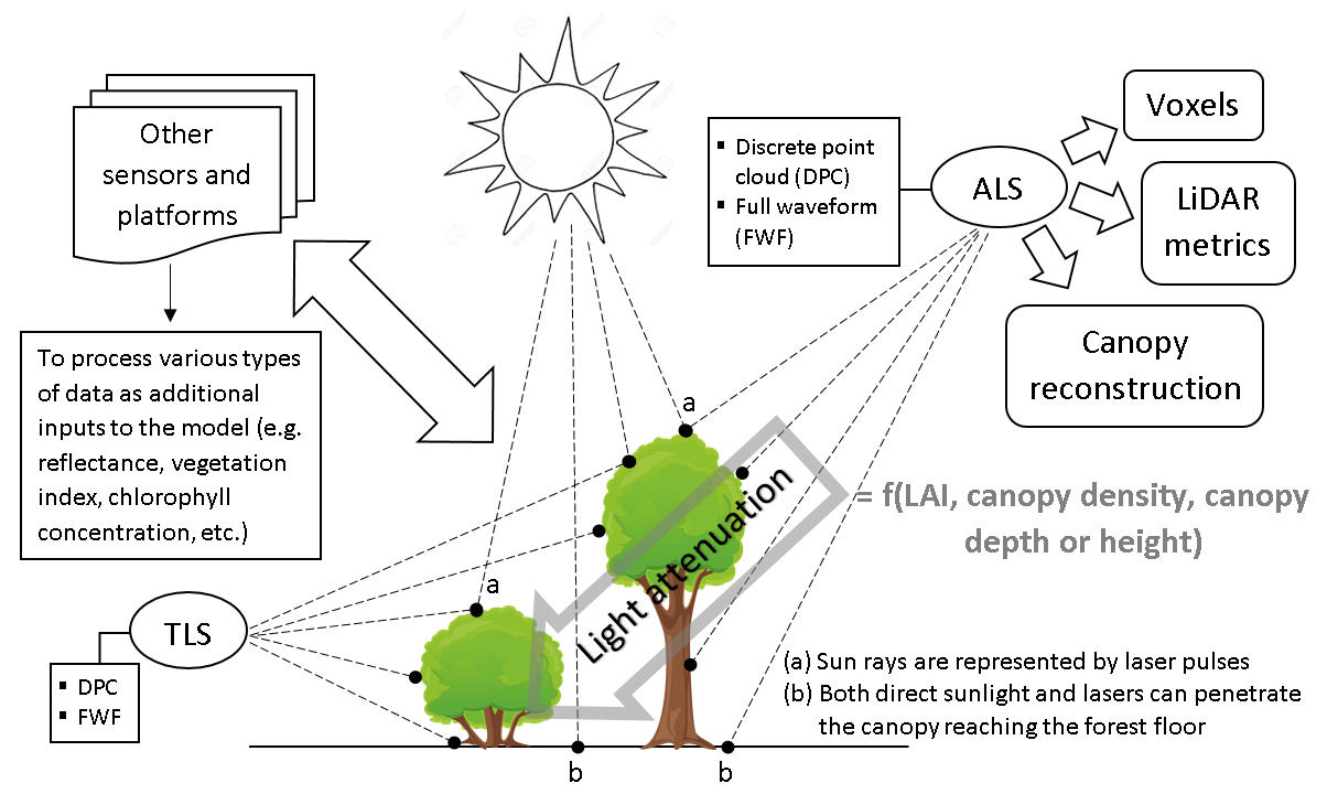
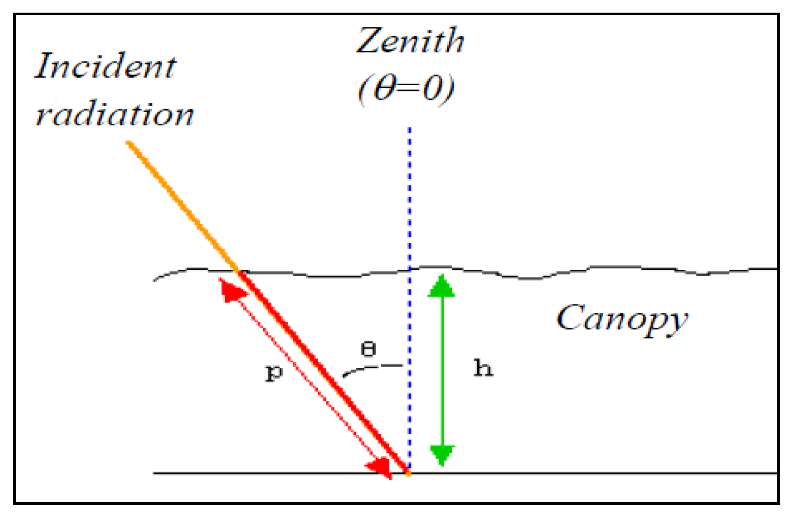
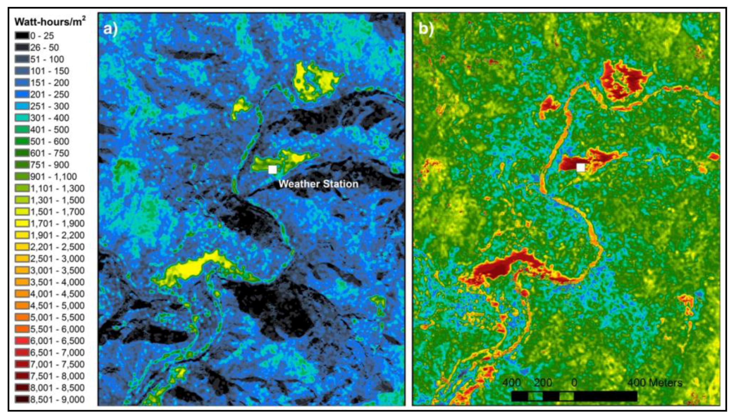
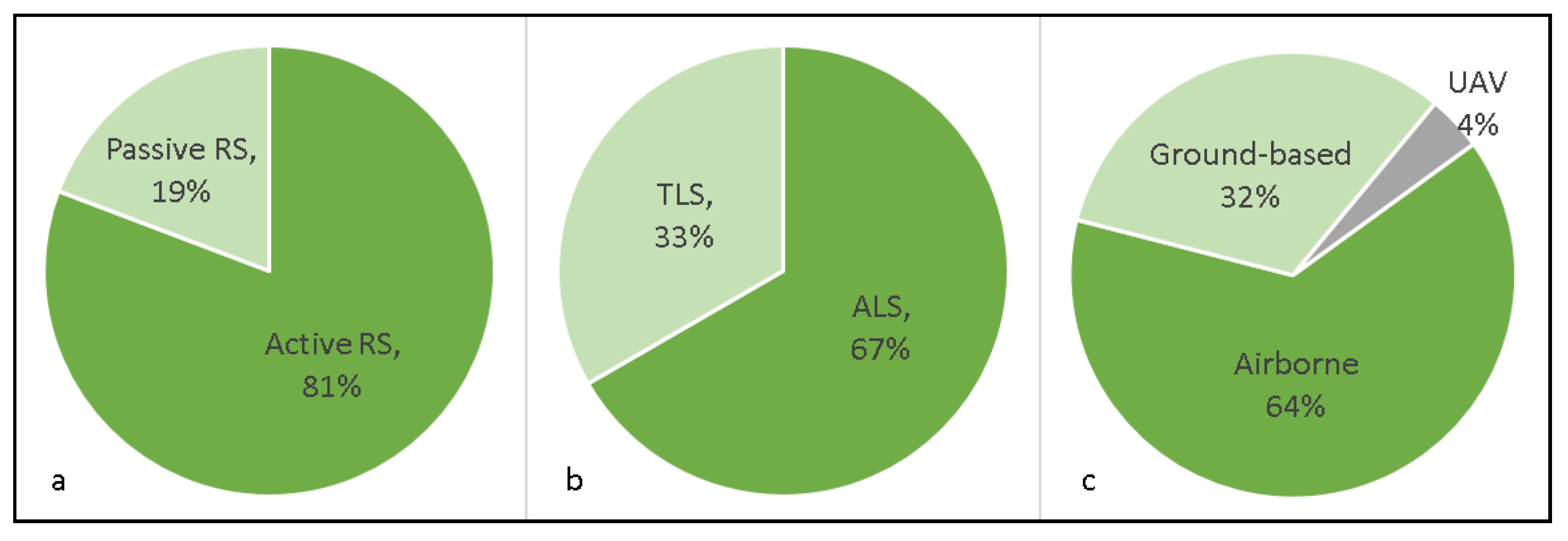
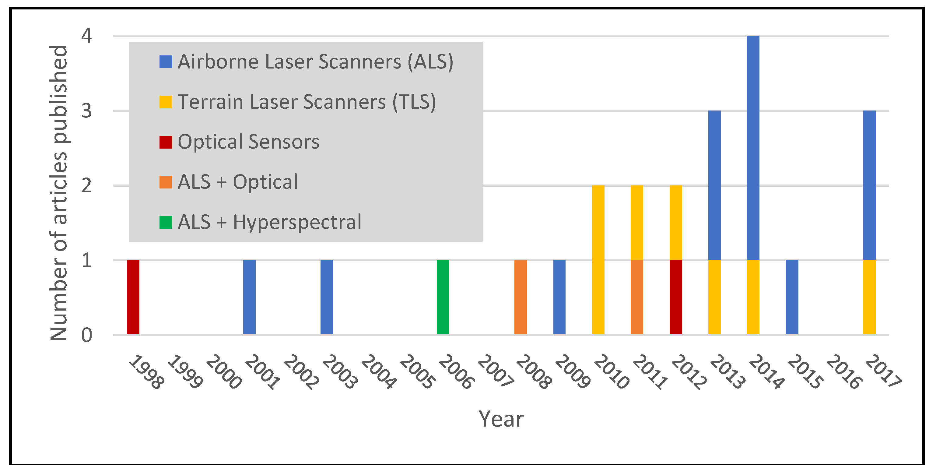
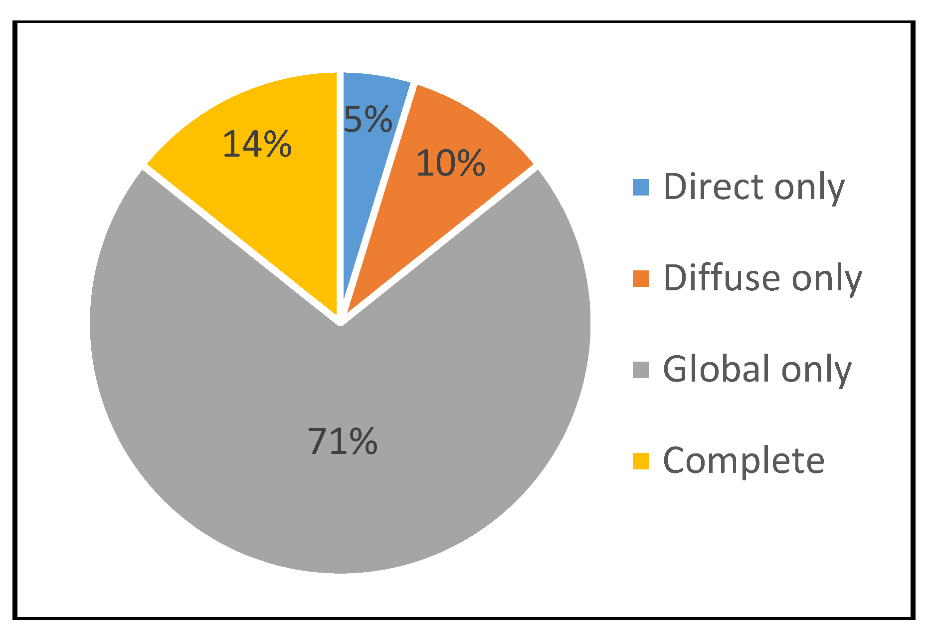
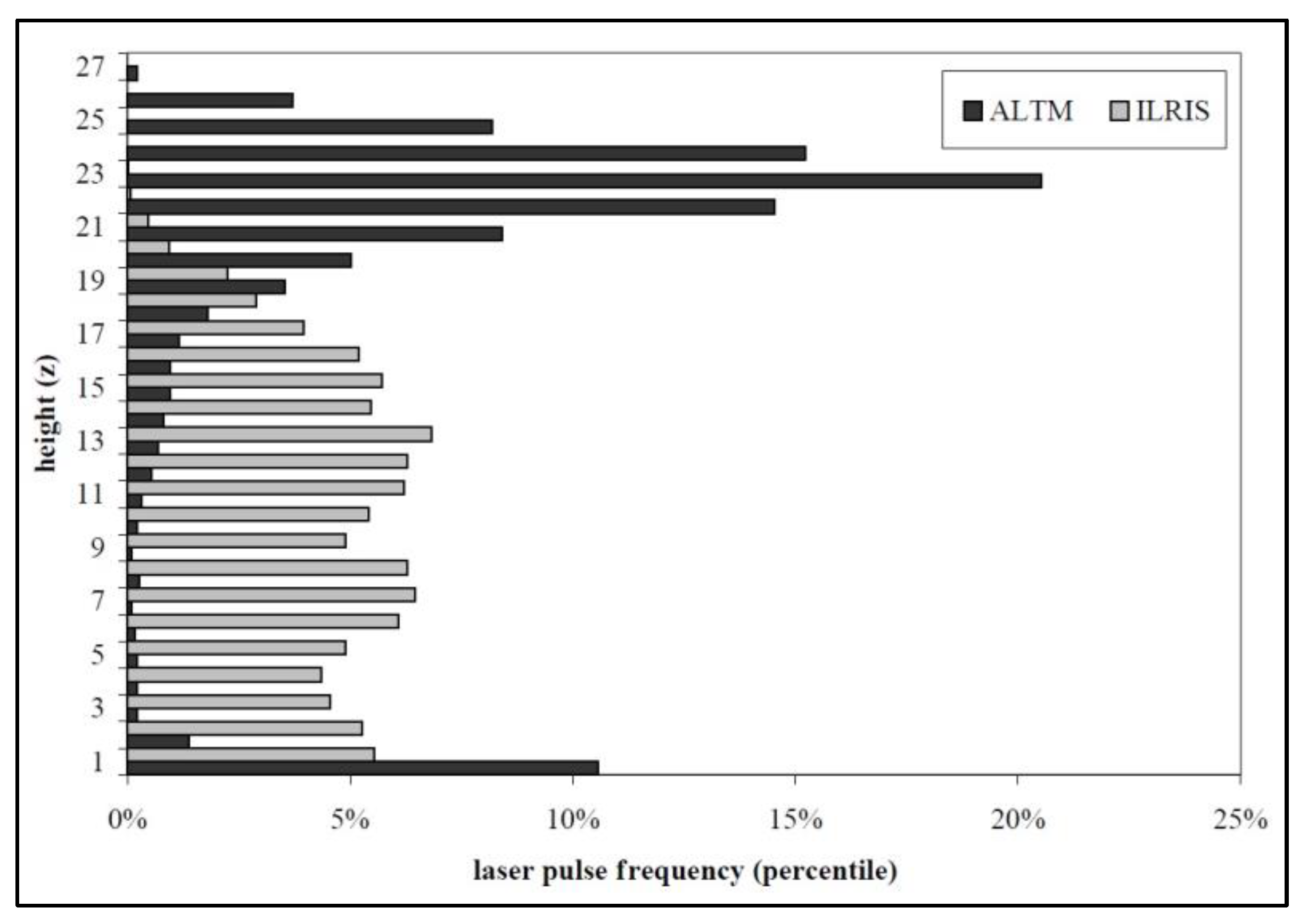
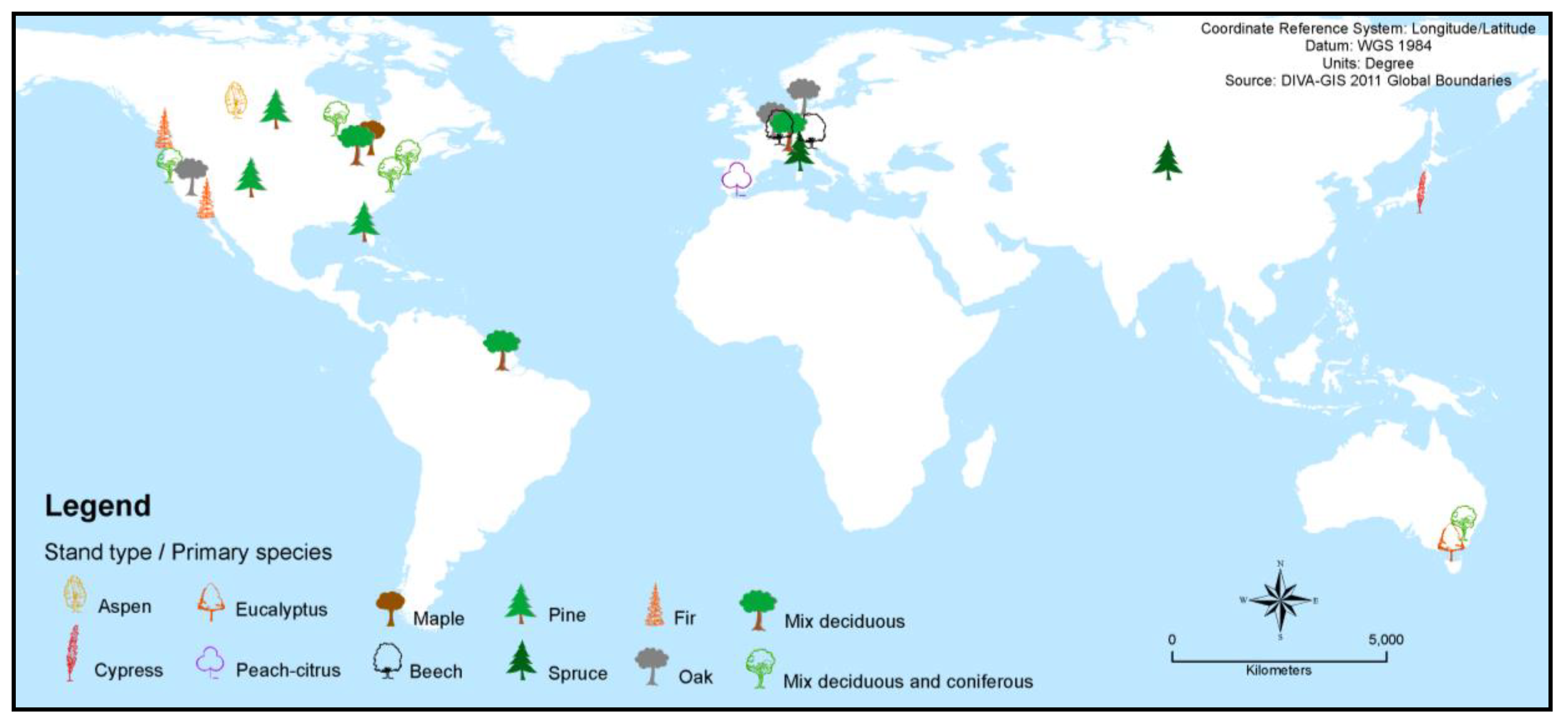
Table 1.
Studies on solar radiation below canopy utilizing remote sensing or allied sciences.
| References | Salient Methodology Features |
|---|---|
| Nyman et al., 2017 [55] | ▪ Compared various transmission models including a light penetration index (LPI) with a weighing factor to account for the path length |
| Tymen et al., 2017 [95] | ▪ Developed light transmission model using voxels generated from point clouds ▪ Used LPI |
| Cifuentes et al., 2017 [99] | ▪ Voxel-based canopy modeling generated from terrestrial laser system (TLS) ▪ Classified point clouds into leaves and non-leaves, then assigned properties before conducting light simulation |
| Yamamoto et al., 2015 [84] | ▪ Utilized owned version of LPI then correlated with relative illuminance |
| Bode et al., 2014 [22] | ▪ Used LPI and solar radiation module of GRASS software (r.sun) |
| Peng et al., 2014 [6] | ▪ Generated 3D canopy structure from point clouds ▪ Implemented Beer’s Law through voxel models with ray trace method |
| Moeser et al., 2014 [29] | ▪ Improvised synthetic hemispherical photos generated from point clouds |
| Widlowski et al., 2014 [25] | ▪ Voxel-based canopy reconstruction from TLS ▪ Bidirectonal reflectance factor (BRF) simulation in virtual environment |
| van Leeuwen et al., 2013 [34] | ▪ Used ground-based laser scanner Echidna Validation Instrument (EVI) to ▪ reconstruct geometric explicit models of canopy ▪ characterize radiation transmission properties from LiDAR full waveform |
| Musellman et al., 2013 [16] | ▪ Used Beer’s-type transmittance model based on LiDAR-derived LAI ▪ Developed solar raytrace model applied to 3D canopy derived from multiple LiDAR flights |
| Alexander et al., 2013 [21] | ▪ Estimated canopy cover by producing Thiessen polygons from point clouds ▪ Calculated canopy closure by transforming point clouds from Cartesian to spherical coordinates |
| Bittner et al., 2012 [67] | ▪ 3D voxel representation of the canopy architecture derived from TLS ▪ Different attributes of light assigned to voxels of stem, leaf or air |
| Guillen-Climent et al., 2012 [100] | ▪ Used a 3D radiative transfer model called forest light interaction model (FLIGHT) ▪ Mapped with high-resolution imagery from unmanned aerial vehicle (UAV) with multispectral camera |
| Kobayashi et al., 2011 [101] | ▪ Generated canopy height model, tree and crown segmentation from point clouds as inputs to CANOAK-FLiES (forest light environmental simulator) ▪ Derived canopy reflectance from airborne airborne visible/infrared imaging spectroradiometer (AVIRIS) |
| Van der Zande et al., 2011 [3] | ▪ Voxel-based representation of trees derived from TLS ▪ Light simulation using voxel-based light interception model (VLIM) |
| Van der Zande et al., 2010 [12] | ▪ Generate 3D representations of the forest stands, enabling structure feature extraction and light interception modeling, using the voxel-based light interception model (VLIM) |
| Yang et al., 2010 [75] | ▪ Estimated canopy gap probability from ground-based LiDAR (EVI) |
| Lee et al., 2009 [102] | ▪ Defined a conical field-of-view (scope) function between observer points just above the forest floor and the sun, which relates PAR to the LiDAR data |
| Essery et al., 2008 [85] | ▪ Colored orthophotograph and laser scanning were used to map out tree locations, heights, and crown diameter as inputs to mathematical radiation modeling and simulation |
| Thomas et al., 2006 [86] | ▪ LiDAR metrics generated from airborne laser system (ALS) to determine spatial variability of canopy structure ▪ Canopy chlorophyll concentration was derived from airborne hyperspectral imagery |
| Todd et al., 2003 [103] | ▪ Analyzed foliage distribution from LiDAR observation |
| Parker et al., 2001 [32] | ▪ Estimated canopy transmittance using the scanning LiDAR imager of canopies by echo recovery (SLICER), a waveform-sampling laser altimeter |
| Kucharik et al., 1998 [104] | ▪ Captured visible and NIR images of canopies from 16-bit charge-coupled device (CCD) multiband camera from the ground looking vertically upward to estimate sunlit and shaded foliage |
Table 2.
Selected countries with airborne LiDAR dataset available for public use.
© 2018 by the authors. Licensee MDPI, Basel, Switzerland. This article is an open access article distributed under the terms and conditions of the Creative Commons Attribution (CC BY) license (http://creativecommons.org/licenses/by/4.0/).
Share and Cite
MDPI and ACS Style
Olpenda, A.S.; Stereńczak, K.; Będkowski, K. Modeling Solar Radiation in the Forest Using Remote Sensing Data: A Review of Approaches and Opportunities. Remote Sens. 2018, 10, 694. https://0-doi-org.brum.beds.ac.uk/10.3390/rs10050694
AMA Style
Olpenda AS, Stereńczak K, Będkowski K. Modeling Solar Radiation in the Forest Using Remote Sensing Data: A Review of Approaches and Opportunities. Remote Sensing. 2018; 10(5):694. https://0-doi-org.brum.beds.ac.uk/10.3390/rs10050694
Chicago/Turabian StyleOlpenda, Alex S., Krzysztof Stereńczak, and Krzysztof Będkowski. 2018. "Modeling Solar Radiation in the Forest Using Remote Sensing Data: A Review of Approaches and Opportunities" Remote Sensing 10, no. 5: 694. https://0-doi-org.brum.beds.ac.uk/10.3390/rs10050694
Note that from the first issue of 2016, this journal uses article numbers instead of page numbers. See further details here.