Nowcasting Surface Solar Irradiance with AMESIS via Motion Vector Fields of MSG-SEVIRI Data

Abstract

In this study, we compare different nowcasting techniques based upon the calculation of motion vector fields derived from spectral channels of Meteosat Second Generation—Spinning Enhanced Visible and InfraRed Imager (MSG-SEVIRI). The outputs of the nowcasting techniques are used as inputs to the Advanced Model for Estimation of Surface solar Irradiance from Satellite (AMESIS), for predicting surface solar irradiance up to 2 h in advance. In particular, the first part of the methodology consists in projecting the time evolution of each MSG-SEVIRI channel (for every pixel in the spatial domain) through extrapolation of a displacement vector field obtained by matching similar patterns within two successive MSG-SEVIRI data images. Different ways to implement the above method result in substantial differences in the predicted trajectory, leading to different performances depending on the time interval of interest. All the nowcasting techniques considered here systematically outperform the simple persistence method for all MSG-SEVIRI channels and for each case study used in this work; importantly, this occurs across the entire 2 h period of the forecast. In the second part of the algorithm, the predicted irradiance maps computed with AMESIS from the forecasted radiances, are shown to be in good agreement with irradiances derived from MSG measured radiances and improve on numerical weather model predictions, thus providing a feasible alternative for nowcasting surface solar radiation. The results show that the mean values for correlation, bias, and root mean square error vary across the time interval, ranging between 0.94, −1 W/m${}^2$, 61 W/m${}^2$ after 15 min, and 0.73, −18 W/m${}^2$, 147 W/m${}^2$ after 2 h, respectively.

1. Introduction

Short-term forecast of cloud cover still poses a challenge to the scientific community, due to the inherent complexity and non-linearity of cloud motion in atmosphere [1,2,3,4,5,6,7]. This topic is of relevance to many fields, including solar energy production [4,8,9,10,11,12], since the presence of clouds has a significant impact on the stability and energy production of solar plants, causing dangerous fluctuations and great reduction to power supply [5]. Hence it is crucial to accurately monitor and forecast the position and trajectory of cloudy systems on very short-time scales. In the scientific literature this is referred to as nowcasting, i.e., short-term forecasting up to a few hours ahead (typically 0–2 h).

Many approaches for nowcasting have been proposed, which can be generally classified as statistical or physical/deterministic. Statistical techniques rely on a training process based on past datasets, and learn how to infer the evolution of weather parameters through identification of historical patterns. The simplest of these approaches is the persistence method, for which the current status is projected as is to the future; other statistical techniques include, but are not limited to, multivariate regression and neural network [13,14,15]. Among the physical approaches, cloud tracking techniques are applied by processing images from geostationary satellites [5,16,17,18], total sky imagery [19] or using other ground sensors [20]. In particular, satellite-based methods allow for global coverage, and high quality images are nearly continuously available. Satellite imagery is currently exploited to derive Atmospheric Motion Vectors [21] (AMVs, i.e., wind vector) as well as Cloud Motion Vectors (CMVs) [22,23,24]; these are obtained by analysing successive satellite images searching for the same features and to extrapolate the future trajectory on the basis of the recent past motion. The feature matching among subsequent images is performed by maximizing a pre-determined measure of similarity, which is typically either a correlation coefficient or the inverse of a mean square error. This technique was first implemented in [5] using a cross-correlation coefficient, similarly to [16], showing an improvement over the simple persistence method. In [17] a cloud-tracking technique is applied to Meteosat images using a probabilistic prediction for the cloud cover; many improvements have been proposed since then [18,25,26,27]. In [28,29] a variational method is used to minimise an energy like objective function incorporating the relevant features of the images analysed, while in [30] a disparity vector field for each pixel is used to perform the forecast. A huge body of literature can also be found on similar approaches, referred to as optical flow methods (see pioneer works [31,32]), which are typically applied in computer vision techniques; in practice these methods consist in the estimation of the distribution of brightness patterns of an image. A comprehensive description and analysis of these methods can be found in [4], in which an hybrid approach combining block-matching methods [16,33,34] and variational optical flow is implemented.

In this work, we exploit observations from Spinning Enhanced Visible and InfraRed Imager (SEVIRI) aboard the Meteosat Second Generation (MSG) geostationary satellite. We perform nowcasting of MSG-SEVIRI IR/VIS channels up to 2 h, by deriving motion vector fields in analogy to optical flow methods and cloud motion vector techniques. The forecasted radiances are then used as inputs to the Advanced Model for Estimation of Surface solar Irradiance from Satellite (AMESIS) [35] to predict surface solar irradiance maps. We extrapolate the motion with three different methods, compute the forecasted irradiance with AMESIS (using the forecasted radiances as input), and compare against the observed irradiance, derived with AMESIS from MSG measured radiances. To evaluate the degree of accuracy, we also include in the comparison the irradiance obtained with benchmarking methods such as simple persistence and the Weather Research and Forecasting (WRF) model [36] (see Appendix A for further details on the implementation of the model in this context). We emphasize that in this work we directly forecast MSG-SEVIRI IR/VIS radiances, while previous implemented satellite-based methods [37,38,39,40,41] generally pre-process the satellite images (e.g., to derive cloud index or cloud optical thickness maps), which then undergo an advection process to forecast the future position of cloud patterns. To summarise, the rationale for this work is twofold: i) to investigate and compare the performances of three variants of cloud motion technique, applied directly to the radiances measured by MSG-SEVIRI channels and ii) to define a self-consistent methodology providing nowcasting (up to 2 h) of surface solar irradiance maps, based on the integration of advection techniques and AMESIS.

The paper proceeds as follows: in Section 2 we present the methodology adopted in this work, by firstly (Section 2.1) analysing and comparing three variants of the cloud motion technique (used here to advect the radiance values of MSG-SEVIRI channels) and secondly (Section 2.2) by describing the AMESIS model used here to nowcast irradiance. In Section 3 we compare the statistical performances of each nowcasting variant previously discussed, and use the most accurate one for predicting solar irradiance maps with AMESIS; the results are then evaluated against the AMESIS-based MSG measurements and the WRF-based irradiance forecast. In Section 4 we finally draw our conclusions.

2. Materials and Methods

The method we use to forecast solar irradiance at the surface exploits the image data produced by the SEVIRI radiometer aboard the MSG geostationary satellite. MSG-SEVIRI scans the Earth’s full disk every 15 min, representing a valuable resource for cloud monitoring and tracking. SEVIRI is a multispectral imager, featuring twelve bands from the Visible (three channels) to the InfraRed (nine channels) regions of the electromagnetic spectrum. Here, we only consider the eleven channels with $3\mathrm{km}$ sub-point satellite resolution, thus neglecting the $1\mathrm{km}$ High Resolution Visible (HRV) channel. While the methodology could be easily extended to incorporate the HRV data, we decided not to for a fair comparison with the WRF model, that is run on a $3\mathrm{km}\times 3\mathrm{km}$ grid.

The variables adopted in this work to seed the nowcasting process are the radiance $L_{\mathrm{e}}$ from the first three (VIS/NIR) channels and the brightness temperature $T_{\mathrm{b}}$ from the eight (IR) channels; in this work we shall henceforth refer to both $L_{\mathrm{e}}$ and $T_{\mathrm{b}}$ as ‘radiances’, unless specified otherwise. Every pixel within the spatial domain under analysis is therefore associated with eleven values, corresponding to three $L_{\mathrm{e}}$ and eight $T_{\mathrm{b}}$. Based on these data at time $t_0$ and previous time $t_0-\Delta t$ (with time interval $\Delta t=15\min$), the aim is to perform a forecast of $L_e$ and $T_b$ for each pixel, at subsequent times $t_0+n\Delta t$ (with integer values $1\le n\le 8$), i.e., up to 2 h ahead. The predicted values for $L_e$ and $T_b$ are then used as inputs into AMESIS, to produce surface solar irradiance forecast every 15 min, with 2 h time horizon. We analysed day-time scenarios, selecting the following 24 days in 2017: 01-02-03-11-14-15-24-25-26-27-28 April; 01-03-10-11-12-22-31; June 04-10-25-27-28-30 May. For each of these days we provide nowcasting in two temporal intervals, i.e., during the morning (between 08:15 and 10:00 UTC) and in the afternoon (between 13:15 and 15:00 UTC), using SEVIRI data at 07:45 (This time corresponds to $t_0-\Delta t$ in the nowcasting scheme described in Section 2.1) and 08:00 (This time corresponds to $t_0$ in the nowcasting scheme described in Section 2.1) UTC for the morning, and 12:45 (This time corresponds to $t_0-\Delta t$ in the nowcasting scheme described in Section 2.1.) and 13:00 (This time corresponds to $t_0$ in the nowcasting scheme described in Section 2.1) UTC for the afternoon. The nowcasting of solar irradiance is therefore provided every 15 min and up to 2 hour time horizon, for the whole set of 48 case studies. We tested our methodology on a geographic area including most of the Italian peninsula, within the ranges of North latitude [${37.5}^{\circ }$, ${46.1}^{\circ }$], and East longitude [7.5${}^{\circ }$, 18.2${}^{\circ }$]. The method is applied on the entire domain consisting of 79616 pixel ($311\times 256$), with approximately $4\mathrm{km}\times 5\mathrm{km}$ typical resolution in the considered latitude range. The statistical analysis however focusses on a central inner grid ($257\times 202$ pixel) for reasons due to boundary conditions, as explained in Section 2.1.

In this section, we describe the algorithm used throughout this work, which essentially rests upon (i) a nowcasting scheme to predict the radiances on each channel and for every pixel of the spatial domain of interest, and (ii) the AMESIS product to calculate the solar irradiance for the corresponding pixels, based on the input forecasted values of $L_{\mathrm{e}}$ and $T_{\mathrm{b}}$. It is worth mentioning that the two parts are self-consistent: the first one (the nowcasting scheme, discussed in Section 2.1) yields forecasted values of $L_{\mathrm{e}}$ and $T_{\mathrm{b}}$, by means of advection techniques applied to the MSG-SEVIRI channels, while the second one (the AMESIS package described in Section 2.2) is a stand-alone model designed to monitor and calculate solar irradiance maps at the surface. We emphasize that the novelty feature in this work is twofold. On one hand we describe and compare different nowcasting techniques to directly advect $L_{\mathrm{e}}$ and $T_{\mathrm{b}}$ for every MSG-SEVIRI channel, whereas previous works focus on the advection of a posteriori derived features, such as the cloud index. On the other hand, the AMESIS software is proved to work in nowcasting mode, rather than real-time monitoring (as already demonstrated in [35]). We should further stress that while nowcasting of irradiance is usually performed by projecting the irradiance maps forward in time, in this work the irradiance forecast is calculated on the basis of the predicted values of $L_{\mathrm{e}}$ and $T_{\mathrm{b}}$.

2.1. Part I: The Nowcasting Process

The general approach to extrapolate the future motion of clouds, based upon matching the same feature between two (or more) consecutive data images, can be implemented in several ways, depending upon the required level of optimisation and the selected correlation criterion among the features. To derive displacement vectors to forward the trajectory of clouds in time and space, we adopt a technique that is similar in spirit to an optical flow method, however implementing a few refinements, which are discussed below. The core of the proposed nowcasting technique consists in extrapolating the time and spatial evolution of radiance maps (for each of the eleven channels taken into account) by projecting the motion observed between the actual time ($t_0$) and the previous time step ($t_0-\Delta t$).

Let us first describe the method to find the displacement between times $t_0-\Delta t$ and $t_0$. For each channel we initially select a squared ‘target’ area in the data image at time $t_0-\Delta t$, and a wider squared ‘search’ area (surrounding symmetrically the target area region) in the image at time $t_0$; the sizes of target and search areas are defined from the outset. To find the displacement of the pixel centered within the target area, between times $t_0-\Delta t$ and $t_0$, we follow a variational procedure. This consists in finding—inside the search area at time $t_0$—the target area that minimises the Mean Square Error (MSE) against the target area at time $t_0-\Delta t$. This process then yields the displacement vector from the pixel located in the center of the target area at time $t_0-\Delta t$, to the central pixel of the matching target area at time $t_0$ (see Figure 1). Finally, by scanning over the whole spatial domain, and iterating this process, we derive a displacement field for all pixels. Importantly, the size of the target and search areas are dependent upon each other; we found the optimum values to be 5 and 19 pixels for each side of the square-shaped target and search areas, respectively. The chosen target size is a good compromise for capturing large structures motion as well as small details dynamics; besides, the search area size allows for those features to travel at a reasonable maximum speed [42]. Please note that in our approach there is no distinction between clear and cloudy pixels (i.e., no cloud mask is used in the process); the algorithm relies solely on the radiance maps measured by SEVIRI, unlike previous works that deal with specific a posteriori derived parameters (e.g., cloud optical thickness or cloud index).

A few technical issues may arise when applying the technique as above. Firstly, it is unlikely that the variational procedure will yield a one-to-one correspondence, as it may occur that the same target area at time $t_0$ matches several target areas at time $t_0-\Delta t$. As a consequence, some pixels may be allocated with several radiance values whereas others remain ‘empty’; this non-injectivity issue is circumvented by using the mean of the several allocated radiance values in the first case, while reassigning the corresponding value from the previous time step and averaging over the neighbour pixels in the second case, respectively. While this may result in a somewhat crude approximation, we typically find that only a low percentage (less than $5\%$) of the pixels are affected by the above degeneracy. Secondly, cloudy systems may enter the considered spatial domain from outside the grid borders; to overcome this issue we define and focus on a smaller inner grid (which is the area of interest) within the analysed spatial domain, so that cloudy systems along the outer edges are usually buffered by the borders surrounding the inner area of interest.

The first step described so far strongly depends on the choice of the size of target and research areas, as well as the type of similarity measurement criterion for computing the correlation (here defined as the MSE). The second step features different ways to extrapolate the subsequent motion for every pixel, each of these leading to a different outcome. We now describe how these differences arise. At the end of the variational process discussed above, each pixel may be actually associated with a in and a out displacement vector, referring to the incoming direction of the radiance value entering the pixel and the outgoing direction of the radiance value leaving the pixel, respectively (Figure 2a). In case these two displacements differ (as in the example shown in Figure 2a), the forwarded trajectory becomes dependent on the type of displacement one decides to carry on in order to extrapolate the future motion. To take this subtlety into account, we have investigated and compared three types of forecast, here referred to as out, in and hybrid (Figure 2b).

In the out type, we can think of the grid as a fixed frame of reference and for each pixel consider only the outgoing (out) displacement. In this framework, which is closely related to the Atmospheric Motion Vector approach, each location can be thought as associated with a definite intensity and direction of a local wind, and consequently each radiance value is displaced accordingly. This approach is implemented by iterating the following equation, where $\Delta y_{(\mathrm{i},\mathrm{j})}^{{}^{\left(\mathrm{out}\right)}}$ and $\Delta x_{(\mathrm{i},\mathrm{j})}^{{}^{\left(\mathrm{out}\right)}}$ are the components (over the latitude and longitude directions, respectively) of the outgoing (out) displacements of the radiance from the pixel location $(i,j)$:

$$T_{\mathrm{b}}(i+\Delta y_{(\mathrm{i},\mathrm{j})}^{{}^{\left(\mathrm{out}\right)}},j+\Delta x_{(\mathrm{i},\mathrm{j})}^{{}^{\left(\mathrm{out}\right)}},t_0+n\Delta t)=T_{\mathrm{b}}(i,j,t_0+(n-1)\Delta t)$$

(1)

Please note that the indices span the ranges $1\le i\le 256$ and $1\le j\le 311$ within the spatial domain of interest. In the in type, we deal with a moving frame of reference, as we closely follow the path of each radiance value starting from the initial incoming (in) displacement. In this framework, each radiance value can be thought of as a particle featuring its own motion, and the iteration describing its evolution is as follows (where $\Delta y_{(\mathrm{i},\mathrm{j})}^{{}^{\left(\mathrm{in}\right)}}$ and $\Delta x_{(\mathrm{i},\mathrm{j})}^{{}^{\left(\mathrm{in}\right)}}$ are obtained by averaging over the several in displacements found in the variational procedure, and refer to the incoming (in) displacements):

$$T_{\mathrm{b}}(i+n\Delta y_{(\mathrm{i},\mathrm{j})}^{{}^{\left(\mathrm{in}\right)}},j+n\Delta x_{(\mathrm{i},\mathrm{j})}^{{}^{\left(\mathrm{in}\right)}},t_0+n\Delta t)=T_{\mathrm{b}}(i+(n-1)\Delta y_{(\mathrm{i},\mathrm{j})}^{{}^{\left(\mathrm{in}\right)}},j+(n-1)\Delta x_{(\mathrm{i},\mathrm{j})}^{{}^{\left(\mathrm{in}\right)}},t_0+(n-1)\Delta t)$$

(2)

The third type, hybrid, is a linear combination of the out and in ones, based on a displacement for each pixel obtained as the mean of the incoming and outgoing displacements (i.e., $\Delta y_{(\mathrm{i},\mathrm{j})}^{\mathrm{hybr}}=[\Delta y_{(\mathrm{i},\mathrm{j})}^{{}^{\left(\mathrm{in}\right)}}+\Delta y_{(\mathrm{i},\mathrm{j})}^{{}^{\left(\mathrm{out}\right)}}]/2$ and $\Delta x_{(\mathrm{i},\mathrm{j})}^{\mathrm{hybr}}=[\Delta x_{(\mathrm{i},\mathrm{j})}^{{}^{\left(\mathrm{in}\right)}}+\Delta x_{(\mathrm{i},\mathrm{j})}^{{}^{\left(\mathrm{out}\right)}}]/2$ ), yielding the following equation:

$$T_{\mathrm{b}}(i+\Delta y_{(\mathrm{i},\mathrm{j})}^{{}^{\left(\mathrm{hybr}\right)}},j+\Delta x_{(\mathrm{i},\mathrm{j})}^{{}^{\left(\mathrm{hybr}\right)}},t_0+n\Delta t)=T_{\mathrm{b}}(i,j,t_0+(n-1)\Delta t)$$

(3)

It should be noticed that in all former equations the brightness temperature $T_{\mathrm{b}}$ is to be replaced by the radiance $L_{\mathrm{e}}$ when considering the VIS/NIR bands. For each variant presented above, we also consider its smoothed counterpart: this is derived by averaging (every time step) the radiance value in each pixel with its surrounding eight neighbours. In Section 3 we demonstrate that the above three variants (together with their smoothed counterparts) lead to an overall good agreement with SEVIRI measurements, within the first two hours of forecast horizon.

2.2. Part II: AMESIS

The second part of the algorithm discussed in this work is based on AMESIS; in this section we therefore provide a brief overview of this model (for further details see [35]). As discussed in Section 2.1, the first part of the solar irradiance nowcasting algorithm yields the predicted values for radiance on each of the eleven SEVIRI spectral channels and for every pixel within the spatial domain under analysis; the second part, entirely based on AMESIS, takes as inputs the predicted $L_{\mathrm{e}}$ and $T_{\mathrm{b}}$, and computes estimates for surface solar irradiance values at each pixel location. AMESIS was proved to work for surface solar irradiance monitoring purposes in the region 33–60 degrees North and 11–30 degrees East, for every season, different sun zenith angles, radiance ranges and albedo. AMESIS exploits MSG-SEVIRI data, ingesting near-real-time 15 min resolution SEVIRI spectral images. In this work, the use of AMESIS has been extended to nowcasting, i.e., by ingesting predicted values of SEVIRI radiance to provide surface solar irradiance forecast within 2 h time horizon. AMESIS starts with the pixel classification as clear, cloudy, partially cloudy, or affected by aerosol presence, exploiting Cloud Mask Coupling of Statistical and Physical methods (C-MACSP) algorithm [43]. Except for pixels detected as clear, the model retrieves the microphysical optical parameters for clouds or aerosol. Subsequently the model retrieves the surface solar irradiance on the basis of look-up tables that are periodically updated. Therefore AMESIS incorporates the effects due to aerosol, overcast and partially cloudy coverage; the retrieval of surface temperature, total integrated water vapour, cloud and aerosol microphysical parameters is fulfilled by using VIS and IR SEVIRI channels, whereas surface solar irradiance can be retrieved either with the low-resolution VIS channels or through the HRV, depending on the desired resolution. As anticipated earlier, the SEVIRI-HRV channel is not used here, and thus AMESIS is run in low-resolution mode, allowing direct comparison with the WRF model output, also implemented on a $3\mathrm{km}\times 3\mathrm{km}$ grid.

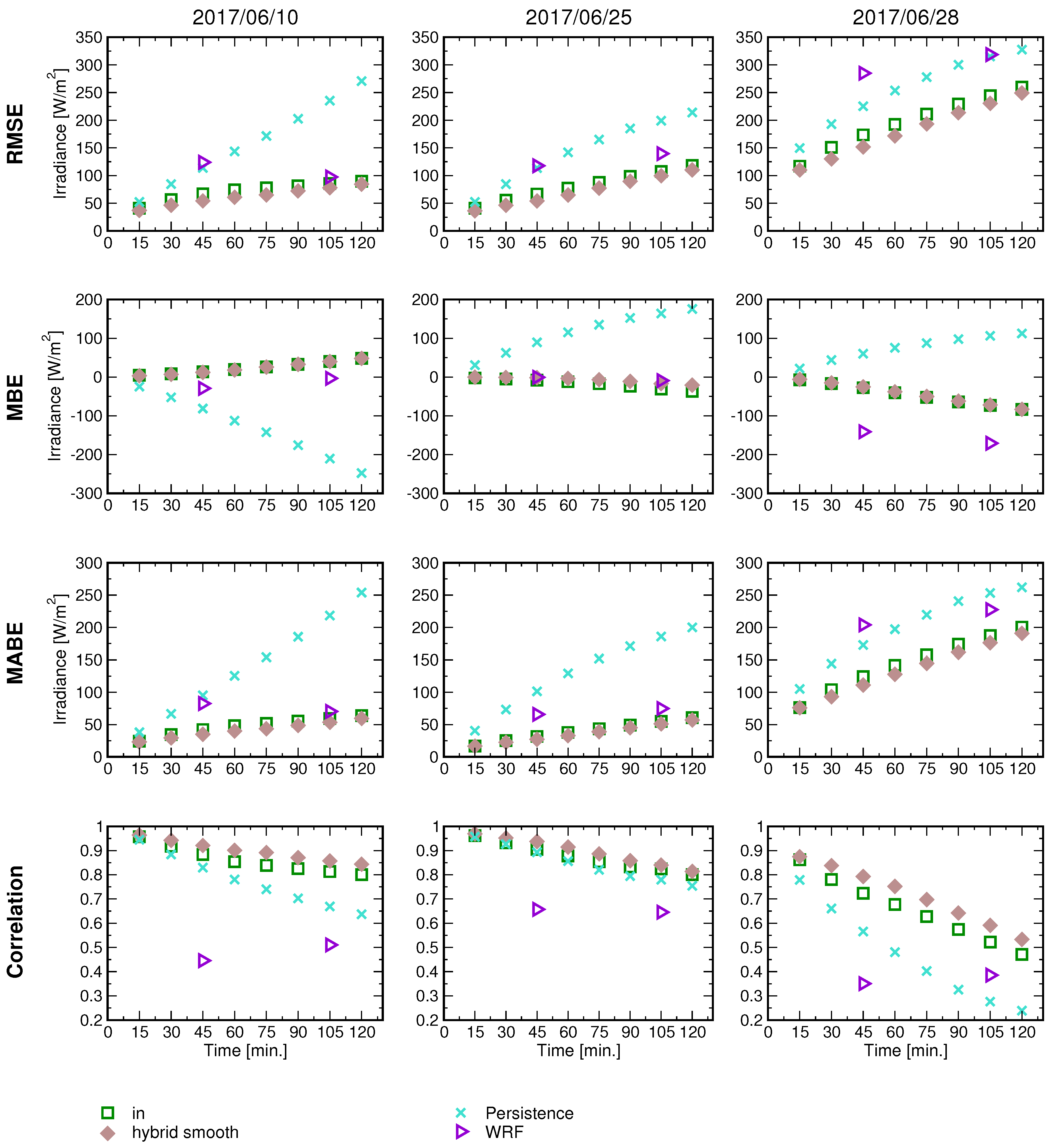
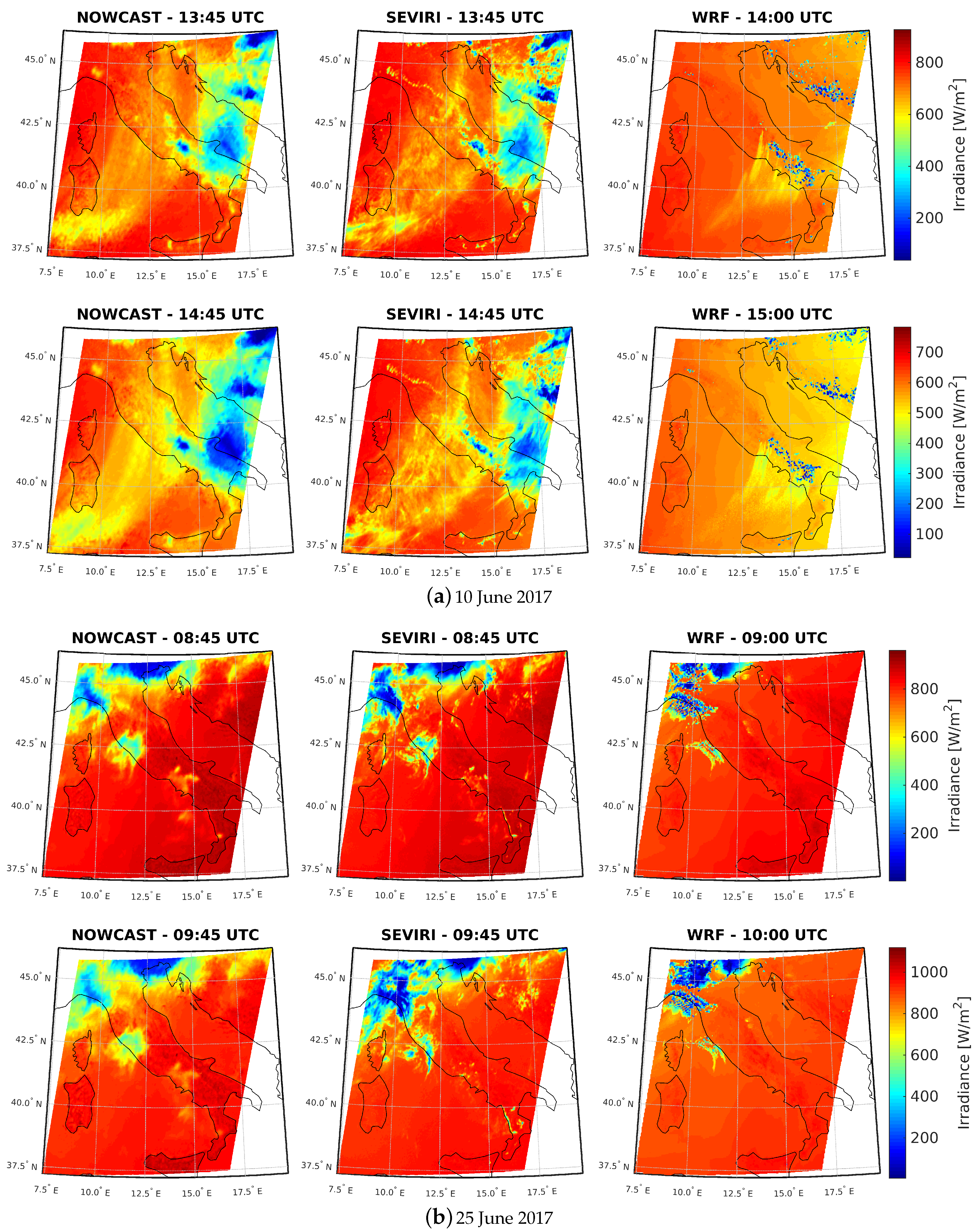
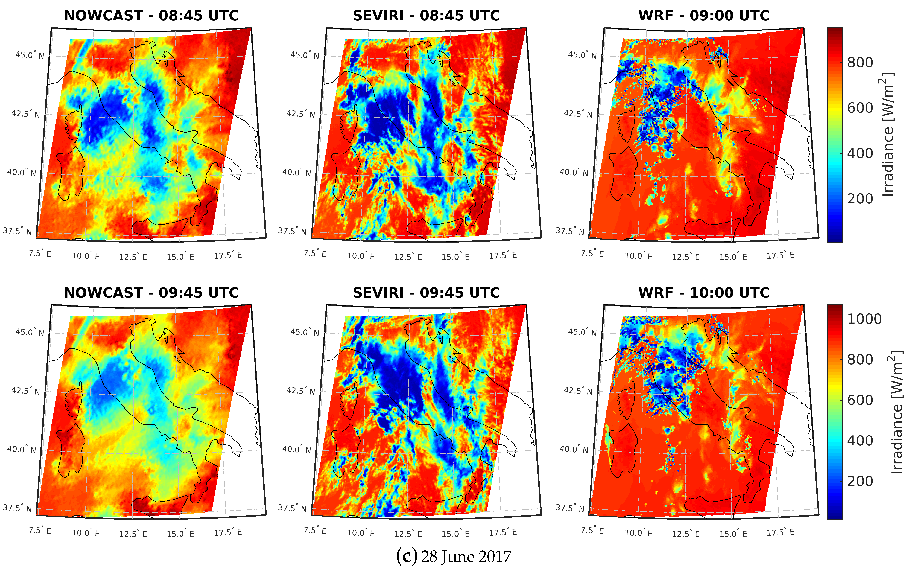
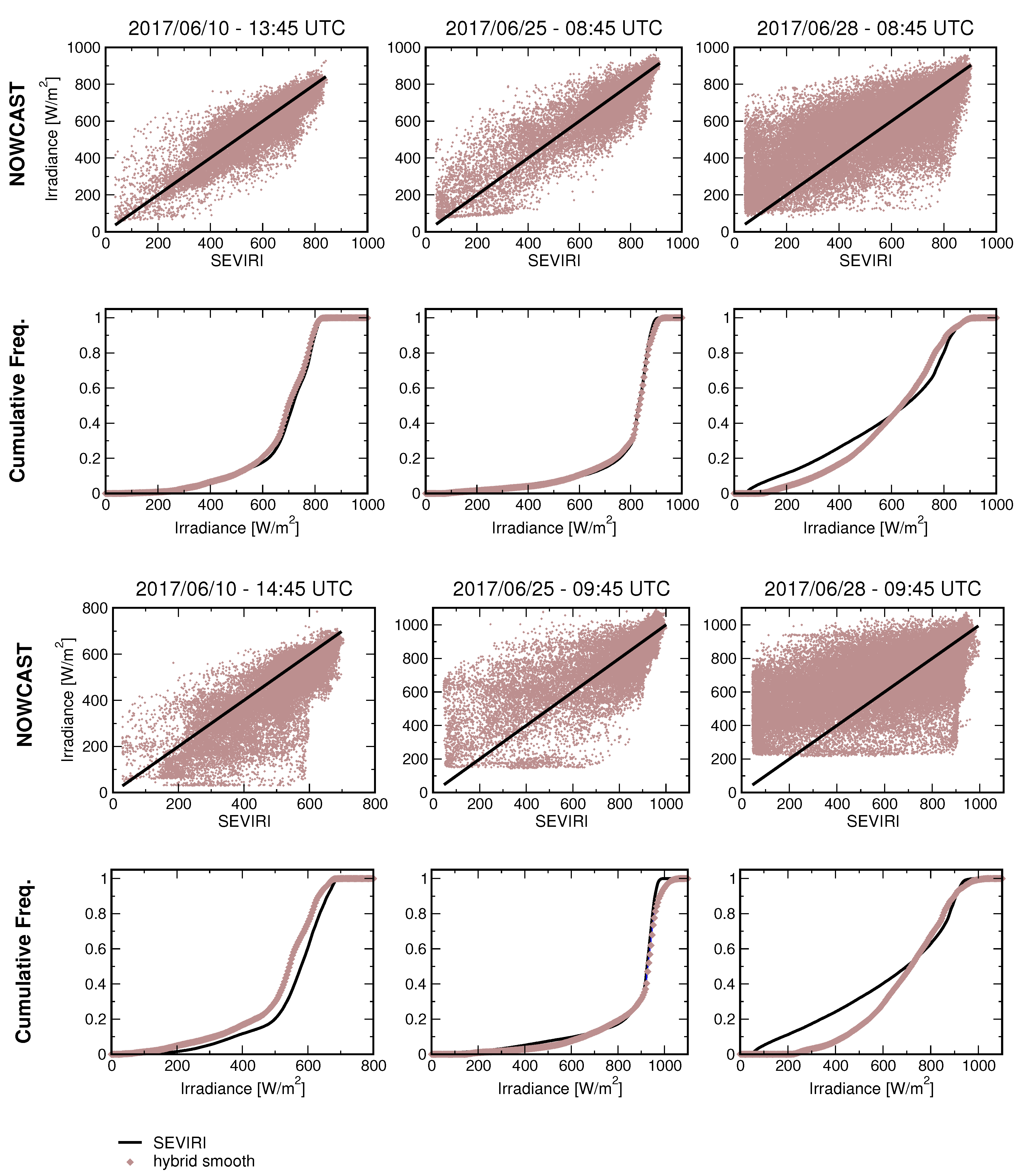
3. Results and Discussion

The treatment discussed in Section 2.1 is based solely on simple advection of the MSG-SEVIRI channels, thus neglecting convective processes as well as dissipative mechanisms. For this reason the quality of the algorithm has been evaluated by selecting a dataset mainly featuring broken clouds, avoiding unstable atmospheric conditions possibly causing convective initiation. We emphasize that the selected conditions (partially cloudy) heavily affect the stability of photovoltaic systems, due to rapid changes in the solar irradiance intensity.

The output of the first part of the algorithm is analysed by comparing the six variants discussed in Section 2.1, against the MSG-SEVIRI measured values; we also include in the comparison the simple persistence model (here implemented by keeping the $t_0$ MSG-SEVIRI channels radiance values across the entire time interval). Figure 3 shows the statistical analysis by means of the Root Mean Square Error (RMSE), Mean Bias Error (MBE) and Correlation for the two visible channels (Ch. 1, 2), the near-infrared (Ch. 4) and two infrared channels (Ch. 6, 10). In this work the BIAS is computed as the mean of the differences between the forecast and MSG measured radiances for every pixel; the MBE is obtained as the average of the BIAS over the whole sample of 48 case studies. It is worth noticing that these channels are the most relevant ones for the calculation of the solar irradiance through AMESIS. The simple persistence model is outperformed (in terms of both RMSE and Correlation) by all the other methods, at all times within the forecast interval. The improvement relative to the persistence model is negligible at the first nowcasting time step (i.e., after 15 min) and increases with time. Figure 3 shows that the hybrid smooth is the most performing among the variants in terms of RMSE and Correlation; for all channels the correlation ranges between the maximum value of 0.97 and the minimum value of 0.7 within the 2 h of prediction. However the hybrid smooth reveals a relatively higher bias compared to the other variants, while the in variant minimises the BIAS for the visible bands (Ch. 1, 2). We point out that the analysis is based on the average over the whole dataset (48 case studies) considered in this work, and concerns the estimate of radiances in each pixel and for every SEVIRI channel. Finally, the first stage of the algorithm (i.e., the nowcasting process) revealed the following: (i) all of the variants used here show very good agreement with the MSG-SEVIRI measured values of radiances for each channel (e.g., correlation is greater than 0.7 even after 2 h of nowcasting); (ii) all the methods clearly show very similar trends, improving on the predictions provided by the simple persistence model; (iii) relative to the visible bands (Ch. 1–2) the hybrid smooth and the in approaches are the most performing variants in terms of RMSE/Correlation and Bias, respectively. For the reasons above, in the second part of the algorithm we use both in and hybrid smooth based outputs, as inputs in AMESIS for the estimation of surface solar irradiance.

To characterise the second part of the algorithm (described in Section 2.2) and evaluate its performance, we have selected three particular case studies: these feature the lowest (10 June 2017, afternoon), intermediate (25 June 2017, morning) and highest (28 June 2017, morning) RMSE value for the forecasted radiances of the SEVIRI visible channels, according to the hybrid smooth performance in the nowcasting scheme analysis. We therefore expect a direct relation with the AMESIS solar irradiance output, such that the aforementioned case studies will prove to be the best, intermediate, and worst irradiance forecast within the dataset, respectively. In Figure 4 we report the statistical analysis for the above case studies, comparing the irradiance predicted by means of the hybrid smooth and in nowcasting approaches against the benchmark models of simple persistence and WRF. The statistical measures are evaluated with respect to the irradiance calculated through AMESIS based on the MSG-SEVIRI measured radiances. We should also point out that solar irradiance predictions based on hybrid smooth, in and simple persistence approaches are obtained through AMESIS by using the corresponding forecasted radiances values as inputs, whereas the WRF solar irradiance is computed within the code using the model atmospheric variables to solve a parametrized radiative transfer (see Appendix A). We include the WRF prediction in the comparison analysis in order to quantify the potential improvement by using the nowcasting approach within the first two hours of forecast, instead of the WRF prediction. The WRF irradiance predictions are available on a hourly basis, at specific times, i.e., at 14:00 UTC and 15:00 UTC for the afternoon case on the 10 June 2017 and 09:00 UTC and 10:00 UTC for the morning cases on the 25 June 2017 and 28 June 2017. We compared the above against the time collocated nowcasting-based AMESIS predictions; the times selected for the comparison correspond to the 3rd (08:45 or 13:45 UTC) and 7th (09:45 or 14:45 UTC) temporal step of the hybrid smooth/in nowcasting process, i.e., after 45 and 105 min, respectively. The results shown in Figure 4 reveal the following: (i) the predictions based on the hybrid smooth method are more accurate then the predictions based on the in method; (ii) the irradiance forecasted with the benchmarks models feature a systematically higher RMSE and lower Correlation, at all times and in each case study; (iii) the correlation relative to the nowcasting methods proposed in this work is relatively stronger across the entire time interval; in the worst case scenario (28 June 2017) it reaches the lowest value of 0.52 only after two hours of forecast, whereas it ranges between 0.85–1 for the two other cases, hence demonstrating the robustness of the procedure. By combining the statistical scores of the hybrid smooth method, obtained for the three cases analysed in Figure 4, we find that the mean value ranges between 0.94 and 0.73 for correlation, between −1 W/m${}^2$ and −18 W/m${}^2$ for bias and between 61 W/m${}^2$ and 147 W/m${}^2$ for the rmse (values are calculated after 15 min and 2 h, respectively). In order to give a qualitative overview of the results, the corresponding irradiance maps are reported in Figure 5, where we compare the AMESIS-based hybrid smooth predictions (proved to be the best nowcasting method in this work) and the WRF calculated output, against the AMESIS-based SEVIRI measurements, for the three case studies analysed (10 June 2017; 25 June 2017; 28 June 2017). The results show that irradiance maps obtained through nowcasting (hybrid smooth) largely reproduce the SEVIRI observed results, however featuring smooth low-irradiance regions, as expected. The WRF results tend to underestimate the cloudy regions instead, and this occurs for all the case studies examined. We should further stress that the purpose of Figure 5 is only to provide a qualitative comparison of the irradiance maps obtained with nowcast, WRF and SEVIRI measurements, for the case studies analysed. One can clearly infer the distribution of cloudy systems (regions of relatively low irradiance) in the maps, and qualitatively evaluate whether the simulated patterns match the SEVIRI observations.

We now further investigate the statistics of the irradiance output derived with the most performing nowcasting method, namely the hybrid smooth; this is compared against the AMESIS-based irradiance derived with MSG-SEVIRI measured radiances, by evaluating scatter plots and cumulative frequency curves. In Figure 6 we show the scatter plots for the irradiances obtained with the nowcasting methodology, for the same case studies and times shown in Figure 5. We notice that nowcast predictions follow a regular distribution and feature a relatively low spread compared to the SEVIRI output, at the 3rd time step (i.e., after 45 min) of the nowcasting process. This is further supported by the cumulative frequency curves, also shown in Figure 6, which demonstrate a very good agreement between predictions and MSG measured values (except for the worst case scenario on 28 June 2017). As expected, the agreement and correlation between measured and simulated data tend to reduce after 105 min, at the 7th time step, as also shown in Figure 6. Based on the above outcome, the nowcasting approach described here may be used to complement the WRF solar irradiance prediction, especially within the first two hours forecast time. In such a way, a self-consistent approach providing an efficient monitoring, nowcasting up to 2 h and forecasting beyond 2 h of solar irradiance maps, is derived through the integration of AMESIS, cloud motion techniques, and WRF model.

4. Conclusions

In this work we present an algorithm for providing accurate short term forecast (0–2 h) of surface solar irradiance, based solely on the (i) advection of MSG-SEVIRI channels and (ii) Advanced Model for Estimation of Surface solar Irradiance from Satellite (AMESIS). The first part of the algorithm consists in an advecting technique (in analogy to optical flow methods) applied directly to the radiances and brightness temperatures of MSG-SEVIRI channels; we investigate different types of extrapolation (here referred to as out, in, hybrid), and select the best approach to feed AMESIS in the second part of the algorithm. For evaluation, we selected a set of 48 case studies, divided equally between day and afternoon, and featuring mainly broken clouds scenarios. The nowcasting of surface solar irradiance is provided every 15 min across the time intervals [08:15, 10:00] UTC for the morning cases and [13:15, 15:00] UTC for the afternoon ones.

The statistical analysis is based on the calculation of the RMSE, BIAS, MABE, Correlation, as well as scatter plots and cumulative frequency curves; each of these is evaluated with respect to MSG measured values and averaged over all samples. We find similar overall trend across the entire forecast time range for the nowcasting methods proposed here. However the hybrid smooth approach stands out for relatively higher (lower) values of Correlation (RMSE). Nonetheless all variants implemented show very good agreement with the outcome based on MSG-SEVIRI measurements, and improve on the results derived from benchmark models such as simple persistence and WRF models. This has been verified on the basis of the performance exhibited in the best (10 June 2017), intermediate (25 June 2017) and worst (28 June 2017) case scenarios relative to the RMSE. The correlation for the above cases varies on average between 0.94 after 15 min and 0.73 after 2 h, for the hybrid smooth nowcasting method. The corresponding range for the simple persistence method is [0.89, 0.54], while for the WRF model is on average 0.5 at all times examined.

The nowcasting approach described here is therefore proved to be a valid approach for short term (0–2 h) forecasting of solar irradiance. The treatment discussed however is based solely on advection and extrapolation of MSG-SEVIRI channels, thus neglecting convective processes and dissipative mechanisms. Further work foresees to incorporate the modeling of cloud growth and dissipation mechanisms, as well as of convection phenomena, useful for the forecasting of storm events.

References

1. Menzel, W.P. Cloud Tracking with Satellite Imagery: From the Pioneering Work of Ted Fujita to the Present. Bull. Am. Meteorol. Soc. 2001, 82, 33–47. [Google Scholar] [CrossRef]
2. Batlles, F.J.; Alonso, J.; López, G. Cloud Cover Forecasting from METEOSAT Data. Energy Procedia 2014, 57, 1317–1326. [Google Scholar] [CrossRef]
3. Arbizu-Barrena, C.; Ruiz-Arias, J.A.; Rodríguez-Benítez, F.J.; Pozo-Vázquez, D.; Tovar-Pescador, J. Short-term solar radiation forecasting by advecting and diffusing MSG cloud index. Sol. Energy 2017, 155, 1092–1103. [Google Scholar] [CrossRef]
4. Peng, Z.; Yu, D.; Huang, D.; Heiser, J.; Kalb, P. A hybrid approach to estimate the complex motions of clouds in sky images. Sol. Energy 2016, 138, 10–25. [Google Scholar] [CrossRef]
5. Leese, J.A.; Novak, C.S.; Clark, B.B. An Automated Technique for Obtaining Cloud Motion from Geosynchronous Satellite Data Using Cross Correlation. J. Appl. Meteorol. 1971, 10, 118–132. [Google Scholar] [CrossRef]
6. Bedka, K.M.; Velden, C.S.; Petersen, R.A.; Feltz, W.F.; Mecikalski, J.R. Comparisons of Satellite-Derived Atmospheric Motion Vectors, Rawinsondes, and NOAA Wind Profiler Observations. J. Appl. Meteorol. Climatol. 2009, 48, 1542–1561. [Google Scholar] [CrossRef]
7. Bedka, K.M.; Mecikalski, J.R. Application of Satellite-Derived Atmospheric Motion Vectors for Estimating Mesoscale Flows. J. Appl. Meteorol. 2005, 44, 1761–1772. [Google Scholar] [CrossRef]
8. Heinemann, D.; Lorenz, E.; Girodo, M. Forecasting of Solar Radiation. 2006. Available online: http://citeseerx.ist.psu.edu/viewdoc/download?doi=10.1.1.526.2530&rep=rep1&type=pdf (accessed on 25 May 2018).
9. Cebecauer, T.; Suri, M.; Perez, R. High Performance MSG Satellite Model for Operational Solar Energy Applications. ASES Ann. Conf. 2010. Available online: http://proceedings.ases.org/wp-content/uploads/2014/02/2010-086small.pdf (accessed on 25 May 2018).
10. Perez, R.; Kivalov, S.; Schlemmer, J.; Hemker, K.; Zelenka, A. Improving the Performance of Satellite-To-Irradiance Models Using the Satellite’s Infrared Sensors. In Proceedings of the 39th ASES National Solar Conference 2010, SOLAR 2010; Volume 1. Available online: http://proceedings.ases.org/wp-content/uploads/2014/02/2010-038small.pdf (accessed on 25 May 2018).
11. Perez, R.; Kankiewicz, A.; Schlemmer, J.; Hemker, K.; Kivalov, S. A New Operational Solar Resource Forecast Model Service for PV Fleet Simulation. 2014, pp. 0069–0074. Available online: http://www.asrc.albany.edu/people/faculty/perez/2014/fcst.pdf (accessed on 25 May 2018).
12. Pelland, S.; Remund, J.; Kleissl, J.; Oozeki, T.; De Brabandere, K. Photovoltaic and Solar Forecasting: State of the Art. 2013. Available online: https://www.nachhaltigwirtschaften.at/resources/iea_pdf/reports/iea_pvps_task14_report_2013_photovoltaic_and_solar_forecasting_state_of_the_art.pdf (accessed on 25 May 2018).
13. Mellit, A. Artificial Intelligence technique for modelling and forecasting of solar radiation data: A review. Int. J. Artif. Intell. Soft Comput. 2008, 1, 52–76. [Google Scholar] [CrossRef]
14. Pedro, H.T.; Coimbra, C.F. Assessment of forecasting techniques for solar power production with no exogenous inputs. Sol. Energy 2012, 86, 2017–2028. [Google Scholar] [CrossRef]
15. Marquez, R.; Gueorguiev, V.G.; Coimbra, C.F. Forecasting of Global Horizontal Irradiance Using Sky Cover Indices. ASME. J. Sol. Energy Eng. 2012, 135. Available online: https://pdfs.semanticscholar.org/12b0/b506a1b3d5eedcc9a749512b71026669ac29.pdf (accessed on 25 May 2018). [CrossRef]
16. Hamill, T.M.; Nehrkorn, T. A Short-Term Cloud Forecast Scheme Using Cross Correlations. Weather Forecast. 1993, 8, 401–411. Available online: https://www.esrl.noaa.gov/psd/people/tom.hamill/crosscorr_cloud.pdf (accessed on 25 May 2018). [CrossRef]
17. Hammer, A.; Heinemann, D.; Lorenz, E.; Lückehe, B. Short-term forecasting of solar radiation: A statistical approach using satellite data. Sol. Energy 1999, 67, 139–150. [Google Scholar] [CrossRef]
18. Lorenz, E.; Hammer, A.; Heinemann, D. Short term forecasting of solar radiation based on satellite data. In Proceedings of the EUROSUN2004 (ISES Europe Solar Congress), Freiburg, Germany, 20–23 June 2004. [Google Scholar]
19. Cheng, H.Y. Cloud tracking using clusters of feature points for accurate solar irradiance nowcasting. Renew. Energy 2017, 104, 281–289. [Google Scholar] [CrossRef]
20. Bosch, J.L.; Zheng, Y.; Kleissl, J. Deriving Cloud Velocity From an Array of Solar Radiation Measurements. Energy Sustain. 2012, 1059–1065. [Google Scholar] [CrossRef]
21. Velden, C.S.; Olander, T.L.; Wanzong, S. The Impact of Multispectral GOES-8 Wind Information on Atlantic Tropical Cyclone Track Forecasts in 1995. Part I: Dataset Methodology, Description, and Case Analysis. Mon. Weather Rev. 1998, 126, 1202–1218. [Google Scholar] [CrossRef]
22. Guillot, E.M.; Haar, T.H.V.; Forsythe, J.M.; Fletcher, S.J. Evaluating Satellite-Based Cloud Persistence and Displacement Nowcasting Techniques over Complex Terrain. Weather Forecast. 2012, 27, 502–514. [Google Scholar] [CrossRef]
23. Nonnenmacher, L.; Coimbra, C.F. Streamline-based method for intra-day solar forecasting through remote sensing. Sol. Energy 2014, 108, 447–459. [Google Scholar] [CrossRef]
24. Schroedter-Homscheidt, M.; Gesell, G. Verification of sectoral cloud motion based direct normal irradiance nowcasting from satellite imagery. AIP Conf. Proc. 2016, 1734, 150007. [Google Scholar] [CrossRef]
25. Hammer, A.; Heinemann, D.; Hoyer, C.; Kuhlemann, R.; Lorenz, E.; Müller, R.; Beyer, H.G. Solar Energy Assessment Using Remote Sensing Technologies. Remote Sens. Environ. 2003, 86, 423–432. Available online: http://0-www-sciencedirect-com.brum.beds.ac.uk/science/article/pii/S003442570300083X (accessed on 25 May 2018). [CrossRef]
26. Perez, R.; Kivalov, S.; Schlemmer, J.; Hemker, K.; Renné, D.; Hoff, T.E. Validation of Short and Medium Term Operational Solar Radiation Forecasts in the US. Sol. Energy 2010, 84, 2161–2172. Available online: http://0-www-sciencedirect-com.brum.beds.ac.uk/science/article/pii/S0038092X10002823 (accessed on 25 May 2018). [CrossRef]
27. Escrig, H.; Batlles, F.; Alonso, J.; Baena, F.; Bosch, J.; Salbidegoitia, I.; Burgaleta, J. Cloud detection, classification and motion estimation using geostationary satellite imagery for cloud cover forecast. Energy 2013, 55, 853–859. [Google Scholar] [CrossRef]
28. Heas, P.; Memin, E.; Papadakis, N.; Szantai, A. Layered Estimation of Atmospheric Mesoscale Dynamics From Satellite Imagery. IEEE Trans. Geosci. Remote Sens. 2007, 45, 4087–4104. [Google Scholar] [CrossRef]
29. Heas, P.; Memin, E. Three-Dimensional Motion Estimation of Atmospheric Layers From Image Sequences. IEEE Trans. Geosci. Remote Sens. 2008, 46, 2385–2396. [Google Scholar] [CrossRef]
30. Sirch, T.; Bugliaro, L.; Zinner, T.; Möhrlein, M.; Vazquez-Navarro, M. Cloud and DNI nowcasting with MSG/SEVIRI for the optimized operation of concentrating solar power plants. Atmos. Meas. Tech. 2017, 10, 409–429. [Google Scholar] [CrossRef]
31. Berthold, K.P.; Horn, B.G.S. Determining Optical Flow. Proc. SPIE 1981, 0281. [Google Scholar] [CrossRef]
32. Lucas, B.D.; Kanade, T. An Iterative Image Registration Technique with an Application to Stereo Vision. 1981, pp. 674–679. Available online: https://cecas.clemson.edu/~stb/klt/lucas_bruce_d_1981_1.pdf (accessed on 25 May 2018).
33. Leese, J.A.; Novak, C.S.; Taylor, V.R. The Determination of Cloud Pattern Motions from Geosynchronous Satellite Image Data. Pattern Recognit. 1970, 2, 279–292. Available online: http://0-www-sciencedirect-com.brum.beds.ac.uk/science/article/pii/003132037090018X (accessed on 25 May 2018). [CrossRef]
34. Evans, A.N. Cloud motion analysis using multichannel correlation-relaxation labeling. IEEE Geosci. Remote Sens. Lett. 2006, 3, 392–396. [Google Scholar] [CrossRef]
35. Geraldi, E.; Romano, F.; Ricciardelli, E. An Advanced Model for the Estimation of the Surface Solar Irradiance Under All Atmospheric Conditions Using MSG/SEVIRI Data. IEEE Trans. Geosci. Remote Sens. 2012, 50, 2934–2953. [Google Scholar] [CrossRef]
36. Skamarock, W.C.; Klemp, J.B.; Dudhia, J.; Gill, D.O.; Barker, D.M.; Wang, W.; Powers, J.G. A description of the Advanced Research WRF Version 3; NCAR Technical Note, NCAR/TN-475+STR. 2008. Available online: http://opensky.ucar.edu/islandora/object/technotes:500 (accessed on 25 May 2018).
37. Cano, D.; Monget, J.; Albuisson, M.; Guillard, H.; Regas, N.; Wald, L. A Method for the Determination of the Global Solar Radiation from Meteorological Satellite Data. Sol. Energy 1986, 37, 31–39. Available online: http://0-www-sciencedirect-com.brum.beds.ac.uk/science/article/pii/0038092X86901040 (accessed on 25 May 2018). [CrossRef]
38. Perez, R.; Ineichen, P.; Moore, K.; kmiecik, M.; Chain, C.; Georges, R.; Vignola, F. A New Operational Model for Satellite-Derived Irradiances: Description and Validation. Sol. Energy 2002, 73, 307–317. Available online: https://archive-ouverte.unige.ch/unige:17201 (accessed on 25 May 2018). [CrossRef]
39. Blanc, P.; Gschwind, B.; Lefèvre, M.; Wald, L. The HelioClim Project: Surface Solar Irradiance Data for Climate Applications. Remote Sens. 2011, 3, 343–361. Available online: https://0-www-mdpi-com.brum.beds.ac.uk/2072-4292/3/2/343 (accessed on 25 May 2018). [CrossRef] [Green Version]
40. Jiang, W.; Su, F.; Zhang, J. Short-term forecasting of cloud images using local features. Proc. SPIE 2014, 9069. [Google Scholar] [CrossRef]
41. Hammer, A.; Kühnert, J.; Weinreich, K.; Lorenz, E. Correction: Hammer, J., et al. Short-Term Forecasting of Surface Solar Irradiance Based on Meteosat-SEVIRI Data Using a Nighttime Cloud Index. Remote Sens. 2015, 7, 9070–9090, reprinted in Remote Sens. 2015, 7, 13842. [Google Scholar] [CrossRef]
42. Forsythe, M. Atmospheric Motion Vectors: Past, Present and Future. ECMWF Seminar on Recent Development in the Use of Satellite Observations in NWP. 2007. Available online: https://www.ecmwf.int/sites/default/files/elibrary/2008/9445-atmospheric-motion-vectors-past-present-and-future.pdf (accessed on 25 May 2018).
43. Ricciardelli, E.; Romano, F.; Cuomo, V. Physical and statistical approaches for cloud identification using Meteosat Second Generation-Spinning Enhanced Visible and Infrared Imager Data. Remote Sens. Environ. 2008, 112, 2741–2760. [Google Scholar] [CrossRef]
44. Jimenez, P.A.; Hacker, J.P.; Dudhia, J.; Haupt, S.E.; Ruiz-Arias, J.A.; Gueymard, C.A.; Thompson, G.; Eidhammer, T.; Deng, A. WRF-Solar: Description and Clear-Sky Assessment of an Augmented NWP Model for Solar Power Prediction. Bull. Am. Meteorol. Soc. 2016, 97, 1249–1264. [Google Scholar] [CrossRef]
45. Thompson, G.; Eidhammer, T. A Study of Aerosol Impacts on Clouds and Precipitation Development in a Large Winter Cyclone. J. Atmos. Sci. 2014, 71, 3636–3658. [Google Scholar] [CrossRef]
46. Hong, S.Y.; Noh, Y.; Dudhia, J. A New Vertical Diffusion Package with an Explicit Treatment of Entrainment Processes. Mon. Weather Rev. 2006, 134, 2318–2341. [Google Scholar] [CrossRef]
47. Iacono, M.J.; Delamere, J.S.; Mlawer, E.J.; Shephard, M.W.; Clough, S.A.; Collins, W.D. Radiative forcing by long-lived greenhouse gases: Calculations with the AER radiative transfer models. J. Geophys. Res. Atmos. 2008, 113. Available online: http://adsabs.harvard.edu/abs/2008JGRD..11313103I (accessed on 25 May 2018). [CrossRef]
48. Kain, J.S. The Kain–Fritsch Convective Parameterization: An Update. J. Appl. Meteorol. 2004, 43, 170–181. [Google Scholar] [CrossRef]
Figure 1. Graphical example of the iterative minimisation process to find the displacement vector field between time t 0 and the previous time step t 0 Δ t . The Mean Square Error is computed between the radiances within the central target area at time t 0 Δ t (solid line, 5 × 5 pix) and each similar-shaped target area at time t 0 within the surrounding search area (dot-dashed line, 19 × 19 pix). In this example the matching target area at time t 0 (dot-dashed line, 5 × 5 pix) is found to minimise the MSE; the displacement vector then connects the central pixels within the corresponding target areas.
Remotesensing 10 00845 g001
Figure 2. Left panel (a) Schematic of a possible outcome of the variational procedure, between time t0 − ∆t and t0; in this example the radiance value relative to the diamond shaped pixel at time t0 − ∆t is assigned to the pixel pointed by the out displacement vector (filled red arrow) at time t0, and replaced by the incoming radiance along the in displacement vector (hollow green arrow). Right Panel (b) the radiance value allocated to the diamond shaped pixel in the previous time step (a) can be displaced in the following time step (t0 + ∆t) in three possible ways, i.e., along the out (filled red arrow), in (hollow dashed arrow) or hybrid (filled two-headed arrow) direction. See main text for details.
Remotesensing 10 00845 g002
Figure 3. Statistical scores (2 h time horizon, with 15 min time step) for the SEVIRI channels 1, 2, 4, 6, 10 (from top to bottom) of the out, in and hybrid approaches (hollow symbols: black circles, green squares and brown diamonds respectively) and their smoothed counterparts (filled symbols), and the simple Persistence method (turquoise crosses). Root Mean Square Error (left column), Mean Bias Error (centre column) and Correlation (right column) are shown. The statistical scores represent the average over the whole sample of 48 case studies.
Remotesensing 10 00845 g003
Figure 4. Statistical scores for irradiance obtained with the hybrid smooth (brown diamonds) and in (green squares) methods, the simple persistence (turquoise crosses) and the WRF (violet triangles) models, relative to three case studies (10 June 2017 left coloumn; 25 June 2017 central coloumn; 28 June 2017 right coloumn). The time origin refer to 13:00 UTC on the 10 June 2017, and to 08:00 UTC on the 25 June 2017 and 28 June 2017. The scores are based on the computation of the Root Mean Square Error, Mean Bias Error, Mean Absolute Bias Error and Correlation (first, second, third and fourth row respectively) for the hybrid smooth and in nowcasting methods, the Persistence and WRF output irradiances, each of these evaluated with respect to the irradiance calculated through AMESIS based on the MSG-SEVIRI measured radiances. Corresponding irradiance maps, relative to the 3rd (after 45 min) and 7th (after 105 min) time step, are reported in Figure 5.
Remotesensing 10 00845 g004
Figure 5. Comparison of irradiance maps based on (i) the estimated radiances via the hybrid smooth method (left column), (ii) the measured MSG-SEVIRI radiances (intermediate column) and (iii) WRF (right column), for the case studies on 10 June 2017 at 14:00 UTC ((a), first row) and 15:00 UTC ((a), second row), on 25 June 2017 at 09:00 UTC ((b), first row) and 10:00 UTC ((b), second row) and finally on 28 June 2017 at 09:00 UTC ((c), first row) and 10:00 UTC ((c), second row). While irradiance based on the hybrid smooth estimated radiances and MSG-SEVIRI measured radiances is calculated through AMESIS (see main text for details), the WRF output is generated by solving a simplified radiative transfer [44]. A cylindrical projection (Plate Carrée) has been used in this figure.
Remotesensing 10 00845 g005aRemotesensing 10 00845 g005b
Figure 6. Scatter plots (first and third row) and cumulative frequency curves (second and fourth row) for nowcast irradiance predictions (brown diamonds) against AMESIS-based irradiance using MSG-SEVIRI measured radiances (black solid line). Prediction times refer to the 3rd time step (two top rows) and the 7th time step (two bottom rows) of the nowcasting process (as also shown in Figure 5), relative to each case study analysed (i.e., 10 June 2017, left coloumn; 25 June 2017, central coloumn; 28 June 2017, right coloumn).
Remotesensing 10 00845 g006