A Speckle Filtering Method Based on Hypothesis Testing for Time-Series SAR Images

Abstract

To improve the suppression effect for the speckle noise of synthetic aperture radar (SAR) images and the ability of spatiotemporal information preservation of the filtered image without losing the spatial resolution, a novel multitemporal filtering method based on hypothesis testing is proposed in this paper. A framework of a two-step similarity measure strategy is adopted to further enhance the filtering results. Firstly, bi-date analysis using a two-sample Kolmogorov-Smirnov (KS) test is conducted in step 1 to extract homogeneous patches for 3-D patch stacks generation. Subsequently, the similarity between patch stacks is compared by a sliding time-series likelihood ratio (STSLR) test algorithm in step 2, which utilizes the multi-dimensional data structure of the stacks to improve the accuracy of unchanged pixels detection. Finally, the filtered values are obtained by averaging the similar pixels in time-series. The experimental results and analysis of two multitemporal datasets acquired by TerraSAR-X show that the proposed method outperforms the other typical methods with regard to the overall filtering effect, especially in terms of the consistency between the filtered images and the original ones. Furthermore, the performance of the proposed method is also discussed by analyzing the results from step 1 and step 2.

1. Introduction

A synthetic aperture radar (SAR) is a kind of active microwave imaging radar capable of imaging all day without relying on the light source. In addition, it has the advantage of penetrating clouds and rain because of the microwave band, which is able to achieve all-weather imaging. These advantages make SAR images an important data source in remote sensing applications and they are widely used in forestry monitoring [1], geological prospecting [2], disaster assessment [3], and other military or civilian fields [4,5,6]. However, due to the principle that SAR imaging is based on the coherent superposition of radar echoes reflected by a large amount of randomly distributed scattering, it is inevitable that a multiplicative random noise called speckle will be generated in SAR images [7,8,9]. The speckle noise seriously reduces the visual quality of images and makes both manual and automatic interpretation difficult to implement effectively. Therefore, the suppression of speckle is an important part in SAR images processing, which is of great significance for improving the image quality and finally promoting the wider application of SAR images.

To effectively reduce and remove the influence of speckle noise, many filtering methods based on a single SAR image have been proposed. In general, they can be categorized into three methods: (i) multi-look processing method; (ii) spatial filtering method; and (iii) transform domain filtering method. The first approach utilizes multiple sub-views generated by dividing the Doppler bandwidth of the synthetic aperture before imaging to form a multi-look image, or averages the adjacent individual pixels after imaging to obtain the filtered image. Since the multi-look method does not take into account the statistical characteristics of speckle noise, it is simple to implement. However, this technique loses a great deal of detail information and seriously reduces the resolution of the image while improving the quality of the image. With the aid of mature estimation theory, the spatial domain filtering method [10,11,12,13,14] has been widely studied. The second method relies on the statistical model of the speckles and scenes, and many classical algorithms have been proposed, such as Lee’s filtering [15], Kuan’s filtering [16], Frost filtering [17], and plenty of their enhanced methods [18,19]. Touzi made a comprehensive summary and analysis of these methods in [20] and proposed effective approaches for the steady-state and unsteady multiplicative speckle noise models. Most of the aforementioned filtering methods are pixel-based, and the adaptive spatial filtering is performed using a strategy that is adaptive to the coefficient variation (CV) in the local window of the pixel. Although such methods can smooth off the speckle noise and maintain the details of the image in homogeneous regions, they will reduce the resolution of the image within the sliding window in the heterogeneous areas, for example, the boundaries and edges are somewhat blurred. The last kind of method is based on the transform domain, due to the favorable performance of wavelet and other multi-scale transformations in suppressing the noise of common optical images, and many transform domain filtering methods for SAR images based on different transforms have been proposed successively. For instance, the Contourlet transform-based method [21], Shearlet transform-based method [22], wavelet-based method [23,24], etc. By adjusting the transform coefficients, a better denoised result can be obtained, and there is less loss of edge information.

Apart from the abovementioned methods, there is a kind of method called non-local mean (NLM) filtering proposed by Buades et al. [25] in 2005, which was a breakthrough compared to the traditional local denoising models. The NLM algorithm fully considers the similarity and redundancy of natural image content and applies it to the image filtering, which obtains the filtered value by considering all the points being in a similar context. Deledalle et al. [10] extended the NLM to SAR images by using the generalized likelihood ratio (GLR) and Kullback-Leibler (KL) divergence to measure the similarity between SAR patches. Parrilli et al. [26] proposed the SARBM3D method based on the idea of block matching and collaborative filtering, which refines the results by taking advantage of the local linear minimum mean square in the wavelet domain.

Although many methods have been put forward for single-date SAR image filtering, there is always a loss of spatial resolution or insufficient detail information due to the limitation of only using spatial information. With the rapid increase of massive SAR data and large amounts of historical archive data in recent years, the temporal resolution of SAR images is getting higher and higher, which provides a good environment for the proposal of multi-date filtering methods. Using multi-date images, we can take advantage of both temporal and spatial information to improve the filtering results without losing the details and edge information [27]. Expanding the spatial filtering method to 3-D accounts for a large part of the multi-date filtering method. By estimating the local statistics of the pixel block sequence located at the same position in the time dimension, Bruniquel and Lopes [28] presented an approach that exploited the Kuan’s filter to obtain the filtered time-series images. Coltuc et al. [29] transformed the time dimension of the multi-date images into the frequency domain by using a discrete cosine transform and then adaptively filtered each frequency component to reduce the noise interference, and finally the filtered images were obtained through an inverse transform. In [30,31], a method is proposed using the mean of all the spatial windows in the same position of time-series to reduce the variance by weighted summation and obtain the filtered pixels.

Most multitemporal filtering methods can realize the suppression for speckle noise without the loss of spatial resolution, but they assume that the spatial pixels remain unchanged over time, which makes them simply suitable for short-term multi-date images with homogeneous areas. However, the ground objects may change frequently due to human or natural influences in most actual situations, so an algorithm was proposed to improve the application scope of traditional multi-date filtering methods by finding out the similar pixels in time-series [32]. In addition, Su et al. [33] and Chierchia et al. [34] have proposed two kinds of multitemporal SAR filtering approaches combined with non-local mean idea and time-series images, respectively, which achieved outstanding results in SAR image denoising. One of the most important parts in the above methods is the selection and design of the similarity measurement method, which determines the accuracy of the last-found unchanged points. Nevertheless, the similar measurement called the CV test used in [32] was followed by the spatial adaptive filtering method, and it is not well applied to high-dimensional data. To solve those problems, a multi-date filtering approach considering the data structure should be developed, indicating a better suitability for long-term time-series data with changeable areas.

In this paper, we propose a novel method called the sliding time-series likelihood ratio (STSLR) test that is appropriate for the similarity measurement of the 3-D case, which makes full use of the multi-dimensional structure and the characteristics of time-series data to enhance the accuracy of the similar points search and reduce the misdetection rate. Firstly, the similarity comparison between patches is conducted by bi-date analysis using a two-sample KS test in order to generate the 3-D patch stacks. Secondly, an STSLR test is used to further improve the detection rate of similar points. Finally, the statistical mean is calculated according to the similar pixels obtained along the time axis.

This paper is organized as follows: Section 2 presents the overall framework of the proposed multitemporal filtering method in detail. In Section 3, the experimental results and analysis based on simulated data and real SAR datasets are shown to verify the effectiveness of the proposed method. Section 4 discusses the results. Finally, the conclusions are presented in Section 5.

2. Materials and Methods

In comparison with traditional multitemporal speckle filtering methods, which are usually applied under the assumption that the pixels at the same coordinate position remain unchanged along the time axis, we propose a novel similarity measurement approach based on multitemporal data to extract similar pixels over time and finally improve the effect of the smoothness for speckle noise. In general, similarity measurements are used to describe the similarity between two vectors, and such measures are often converted to inverse distance metrics, which means a zero value for very similar vectors. Apart from that, image matching and retrieval in computer vision also utilizes the similarity measure to analyse the distance between the feature vectors that are extracted from respective images. In this study, a multitemporal filtering methodology is proposed taking advantage of the idea of similarity measurement. It searches the highly similar points of every pixel at the same spatial position in the time-series and then applies this to multitemporal smoothing.

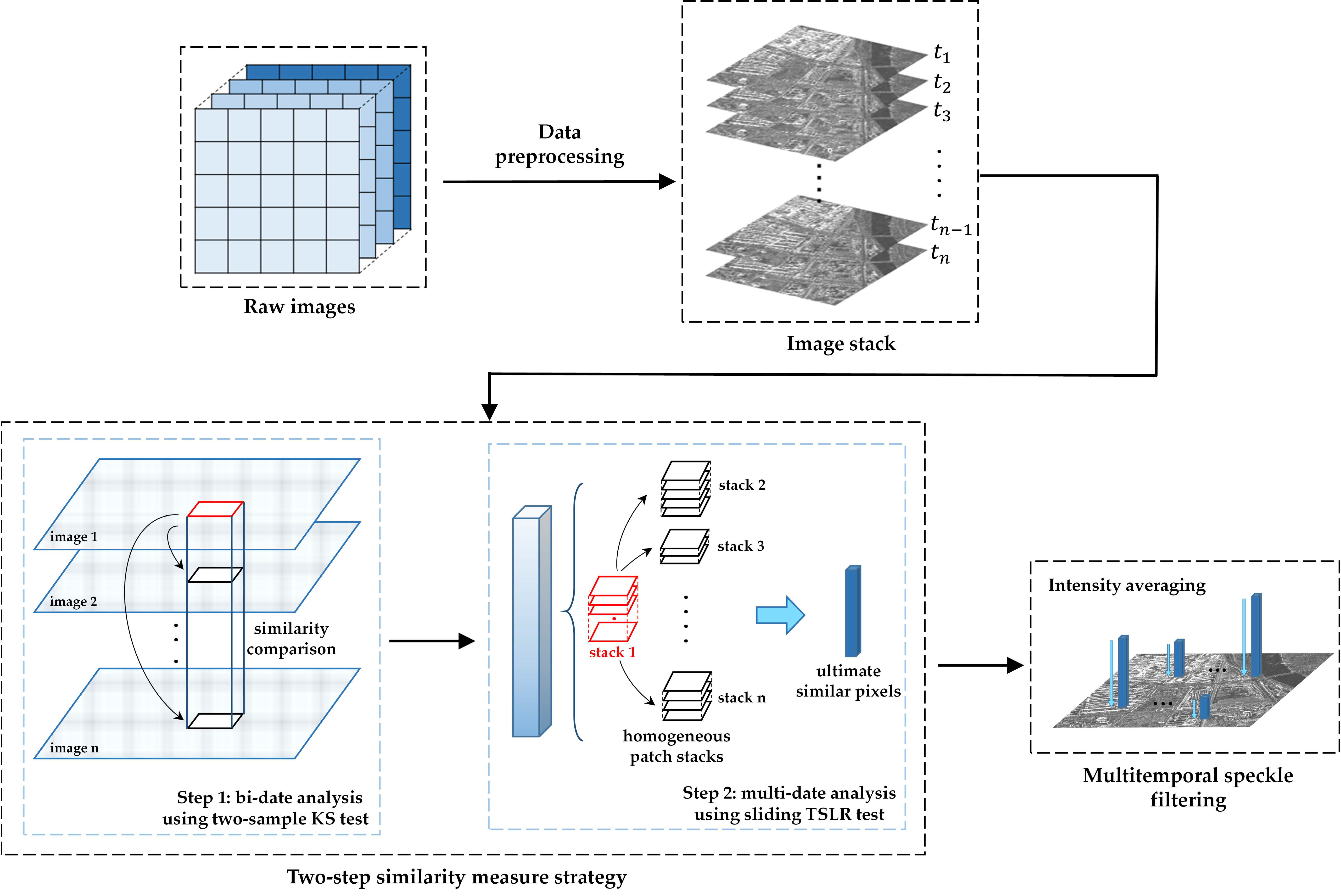
In order to make use of the 3-D data structure and enhance the performance of filtering results, we use a framework of a two-step filtering strategy. A different method is employed according to the data form at the first and second step, respectively. The workflow of the overall algorithm is depicted in Figure 1, which illustrates the procedure and the role of each part in the proposed multitemporal filtering method.

2.1. Data Preprocessing

For the purpose of achieving multitemporal speckle reduction, some basic SAR image preprocessing operations should first be carried out to avoid errors as much as possible, which mainly includes radiometric calibration and co-registration. First, because of the imaging peculiarity of the SAR data, such as radiation distortion, it should be calibrated radiometrically [35] in order to eliminate the difference between the observed value by sensors and the radiance of targets, so that the values of the pixels can represent the real backscatter strength of the terrestrial surface. Calibration is important for the quantitative application of SAR images. Then, co-registration is another fundamental procedure for multitemporal filtering and change detection, which aims to ensure that the position of the same ground objects within images taken at different times is identical. Wrong registration will not only lead to a serious impact on the filtering result, but also a lot of pseudo change points, so the registration precision usually demanded is a sub-pixel level [36]. In this paper, we use the GAMMA [37] software developed by Charles Werner and Urs Wegmüller in Gümligen, Switzerland to realize the radiometric calibration and co-registration of SAR images.

2.2. Two-Step Similarity Measure Strategy

In this section, a two-step strategy [32] is adopted for optimizing the process of detection for similar points, and a specific similarity measure algorithm is applied to corresponding steps according to the analysis of the data structure. Lastly, the filtered image is obtained by using the results from a previous similarity comparison.

2.2.1. Framework of the Two-Step Strategy

Given n SAR images collection $I=\left\{I_j;1\le j\le n\right\}$ which is co-registered in advance, j is the time position in the sequence where the image is located and relates to the data acquisition time. Let $I_j\left(x,y\right)$ be the pixel value located at the coordinate $\left(x,y\right)$ in the jth image $I_j$, and let $I_j^w\left(x,y\right)$ be the sliding boxcar window surrounding the central point, where $w$ denotes the window size. Then, we can get a pixel vector $\left\{I_j\left(x,y\right);1\le j\le n\right\}$ and a set of patches $\left\{I_j^w\left(x,y\right);1\le j\le n\right\}$ that are extended according to the time dimension. With that, a two-step similarity analysis approach is used to enhance the filtering performance in consideration of the collection of images.

• Step 1—Bi-date analysis

The similar patch extraction, which means finding unchanged pixels in the pixel vector, is conducted by a pairwise similarity comparison. Let us assume that M is the method that measures the similarity between any two dates, for example, j, k in the patch stack; then, the similarity degree can be obtained by

$$S_{j,k}^w\left(x,y\right)=M\left(I_j^w\left(x,y\right),I_k^w\left(x,y\right)\right),1\le j,k\le n.$$

(1)

Thus, for n-length time-series SAR images, the similar degree at the position (x, y) can be constructed as a two-dimension matrix with the size of n × n in accordance with the time order, which is called the similarity measure matrix and described as follows

$$S^w{\left(x,y\right)}_{n\times n}=\left(\begin{array}{cccc}{S}_{1,1}^w\left(x,y\right)& S_{1,2}^w\left(x,y\right)& \cdots & S_{1,n}^w\left(x,y\right)\\ S_{2,1}^w\left(x,y\right)& S_{2,2}^w\left(x,y\right)& \cdots & S_{2,n}^w\left(x,y\right)\\ \cdots & \cdots & \ddots & \cdots \\ S_{n,1}^w\left(x,y\right)& S_{n,2}^w\left(x,y\right)& \cdots & S_{n,n}^w\left(x,y\right)\end{array}\right),$$

(2)

where whether the matrix $S^w{\left(x,y\right)}_{n\times n}$ is symmetrical depends on the measure method. To distinguish the unchanged pixels from the changed ones in the pixel pile, a threshold $\lambda$ needs to be introduced. Given the threshold, the similarity measure matrix will be transformed into a binary matrix that only contains the value of 0 and 1.

$$D_{j,k}^w\left(x,y\right)=\{\begin{array}{c}0,S_{j,k}^w\left(x,y\right)\le \lambda \\ 1,S_{j,k}^w\left(x,y\right)>\lambda \end{array},1\le j,k\le n,$$

(3)

where 0 indicates that there are no significant changes between $I_j^w\left(x,y\right)$ and $I_k^w\left(x,y\right)$, and on the contrary, the pixel at time j is dissimilar to the one at time k if the result is equal to 1.

• Step 2—Multi-date analysis

After above bi-date analysis, we can obtain a collection $\Phi \left(I_j^w\left(x,y\right)\right)$ including all the similar patches of $I_j^w\left(x,y\right)$. In order to obtain pixels with a higher similarity precisely, this step substitutes the set $\Phi \left(I_j^w\left(x,y\right)\right)$ constructed by temporal neighborhoods for the previous patch form as the comparative object. Hence, the similarity degree between two sets is

$${\widehat{S}}_{j,k}^w\left(x,y\right)=M^{\prime }\left(\Phi \left(I_j^w\left(x,y\right)\right),\Phi \left(I_k^w\left(x,y\right)\right)\right),1\le j,k\le n,$$

(4)

and by comparing it with the threshold ${\lambda }^{\prime }$, the new similarity measure matrix is as follows

$${\widehat{D}}_{j,k}^w\left(x,y\right)=\{\begin{array}{c}0,{\widehat{S}}_{j,\mathrm{k}}^w\left(x,y\right)\le {\lambda }^{\prime }\\ 1,{\widehat{S}}_{j,\mathrm{k}}^w\left(x,y\right)>{\lambda }^{\prime }\end{array},1\le j,k\le n.$$

(5)

In this step, the main goal is to improve the result of step 1 by utilizing the information of multi-date neighborhoods. The matrix has the same pattern as that in step 1, and the greatest difference between the two steps is the similarity measurement method.

2.2.2. Two-Sample Kolmogorov-Smirnov Test for Homogeneous Patch Extraction

The Kolmogorov-Smirnov (KS) test is a form of hypothesis testing that inspects the equality of the distribution of the dataset. It has two forms of test for specific applications, which are respectively named as the one-sample KS test and two-sample KS test. The former is usually applied to the comparison between the sample and a proper reference probability distribution as a goodness-of-fit testing approach, and the latter is used to determine if the distributions of two sample data are significantly different. Here, we exploit the two-sample KS test as the similarity measurement approach in step 1, which is denoted by M in Equation (1). For the two-sample case, the test statistic is defined as

$$D_{KS}=\underset{-\infty <x<\infty }{\sup }\left|F_{1,l_1}\left(x\right)-F_{2,l_2}\left(x\right)\right|,$$

(6)

where $F_{1,l_1}\left(x\right)$ and $F_{2,l_2}\left(x\right)$ represent the empirical distribution functions of scattering intensity in two SAR patches, respectively; $l_1,l_2$ are the pixel number of a patch related to the window size; and sup denotes the supremum function.

The KS statistic takes the maximum distance between the empirical distribution functions as a measure of dissimilarity, and the null hypothesis (H₀) can be described as follows: the two patches located at the same position while acquired at different dates are statistically homogenous. (H₀) is accepted at the significant level α if

$$D_{KS}\le \sqrt{-\frac{1}{2}\ln \left(\frac{\alpha }{2}\right)}\sqrt{\frac{l_1+l_2}{l_1{l}_2}}.$$

(7)

In other words, the two patches are similar when the test statistic does not exceed the critical value. Equation (7) plays the role of finding out the homogenous patch and the right side of it is equivalent to the adaptive threshold λ in (3). Therefore, Equation (3) can be rewritten as

$$D_{j,k}^w\left(x,y\right)=\{\begin{array}{c}0,S_{j,\mathrm{k}}^w\left(x,y\right)\le \sqrt{-\frac{1}{2}\ln \left(\frac{\alpha }{2}\right)}\sqrt{\frac{l_1+l_2}{l_1{l}_2}}\iff I_k^w\left(x,y\right)\in \Phi \left(I_j^w\left(x,y\right)\right)\\ 1,S_{j,\mathrm{k}}^w\left(x,y\right)>\sqrt{-\frac{1}{2}\ln \left(\frac{\alpha }{2}\right)}\sqrt{\frac{l_1+l_2}{l_1{l}_2}}\iff I_k^w\left(x,y\right)\notin \Phi \left(I_j^w\left(x,y\right)\right)\end{array},1\le j,k\le n,$$

(8)

where $\Phi \left(I_j^w\left(x,y\right)\right)$ denotes the jth patch stack that is constructed by the patches similar to $I_j^w\left(x,y\right)$, and after the KS test, we can obtain n patch stacks that are the inputs for the STSLR test.

2.2.3. Sliding Time-Series Likelihood Ratio Test for Similarity Analysis of Patch Stacks

It has been previously mentioned that a collection of homogeneous patches is built with the bi-date analysis using a two-sample KS test; more precisely, the patch stack is generated at each date in the same spatial coordinate, which means n patch stacks for n-length images. However, the two-sample KS test is not suitable for the multi-date analysis in step 2 of the two-step similarity measure framework due to the element form of the patch stack, which will decrease the accuracy and reliability of the ultimate similar pixels. Therefore, a novel method called the STSLR test is proposed to analyze the similarity between any two patch stacks and to refine the results from the last step, which is appropriate for the processing of a three-order tensor. The idea is inspired by the joint-scatterer interferometric SAR (JSInSAR) technology [38], where the similarity between two JS tensors located at different positions is judged by the time-series likelihood ratio (TSLR) test.

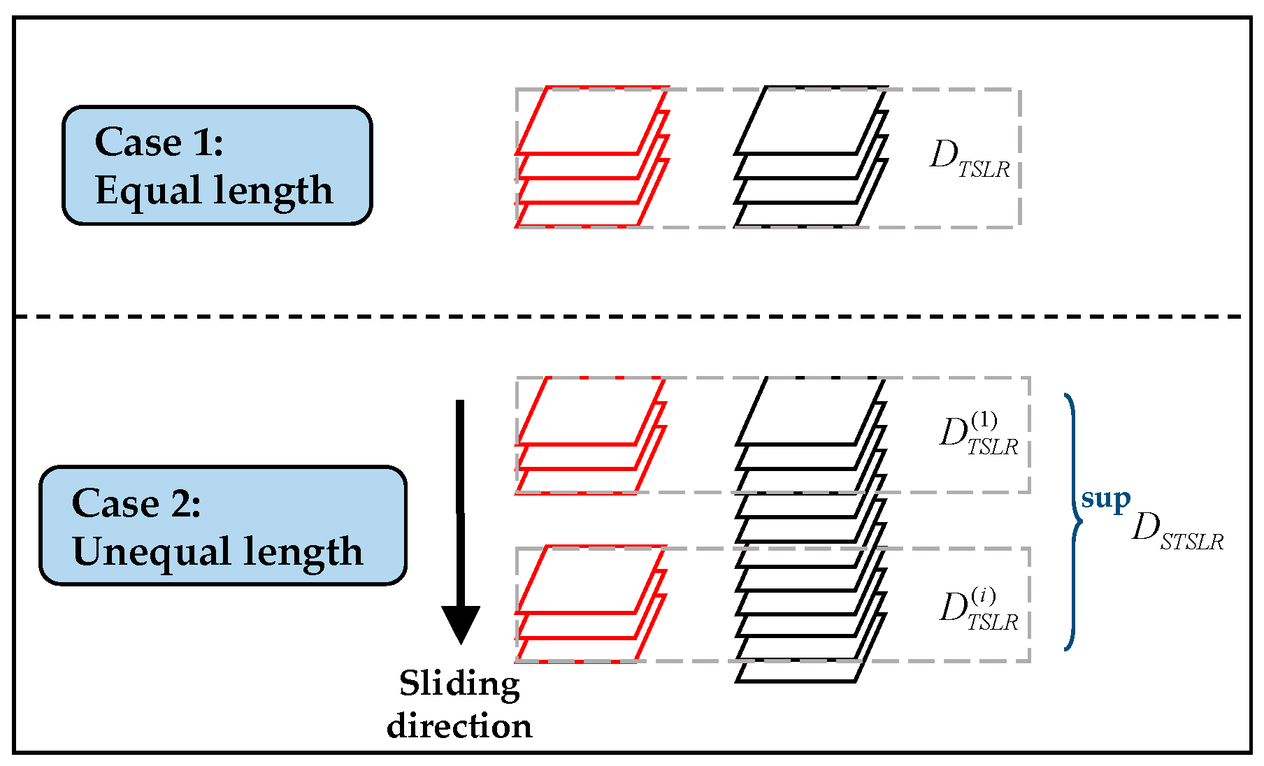
As shown in Figure 2, there are two cases in the process of multitemporal analysis. In the first case, two comparative patch stacks have the same length, and each stack can be represented by

$$P\left(\ell \right)=\left[{\mathit{x}}_1\left(\ell \right),{\mathit{x}}_2\left(\ell \right),\dots ,{\mathit{x}}_m\left(\ell \right)\right],$$

(9)

which is a three-order tensor that consists of m patches, where ${\mathit{x}}_i\left(\ell \right)$ is the $i$-th patch centered at the $\ell$-th pixel, and m is the length of a patch stack obtained from the KS test. Before evaluating whether two equal-length patch stacks are statistically homogeneous, a measurement criterion between the pair of patches that can be extended to a higher dimension should first be established. Considering two patches in the same order denoted by ${\mathit{x}}_{1,i}$ and ${\mathit{x}}_{2,i}$, respectively, the pair $\left({\mathit{x}}_{1,i},{\mathit{x}}_{2,i}\right)$ is similar when they are generated from the probability distribution function (PDF) with uniform parameters, which can be interpreted as hypothesis testing given by

$$\begin{array}{l}{\mathcal{H}}_0:{\theta }_1={\theta }_2\equiv {\theta }_{12},\\ {\mathcal{H}}_1:{\theta }_1\ne {\theta }_2,\end{array}$$

(10)

where ${\theta }_i$ is the parameter of PDF and $1\le i\le m$. Based on the Neyman-Pearson lemma [39], the likelihood ratio test statistic is the optimal criterion for the measurement:

$${\Lambda }^{(i)}\left({\mathit{x}}_{1,i},{\mathit{x}}_{2,i}\right)=\frac{L\left({\theta }_{12}|{\mathit{x}}_{1,i},{\mathit{x}}_{2,i};{\mathcal{H}}_0\right)}{L\left({\theta }_1,{\theta }_2|{\mathit{x}}_{1,i},{\mathit{x}}_{2,i};{\mathcal{H}}_1\right)}$$

(11)

where the similarity degree between ${\mathit{x}}_{1,i}$ and ${\mathit{x}}_{2,i}$ is proportional to the value of $\Lambda \left({\mathit{x}}_{1,i},{\mathit{x}}_{2,i}\right)$. Drawing on the experience from the two-sample KS test, the definition of the TSLR test statistic [38] is as follows

$$D_{TSLR}=\sup \left|-2\log {\Lambda }^{(i)}\left({\mathit{x}}_{1,i},{\mathit{x}}_{2,i}\right)\right|,$$

(12)

where $-2\log {\Lambda }^{(i)}$ represents i.i.d. random variables, and the $D_{TSLR}$ is the supremum of the absolute value of the likelihood ratio test statistics $-2\log {\Lambda }^{(i)}\left({\mathit{x}}_{1,i},{\mathit{x}}_{2,i}\right)$, where each ${\Lambda }^{(i)}\left({\mathit{x}}_{1,i},{\mathit{x}}_{2,i}\right)$ represents the similarity between a pair of patches.

Generally, the parameter ${\theta }_i$ of a PDF is unavailable, i.e., the hypothesis is not simple. In these situations, we usually use the estimated parameters obtained by the maximum likelihood estimation (MLE) method, which is called the GLR test. Considering that the research site in the experimental data is mainly an urban area and contains a rich variety of ground features, we use the lognormal distribution as the PDF of the likelihood function, which is a good statistical representation of clutter in the case of heterogeneous terrain.

We assume that the amplitudes of scatterers in two patches $\left({\mathit{x}}_{1,i},{\mathit{x}}_{2,i}\right)$ follow a lognormal distribution with parameters $\left(\mu ,\eta \right)$, i.e., $x_{1i,l}~f_L\left(x;{\mu }_{1,i},{\eta }_{1,i}\right)$ and $x_{2i,l}~f_L\left(x;{\mu }_{2,i},{\eta }_{2,i}\right)$, $l=1,\dots ,w_0$, where $w_0$ is the number of scatterers in each patch. Under ${\mathcal{H}}_0$, the hypothesis test can be redescribed as: ${\eta }_{1,i}^2={\eta }_{2,i}^2={\eta }_{12,i}^2$. According to the MLE method, the estimated value of ${\eta }_{12,i}^2$ is as follows

$${\widehat{\eta }}_{12,i}^2=\frac{{\widehat{\eta }}_{1,i}^2+{\widehat{\eta }}_{2,i}^2}{2},$$

(13)

where ${\widehat{\eta }}_{1,i}^2$ and ${\widehat{\eta }}_{2,i}^2$ are the MLEs of parameters ${\eta }_{1,i}^2$ and ${\eta }_{2,i}^2$, respectively. Therefore, the GLR becomes

$${\Lambda }^{(i)}\left({\mathit{x}}_{1,i},{\mathit{x}}_{2,i}\right)=\frac{{\left({\widehat{\eta }}_{1,i}^2\right)}^{\frac{w_0}{2}}{\left({\widehat{\eta }}_{2,i}^2\right)}^{\frac{w_0}{2}}}{{\left({\widehat{\eta }}_{12,i}^2\right)}^{w_0}}.$$

(14)

Finally, the modified $D_{TSLR}$ is given by

$$D_{TSLR}=\sup \left|-2\log \left(\frac{{\left({\widehat{\eta }}_{1,i}^2\right)}^{\frac{w_0}{2}}{\left({\widehat{\eta }}_{2,i}^2\right)}^{\frac{w_0}{2}}}{{\left({\widehat{\eta }}_{12,i}^2\right)}^{w_0}}\right)\right|.$$

(15)

According to the Wilks’s theorem [40], the null distribution of $-2\log {\Lambda }^{(i)}$ trends towards a chi-square distribution with degrees of freedom equal to $d$ as the sample size approaches infinity, so the cumulative distribution function (CDF) of $D_{TSLR}$ can be derived as follows

$$\begin{array}{ll}F\left(D_{TLSR}\le t\right)& =F\left(-2\log {\Lambda }^{(1)}\le t,-2\log {\Lambda }^{(2)}\le t,\dots ,-2\log {\Lambda }^{(m)}\le t\right)\\ & =F_{{\chi }^2}{\left(t;d\right)}^m,\end{array}$$

(16)

where $m$ denotes the length of the patch stack, and the PDF is just the derivative of the CDF. Thus, the null hypothesis that two patch stacks $P_1\left(\ell \right)$ and $P_2\left(\ell \right)$ are considered to be similar is accepted if $D_{TLSR}\le C$, where $C$ is the threshold determined by the equation $F\left(D_{TLSR}\le C\right)=1-\alpha$.

Nevertheless, the length between two patch stacks is different in most situations, where the TSLR test is no longer applicable. As a result, the sliding TSLR is proposed for the second case. Given two stacks $h_1$ and $h_2$, we use the shorter stack $h_1$ as the sliding object. Then, the problem will be transformed into an integration of case 1 by comparing $h_1$ with the same length part in the longer stack $h_2$, and the test statistic of STSLR is written as

$$D_{STSLR}=\sup \left|D_{TLSR}^{(i)}\right|,0\le i\le \left(h_2-h_1+1\right),$$

(17)

where each $D_{TSLR}^{(i)}$ represents the similarity between equal length stacks, and the STSLR test statistic is the maximum TSLR statistic. The distribution of $D_{STSLR}$ is identical to the TSLR test statistic and the threshold $C$ can be used to distinguish between the dissimilarity and similarity.

2.3. Multitemporal Speckle Filtering

After two-step similarity measurement, the pixels with a high similarity can be found in time-series more accurately. The filtering procedure depends on the result of multi-date analysis, which includes the information of unchanged pixels for every point. To obtain the final filtered images, we use the statistical mean to deal with the similar pixels

$${\widehat{I}}_j\left(x,y\right)=\frac{1}{N_{{\Phi }_j\left(x,y\right)}}{\displaystyle \sum _{k=1}^{N_{{\Phi }_j\left(x,y\right)}}\left(1-{\widehat{D}}_{j,k}^w\left(x,y\right)\right)}{I}_k\left(x,y\right),$$

(18)

where $N_{{\Phi }_j\left(x,y\right)}$ is the number of elements contained in the collection $\Phi \left(I_j^w\left(x,y\right)\right)$.

3. Experiments and Results

In this section, the proposed algorithm will be compared with the other four speckle filtering methods in order to evaluate its feasibility and effectiveness, two of which are classical multitemporal filtering methods Quegan’s filter (QF) [31] and change detection matrix based filter (CDMF) [32], and the remaining two are the state-of-the-art in single-temporal and multi-temporal speckle filtering approaches called fast adaptive nonlocal SAR despeckling (FANS) [41] and multitemporal SAR block-matching and 3D filtering (MSAR_BM3D) [34], respectively. Due to the lack of a noise-free reference image, the performance assessment in SAR image despeckling usually depends on the original or filtered images. To evaluate the performance of each method more comprehensively and accurately, we carried out the experiments on real multitemporal SAR images and synthetic SAR images by using the above approaches. The optimal parameters of each experiment were obtained by the trial-and-error method. The setting of parameters in each method is as follows: (i) the local window size of QF was set as 3 × 3; (ii) in the CDMF approach, the window size was 3 × 3 and $\eta =0.95$; (iii) the parameters of the FANS and MSAR_BM3D were set as suggested in the reference paper; and (iv) the parameters of the proposed method were set to ${\alpha }_{KS}=0.05$ and ${\alpha }_{STSLR}=0.05$, where the window size was 3 × 3.

3.1. Comparsion on Synthetic Multitemporal Synthetic Aperture Radar Images

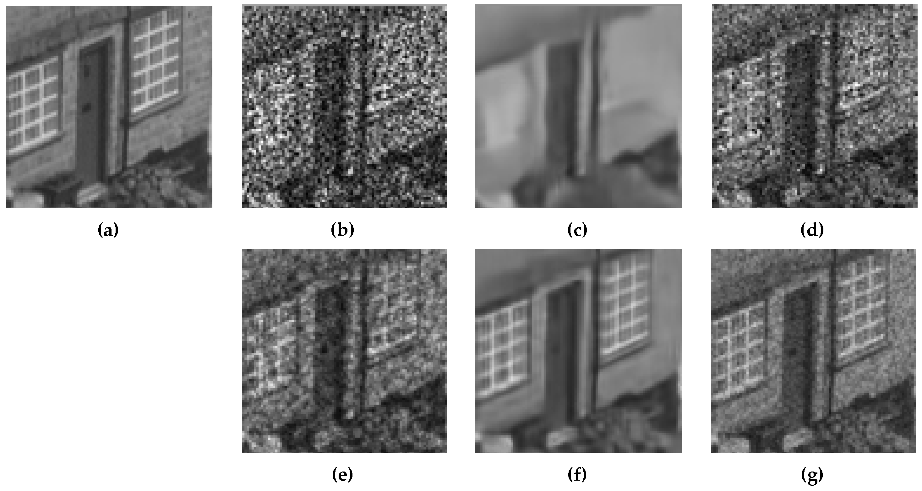
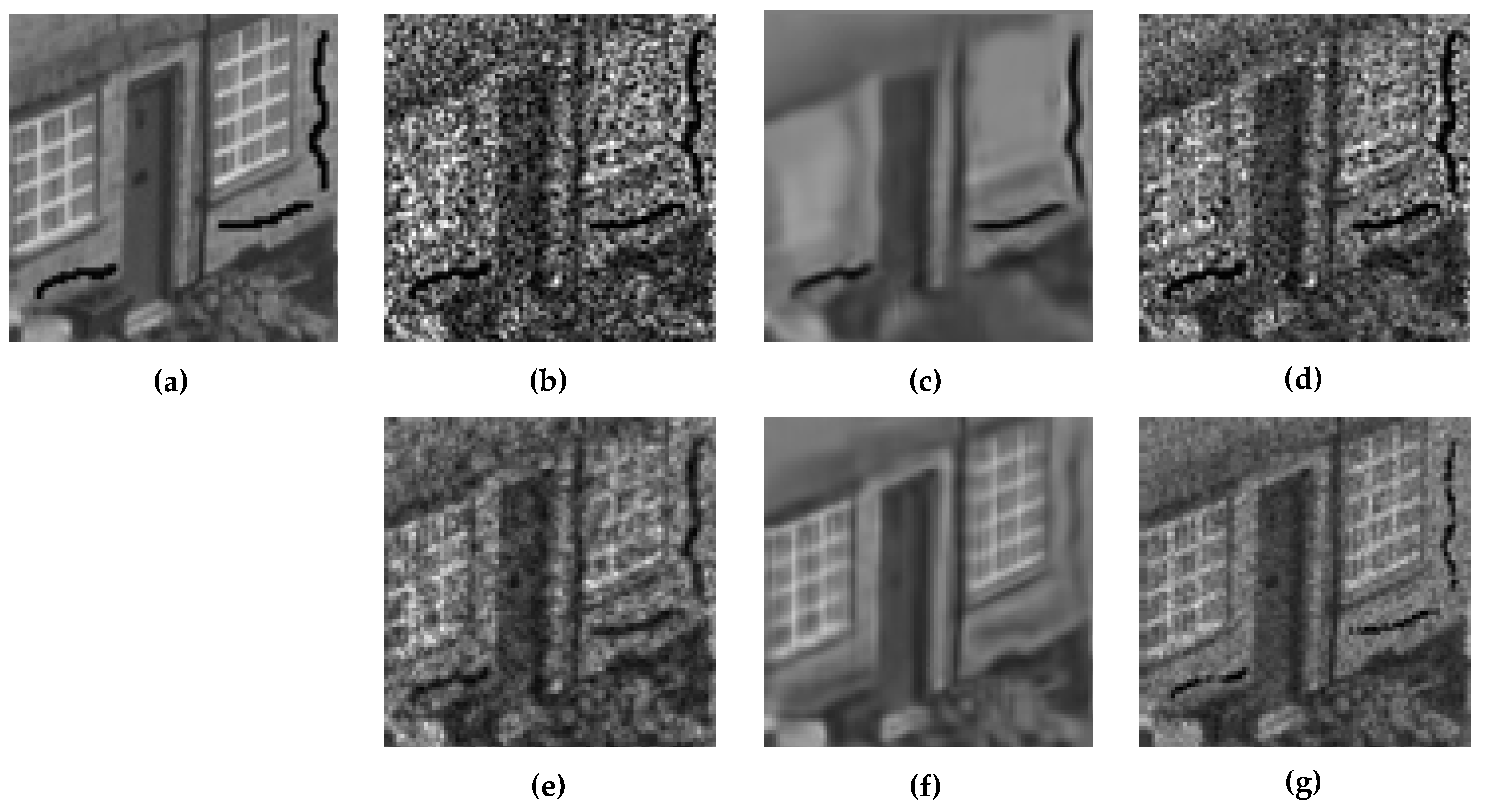
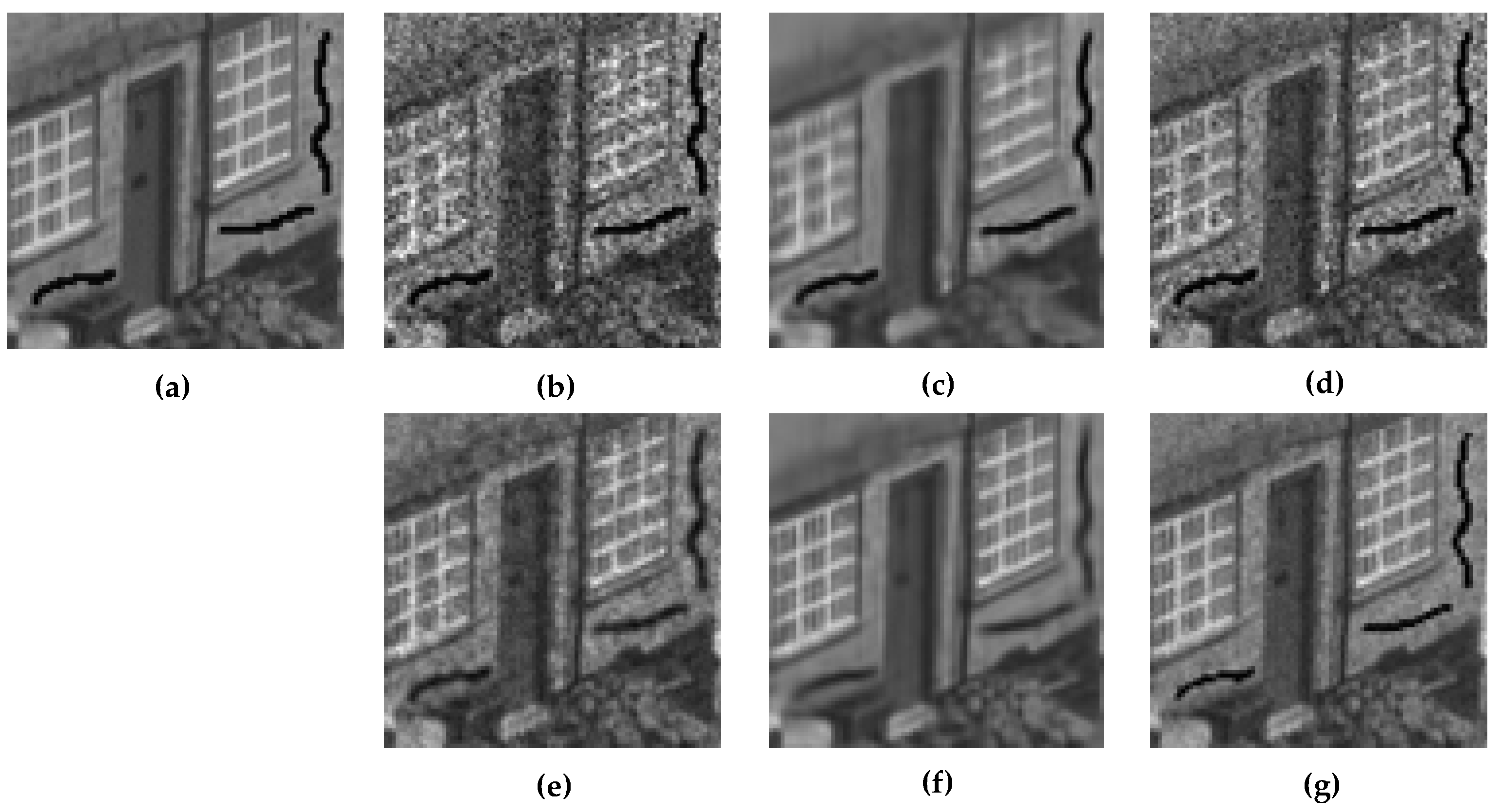
In this simulated experiments, the synthetic multitemporal images are generated by multiplying the optical images with simulated speckle noise, and the noise obeys the Rayleigh distribution [42]. To evaluate the quantitative performance of each method, we adopted the indices of peak signal-to-noise ratio (PSNR) and structural similarity (SSIM) to measure the degree of similarity between the distorted image and reference image. Firstly, we generated two sets of eight SAR-like images with 1-Look speckle noise to simulate time-series SAR images. The first set of images did not change over time. Considering that the simulation of temporal change helps to better analyze the effects of each approach, we added three dark lines to the first image of the second set. In addition, we added eight images to evaluate the impact of the increased number of images on the simulation results. Finally, we added a group of experiments based on 4-Looks speckle noise to assess the performance of different approaches from multi-aspects. The filtering results of the local region of two sets with eight images and 1-Look speckle are shown in Figure 3 and Figure 4. The 4-Looks results are shown in Figure 5 and Figure 6.

Table 1. The quantitative results of different methods on synthetic aperture radar (SAR) images (peak signal-to-noise ratio (PSNR) and structural similarity (SSIM), PSNR-SSIM).

Image Number	Noisy (1-Look)	FANS	CDMF	QF	MSAR_BM 3D	Proposed
8 (unchange)	14.07–0.240	22.51–0.517	17.01–0.397	19.50–0.554	28.07–0.845	21.35–0.658
8 (change)	14.21–0.299	22.09–0.563	16.63–0.446	19.33–0.599	23.26–0.774	20.72–0.680
16 (unchange)	14.07–0.240	22.51–0.517	18.58–0.508	20.37–0.612	29.57–0.887	24.46–0.757
16 (change)	14.21–0.299	22.09–0.563	18.02–0.522	19.99–0.654	23.82–0.817	22.33–0.768

and

Table 2. The quantitative results of different methods on synthetic SAR images (PSNR-SSIM).

Image Number	Noisy (4-Looks)	FANS	CDMF	QF	MSAR_BM3D	Proposed
8 (unchange)	19.41–0.504	26.52–0.791	22.89–0.678	25.74–0.802	31.78–0.924	28.24–0.857
8 (change)	19.54–0.573	26.07–0.830	22.21–0.719	24.69–0.827	26.94–0.905	26.62–0.878
16 (unchange)	19.41–0.504	26.52–0.791	24.98–0.764	26.91–0.841	33.45–0.946	31.10–0.915
16 (change)	19.54–0.573	26.07–0.830	23.69–0.795	25.32–0.857	26.74–0.912	27.84–0.917

present the quantitative results based on a different number of looks of speckle noise, respectively.

From Table 1, we can see that the proposed method and MSAR_BM3D achieved the best results in the four groups of experiments. Take the unchanged case as an example. Since FANS is based on a single image, its indexes remain unchanged with the increase in the number of images, while the proposed method gains up to 3.11 dB and 0.099 on PSNR and SSIM, respectively, which indicates that the exploitation of temporal information helps improve the filtering effect. Then, we can compare the results of the first two sets in the table, and it can be observed that the PSNR of MSAR_BM3D drops dramatically when introducing the temporal change, close to 5 dB. This is mainly because the three dark lines added were smoothed out too much (see Figure 4f), resulting in the large difference between the filtered and reference image. However, the proposed method retains most of the temporal change, and the PSNR only decreased by 0.63 dB.

As for the case of 4-Looks speckle noise, it can be seen that the results shown in Figure 5 and Figure 6 are much better than those of Figure 3 and Figure 4, both in terms of quantitative indices and qualitative filtering effects due to noise reduction. Table 2 shows that the proposed method is better than the single-temporal method of FANS because of the exploitation of temporal information, and the denoising effect can be further improved with the increase of the number of images. In addition, the proposed method is more effective than MSAR_BM3D in the use of temporal information, and our method achieves the best performance in the changing case with 16 images.

3.2. Comparison on Real Multitemporal Synthetic Aperture Radar Images

3.2.1. Data Description

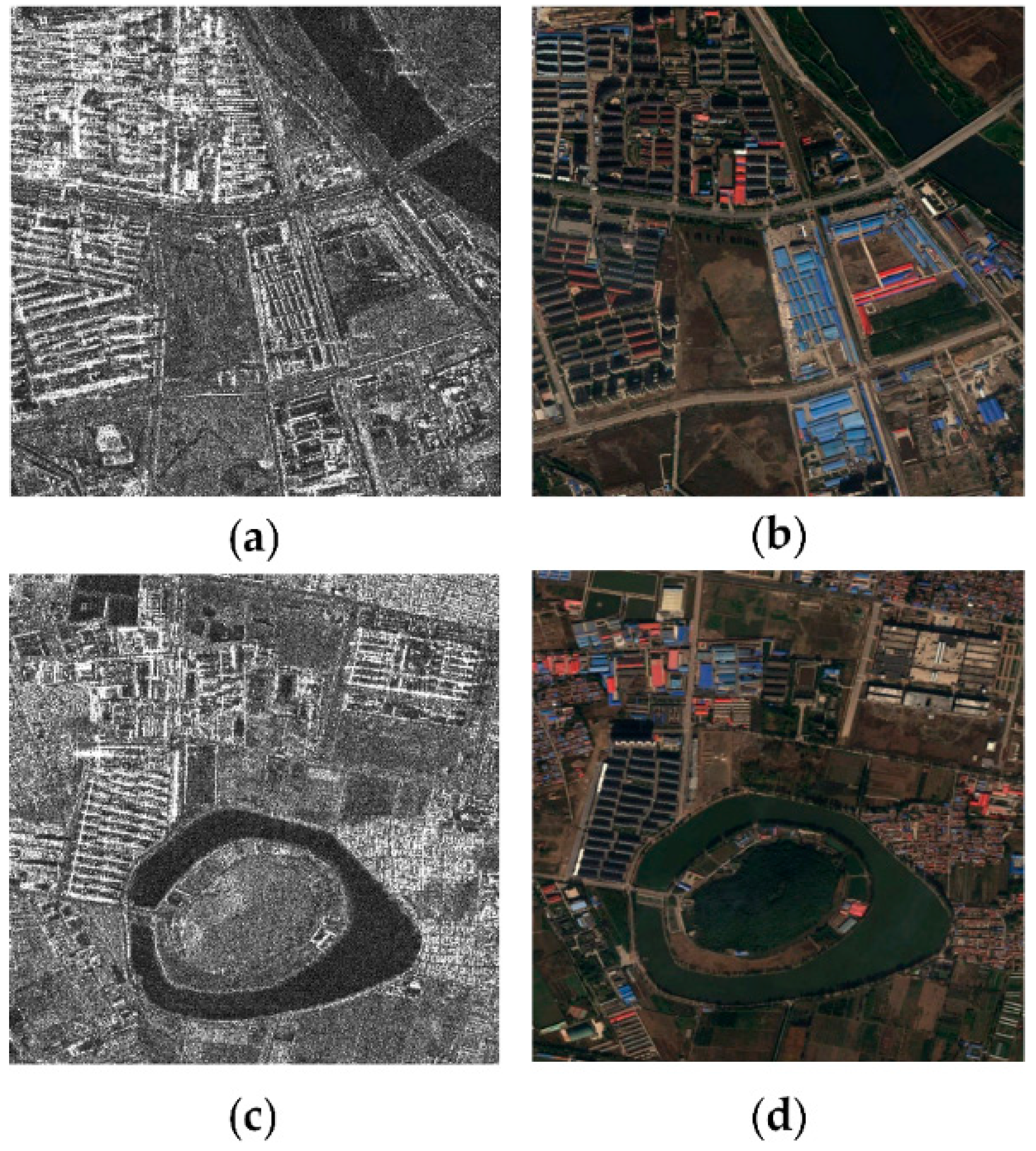
To assess the performance of the proposed method more accurately, two datasets of real SAR images acquired by TerraSAR-X from Tongzhou District of Beijing, China, are used as the experimental data. TerraSAR-X is a commercial SAR satellite operating in the X-band and launched in 2007, with a revisit period of 11 days. The highest spatial resolution of the spotlight and strip imaging modes is 1 and 3 m, respectively, and these modes are commonly used in earth observation tasks. As the sub-center of Beijing, Tongzhou District bears the future development of the capital and has been undergoing rapid changes in recent years. The complicated land cover changes in the demolition and reconstruction of urban buildings are conducive to verify the reliability and robustness of the similarity measurement in this paper. The first dataset consists of 13 single-look complex SAR images acquired from 22 January 2012 to 8 March 2016 with a size of 1000 × 1000 and a 2-m resolution, and the features included in this dataset are mainly residential areas, bridges, and rivers. The first SAR image of the time-series and the corresponding optical image are shown in Figure 7a,b. The second dataset has the same size and resolution as the first one, which contains 12 images acquired between 28 March 2012 and 8 March 2016. It covers a lake island, factory buildings, crops, etc. Figure 7c,d show the dataset and the optical image.

3.2.2. Experimental Results and Analysis

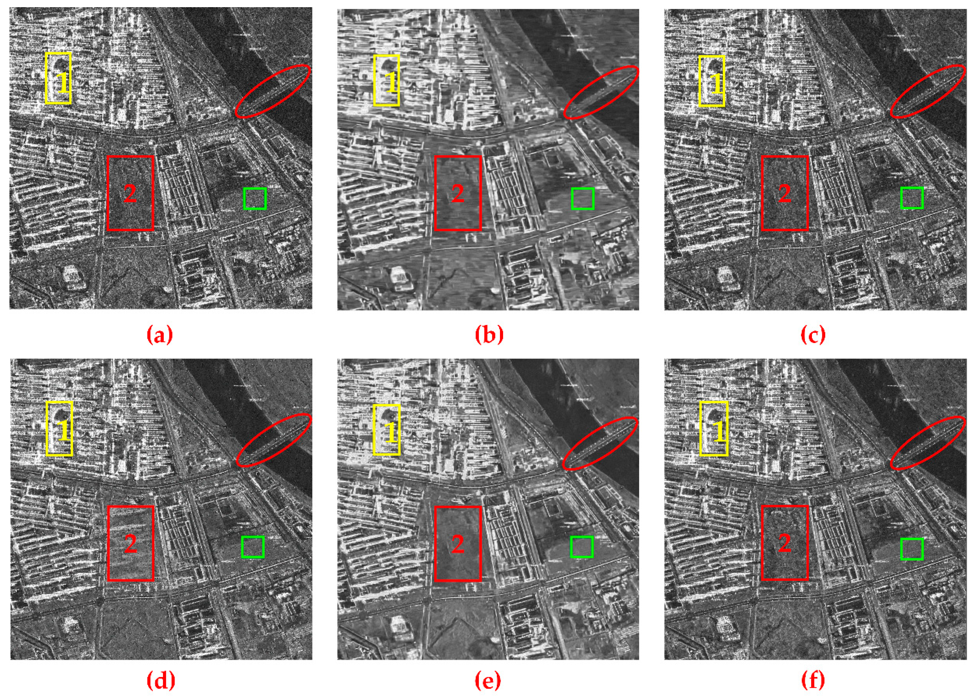
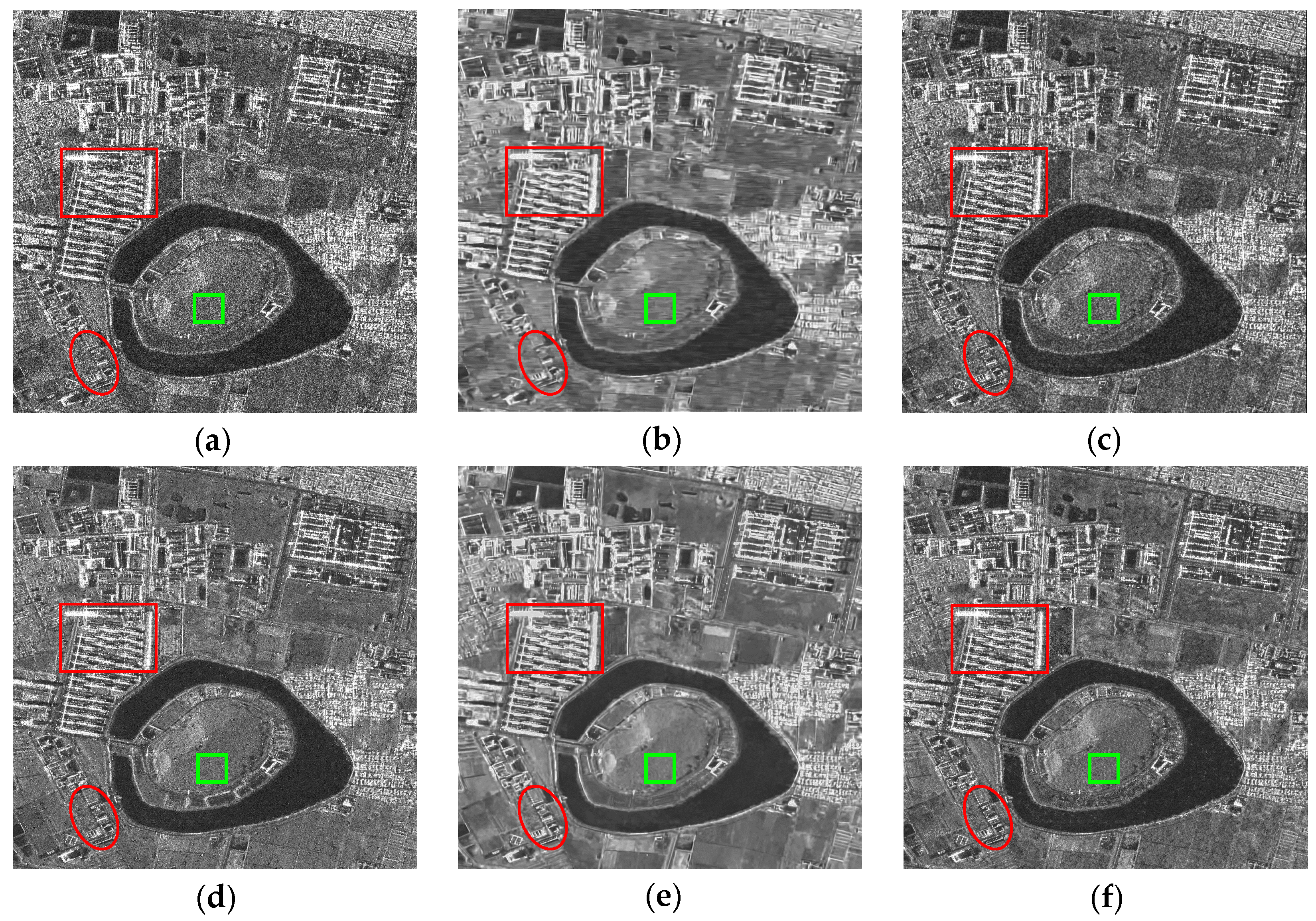
The speckle filtering results of Dataset 1 are depicted in Figure 8. Considering the length of the article, we cannot list the filtering results of SAR images at all times. Therefore, the experimental results of a representative image in the time-series are given as the analysis object. Figure 8a is the original SAR image acquired on 22 January 2012 from Dataset 1, which is seriously corrupted by the speckle noise. Figure 8b is the filtering result using the FANS method. Although there is a great enhancement of the suppression effect for the speckle, the details information of the image displays a great loss, which is the defect of the non-temporal filter. For instance, the red ellipse in the upper right corner of the figure contains a bridge, and the strong scattering points on both sides of the bridge are the street lamps. It can be seen from Figure 8b that the lamps are too blurred compared to the other multitemporal filtering approaches. Figure 8c shows the result of QF, where the smoothness for the noise is not obvious due to the change of the ground objects. Figure 8d gives the CDMF multitemporal filtering result, which has a smoother effect and better image detail preservation ability compared to the previous methods. However, there are some imaginary shadows of the buildings in red box 2 because of the error detection of similar points, which changes the surface feature information of the original image. Figure 8e presents the result of the MSAR_BM3D approach, for which we can see that the suppression effect of speckle noise is further improved, taking advantaging of the temporal and non-local information. However, the brightness of the image displays a certain decline and the building areas present are somewhat over-smoothed, which leads to a little unnaturalness, such as the residential buildings in yellow box 1. The proposed method is shown in Figure 8f, where the smoothing effect has been largely improved and the naturalness and details of the filtered image are well preserved because of the high precision for the detection of similar pixels in the temporal axis, which maintians a high degree of consistency with the original image.

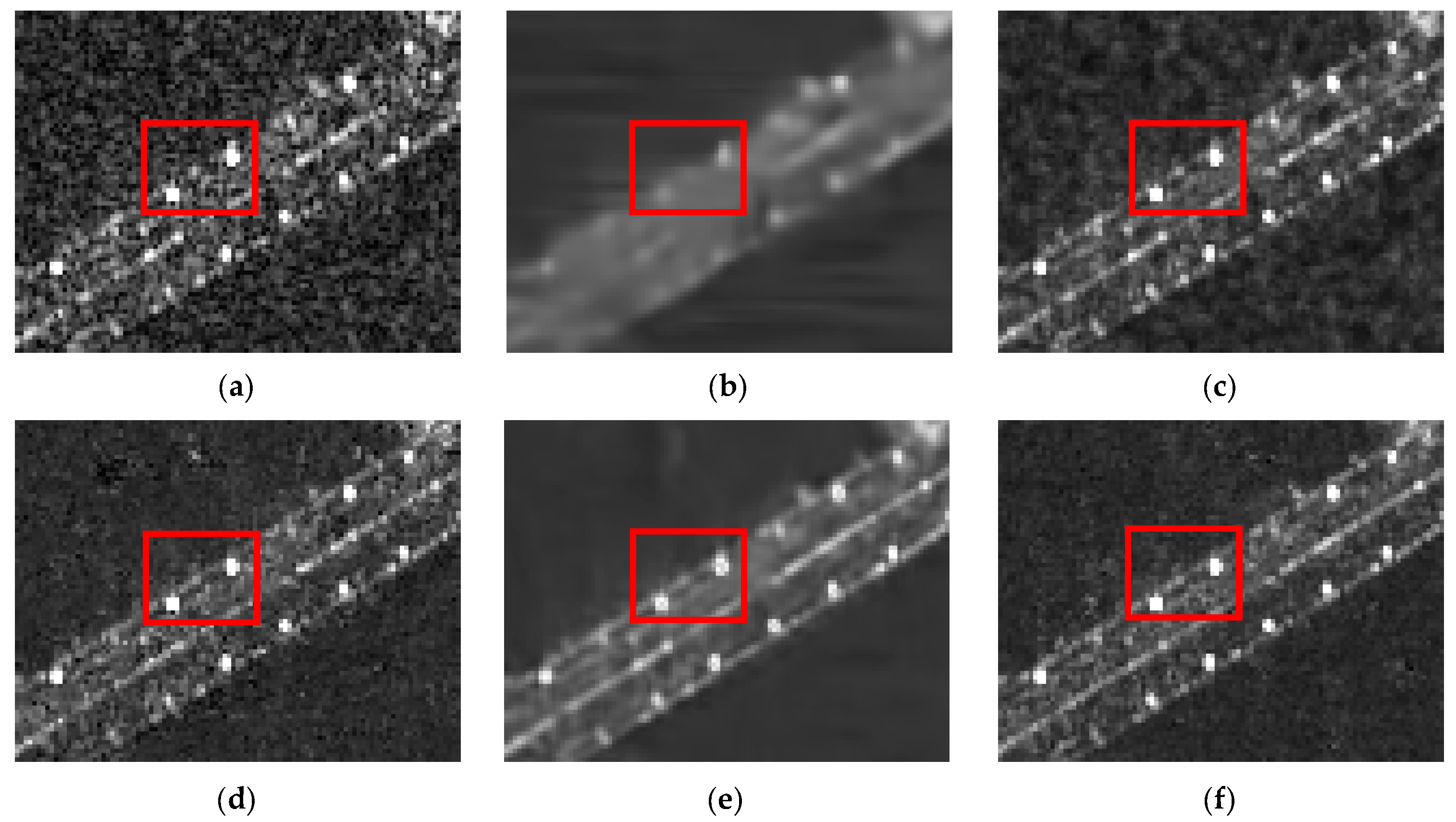
The preservation capability of strong point targets is an important qualitative evaluation index for measuring the performance of different filtering methods. In order to better compare the effect of each method in this ability, we cropped the bridge region within the ellipse in Figure 8 as the analytic object. It can be seen from Figure 9 that the filtering results of FANS and MSAR_BM3D have different degrees of ambiguity, while the other three approaches, including that proposed in this paper, show a better preservation ability for strong point targets.

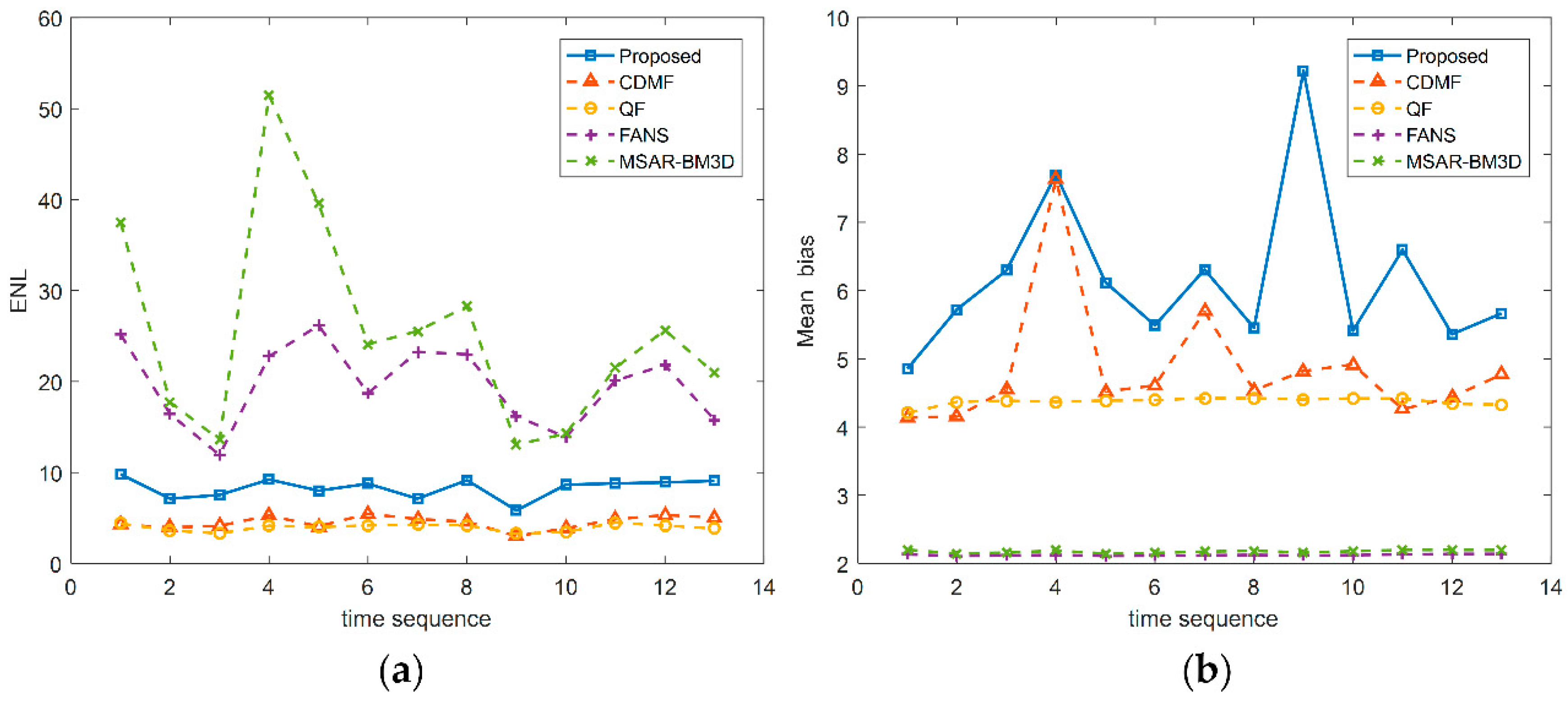
To further assess the experimental results of each method, we introduce two quantitative evaluation indices: the equivalent number of looks (ENL) and mean bias (MB). The ENL is used to measure the degree of speckle reduction, which is calculated as $ENL=\frac{{\mu }^2}{{\sigma }^2}$, where μ and σ represent the mean and standard deviation of a local homogeneous area, respectively, which is shown as a green square with about 50 × 50 pixels in Figure 8. Then, mean bias is expressed as $MB=\frac{{\mu }_{I_2}-{\mu }_{I_1}}{{\mu }_{I_1}}$, where ${\mu }_{I_1},{\mu }_{I_2}$ are the statistical mean of the whole image before and after the filtering operation. According to the product model and the statistical properties of speckle noise, the mean bias should be equal to 0 in the ideal case [20,42,43], so this index can characterize the information preservation ability of the filtering method to the feature of the ground object. The closer the value is to 0, the better the filter method maintains the average of the image, i.e., the less loss of image detail information. In order to better compare the difference of mean deviation for each method, a negative logarithm is applied, which is revised as $MB=-\log \left|\frac{{\mu }_{I_2}-{\mu }_{I_1}}{{\mu }_{I_1}}\right|$. Thus, the larger the MB, the better the retention of image information for the method.

The quantitative results of images at every time obtained by five different algorithms are listed in

Table 3. The quantitative comparison of different filtering results for Dataset 1, using equivalent number of looks (ENL).

No.	ENL
	Origin	FANS	CDMF	QF	MSAR_BM3D	Proposed
1	0.92	25.17	4.26	4.38	37.48	9.81
2	0.87	16.43	3.97	3.63	17.73	7.13
3	0.89	11.91	4.13	3.30	13.60	7.53
4	0.99	22.76	5.26	4.15	51.44	9.23
5	0.96	26.16	4.08	4.00	39.55	8.01
6	0.93	18.72	5.45	4.18	24.09	8.77
7	0.85	23.26	4.89	4.25	25.54	7.13
8	0.94	22.99	4.59	4.20	28.26	9.15
9	0.85	16.18	3.00	3.25	13.07	5.83
10	0.84	13.87	3.86	3.45	14.26	8.66
11	0.92	20.10	4.86	4.49	21.50	8.80
12	0.93	21.80	5.31	4.16	25.65	8.92
13	0.88	15.80	5.05	3.85	20.93	9.08
Mean	0.91	19.63	4.52	3.95	25.62	8.31

and representing ENL and MB, respectively. From Table 3, we can see that the higher ENL is achieved by the proposed method, FANS, and MSAR_BM3D. However, in

Table 4. The quantitative comparison of different filtering results for Dataset 1, using mean bias (MB).

No.	Mean Bias (MB)
	FANS	CDMF	QF	MSAR_BM3D	Proposed
1	2.1328	4.1384	4.2081	2.2018	4.8555
2	2.1115	4.1545	4.3679	2.1444	5.7248
3	2.1164	4.5465	4.3856	2.1586	6.2961
4	2.1245	7.6344	4.3708	2.1888	7.7011
5	2.1118	4.5191	4.3884	2.1449	6.1204
6	2.1135	4.6101	4.3931	2.1544	5.4897
7	2.1187	5.6915	4.4240	2.1743	6.3087
8	2.1257	4.5390	4.4226	2.1876	5.4535
9	2.1150	4.8211	4.4041	2.1601	9.2219
10	2.1229	4.9170	4.4199	2.1813	5.4119
11	2.1323	4.2597	4.4173	2.1984	6.5975
12	2.1392	4.4409	4.3403	2.2000	5.3605
13	2.1396	4.7689	4.3288	2.1972	5.6655
Mean	2.1234	4.8493	4.3747	2.1763	6.1698

. the mean biases of FANS and MSAR_BM3D are relatively worse than the other three algorithms due to the use of a non-local operation, which decreases the brightness and some details of images. Our method performs much better than QF and CDMF in mean bias because of the high accuracy of searching for similar points in the time dimension. Considering that the subsequent application of time-series SAR images is mainly in classification and change detection, the maintenance of temporal and detail information of images is more important. Therefore, the proposed method achieves better results.

Figure 10a,b intuitively show the variation trends of the filtering effect on all images for the proposed framework and another four methods. The horizontal axis indicates the change of the image acquisition time, and the different colored lines represent the results of different methods with time.

Figure 11 shows the filtering results of Dataset 2. The acquisition time of the representative image is 28 March 2012, which is the first scene in the time-series and shown in Figure 11a. Analogously, the isolated targets have been almost eliminated by FANS in the red elliptical area (see Figure 11b), whereas the other multitemporal algorithms still retain the information of those isolated objects. Figure 11c–e shows the results of QF, CDMF, and MSAR_BM3D, respectively. It can be seen that the speckle suppression effect of QF improves little; in the meantime, the results of CDMF for the factory buildings surrounding the vegetation in the lake island also display some erroneous traces of construction, and the MSAR_BM3D result shows some degradation of the image brightness and detail information within the red box, in spite of the high smoothness. The result of the proposed method is shown in Figure 11f, which presents a better comprehensive filtering effect than the other methods.

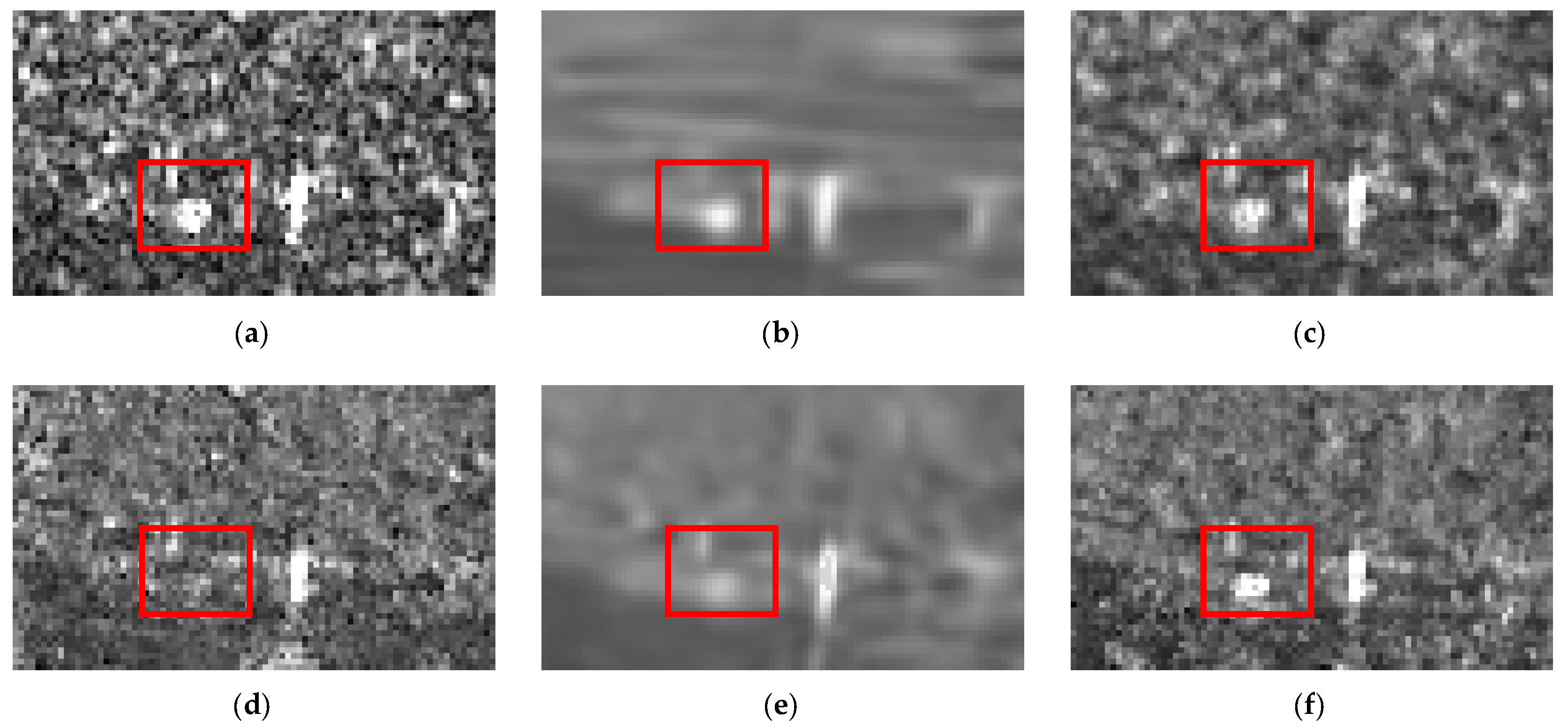
In order to analyze the ability of each method to preserve the point targets in Dataset 2, we selected a region that contains the strong point. It can be observed from Figure 12 that FANS and MSAR_BM3D have the problem of over-smoothing, which reduced the brightness of the point after filtering. CDMF failed to maintain the target and there was a slight loss in the result of QF, while the proposed method achieved the best preservation capability for strong point targets.

Table 5. The quantitative comparison of different filtering results for Dataset 2 (ENL).

No.	ENL
	Origin	FANS	CDMF	QF	MSAR_BM3D	Proposed
1	0.96	20.39	4.68	4.44	25.07	9.50
2	0.92	29.39	4.59	4.33	30.30	9.10
3	0.85	19.72	3.98	4.54	17.26	8.95
4	0.93	25.84	4.51	4.38	29.92	9.48
5	0.94	23.69	5.16	4.28	28.17	9.55
6	0.98	28.73	4.62	4.70	42.29	10.02
7	0.98	34.98	4.34	4.83	40.38	10.02
8	0.95	28.97	4.35	4.64	28.24	9.63
9	0.91	22.53	4.71	4.20	35.07	8.88
10	0.86	20.16	5.19	4.35	20.65	8.43
11	0.83	20.08	4.02	3.74	28.46	8.17
12	0.89	19.74	4.55	3.83	22.55	8.64
Mean	0.92	24.52	4.56	4.36	29.03	9.20

and

Table 6. The quantitative comparison of different filtering results for Dataset 2 (MB).

No.	Mean Bias (MB)
	FANS	CDMF	QF	MSAR_BM3D	Proposed
1	2.1144	4.9023	4.3143	2.1656	5.1611
2	2.1070	5.1058	4.3916	2.1392	5.8887
3	2.1035	4.0422	4.4278	2.1328	5.6099
4	2.1115	4.5933	4.4314	2.1448	5.6091
5	2.1159	4.7306	4.4091	2.1763	8.2699
6	2.1126	5.3516	4.4419	2.1627	6.3969
7	2.1056	4.5890	4.4622	2.1347	5.4423
8	2.1074	4.8968	4.4688	2.1425	5.2757
9	2.1125	4.7376	4.4370	2.1718	5.0765
10	2.1182	4.7993	4.3955	2.1888	5.6864
11	2.1155	4.2997	4.3081	2.1578	5.6087
12	2.1154	4.6592	4.2752	2.1669	4.7396
Mean	2.1116	4.7256	4.3969	2.1570	5.7304

list the quantitative indices of different multitemporal filtering approaches in detail based on Dataset 2. It can be observed that the performance of the proposed approach is stable and achieves the best overall results.

Finally,

Table 7. Computational time (in seconds) for filtering the 1000 × 1000 × 13 SAR images.

FANS	CDMF	QF	MSAR_BM3D	Proposed
149 s	654 s	48 s	260 s	836 s

gives the computational time of each algorithm which is run on Intel i7 CPU at 2.80 GHz and 8 GB RAM. It can be seen from the table that the QF method is the fastest due to its simple calculation. In the remaining approach, the FANS and MSAR_BM3D take less time because of the mix of MATLAB and C language and the use of a lookup table. Our method and CDMF are pure MATLAB codes which decrease the speed of runtime, but this time is acceptable for filtering the time-series SAR images, and the parallel processing and use of C language will be considered in future studies to improve the execution time.

4. Discussion

Compared with other multitemporal filtering approaches, the method proposed in this paper can remarkably improve the filtering effect, mainly owing to two factors: (i) Adopting the strategy of a two-step similarity measure, which improves the accuracy of finding unchanged points; and (ii) according to the data pattern, two more appropriate methods and criterion of similarity measurement based on hypothesis testing are applied to further enhance the success rate of similar points detection and to simultaneously reduce the commission error. For the aforementioned reasons, our method has great potential for the suppression of speckle noise and the preservation of spatiotemporal information in complex and changeable regions.

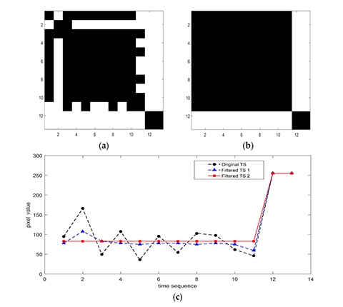
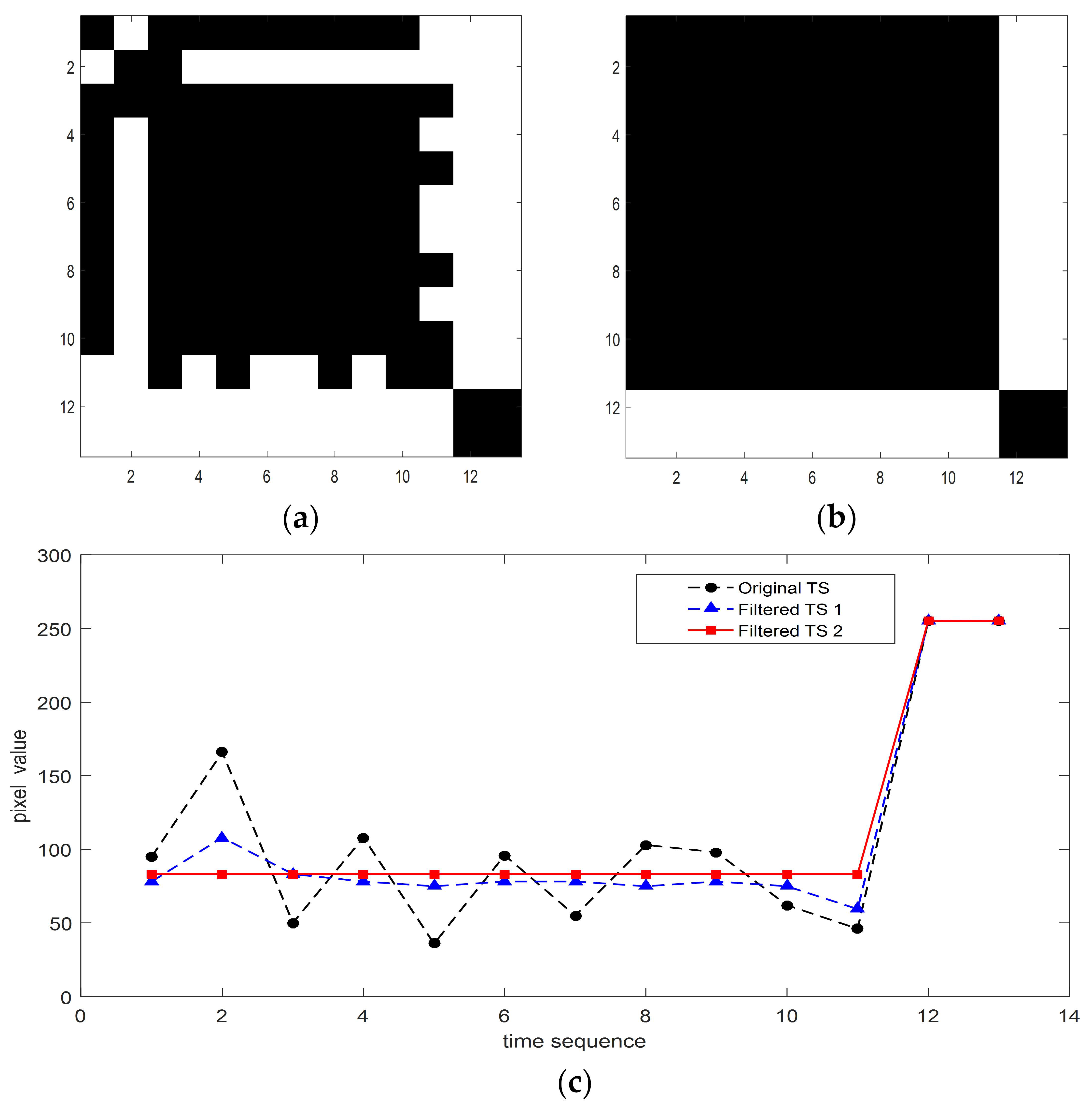
To illustrate the process of searching unchanged points, the analysis results of a pixel within the building areas are shown in Figure 13, where the buildings were constructed on the penultimate image in Dataset 1. Figure 13a is the similarity measure matrix obtained by the two-sample KS test from the first step, and Figure 13b shows the result of the second step using the STSLR test, which includes the similarity information of all pixels on the time-series in this position. It can be observed that the first matrix contains some erroneous results considered to be dissimilar, while in the second one, the wrong detection results are eliminated completely. Figure 13c shows the filtered results of all images based on the first and second similarity measure matrix, respectively, which indicates the advantages of the two-step strategy combining the proposed hypothesis testing method.

By suppressing the speckle noise, the multitemporal filtered SAR images can restore the structural features, including the contours, edges, and textures of real geographical information, considerably improve the image quality, and enable better interpretation of the image, especially for the high resolution SAR images, providing more reliable data for subsequent multitemporal applications such as forest monitoring, land cover change detection, and target recognition.

5. Conclusions

The traditional speckle suppression methods for SAR images either have the problem of resolution and detail information loss, or changes of the spatiotemporal information of the filtered images. To solve these problems, a novel multitemporal filtering method based on hypothesis testing was proposed, which can not only suppress the noise without the loss of spatial resolution, but also ensure the consistency of the images before and after filtering as far as possible. To combine the hypothesis testing approaches and improve the filtering results, the strategy of a two-step similarity measurement was conducted. In step 1, the similar patches for each date were extracted according to the bi-date analysis using the two-sample KS test method. Then, in step 2, a new test method called the STSLR test was proposed to process the patch stacks generated by the first step, which exploited the peculiarity of the multi-dimensional structure to further enhance the filtering results. By averaging the unchanged pixels, the final filtered images were obtained. To demonstrate the performance of the proposed method, we carried out the experiments using synthetic multitemporal SAR data and two real time-series datasets in Tongzhou District of Beijing, China, which contained different land cover types and were acquired from 2012 to 2016 by TerraSAR-X. Our method showed the best performance in terms of both the qualitative and quantitative results. However, there are still some deficiencies in this work that need to be improved. For example, the computational efficiency of the algorithm can be accelerated by parallel processing. Apart from that, more experiments with different scenes and resolutions can be performed to validate the effectiveness more adequately. In future research, we will consider combining the non-local method and our approach to further improve the filtering effect.

References

- Zhao, L.; Yang, J.; Li, P.; Zhang, L. Seasonal inundation monitoring and vegetation pattern mapping of the Erguna floodplain by means of a RADARSAT-2 fully polarimetric time series. Remote Sens. Environ. 2014, 152, 426–440. [Google Scholar] [CrossRef]
- Pal, S.; Majumdar, T.; Bhattacharya, A.K. ERS-2 SAR and IRS-1C LISS III data fusion: A PCA approach to improve remote sensing based geological interpretation. ISPRS J. Photogramm. Remote Sens. 2007, 61, 281–297. [Google Scholar] [CrossRef]
- Sun, W.; Shi, L.; Yang, J.; Li, P. Building Collapse Assessment in Urban Areas Using Texture Information From Postevent SAR Data. IEEE J. Sel. Top. Appl. Earth Obs. Remote Sens. 2016, 9, 3792–3808. [Google Scholar] [CrossRef]
- Gong, M.; Zhao, J.; Liu, J.; Miao, Q.; Jiao, L. Change detection in synthetic aperture radar images based on deep neural networks. IEEE Trans. Neural Netw. Learn. Syst. 2016, 27, 125–138. [Google Scholar] [CrossRef] [PubMed]
- Kleynhans, W.; Salmon, B.P.; Olivier, J.C. Detecting settlement expansion in South Africa using a hyper-temporal SAR change detection approach. Int. J. Appl. Earth Obs. Geoinf. 2015, 42, 142–149. [Google Scholar] [CrossRef]
- Schlaffer, S.; Matgen, P.; Hollaus, M.; Wagner, W. Flood detection from multi-temporal SAR data using harmonic analysis and change detection. Int. J. Appl. Earth Obs. Geoinf. 2015, 38, 15–24. [Google Scholar] [CrossRef]
- Arsenault, H.H. Speckle Suppression and Analysis for Synthetic Aperture Radar Images. Opt. Eng. 1986, 25, 636–643. [Google Scholar]
- Oliver, C. Information from SAR images. J. Phys. D Appl. Phys. 1991, 24, 1493. [Google Scholar] [CrossRef]
- Oliver, C.; Quegan, S. Understanding Synthetic Aperture Radar Images; Artech House: Boston, MA, USA; London, UK, 1998. [Google Scholar]
- Deledalle, C.A.; Tupin, F. Iterative Weighted Maximum Likelihood Denoising with Probabilistic Patch-Based Weights; IEEE Press: Piscataway, NJ, USA, 2009; pp. 2661–2672. [Google Scholar]
- Kuan, D.T.; Sawchuk, A.A.; Strand, T.C.; Chavel, P. Adaptive restoration of images with speckle. IEEE Trans. Acoust. Speech Signal Process. 1987, 35, 373–383. [Google Scholar] [CrossRef]
- Lee, J.S. Refined filtering of image noise using local statistics. Comput. Graph. Image Process. 1981, 15, 380–389. [Google Scholar] [CrossRef] [Green Version]
- Nicolas, J.M.; Tupin, F.; Maitre, H. Smoothing speckled SAR images by using maximum homogeneous region filters: An improved approach. In Proceedings of the IEEE 2001 International Geoscience and Remote Sensing Symposium (IGARSS 2001), Sydney, NSW, Australia, 9–13 July 2001; Volume 1503, pp. 1503–1505. [Google Scholar]
- Zhong, H.; Li, Y.; Jiao, L. SAR Image Despeckling Using Bayesian Nonlocal Means Filter with Sigma Preselection. IEEE Geosci. Remote Sens. Lett. 2011, 8, 809–813. [Google Scholar] [CrossRef]
- Lee, J.S. Digital Image Enhancement and Noise Filtering by Use of Local Statistics. IEEE Trans. Pattern Anal. Mach. Intell. 1980, PAMI-2, 165–168. [Google Scholar] [CrossRef]
- Kuan, D.T.; Sawchuk, A.A.; Strand, T.C.; Chavel, P. Adaptive Noise Smoothing Filter for Images with Signal-Dependent Noise. IEEE Trans. Pattern Anal. Mach. Intell. 2009, PAMI-7, 165–177. [Google Scholar] [CrossRef]
- Frost, V.S.; Stiles, J.A.; Shanmugan, K.S.; Holtzman, J.C. A model for radar images and its application to adaptive digital filtering of multiplicative noise. IEEE Trans. Pattern Anal. Mach. Intell. 1982, 4, 157–166. [Google Scholar] [CrossRef] [PubMed]
- Lee, J.-S.; Wen, J.-H.; Ainsworth, T.L.; Chen, K.-S.; Chen, A.J. Improved sigma filter for speckle filtering of SAR imagery. IEEE Trans. Geosci. Remote Sens. 2009, 47, 202–213. [Google Scholar]
- Lopes, A.; Touzi, R.; Nezry, E. Adaptive speckle filters and scene heterogeneity. IEEE Trans. Geosci. Remote Sens. 1990, 28, 992–1000. [Google Scholar] [CrossRef]
- Touzi, R. A review of speckle filtering in the context of estimation theory. IEEE Trans. Geosci. Remote Sens. 2003, 40, 2392–2404. [Google Scholar] [CrossRef]
- Ni, W.; Guo, B.; Yang, L. Speckle reduction algorithm for SAR images using contourlet transform. J. Inf. Comput. Sci. 2006, 3, 83–94. [Google Scholar]
- Hou, B.; Zhang, X.; Bu, X.; Feng, H. SAR Image Despeckling Based on Nonsubsampled Shearlet Transform. IEEE J. Sel. Top. Appl. Earth Obs. Remote Sens. 2012, 5, 809–823. [Google Scholar] [CrossRef]
- Argenti, F.; Alparone, L. Speckle removal from SAR images in the undecimated wavelet domain. IEEE Trans. Geosci. Remote Sens. 2002, 40, 2363–2374. [Google Scholar] [CrossRef]
- Xie, H.; Pierce, L.E.; Ulaby, F.T. SAR speckle reduction using wavelet denoising and Markov random field modeling. IEEE Trans. Geosci. Remote Sens. 2002, 40, 2196–2212. [Google Scholar] [CrossRef]
- Buades, A.; Coll, B.; Morel, J.M. A Review of Image Denoising Algorithms, with a New One. SIAM J. Multiscale Model. Simul. 2005, 4, 490–530. [Google Scholar] [CrossRef] [Green Version]
- Parrilli, S.; Poderico, M.; Angelino, C.V.; Verdoliva, L. A Nonlocal SAR Image Denoising Algorithm Based on LLMMSE Wavelet Shrinkage. IEEE Trans. Geosci. Remote Sens. 2012, 50, 606–616. [Google Scholar] [CrossRef]
- Trouve, E.; Chambenoit, Y.; Classeau, N.; Bolon, P. Statistical and operational performance assessment of multitemporal SAR image filtering. IEEE Trans. Geosci. Remote Sens. 2003, 41, 2519–2530. [Google Scholar] [CrossRef]
- Bruniquel, J.; Lopes, A. Multi-variate optimal speckle reduction in SAR imagery. Int. J. Remote Sens. 1997, 18, 603–627. [Google Scholar] [CrossRef]
- Coltuc, D.; Trouve, E.; Bujor, F.; Classeau, N. Time-space filtering of multitemporal SAR images. In Proceedings of the IEEE 2000 International Geoscience and Remote Sensing Symposium (IGARSS 2000), Honolulu, HI, USA, 24–28 July 2000; Volume 2907, pp. 2909–2911. [Google Scholar]
- Grandi, G.F.D.; Leysen, M.; Lee, J.S.; Schuler, D. Radar reflectivity estimation using multiple SAR scenes of the same target: Technique and applications. In Proceedings of the 1997 IEEE International Geoscience and Remote Sensing (IGARSS 1997), Remote Sensing—A Scientific Vision for Sustainable Development, Singapore, 3–8 August 1997; Volume 1042, pp. 1047–1050. [Google Scholar]
- Quegan, S.; Toan, T.L.; Yu, J.J.; Ribbes, F.; Floury, N. Multitemporal ERS SAR analysis applied to forest mapping. IEEE Trans. Geosci. Remote Sens. 2000, 38, 741–753. [Google Scholar] [CrossRef]
- Lê, T.T.; Atto, A.M.; Trouvé, E.; Nicolas, J.M. Adaptive Multitemporal SAR Image Filtering Based on the Change Detection Matrix. IEEE Geosci. Remote Sens. Lett. 2014, 11, 1826–1830. [Google Scholar] [Green Version]
- Su, X.; Deledalle, C.A.; Tupin, F.; Sun, H. Two-Step Multitemporal Nonlocal Means for Synthetic Aperture Radar Images. IEEE Trans. Geosci. Remote Sens. 2014, 52, 6181–6196. [Google Scholar]
- Chierchia, G.; Gheche, M.E.; Scarpa, G.; Verdoliva, L. Multitemporal SAR Image Despeckling Based on Block-Matching and Collaborative Filtering. IEEE Trans. Geosci. Remote Sens. 2017, 55, 5467–5480. [Google Scholar] [CrossRef]
- Freeman, A. SAR calibration: An overview. IEEE Trans. Geosci. Remote Sens. 1992, 30, 1107–1121. [Google Scholar] [CrossRef]
- Townshend, J.R.; Justice, C.O.; Gurney, C.; McManus, J. The impact of misregistration on change detection. IEEE Trans. Geosci. Remote Sens. 1992, 30, 1054–1060. [Google Scholar] [CrossRef] [Green Version]
- Wegmüller, U.; Werner, C.L. Gamma SAR processor and interferometry software. Eur. Space Agency Spec. Publ. 1997, ESA SP-414, 1686–1692. [Google Scholar]
- Lv, X.; Yazıcı, B.; Zeghal, M.; Bennett, V.; Abdoun, T. Joint-Scatterer Processing for Time-Series InSAR. IEEE Trans. Geosci. Remote Sens. 2014, 52, 7205–7221. [Google Scholar]
- Deledalle, C.-A.; Denis, L.; Tupin, F. How to compare noisy patches? Patch similarity beyond Gaussian noise. Int. J. Comput. Vis. 2012, 99, 86–102. [Google Scholar] [CrossRef] [Green Version]
- Baglivo, J.A. Mathematica Laboratories for Mathematical Statistics: Emphasizing Simulation and Computer Intensive Methods; SIAM: Philadelphia, PA, USA, 2005; Volume 14. [Google Scholar]
- Cozzolino, D.; Parrilli, S.; Scarpa, G.; Poggi, G.; Verdoliva, L. Fast Adaptive Nonlocal SAR Despeckling. IEEE Geosci. Remote Sens. Lett. 2013, 11, 524–528. [Google Scholar]
- Xie, H.; Pierce, L.E.; Ulaby, F.T. Statistical properties of logarithmically transformed speckle. IEEE Trans. Geosci. Remote Sens. 2002, 40, 721–727. [Google Scholar] [CrossRef]
- Martino, G.D.; Poderico, M.; Poggi, G.; Riccio, D.; Verdoliva, L. Benchmarking Framework for SAR Despeckling. IEEE Trans. Geosci. Remote Sens. 2013, 52, 1596–1615. [Google Scholar] [CrossRef]
Figure 1.
The processing flow of the proposed filtering method.
Figure 2.
Two cases in multi-date analysis using the sliding time-series likelihood ratio (STSLR) test.
Figure 3.
Filtering results of the image “Hill” corrupted by simulated speckle (first scene with unchanging and 1-Look noise): (a) Reference image (noise-free); (b) Noisy with single-look; (c) Fast adaptive nonlocal SAR despeckling (FANS); (d) Change detection matrix based filter (CDMF); (e) Quegan’s filter (QF); (f) Multitemporal SAR block-matching and 3D filtering (MSAR_BM3D); (g) Proposed.
Figure 4.
Filtering results of the image “Hill” corrupted by simulated speckle (first scene with changing and 1-Look noise): (a) Reference image (noise-free); (b) Noisy with single-look; (c) FANS; (d) CDMF; (e) QF; (f) MSAR_BM3D; (g) Proposed.
Figure 5.
Filtering results of the image “Hill” corrupted by simulated speckle (first scene with unchanging and 4-Looks noise): (a) Reference image (noise-free); (b) Noisy with single-look; (c) FANS; (d) CDMF; (e) QF; (f) MSAR_BM3D; (g) Proposed.
Figure 6.
Filtering results of the image “Hill” corrupted by simulated speckle (first scene with changing and 4-Looks noise): (a) Reference image (noise-free); (b) Noisy with single-look; (c) FANS; (d) CDMF; (e) QF; (f) MSAR_BM3D; (g) Proposed.
Figure 7.
Two time-series datasets of TerraSAR-X remote sensing images in Tongzhou District of Beijing: (a) Dataset 1 (first scene); (b) Optical image; (c) Dataset 2 (1st scene); (d) Optical image.
Figure 8.
Filtering results for Dataset 1: (a) Original image (22 January 2012); (b) FANS; (c) QF; (d) CDMF; (e) MSAR_BM3D; (f) the proposed approach.
Figure 9.
Preservation of strong target points for Dataset 1. (a) Original image (22 January 2012); (b) FANS; (c) QF; (d) CDMF; (e) MSAR_BM3D; (f) the proposed approach.
Figure 10.
Change trends of the indices for Dataset 1: (a) ENL; (b) Mean bias (negative logarithm).
Figure 11.
Filtering results for Dataset 2: (a) Original image (28 March 2012); (b) FANS; (c) QF; (d) CDMF; (e) MSAR_BM3D; (f) the proposed approach.
Figure 12.
Preservation of strong target points for Dataset 2. (a) Original image (28 March 2012); (b) FANS; (c) QF; (d) CDMF; (e) MSAR_BM3D; (f) the proposed approach.
Figure 13.
The similarity measurement matrix from the two-step strategy of Dataset 1: (a) Step 1; (b) Step 2; (c) filtering results of a pixel within the changeable building areas.