1. Introduction
Karstification is a long-term dissolution process of water acting over carbonate rocks such as limestone, dolomite and other soluble rocks; dissolution is continuous, making karstification an unceasing and evolving process. Thus, Karst refers to a three-dimensional open system in which dissolution has already modified the surface and subsurface, thereby displaying characteristic features such as dolines, caves and conduit networks. Dolines (sinkholes) are usually bowl-shape, enclosed depressions at surface level, evolved as a consequence of the dissolution of carbonate rocks. Dolines can act as connectors between surface water and groundwater, collecting and draining rainfall into the subsurface [
1].
Doline internal drainage and morphometric characteristics can serve to diagnose karst development and other endokarst features [
2,
3]. Although the term “doline” is widely known, its definition varies significantly across literature and current depressions classifications [
4]. Ford and Williams [
2] presented a doline classification of six main types according to their forming process, whilst morphometric attributes are additional characteristics to further subdefine dolines [
5].
Doline mapping plays a key role in the development of management strategies with a focus on subsidence risk, land use planning and groundwater vulnerability [
6,
7,
8]. Regarding the latter, dolines in karst terrains exert great influence on vulnerability outcomes due to their hydrological behavior, which allows a faster transport of pollutants from surface to water table. Doline patterns and alignments also aid with inferences regarding subsurface karst development, such as epikarst and conduit systems, due to their association with joints and faults [
9,
10]. Despite the importance of doline mapping, their allocation either by fieldwork or imagery analysis is time consuming for large karst areas. On the other hand, doline estimation from topographic maps is highly dependent on several factors including map scale, doline size and contour interval [
11].
Remote sensing and geographic information systems (GIS) are nowadays important tools to analyze and study karst areas and landforms [
12,
13,
14]. With the increase of available remote-sensing data, several GIS-based processes for surface depression estimation have been proposed [
15,
16]. Automatic or semiautomatic depression mapping methods, based on digital elevation models (DEMs), represent a great advantage against visual or manual delineation when study areas are considerable in size or where vegetation is dense. Nevertheless, automated extraction of specific types of landforms from DEMs still remains as a challenge [
17]. High-resolution data does not always reflects better results, as in the case of depression analysis. The number of depressions tends to increase when high-resolution DEMs are applied, making necessary an extra analysis to eliminate artificial depressions. On the other hand, coarser DEMs also affect depressions estimation since depressions smaller than the grid size can be not defined. Therefore, effects of cell resolution or DEM accuracy on results must be always considered [
18].
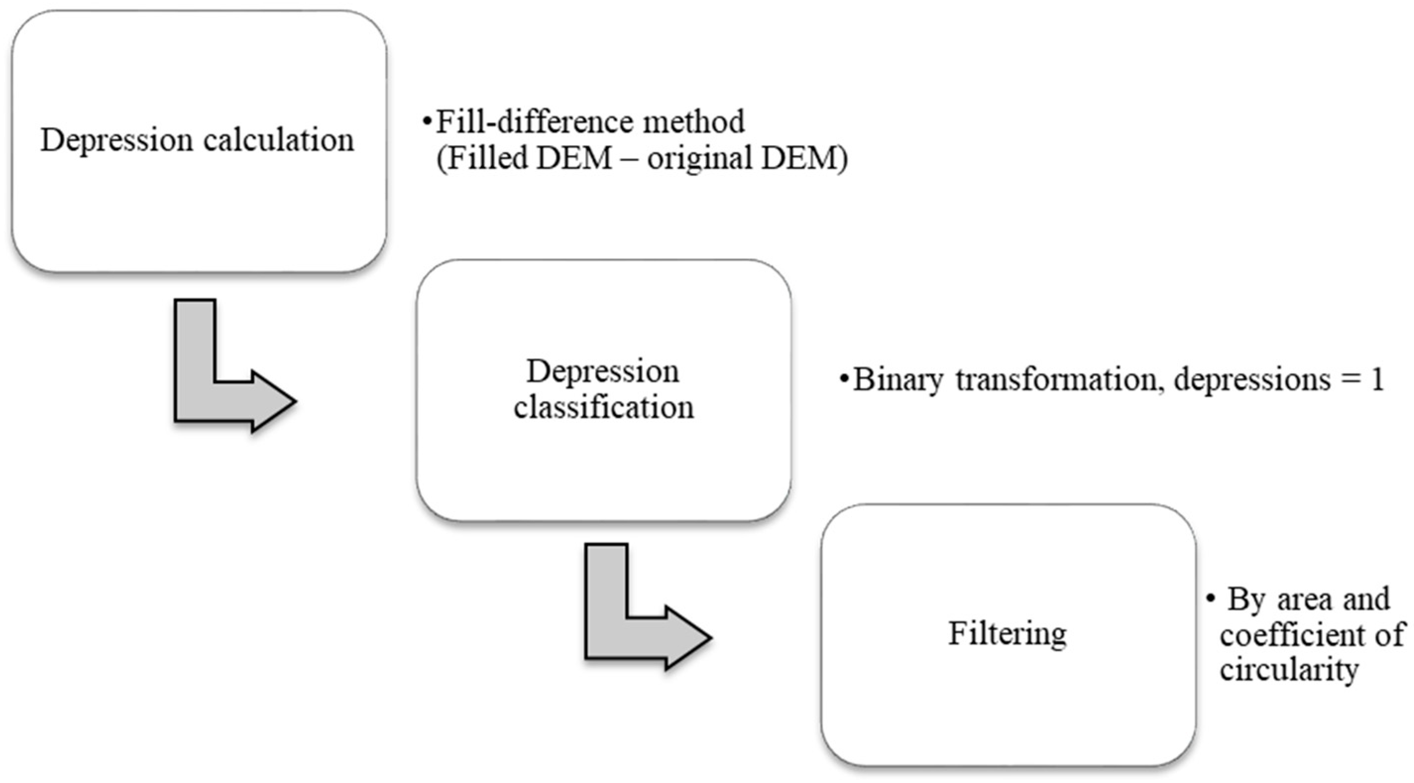
Diverse schemas for doline estimation have been introduced and tested in multiple karst areas [
19,
20]; as shown in
Figure 1, the fill-difference method is the arithmetic procedure most utilized as a base for doline mapping [
9,
21,
22]. This fill-difference is based on the Fill tool, part of the ArcHydro toolset of ArcGIS. The Fill algorithm elevates the value of DEM pixels representing depressions or sinks (including those that are spurious) to create a hydrological “corrected” continuous surface [
23]. To estimate depressions areas and depths, a subtraction between the original DEM and the filled DEM is performed. The obtained DEM, representing depressions, is then converted into a binary raster (1 = depression) to highlight depressions before performing a morphometric analysis to further classify depressions as dolines or any other depression of interest.
The majority of literature apply a defined depth as a threshold, which is subjective and study area-dependent. This threshold serves to decrease the number of spurious dolines from the surface. Nevertheless, this approach may not define dolines being contained in larger depressions or located at depths under the assigned threshold value, even if this threshold has demonstrated the best overall accuracy for a given area. To solve this problem, a new methodology is presented in this work with the goal of allocating dolines at variable depths and improve doline mapping using DEMs in large karst areas.
The new proposed method for dolines mapping is evaluated on a study area located in the Yucatan Peninsula, an interesting karst area with unique features like “Cenotes” (open dolines exposing water) and a semicircular doline alignment. This is a side-study derived from the IKAV project, part of the INOWAS group, which aims to develop an integrated karst aquifer vulnerability approach. Initially, four European groundwater vulnerability methodologies where applied in the Yucatan state (hereinafter Yucatan) to determine the congruence between vulnerability outcomes and regional features. The results showed a strong influence of some parameters on specific vulnerability categories; dolines were presented as a key feature, resulting in high vulnerability rates according to different methodologies [
25]. Nevertheless, the current doline map of the region is based on contours, at 10-m intervals, classified as depressions [
26,
27,
28]; Yucatan being a nearly flat area, a considerable number of dolines were not mapped due to such large intervals, affecting outcomes from groundwater vulnerability maps. Therefore, an accurate doline mapping in Yucatan is imperative in order to define areas of high doline density more efficiently due to its influence in groundwater vulnerability mapping.
A semiautomatic multidepth threshold approach (hereinafter MDTA) is proposed, taking advantage of the multiple tools available in GIS software. Additionally, a filter based on “depressions-containing depressions” (DCD), or nested dolines, is tested and included to decrease the number of spurious dolines and to improve accuracy. After testing different scenarios and parameters, the MDTA demonstrates higher accuracy, precision and sensitivity values in comparison with single-depth thresholds.
2. Materials and Methods
2.1. Study Area
Yucatan (39,524 km
2) is located in the south of Mexico and is the northernmost part of the Yucatan peninsula, which includes two other Mexican states (Campeche and Quintana Roo) and the northern part of the Central American countries of Belize and Guatemala. The peninsula is formed by an emerged limestone platform of about 165,000 km
2, in which groundwater flow is primarily dominated by turbulent conduit flow due to a well-developed conduit system at variable scale ranges [
29]. According to Weidie [
30], the dominant sediments in the Peninsula are limestone and dolomite from the Eocene or younger epochs reaching thicknesses > 1500 m. Lugo-Hubp [
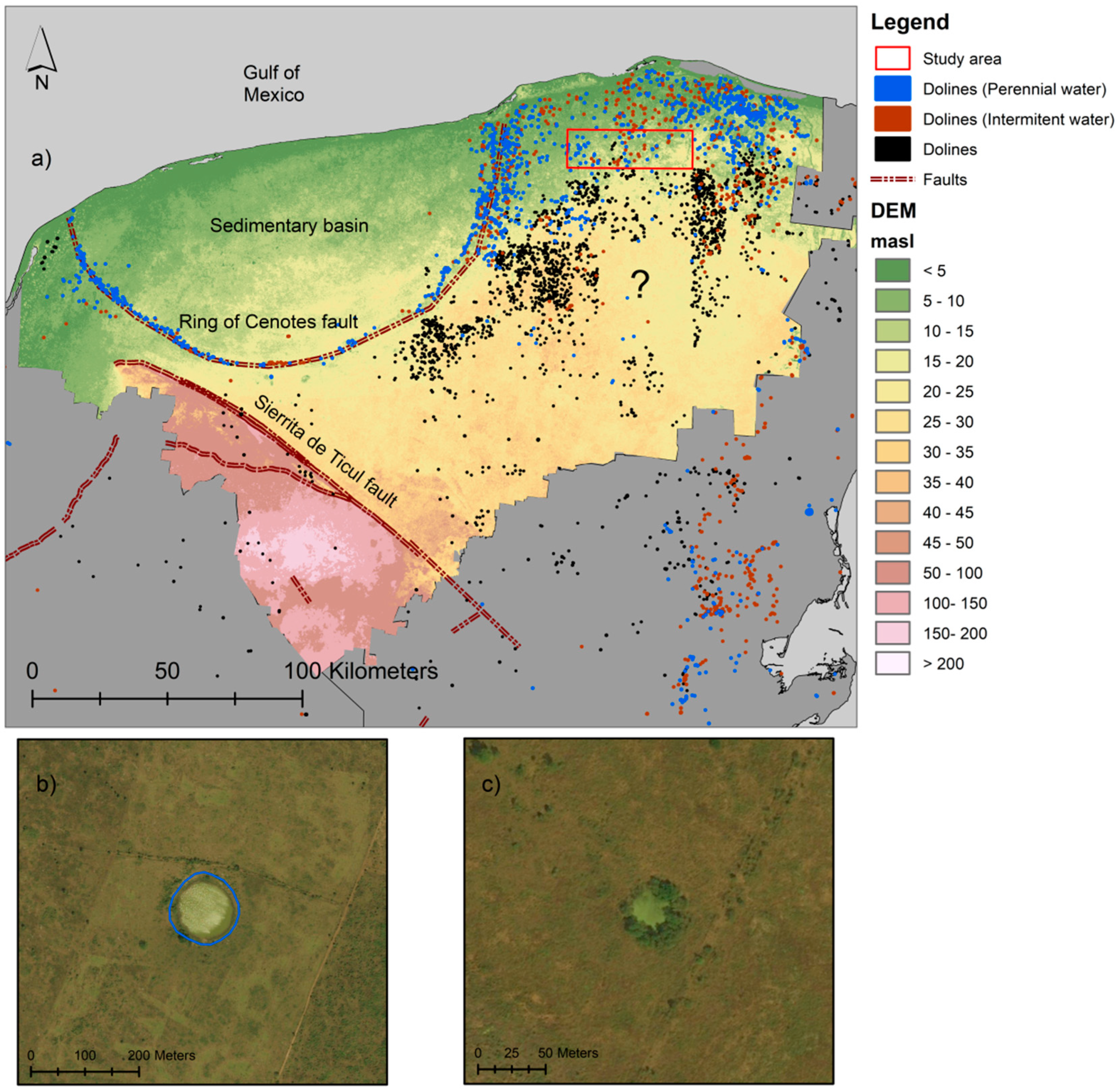
26] divided the Yucatan peninsula into two main morphological units according to morphology and stages of karst formation: A relatively young area in the north where Neogene sedimentary rocks predominate with high number of dolines and an older area in the south with Paleogene sedimentary rocks exposing little doline development (
Figure 2). Two important doline areas have been highlighted in Yucatan; the Ring of Cenotes and the North-eastern Yucatan [
27,
28,
31]. At the north of the peninsula a sedimentary basin was formed after the impact of an asteroid at the end of the cretaceous [
27].This sedimentary basin is hydrogeologically delimited by the Ring of Cenotes. The Ring of Cenotes is a fringe of high doline density displaying a semicircular alignment of about 180 km diameter [
32]. The ring, acting as a groundwater divide due to high conductivity, intercepts water flowing from South, discharging to the sea. This divergence in flow can be the cause for the low development of karst features inside the sedimentary basin and the considerable number of dolines delineating the crater rim. Doline distribution in other areas have shown a strong relationship with tectonic structure rather than lithology based on correlations of karst depressions distribution with gravity anomalies and topography [
28]. The Ring of Cenotes is a regional fault which development is associated to differential lithological compaction within the sedimentary basin, a buried reef complex or impact breccia collapse [
33]. The ring is also a boundary between fractured limestone and the unfractured limestone inside the ring [
27]. A broader lithology description from the analysis of drilling cores, can be found in the work of Rebolledo Vieyra [
34]. With the exception of the Ring of Cenotes, evolution of karst landforms in Yucatan is associated with tectonics and the fluctuation of sea level during the quaternary and previous epochs [
26]. In the case of the Northeast doline field, the influence of dynamic interactions between the limestone near the coast and seawater seems to have triggered the high development of dolines due to limestone dissolution [
35]. Another important regional feature is the Sierrita de Ticul fault line [
29]. This fault acts as a flow barrier with hydraulic heads declining toward the northeast [
36]; this could explain the lack of dolines in the plain located at North of this fault line.
In Yucatan, topography presents elevations above sea level varying from centimeters along the coast to approximately 30 m inland with the exception of a hill area located at the southern part of Yucatan where elevation is up to 205 m [
39]. The flat topography of the region and considerable karstification allow infiltration to act at fast rates without runoff generation [
40]; this makes groundwater the only source for water supply in Yucatan [
41].
Data from the National Meteorological Service shows a mean annual precipitation of about 1100 mm/year in a seasonal pattern, with intensities varying from 10 to 20 mm/day [
42]. Precipitation also varies spatially; the coastal area in the northwest receives an average of 550 mm/year and is thus relatively dry, whilst the Yucatan south eastern region receives up to 1500 mm/year. Yucatan water balance is positive with an estimated recharge varying from 14% to 20% of the mean annual precipitation [
38,
39,
40].
Soils are generally absent or shallow with a thickness less than 7 cm for Lithosols and Luvisols [
43,
44]. Rendzinas predominate covering approximately 46% of the Yucatan area according to public maps [
45]. Soil texture is variable, with coarse and fine soils distributed along Yucatan but showing dominance of medium textures in central areas. Vegetation maps show deciduous forest to prevail, with mangroves and sand dunes along the coastal area [
45].
Dolines are a common feature in Yucatan and many of them intersect the shallow water table exposing water. Doline density is variable from areas with several dolines per square kilometers to several kilometers between them [
46]. Diameters of dolines located in the Ring of Cenotes vary from 50 to 500 m with depths ranging from 2 to 120 m [
47,
48]. These values show agreement with averages of 4900 mapped dolines displaying a mean diameter of 104 m with a mean area of 8600 m
2. However, smaller dolines, clearly visible from imagery, are dispersed in Yucatan. Contour maps at 1:50,000 scale, publicly available from the National Institute of Geography and Statistics (INEGI), are the base for the latest doline map of the region (
Figure 3a). From contours maps, Aguilar [
49] performed a morphometric analysis on contours defined as depressions and water bodies (perennial and intermittent) to categorize dolines (
Figure 3b). However, the contour maps at 10 m intervals tend to overlook shallow or small dolines. Also, inaccuracies in contours classification can derive in areas without dolines, thus affecting further analysis. Therefore, methodologies to dolines mapping based on DEMs can aid on doline mapping without extensive fieldwork. As the area is mostly a flat plain with elevations gradually increasing southward, the use of the fill-difference method with a single threshold to estimate dolines is potentially inappropriate since dolines contained by larger depression areas will not be mapped. To address this problem the MDTA is proposed. This method was tested in a 652 km
2 study area located in North-eastern Yucatan and evaluated against 545 dolines mapped by visual inspection of high-resolution imagery (0.3 m resolution). It is important to note that the study area contains just 144 dolines according the 1:50,000 contour maps, where 117 coincide with those mapped from imagery analysis. Inconsistencies are associated with doline size since those dolines holding an area smaller than 50 m in diameter are not mapped (
Figure 3c).
2.2. Material and Methods
The suggested method for doline mapping in nearly flat karst terrains is a semiautomatic approach based solely on GIS software. In this work, ArcGIS version 10.5 is used and the ArcBruTile extension served to display Google Earth imagery at high resolution directly in ArcGIS. A digital-elevation model with 5 × 5-m grids, derived from light detection and ranging data (LiDAR) with 1 m of vertical resolution, was obtained from public databases for this study [
50]. The DEM in raster format was corrected for no data values prior to being run in our analysis. Data correction was performed by filling null data with averages of the surrounding grids by the moving window method. In this paper, doline refers to any enclosed depression falling into defined morphometric attributes without consideration of their development characteristics.
The proposed MDTA is based on the fill-difference method to highlight depression areas but, unlike previous works, we suggest the use of multiple depth intervals, statistically classified, to improve dolines mapping. In other words, this method defines dolines at different depths to subsequently merge those which overlap to avoid mapping the same doline at variable depths. The MDTA consists of four steps: Depressions estimation, depressions classification, vectorization and filtering. The use of the model builder function of ArcGIS simplifies the implementation of the method if some parameters in the calculation, for example the number of intervals, minimum polygon area and minimum Gravelius coefficient, are previously defined.
As displayed in
Figure 4, in step one, a DEM without “No data” values is modified into a depression-free DEM applying the Fill algorithm (1). Subtraction of the original DEM from the filled DEM by Raster calculator (2) results in a new raster displaying depressions. Transformation of the depression raster into binary data to differentiate depressions from no-depression grids is no longer necessary due to the application of an optimization method in the next step.
Step two aims to classify depressions into multiple intervals utilizing the Slice algorithm (3). The Jenks optimization method [
51] was chosen in order to reduce the variance between values contained in a given depression interval and to increase the variance between different intervals; this classification serves to highlight depressions contained in larger depressions including those that are shallow. The number of optimized depth classes by Jenks can be adjusted according the depressions map range; in this work, a 10-class optimization was defined. To prepare our depression raster to be converted into a refined polygon shape file, Contour (4) and Smooth line (5) tools were run.
Creation of polygons, deleting contours representing hills and the calculation of morphometric parameters are part of step three. Polygons are vectorized from contours executing the Feature to polygon (6) algorithm; therefore, polygons will represent depressions shape at ten different depths (Jenks classes). A closed contour typifies a peak if it holds the same value as the contour containing it. The Dissolve (7) tool eliminates peaks inside a closed depression and must be applied to each Jenks class separately. The next task is to calculate a compactness coefficient for each polygon in a new field created by the Add a new field (8) tool. The Gravelius coefficient estimates the ratio between the perimeter of a given watershed (or doline) and the circumference of a circle with the same area as the studied watershed [
52]; this is expressed by the equation:
where
Gc denotes the Gravelius coefficient,
P is the perimeter and
A is the area of the studied two-dimensional landform. In so far as
Gc approaches 1, the watershed holds a more circular shape. The circularity index has been widely used as morphometric estimator for watersheds and dolines [
53,
54]. To settle a maximum Gravelius value, a statistical morphometric analysis was run for the 545 dolines mapped by imagery. In this work, depressions with
Gc ≤ 1.04 are categorized as dolines.
Step four focuses on the filtering of polygons by morphometric attributes and location to define dolines. Using the Select by Attributes (9) tool, polygons with values of Gc > 1.04 are eliminated with the Delete Features (10) tool. A minimum area of 900 m2 was chosen to classify depressions as dolines, to be able to compare our results with outcomes of the MDTA using a DEM of 30×30-m resolution (manuscript in preparation). Finally, a location filter was applied to decrease uncertainty. Using the Select by location (11) data management tool, dolines containing dolines were selected and saved in a final shapefile. This filter was included in the MDTA after testing two scenarios with different settings for the Jenks classification. To avoid overestimations due to the possibility of mapping the same doline at different depths, the Merge (12) and Dissolve (13) tools are applied once more.
In this work, three scenarios were applied. Scenario 1 analyzes depressions classified statistically by Jenks intervals with base 0; scenario 2 eliminates depressions of less than 2 m, or Jenks base 2, aiming to eliminate spurious dolines; finally, scenario 3 implements the DCD filter aiming to reassert true dolines.
2.3. Sensitivity and Accuracy
A binary analysis to test accuracy overlapped estimated dolines over 545 dolines mapped by high-resolution imagery. Sensitivity (true positives rate), precision (positive prediction value) and accuracy were calculated for single-depth thresholds and the MDTA in three scenarios according to:
where
TP is the number of estimated dolines matching those from imagery analysis (true positives);
FP are those estimated without match (false positives) and
FN are dolines from imagery which are not overlapped by estimated ones (false negatives).
It is important to mention that unknown dolines, mainly in vegetation covered areas, which we were unable to map by visual interpretation, are likely to exist. This directly affects the accuracy analysis since estimated dolines not matching those from imagery were automatically considered false positives.
3. Results and Discussion
Application of the Slice algorithm classifying Jenks at base 0, or scenario 1, arose in a considerable number of estimated dolines, mostly for intervals near the surface. The effects of this overestimation were clearer for the MDTA with more than 4000 probable dolines with around 3500 categorized as FP. A random selection of 200 dolines from the MDTA served as a subsample to check their match with imagery; more than 180 dolines were not visible even in areas with sparse vegetation. In general, MDTA for scenario 1 performed poorly with an accuracy of 12% due to the high number of FP. To minimize this probable overestimation, the model was run again setting a base of 2 m for the Jenks classification, or scenario 2. Jenks base for this scenario was defined after the analysis of depressions depth on the area. This procedure aimed to decrease the number of shallow dolines near the surface and improve accuracy.
The MDTA performed better as estimated dolines and FP decreased by 43% and 68%, respectively, from their initial numbers. Setting against single thresholds and MDTA for both scenarios, the latter displayed the highest TP rate with a constant value of 472 matching dolines in both cases. This indicates that a Jenks classification starting at 2-m depth eliminates a considerable amount of shallow dolines without influencing TP. Therefore, accuracy was improved from 12% to 39% with sensitivity remaining at 80% as shown in
Figure 5. Despite this upgrade, the MDTA accuracy was still lower than those displayed by some single thresholds. In this case, employment of a single threshold seemed to be more plausible since the highest accuracy was found for a depth of 3.5 m with 48%.
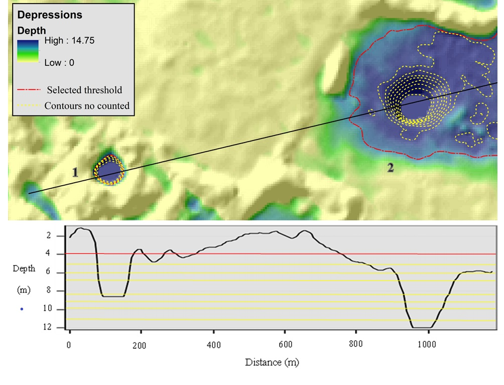
With estimated dolines still outnumbering those from imagery by more than 50% in scenario 2 and the overlook of dolines under the assigned depth threshold (
Figure 6), an extra process to filter spurious dolines was necessary. When analyzing single threshold patterns, it was noticed that estimated, TP and FP show a positive trend with regard to depth; the deeper the doline, the more likely to be mapped and to be true. According to this statement, a filter of depressions-containing depressions (DCD) was applied as scenario 3.
Incorporation of the DCD filter improved the MDTA performance for a final accuracy of 63% (
Table 1). True positives remained almost constant in all scenarios. This supports the idea of the DCD as a filter to decrease the number of spurious dolines, hence the number of FP, without affecting TP. Despite a minimum decline in sensitivity, precision and accuracy show improvements of 29% and 24%, respectively. Unlike scenarios 1 and 2, no single threshold displays a better accuracy than MDTA. In
Table 1, a 2.9-m depth displays the best accuracy with 47%. Nevertheless, this value is mostly triggered by a low number of estimated dolines compared with those from imagery, rather than as the result of a good match.
Our results indicate efficiency of the MDTA for doline mapping, especially when Jenks with a base >0 and the DCD filter are applied. However, more investigations regarding Jenks starting base for depth and number of classification are suggested to verify their influence on other karst areas. The DCD seems to be a precise step to reassert true dolines and decrease uncertainty of false positives.
Table 2 summarizes results obtained from three MDTA scenarios highlighting the influence of estimated dolines on final accuracy and how application of the DCD filter improved it. The impossibility of allocating dolines in dense vegetation areas by high-resolution imagery creates uncertainty of FP that could be in reality TP.
It is also important to consider the repercussions of high-resolution data in the analysis; the massive number of estimated depressions, mostly at shallow depths, directly affects accuracy. This is a consequence of the superior level of detail of DEM derived from LiDAR, therefore, application of the MDTA with coarser resolution DEMs is recommended as further analysis. DEM-derived attributes like slope or topographic position index (TPI) serving either as additional features or as base to map out dolines, could present some problems when high-resolution DEMs are used. Small details at surface-level are more evident, obstructing dolines identification. An advantage of this method is that no other DEM-derived data is necessary for the analysis.
In Yucatan, some dolines hold water during the rainy season; water residence time in dolines, characterized as intermittent water bodies, is expected to be short due to karstification and the high evapotranspiration rates. Those identified as perennial intersect the water table of which variation is in the range of centimeters due to the characteristics mentioned before. However, precipitation must be considered as an influencing factor for dolines mapping since water table fluctuations during wet-dry seasons can change the depth and shape of depressions. Acquisition date of the data is fundamental if the method is applied in areas with high water table variations.
Our results indicate an underestimation of dolines derived from contour maps. Therefore, digitalized maps from INEGI cannot be taken as an accurate source to display karst features to be used in further studies where doline density is a key feature. The scale of the original map and the near flat topography affects the location of dolines with depths of less than 10 m and areas smaller than 50 m of diameter. Also, dolines can be excluded due to human errors during the digitalizing process as we can see on
Figure 3. Comparing the 665 dolines mapped by the MDTA against the 144 from contour maps in an area of 652 km
2 reflects a difference in doline density of 0.79 dolines/km
2. This difference is considerable when doline density is imperative as in the case of groundwater vulnerability analysis. Use of DEMs to estimate dolines seems more plausible. However, depressions depth must be discretized in intervals, statistically classified, to define dolines to increase the accuracy.
4. Conclusions
In this work, we propose a new approach based solely on GIS tools for doline mapping utilizing a DEM derived from LiDAR with 5-m resolution. The MDTA is composed of four steps including the fill-difference method to estimate depressions. Application of statistics to segregate depressions into multiple classes enhances differences between depth intervals, thereby expediting the allocation of dolines contained in larger depressions. In addition to morphological filters like area or circularity index, a “depressions-containing depressions” filter (DCD) was also tested and included as an essential part of the method.
A total of 665 dolines were mapped and compared against 545 located by high-resolution imagery with 464 matching spatially. The MDTA demonstrates an accuracy of 63% for doline mapping. This moderate value is strongly driven by FP due to the impossibility of allocating all existing dolines by high-resolution imagery in dense vegetation areas; therefore, a considerable amount of FP could be in reality TP, which would display an increment in accuracy. If we contemplate the satisfying MDTA performance according to its sensitivity of 85%, the methodology is able to map out dolines substantially better than those utilizing a single threshold. Sensitivity, precision and accuracy show equilibrated percentages, highlighting the MDTA method as an excellent option for doline mapping in karst landscapes. Furthermore, this work demonstrates the current underestimation of dolines in Yucatan by previous works after comparing the results with dolines derived from 1:50,000 contour maps in a 652 km2 study area. However, LiDAR data covering Yucatan is sparse encouraging testing of the MDTA method with lower- and higher- resolution DEMs.


