Speckle Noise Reduction Technique for SAR Images Using Statistical Characteristics of Speckle Noise and Discrete Wavelet Transform


Department of Electronics and Computer Engineering, Hanyang University, 222, Wangsimni-ro, Seongdong-gu, Seoul 04763, Korea
*
Author to whom correspondence should be addressed.
Remote Sens. 2019, 11(10), 1184; https://0-doi-org.brum.beds.ac.uk/10.3390/rs11101184
Submission received: 2 May 2019
/
Revised: 14 May 2019
/
Accepted: 14 May 2019
/
Published: 18 May 2019
(This article belongs to the Special Issue Image Optimization in Remote Sensing)
Abstract
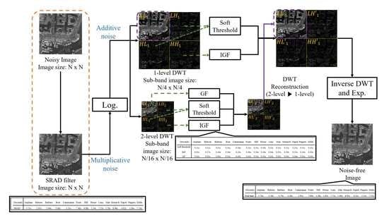
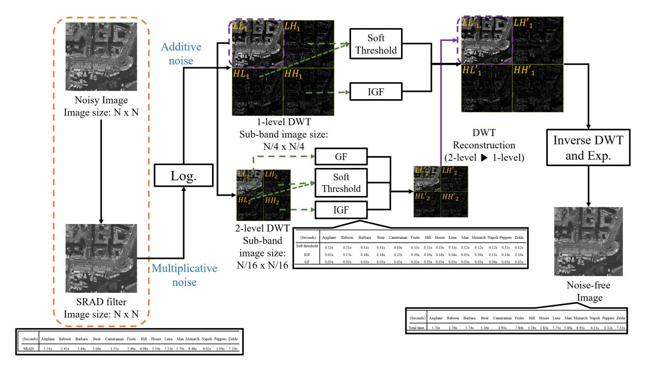
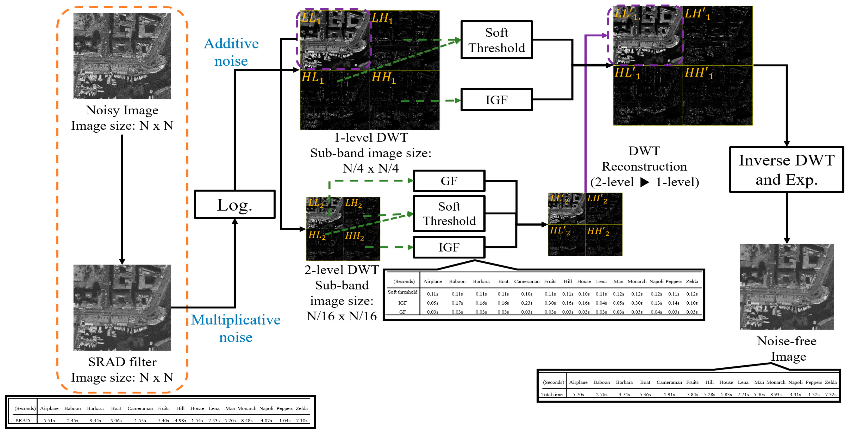
:Synthetic aperture radar (SAR) images map Earth’s surface at high resolution, regardless of the weather conditions or sunshine phenomena. Therefore, SAR images have applications in various fields. Speckle noise, which has the characteristic of multiplicative noise, degrades the image quality of SAR images, which causes information loss. This study proposes a speckle noise reduction algorithm while using the speckle reducing anisotropic diffusion (SRAD) filter, discrete wavelet transform (DWT), soft threshold, improved guided filter (IGF), and guided filter (GF), with the aim of removing speckle noise. First, the SRAD filter is applied to the SAR images, and a logarithmic transform is used to convert multiplicative noise in the resulting SRAD image into additive noise. A two-level DWT is used to divide the resulting SRAD image into one low-frequency and six high-frequency sub-band images. To remove the additive noise and preserve edge information, horizontal and vertical sub-band images employ the soft threshold; the diagonal sub-band images employ the IGF; while, the low- frequency sub-band image removes additive noise using the GF. The experiments used both standard and real SAR images. The experimental results reveal that the proposed method, in comparison to state-of-the art methods, obtains excellent speckle noise removal, while preserving the edges and maintaining low computational complexity.
1. Introduction
Synthetic Aperture Radar (SAR) images employ active sensors that detect microwave radiation, which has longer wavelength than visible light that is detected in passive sensors, such as the optical sensor. Therefore, the surface of the Earth can be observed at high resolution, regardless of weather conditions and sun phenomena [1]. The active sensor of SAR images is also used with satellites or unmanned aerial vehicles (UAVs), as the development of the active sensor technology applied to SAR images enabled high-resolution target detection and identification. SAR images are widely used in applications of a variety of fields, such as the military, agricultural, weather forecasting, and environmental analysis, etc. [2]. Due to the advantages of SAR images and their various applications, research on the technology behind SAR images is being actively conducted around the world (image enhancement [3,4,5], image classification [6,7], image segmentation [8,9], etc.).
In contrast with the optical sensor, the active sensor of the SAR is accompanied by speckle noise that arises from the coherent imaging mechanism. Speckle noise in SAR images is generated by the random interference of many elementary reflectors within one resolution cell [10]. This noise has different features from the noise observed in images that were obtained by passive sensors, such as the optical sensor. Speckle noise appears as a form of multiplicative noise in SAR images and it has the characteristics of a Rayleigh distribution [11]. SAR images are used by observers to extract information and identify targets. Speckle noise degrades SAR images and thus interferes with the transfer of image information to the observer. Therefore, the development of effective filtering methods in the reduction of speckle noise is critical for the analysis of information that is contained in various SAR images.
Numerous studies have been conducted with the aim of extracting image information from SAR images by removing speckle noise. Five main categories of methods were applied in these studies: linear filtering, nonlinear filtering, partial differential equation (PDE) filtering, hybrid methods, and filtering methods that are based on the discrete wavelet transform (DWT).
The linear filter convolutes an image with a symmetric mask and then reconstructs each pixel value as a weighted average value of the neighboring pixel values. The mean filter and the Gaussian filter are typical linear filtering techniques that are effective in simple and smoothing speckle noise reduction. A mean value of several pixel values around the target pixel substitute the mean filter. The target pixel is located in the center. The mean filter exhibits a low-edge preservation performance, because it does not consider the flat and homogeneous areas in the image [12]. The Gaussian filter uses a Gaussian function of two dimensions (2D) as a convolution mask. This filtering technique uses the Gaussian function as the mask weight value. The Gaussian function gives a larger weight to the center of the mask. Moreover, the Gaussian filtering technique shows excellent performance in terms of noise removal with a small variance; however, a blurring phenomenon appears in the edge areas.
The nonlinear filter extracts the edge regions in the image while using the statistical values (e.g., mean, median, standard deviation (SD), etc.) in the mask. As a median filter, a bilateral filter (BF) [13], and a non-local mean (NLM) filter [14], these filtering techniques preserve the edge areas and remove the noise in the image. The median filter removes noise by replacing the pixel value in the mask with a median value (order statistics). Therefore, this median filtering scheme exhibits excellent noise removal performance in the homogenous regions; however, it has low edge preservation performance at the edges. The BF performs filtering by employing a Gaussian filter coefficient, when considering the distance between the center and the neighboring pixel, as well as the pixel value difference. At the edges, where the difference between the center pixel and the neighboring pixel is large, a small filter coefficient value is employed. In the homogeneous regions, Gaussian filtering is applied to remove noise, which has a large filter coefficient. The BF can preserve edge information while reducing noise by the use of these two filter coefficients. Hence, the noise is removed following the same principles of Gaussian filtering, whereas speckle noise has a Rayleigh distribution. Consequently, this method exhibits a low speckle noise reduction performance. The NLM filter is a filtering method that improves the performance based on the BF [15]. The BF assigns weights by determining the similarity between the pixel units, whereas the NLM filter was extended to allocate weights that are based on the similarity of the mask. This attribute represents the biggest difference between the BF and the NLM filter, and it contributes to the noise reduction performance. However, it is suitable to be reduced by the additive white Gaussian noise (AWGN) [16]. Therefore, the NLM filter has a low speckle noise reduction performance.
The core idea of the PDE technique is to treat image processing as a discrete processing and not a continuous process. The PDE method converts a noisy image into a form of PDEs to obtain a noise-free image while using PDEs [17]. Filtering methods that are based on the PDE, such as the anisotropic diffusion (AD) filter [18] and the adaptive window diffusion (AWAD) method [19], have been proposed as other noise removal techniques. The AD filtering method employs a gradient operator to identify the gradient changes in the image that are caused by noise and the edge effect. Nearest-neighbor weighted averaging removed small gradient changes caused by noise, while large gradient changes that are caused by edges are preserved [3]. This technique of the AD filter obtains satisfactory results with respect to smoothing additive noise in the image. However, it exhibits a low noise reduction performance the speckle noise (multiplicative noise), because the gradient operator of the AD filter cannot classify the noise and edges in the speckle imagery. The size and direction of the mask are adjusted according to the structure of the image, and an adaptive window anisotropic diffusion (AWAD) is proposed. The AWAD method can control the mask size and direction, which thereby shows an excellent edge preservation performance. However, the AWAD algorithm that is based on a new diffusion function has low speckle noise removal performance, because the new diffusion function does not perform speckle noise removal in homogeneous regions.
The abovementioned methods can be used in various combinations (hybrid filter) to enhance the speckle noise removal and the edge preservation performance of each filtering method. Deledalle et al. [20] proposed a probabilistic patch-based (PPB) algorithm based weight in the NLM filter. The PPB algorithm uses a statistically grounded similarity criterion, which depends on the noise distribution model, to remove the speckle noise in the SAR image. In the SAR images, the PPB method obtains an excellent performance with respect to speckle removal and preservation of edges; however, the PPB algorithm that was employed by the NLM filter has very high computational complexity [21]. A 2S-PPB [22] is the extended method that is based on the PPB algorithm. The 2S-PPB method for removing speckle noise in SAR images exploits a two-step strategy: (1) a non-local weighted estimation analyzes the redundancy in time; and, (2) the non-local estimation in space is used in the second step. The 2S-PPB algorithm can efficiently remove the speckle noise, but it exhibits widespread artifacts, because it has a limitation of spatiotemporal similarity, such as watercolor strokes around the edge regions [23,24]. The SAR-BM3D [24] algorithm, which maintains edge information while smoothing homogeneous regions, uses a non-local filtering method and wavelet shrinkage in the three-dimensional (3D) domain. The undecimated wavelet transform combined with the local linear least minimum mean square error (LLMMSE), which uses the estimation standard to determine shrinkage wavelet coefficients, is employed to evaluate the sparse coefficients. The SAR-BM3D method has an excellent speckle noise removal performance, but it exhibits heavy computational complexity because of the NLM filter. Therefore, this algorithm cannot be employed in a real-time system.
The DWT method can analyze the signal localization using both time and frequency, unlike spatial filters that use only the size and orientation of the local mask. Since the 1990s, DWT has been widely used in various image processing fields, including blocking-artifact reduction [25], image fusion [26,27,28], and object detection [29,30,31], because of these advantages. In particular, the introduction of DWT offered a new method to reduce speckle noise in the transform domain. The DWT becomes one of the most researched methods for speckle noise reduction in SAR images, because of valuable attributes, like time-frequency localization and multiresolution. Most of the methods applying the DWT for general speckle noise removal proceed as follows. First, a decomposition of the image using the DWT is performed. Subsequently, the wavelet function is applied to reduce the unnecessary wavelet coefficients in the wavelet domain, such as noise. Classical threshold methods, such as hard threshold and soft threshold [32], universal threshold [33], Stein’s unbiased risk estimate (SURE) threshold [34], and Bayes shrink threshold [35], were developed and modified for each image to remove the unnecessary wavelet coefficients in the wavelet domain. Finally, the processed wavelet coefficients by the inverse DWT synthesize the noise-free image. A larger number of despeckling methods based on the transform domain [36,37,38,39] have been studied. With the aim of reducing speckle noise in SAR images, Yang et al. [35] proposed an adaptive speckle noise algorithm based on an improved wavelet threshold. The improved wavelet threshold method is applied in high-frequency sub-band images of the wavelet domain. After the speckle noise removal process, a forward and backward (FAB) method is used to remove the residual noise from the image; however, the algorithm shows low speckle noise suppression ability due to the low ability of choosing the optimal parameters for FAB. Amini et al. [36] proposed a de-speckling method that is based on the expectation maximization (EM) algorithm and the DWT. The EM method estimates the noise coefficients in each sub-band image using the hidden Markov model (HMM) parameters. The de-speckling algorithm represents the artifacts around the edge areas when the HMM parameter estimation shows incorrect values. Li et al. [37] proposed a Bayesian multiscale method for de-speckling the SAR images in a non-homomorphic framework. The linear decomposition method was used to treat the speckle noise (multiplicative noise) in the non-homomorphic framework. Subsequently, a two-sided generalized Gamma distribution was used in an earlier step to process the heavy-tailed nature of the wavelet coefficients of the noise-free reflectivity. Based on this, the maximum a-posteriori (MAP) method was used in an analytical wavelet shrinkage function. The MAP method employed a heterogeneity-adaptive threshold to select the best estimates of the noise-free wavelet coefficients. Controlling a tunable parameter is difficult; hence, this parameter affects the optimal heterogeneity-adaptive weight function. As a result, the algorithm exhibits a blurring phenomenon around the edge areas in the actual SAR images. Rajesh et al. [38] presented a combination of a spatial filter as a preprocessing step and adaptive threshold in the frequency domain. The algorithm employs a Wiener filter, among other spatial filters, and an adaptive soft threshold of wavelet coefficients in the wavelet domain. The Wiener filter shows excellent additive noise removal performance in the image [40]. The algorithm did not consider this ability of the Wiener filter, which results in a low speckle suppression performance. Despite extensive efforts, as mentioned above, conventional algorithms exhibit low performance in terms of speckle noise removal, edge information preservation, and computational complexity.
In this study, we employ a speckle reducing anisotropic diffusion (SRAD) filtering method as a preprocessing filter to reduce the speckle noise and preserve the edge information. The SRAD filtering result image is applied to a logarithmic transform for the conversion of multiplicative noise to an additive noise. The soft threshold, guided filter (GF), and improved guided filter (IGF) in the wavelet domain are employed to further reduce the additive noise in the SRAD filtering result image. A diagonal sub-band image in the wavelet domain has a lower energy than the vertical and horizontal sub-band images. Hence, the IGF applied as a new edge-aware weighting method is employed in the diagonal sub-band image to preserve weak edges and remove the noise. To the same end, the soft threshold is applied to the vertical and horizontal sub-band images. Moreover, the GF removed the noise in the approximate sub-band image. Finally, a noise-free image is obtained by an exponential transform and wavelet reconstruction. The proposed algorithm is implemented to remove the speckle noise, preserve the edges, and reduce computational complexity.
This paper is organized, as follows. Section 2 describes the evaluation metrics and the proposed algorithm in detail. In Section 3, simulated and real SAR images are used to analyze the experimental results of qualitative, quantitative, and computational complexity. Section 4 presents a discussion. Section 5 concludes the paper.
2. Proposed Algorithm
In this study, we propose an algorithm for the reduction of speckle noise and the preservation of the edges in the SAR image (Figure 1). The proposed algorithm employs the SRAD filtering method as a preprocessing filter instead of directly applying the wavelet domain, as the SRAD can be directly applied to the SAR image, because it uses the image without log-compressed data [39]. However, the SRAD filtering result image still includes the speckle noise, which represents a form of multiplicative noise. Since most of the filtering methods are developed for reducing the AGWN, the logarithmic transform is applied to the resulting SRAD image to convert the multiplicative noise into additive noise [41], after which the resulting SRAD image contains additive noise. Subsequently, the two-dimensional (2D) DWT transforms the SRAD filtering result image, which represents the logarithmic transform, into four sub-band images (vertical sub-band image (), horizontal sub-band image (), diagonal sub-band image (), and approximate sub-band image ()). We employed the DWT performed until two-level decomposition. An effect of algorithm and analysis of results is tested at one to two decomposition level. The two-level decomposition of the DWT shows the best results [42]. Most of the speckle noise occurs in high-frequency sub-band images [43]. Therefore, the soft threshold of the wavelet coefficients is only applied to the horizontal and vertical sub-band images, which have similar energy, to preserve the original signal and remove the noise signal. However, the diagonal sub-band image has a low energy when compared to the vertical and horizontal sub-band images. For the diagonal sub-band image, we employ an IGF that is based on a new edge-aware weighting method to preserve a low original signal and suppress the noise signal using this new edge-aware weighting method. The approximate sub-band image contains significant components of the image and is less affected by the noise [44]; however, the noise exists in the approximate sub-band image. The GF [45] is employed to reduce the speckle noise and preserve the edges in the approximate sub-band image. Each sub-band image, once the noise is removed, is reconstructed by wavelet reconstruction, and the exponential transform is performed to reverse the logarithmic transform. Finally, we obtain the despeckled image.
2.1. Speckle Reducing Anisotropic Diffusion
As mentioned above, the AD [18] performs poorly in terms of edge preservation in the presence of speckle noise. It removes the additive noise from the image, thereby causing a loss of detailed information. The SRAD method modifies the AD filter to improve the edge detection accuracy in speckled images. The instantaneous coefficient of variation (ICOV) is merged into the edge detector. The method for removing speckle noise using ICOV is described below.
The output image is obtained by a PDE model of SRAD when an intensity image has finite power and no zero values over the image of the 2D coordinate grid (Equation (1)).
where is the initial noisy image, is time, and is the divergence operator. is the gradient operator, is the boundary of , is the unit vector, and is the output image. is the diffusion coefficient.
The diffusion coefficient plays a crucial role in SRAD by determining the diffusion scale. It encourages diffusion in the homogeneous regions and restriction near the edges of the image. The formula of the diffusion coefficient can be alternatively expressed as:
or
Here, the ICOV can detect edges of the images and speckle noise. The ICOV exhibits high values at edge regions and low values in the homogeneous regions. It can be estimated using the following equation:
where represents the Laplace operator, is the coefficient of variation at the time, and is the threshold of the diffusion coefficient (Equations (2) and (3)). The value of tends to zero when is greater than , as the diffusion stops. In the opposite case, the value of approaches 1 when is less than , thus the diffusion is applied as the filter in the homogeneous regions. The threshold value of the diffusion coefficient has an effect on the reduction of speckle noise and in the preservation of edge information.
where
Here, and are the intensity mean and variance, respectively, over a homogeneous region at . The of an automatic determination can be estimated, as follows:
where is a constant and is the coefficient of variation in the observed image. The SRAD filtering method can directly process the data and preserve important information in the image without performing log-compression [39]. Therefore, the SRAD filtering technique can be used as a preprocessing filter.
2.2. Logarithmic Transformation
Equation (8) shows the model degraded by the speckle noise in the SAR images [46]. The resultant image is the product of the speckle noise and original image.
where is degraded image of the SAR image. is the original image, is the speckle noise, and is the additive noise. Since the additive noise affects the SAR images less than multiplicative noise, it is ignored, and Equation (9) is obtained.
If a model of the multiplicative noise represents the speckle noise, as in Equation (9), it is difficult to separate the original image and the noise component. When a logarithmic transform is applied to SAR images containing the multiplicative noise (speckle noise), the speckle noise appears in the form of additive noise, as follows:
where , and are the logarithms of , , and , respectively. represents the characteristics of an AWGN with an average of 0 and a variance of . In this study, we use a logarithmic transform to convert the multiplicative noise into AWGN and attempt to additionally remove the noise in the wavelet domain.
2.3. Discrete Wavelet Transform
The DWT is employed to remove noise in the various high- and low-frequency coefficients of SAR images. It analyzes multiresolution sub-band images by adjusting the scaling and translation parameters; hence, as the scaling parameter increases, extending the signal lowers the spatial resolution. The extended scaling parameter can obtain a sub-band image representing low-frequency coefficients. In the opposite case, a high-frequency sub-band image can be obtained. The translation parameter moves along the time axis. As this parameter value increases, it moves to the right. With these two parameters, the DWT can obtain an approximate sub-band image and detailed sub-band images.
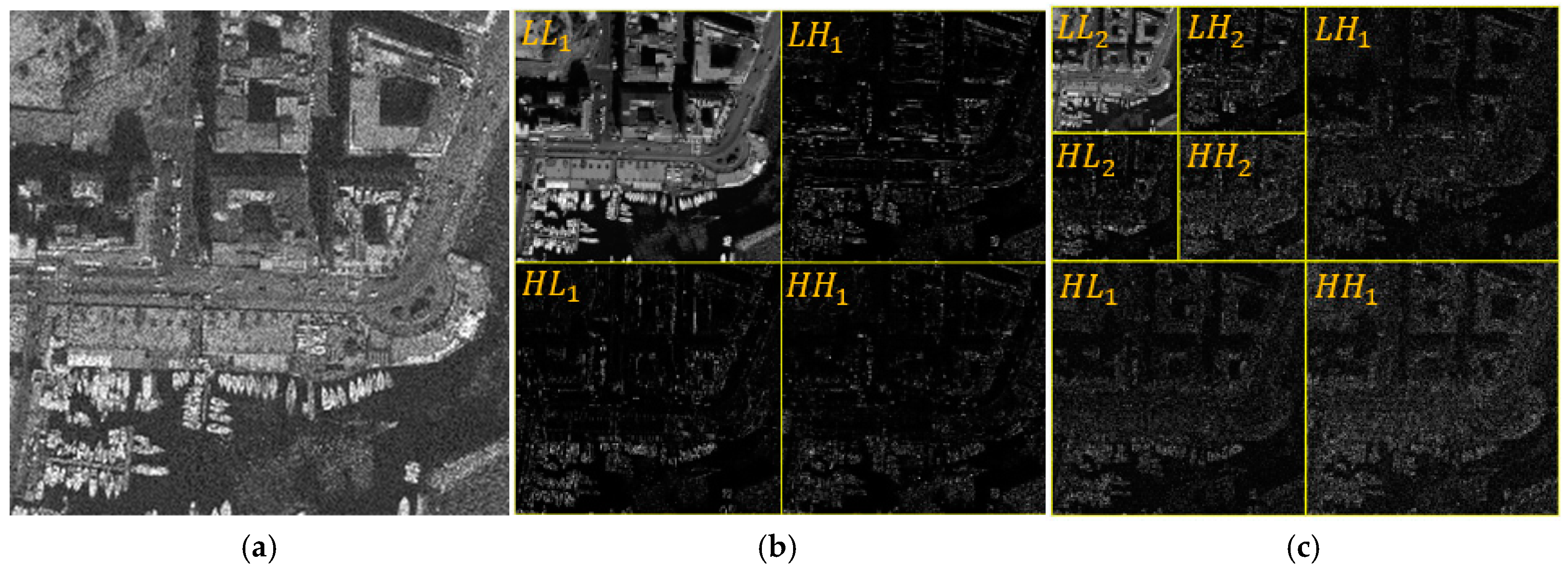
For the 2D image, the basic idea of the DWT is described, as follows. One-level DWT transforms the SAR images with speckle noise into four sub-band images: the approximate sub-band image () and three detailed sub-band images (vertical coefficients (), horizontal coefficients (), and diagonal coefficients ()) (Figure 2b). Figure 2c shows the results of the two-level wavelet decomposition. The two-level DWT decomposes the sub-band image that was obtained from the one-level wavelet decomposition in the same manner to obtain four sub-band images (, , , and ). The approximate sub-band image () contains the low-frequency coefficients, and detailed sub-band images (, , , , and ) depict the high-frequency coefficients. The detailed sub-band images present most information regarding the image, including the noise and edge information. The approximate sub-band image includes important information about the SAR images, such as the texture.
2.4. Soft Threshold
Various threshold methods exist ([32,33,34]). The most commonly used wavelet functions are the soft and hard threshold. These threshold methods are used to reduce the speckle noise in the SAR images. Although both thresholds set to zero when the coefficients are smaller than the threshold, these thresholds have the main difference. The former function suppresses the coefficients that are larger than the threshold, while the latter function leaves them unchanged [43].
The hard threshold removes the coefficients that are below the threshold value , as determined by the noise variance. The hard threshold is depicted, as follows:
where is the wavelet coefficient and is the threshold value. represents the wavelet coefficient after the hard threshold is applied. The hard threshold is known to have discontinuity in the noise-free image, since the wavelet coefficient at the threshold is suddenly zeroed. In the hard threshold method, the wavelet coefficients that do not exceed the given threshold value are zeroed. The other wavelet coefficients remain unchanged. Therefore, the hard threshold yields artifacts in the despeckled image [47]. The soft threshold applies the signum function in its model to overcome these issues of the hard threshold (Equation (13)).
Here, depicts the signum function. is the wavelet coefficient after the shrinkage of the soft threshold.
In the soft threshold method, the wavelet coefficients are zero if they are below the threshold. The wavelet coefficients above the threshold are shrunk by the threshold value. Hence, the soft threshold provides smooth results without artifacts. When compared to the hard threshold, the soft threshold generally exhibits excellent preservation of detail at the expense of computational complexity [43]. We apply the soft threshold to these sub-band images, since the horizontal and vertical sub-band images have a similar energy [48].
2.5. Guided Filter
Zhang and Gunturk [47] mentioned that noise may exist in the approximate sub-band image and detailed sub-band images in the wavelet domain. Gao et al. [43] have divided the 2D SAR images into low, medium, and high-frequency sub-band images using a 2D fast Fourier transform (FFT). The authors applied the approximate sub-band image through low-pass filtering to reduce the noise in the approximate sub-band image. This method shows low speckle noise removal and edge preservation ability. In [47,49], the authors applied the BF [13] to the approximate sub-band image to suppress speckle noise. BF is capable of preserving the edges and shows an excellent noise removal performance since it is difficult to distinguish between original signal and noise in the approximate sub-band image; however, it exhibits gradient distortion and high complexity [47]. We applied the GF [45] in the approximate sub-band image to overcome these problems. The process of removing the noise using the GF is as follows. GF models the output image for the guidance image of the window region with the center pixel in the image, as follows:
where and are linear coefficients estimated form the window . Equation (15) removes unwanted texture or noise to determine the linear coefficients.
Here, and denote the input image and noise component, respectively. The linear coefficients are obtained by Equation (16) to minimize the difference between the input image and the output image .
where is a normalization parameter that serves to prevent from becoming infinitely large. The minimization method of the liner coefficient in Equation (16) is as follows:
Here, and are the mean and variance of the guidance image in the window . represents the number of pixels in the mask , and . As the window size and adjust, the noise is removed and the edge areas are preserved. Therefore, these parameters are adjusted according to the characteristics of the approximate sub-band image to remove the additive noise and to preserve edge information.
2.6. Improved Guided Filter
2.6.1. A New Edge-Aware Weighting
The horizontal and vertical sub-band images of DWT have the same energy, while the diagonal sub-band image has lower energy at the same scale [48]. We propose new edge-aware weighting for effectively detecting and preserving weak edge information (Equation (19)). The gradient operator is an effective operator for detecting sharp edge regions in the image and protecting against unnecessary blurring phenomena around the edges. However, the gradient operator produces wide and blurred edges when the edge regions are not sharp. In contrast, since a Laplacian operator uses a second-order derivative operator that has a zero crossing level, it can detect the weak information of the edges while using the zero crossing level. Therefore, we can detect weak edges in the diagonal sub-band image in the wavelet domain.
Here, and are the Laplacian and Gradient operators, respectively. The value of is larger than 1 when is located at weak edges; however, it is smaller than 1 if is in the homogeneous regions.
2.6.2. The Proposed Filter
The new edge-aware weighting of Equation (19) is incorporated into the cost function of Equation (20). As mentioned above, an IGF obtains a solution that minimizes the input image and the output image , while maintaining the linear model of Equation (14). A cost function with applied new edge-ware weighting is expressed. as follows:
The optimal values of and are computed as:
The final value of is given as follows:
Here, and are the mean values of and within the window, respectively.
2.7. Evaluation Metrics
We used peak signal-to-noise (PSNR), structural similarity (SSIM), and equivalent number of looks (ENL) to compare the performance of speckle noise reduction in the SAR images [41]. The PSNR depicts the maximum signal-to-noise ratio. The PSNR is an objective measurement method that is used to evaluate image quality, and it is defined as follows:
where the mean square error (MSE) is given by:
where and represent the number of pixels in the vertical and horizontal directions of the image, respectively. is the pixel value at the position of the original image and is the pixel value at the coordinates of in the filtered image. The filtered image has a smaller MSE as the image approaches the original image . Larger PSNR values imply better noise reduction performances. The SSIM is an index that indicates the similarity between the original image and the filtered image . The SSIM is given, as follows:
Here, and are the mean values of and , respectively. and present the variance of and , respectively. is the covariance of and . and are the two variables used to stabilize the division that can occur with a weak denominator. When the value of SSIM is closer to 1, there is no difference between the original and the filtered image. The equivalent number of look (ENL) is used to evaluate the speckle noise reduction performance of the homogeneous regions in the image. It is a standard metric in the absence of reference images that is widely used to evaluate despeckling performance. The ENL is defined as:
where and are the estimated mean and standard deviation of the filtered SAR image. Larger ENL values indicate excellent speckle noise removal ability.
3. Experimental Results
3.1. Experiments on Standard Images
In this study, we selected 8-bit gray standard images (Airplane, Baboon, Barbara, Boat, Cameraman, Fruits, Hill, House, Lena, Man, Monarch, Napoli, Peppers, and Zelda) with 256 × 256, 512 × 512, and 748 × 512 pixels in order to evaluate the performance of speckle noise removal and edge preservation (Figure 3). Speckle noise ( was added to each image. The existing methods (NLM [14], Guided [45], Frost [50], Lee [51], Bitonic [52], weighted-least-squares (WLS) [53], non-local low-rank (NLLR) [54], anisotropic diffusion filter with memory based on speckle statistics (ADMSS) [55], SRAD [39], SRAD-Guided [56], SAR-BM3D [24]) and the proposed algorithm were used to compare the speckle noise suppression performance. Table 1 and Table 2 present the simulation conditions for the standard images. The optimal parameters of the SRAD-guided method are the same as those of the proposed algorithm (Table 2). The MATLAB 2018b software was used in a computer environment [Intel (R) Core (TM) i5-8500 CPU @ 3.0 GHz with 16 GB RAM].
Table 3 and Table 4 exhibit the PSNR (dB) and SSIM values of the despeckled standard images while using the existing filtering methods and the proposed algorithm. The best and second-best values among all of the despeckling methods are denoted in red and blue color, respectively. Table 3 reports the PSNR values of different filtering methods on the fourteen standard images. The SRAD filtering method exhibits the best speckle noise removal performance in the Baboon (PSNR = 23.52 dB) and Napoli (PSNR = 26.41 dB) images. The PSNR values of SAR-BM3D are quite similar to that of the proposed algorithm; however, SAR-BM3D in the Airplane, Barbara, Fruits, Hill, and House images exhibit slightly larger values of PSNR when compared with the proposed method. The PSNR values of the proposed algorithm show the best performance of speckle noise removal in the images (Boat = 27.55 dB; Cameraman = 26.87 dB; Lena = 30.13 dB; Man = 28.55 dB; Monarch = 29.64 dB; Peppers = 28.44 dB; and, Zelda = 32.77 dB) (Table 3).
In Table 4, the performances of the existing filtering methods and the proposed algorithm are compared in terms of SSIM. As aforementioned, the SRAD filtering technique provides the best edge preservation performance in two images (Baboon = 0.65 and Napoli = 0.77). In the Airplane, Barbara, Cameraman, Fruits, House, Lena, Monarch, and Zelda, SAR-BM3D provides the best edge preservation performance while the proposed algorithm exhibits the second-best performance (Airplane, Barbara, House, Lena, Monarch, and Zelda). The SAR-BM3D and the proposed method show the same edge preservation performance in Cameraman, Fruits, and Hill. The proposed algorithm shows the highest edge preservation performance in the following images: Boat = 0.73; Man = 0.77; and Peppers = 0.84. We confirm that the results obtained by the proposed algorithm, which is displayed in Table 3 and Table 4, demonstrate an excellent performance and rank at least second among the existing filtering techniques.
From Table 3 and Table 4, in the standard images, we analyze the performances of each method to evaluate the soft threshold, IGF, and GF in the wavelet domain (Table 5). In Baboon (PSNR = 22.69 (−0.83), SSIM = 0.60 (−0.05), Barbara (PSNR = 24.32 (−0.67), SSIM = 0.66 (−0.02)), Boat (PSNR = 27.23 (−0.14), SSIM = 0.70 (−0.01), Hill (PSNR = 28.06 (−0.19), SSIM = 0.72 (−0.01)), Man (PSNR = 28.14 (−0.17), SSIM = 0.75 (−0.01), and Napoli (PSNR = 25.72 (−0.69), SSIM = 0.75 (−0.02) images, it is confirmed that the noise reduction and the edge preservation performances are low when the soft threshold method is compared with the SRAD result image. In comparison with the SRAD result, only the edge preservation performance of the soft threshold has been improved in Airplane (PSNR = 26.94 (−0.03), SSIM = 0.73 (+0.01)) image. Cameraman (PSNR = 26.69 (−0.04), SSIM = 0.76 (0.00)), Fruits (PSNR = 27.44 (−0.01), SSIM = 0.76 (0.00)), Monarch (PSNR = 29.42 (−0.08), SSIM = 0.86 (0.86 (0.00), and Peppers (PNSR = 28.21 (−0.08), SSIM = 0.82 (0.00)) images have a low speckle noise removal and the same edge preservation performances. In the Lena (PSNR = 29,69 (0.00), SSIM = 0.81 (0.00)) and Zelda (PSNR = 32.67 (0.00), SSIM = 0.86 (0.00)) images, the soft threshold technique shows the same noise removal and edge preservation abilities as SRAD; the House (PSNR = 27.92 (+0.34), SSIM = 0.70 (−0.08)) image has only enhanced the noise suppression ability; however, it shows low edge preservation performance.
From Table 5, in the Man image, the IGF only exhibits reduced noise removal and the same edge preservation abilities (PSNR = 28.30 (−0.01), SSIM = 0.76). The Napoli (PSNR = 26.41, SSIM = 0.77) image has the same noise suppression and edge preservation performances. In the House (PSNR = 27.98 (+0.40), SSIM = 0.70 (−0.08)), enhanced noise reduction, and decreased edge preservation abilities are showed when the IGF method is applied. The IGF compared to the SRAD result image shows better noise suppression performance and the same edge preservation ability (Airplane (PSNR = 26.98 (+0.01), SSIM = 0.72), Baboon (PSNR = 23.53 (+0.01), SSIM = 0.65), Barbara (PSNR = 25.00 (+0.01), SSIM = 0.68), Boat (PSNR = 27.39 (+0.02), SSIM = 0.71), Cameraman (PSNR = 26.74 (+0.01), SSIM = 0.76), Hill (PSNR = 28.27 (+0.02), SSIM = 0.73), Lena (PSNR = 29.70 (+0.01), SSIM = 0.81), Monarch (PSNR = 29.51 (+0.01), SSIM = 0.86), Peppers (PSNR = 28.31 (+0.02), SSIM = 0.82), and Zelda (PSNR = 32.68 (+0.01), SSIM = 0.86) images). Fruits (PSNR = 27.46 (+0.01), SSIM = 0.78) image show enhanced noise reduction and edge preservation performances.
The result of comparing PSNR and SSIM values of GF and SRAD filtered images are as follows (Table 5): In the Napoli (PSNR = 26.39 (−0.02), SSIM = 0.78 (+0.01)) image, the noise reduction performance is reduced and the edge preservation ability is improved. The noise suppression performance is improved; however, the edge preservation ability is maintained in the House (PSNR = 28.64 (+1.06), SSIM = 0.78) and Zelda (PSNR = 32.78 (+0.11), SSIM = 0.86) images. In contrast, the Fruits image exhibits the same noise removal ability and enhanced edge preservation performance (PSNR = 27.45, SSIM = 0.78 (+0.02)). The Airplane, Baboon, Barbara, Boat, Cameraman, Hill, Lena, Man, Monarch, and Peppers images have an enhanced noise suppression and edge preservation performances (Airplane (PSNR = 27.48 (+0.51), SSIM = 0.82 (+0.10)), Baboon (PSNR = 23.78 (+0.26), SSIM = 0.66 (+0.01)), Barbara (PSNR = 25.30 (+0.31), SSIM = 0.71 (+0.03)), Boat (PSNR = 27.67 (+0.30), SSIM = 0.73 (+0.02)), Cameraman (PSNR = 26.91 (+0.17), SSIM = 0.80 (+0.04)), Hill (PSNR = 28.41 (+0.16), SSIM = 0.74 (+0.01)), Lena (PSNR = 29.72 (+0.03), SSIM = 0.82 (+0.01)), Man (PSNR = 28.52 (+0.21), SSIM = 0.77 (+0.01)), Monarch (PSNR = 29.71 (+0.21), SSIM = 0.89 (+0.03)), Peppers (PSNR = 28.38 (+0.09), SSIM = 0.84 (+0.02))).
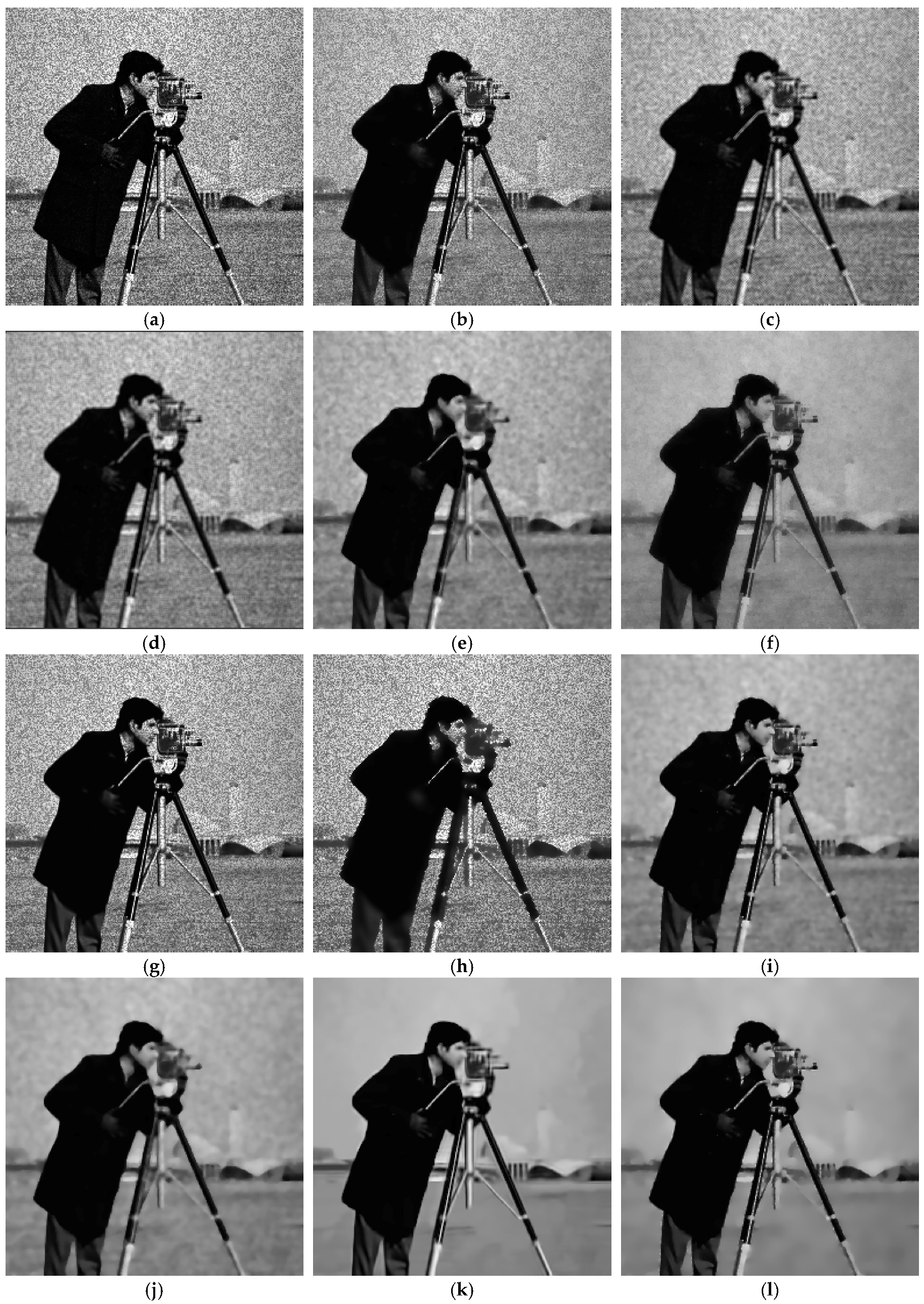
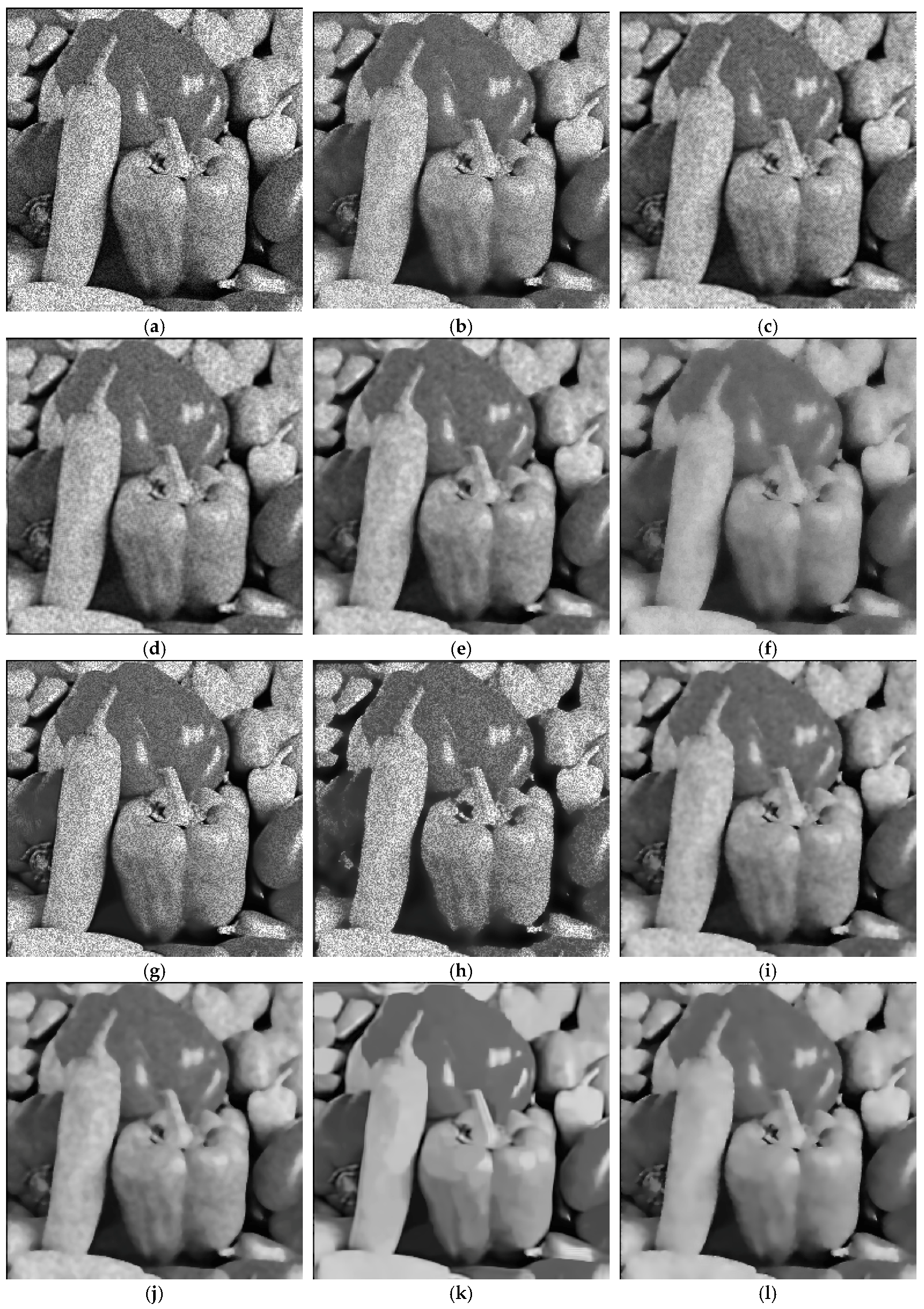
Figure 4, Figure 5 and Figure 6 show the despeckled images that are provided by existing filtering methods and the proposed algorithm for the standard images. Figure 4b–l, Figure 5b–l and Figure 6b–l exhibit the filtering result images of GF, Frost filter, Lee filter, Bitonic filter, WLS filter, NLLR method, ADMSS method, SRAD filter, SRAD-Guided algorithm, SAR-BM3D, and the proposed algorithm, respectively. In the Cameraman image, the issue of speckle noise residue in homogeneous regions appears in Figure 4b–e,g,h. Figure 4e, which is compared to Figure 4b–d,g,h exhibits reduced speckle noise but not quite. As shown in Figure 4f,i,j, some edges are lost in the edge regions, whereas the homogeneous regions remain with the speckle noise. The speckle noise reduction and edge preservation performance is noticeable in SAR-BM3D and the proposed algorithm (Figure 4k,l). The SAR-BM3D and the proposed algorithm exhibit similar performance with respect to the edge preservation, and show the strongest speckle removal ability in the homogeneous regions. However, the proposed algorithm has the best speckle noise removal performance in the homogeneous areas, as SAR-BM3D exhibits artifacts in these regions.
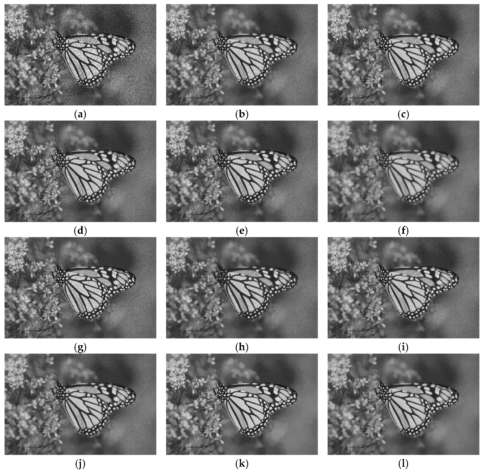
The GF, Frost filter, Lee filter, Bitonic filter, NLLR method, ADMSS method, and SRAD filter do not perform well for speckle noise removal in the homogeneous regions, and the speckle noise persists in the filtering result images (Figure 5b–e,g–i). The WLS filter and the SRAD-Guided algorithm perform better than the above filtering methods with regard to speckle noise reduction (Figure 5f,j). However, the WLS filter and the SRAD-Guided algorithm exhibit a blurring phenomenon in the image. The filtering result image that was obtained by the proposed algorithm had similar visual quality as SAR-BM3D. The SAR-BM3D achieves excellent edge preservation performance, however it exhibits artifacts in the homogeneous regions (Figure 5k). In Figure 5l, the proposed algorithm exhibits strong speckle noise removal ability while maintaining the edges. The qualitative result of Figure 5 represents the same result as in Figure 6.
3.2. Experiments on Real SAR Images
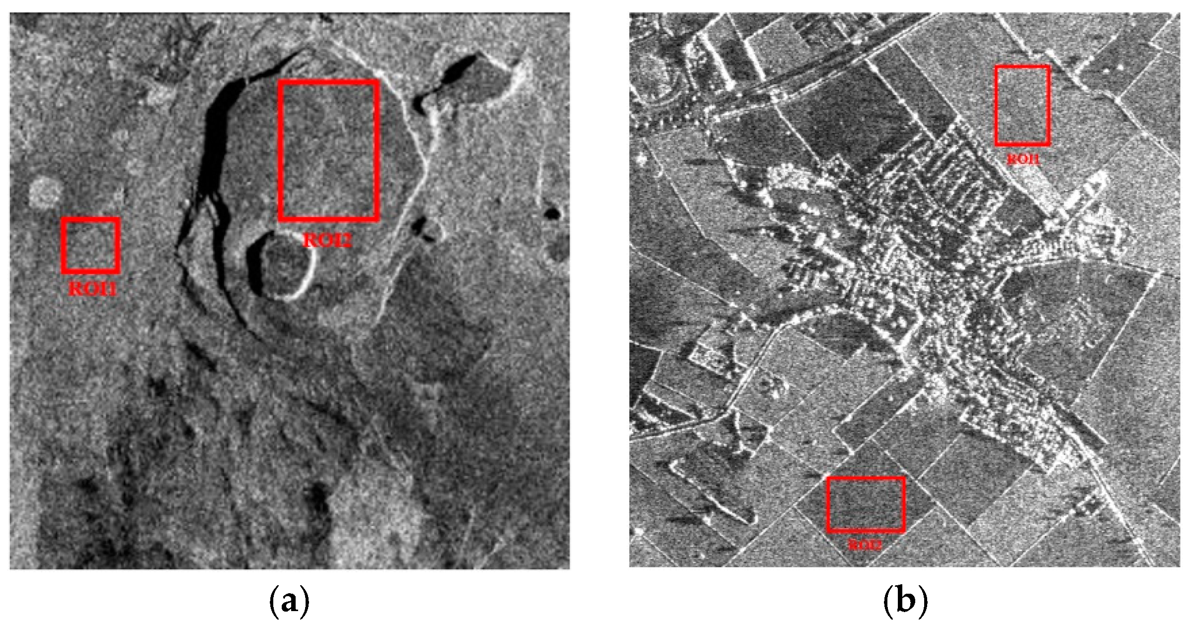
In this section, two real SAR images showing different scenes are used for the evaluation of the conventional filtering methods and the proposed algorithm on real SAR images (Figure 7). The real SAR image1 shows a scene from a photojournal [256 × 256, 8 bit, X-band] [57]. The real SAR image2 depicts a rural scene in Bedfordshire [512 × 512, 8 bit, X-band] [2,58]. As mentioned in Section 3.1, the optimal parameters of the conventional methods maintained the same values as those in the standard image (Table 1). Table 6 shows the optimal parameters of the proposed algorithm.
Table 7 and Table 8 list the ENL values that were computed in two regions of interest (ROIs) of the real SAR images. The GF in the ROI shows a low ENL value (SAR image1 (ENL1 = 17.89, ENL2 = 16.25), SAR image2 (ENL1 = 16.17, ENL2 = 13.13)), while the conventional filtering methods have better results, as shown in Table 7 and Table 8. According to Table 7, the NLM filter (ROI1 = 50.80, ROI2 = 40.87), Frost filter (ROI1 = 47.59, ROI2 = 37.85), Lee filter (ROI1 = 64.94, ROI2 = 49.15), Bitonic filter (ROI1 = 91.46, ROI2 = 64.98), NLLR method (ROI1 = 21.61, ROI2 = 19.41), ADMSS method (ROI1 = 18.59, ROI2 = 16.78), SRAD filter (ROI1 = 114.10, ROI2 = 81.01), and the SRAD-Guided method (ROI1 = 125.44, ROI2 = 88.88) do not exhibit excellent speckle noise removal performance in terms of the ENL. The SAR-BM3D (ROI1 = 135.16, ROI2 = 85.09), WLS (ROI1 = 165.71, ROI2 = 118.11), and proposed (ENL1 = 141.78, ENL2 = 99.92) methods show similar values of excellent speckle noise suppression ability. The SAR-BM3D, WLS, and proposed methods outperform the existing filtering methods, as implied by the higher ENL values were obtained by these methods in comparison to those of the existing filtering methods. Table 8 shows that the NLM filter (ROI1 = 29.53, ROI2 = 28.66), Frost filter (ROI1 = 48.47, ROI2 = 39.43), Lee filter (ROI1 = 62.14, ROI2 = 50.79), Bitonic filter (ROI1 = 99.30, ROI2 = 80.55), and NLLR method (ROI1 = 21.20, ROI2 = 20.56) have low speckle noise removal performances. The WLS (ROI1 = 207.56, ROI2 = 180.37), ADMSS (ROI1 = 201.56, ROI2 = 124.83), SRAD filter (ROI1 = 146.91, ROI2 = 117.17), SRAD-Guided (ROI1 = 174.02, ROI2 = 141.30), SAR- BM3D (ROI1 = 186.54, ROI2 = 129.35), and proposed (ROI1 = 205.89, ROI2 = 160.67) algorithms exhibit similar ENL values. Among these techniques, the WLS, ADMSS, and proposed methods represent a better ENL result when compared to the conventional filtering methods in speckle noise removal. Table 7 and Table 8 depict that the WLS filter outperforms all of the filtering methods in terms of the ENL, while the proposed method ranks second in the speckle noise suppression performance.
From Table 7 and Table 8, the data from Table 9 are analyzed for evaluating the performance of each method in the proposed method for the real SAR images. In the real SAR image1 and image2, the soft threshold, the IGF, and the GF methods, as compared to the SRAD filtering result image, shows enhanced noise suppression ability. In the SAR image1, the soft threshold, the IGF, and the GF techniques have enhanced noise removal ability (ROI-1 (ENL = 114.62 (+0.52)) and -2 (ENL = 81.59 (+0.58), ROI-1 (ENL = 118.84 (+4.74)) and -2 (ENL = 84.09 (+2.29), ROI-1 (ENL = 136.52 (+21.90)) and -2 (ENL = 97.05 (+16.04)). The noise reduction performance of the soft threshold (ROI-1 (ENL = 147.76 (+0.85)) and ROI-2 (ENL = 118.50 (+1.33)), IGF (ROI-1 (ENL = 148.93 (+2.02)) and ROI-2 (ENL = 119.27 (+2.10)), and the GF (ROI-1 (ENL = 203.02 (+56.11)) and ROI-2 (ENL = 157.24 (+40.07)) methods in the SAR image2 exhibits improved ability (Table 9).
Figure 8 shows the results of the simulated SAR images. Figure 8 shows that some filters, such as Guided, Frost, Lee, Bitonic, NLLR, and SRAD, do not exhibit strong speckle noise removal ability (Figure 8b–e,g,i). Table 6 and Table 7 illustrate that the WLS filter represents the best ENL value; however, it exhibits a blurring phenomenon in the image (Figure 8f). The SAR-guided method when compared with the SAR-BM3D and the proposed methods show inferior speckle noise removal and edge preservation performances. The SAR-BM3D method has an excellent speckle noise reduction and edge preservation abilities; however, artifacts in the homogeneous regions are observable (Figure 8k). The proposed algorithm compared with the SAR-BM3D method has a strong speckle noise removal ability; however, it does exhibit limited low edge preservation performance in some edge areas (Figure 8l).
3.3. Computational Complexity
Table 10 and Table 11 in this section present the time costs of the existing methods and the proposed algorithm on 14 standard images and two real SAR images. The experimental environments are those that are referred to in Section 3.1. Table 10 shows that the proposed method is much faster than Lee, NLLR, ADMSS, and SAR-BM3D. The running time of the proposed algorithm with 14 standard images is approximately 5.06 s on average. Table 11 denotes that the proposed algorithm has less computational complexity than the NLLR, ADMSS, and SAR-BM3D methods. The average execution time in the real SAR images is approximately 4.50 s.
Table 12 and Table 13 present the computing time of each step of the proposed method for the standard and real SAR images. The SRAD method has a high computing time, because the SRAD filter uses an iterative method to remove the speckle noise (standard images = 4.76 s (91.56%); SAR images = 4.12 s (91.56%)). In finding an optimal threshold value for classifying an original signal and a noise signal, the computing time of the soft threshold method is low, because, when compared to the computing time of the SRAD filter, it takes approximately 0.11 s (standard images) and 0.10 s (real SAR images). The IGF and the GF work very fast, because they only take approximately 6% (standard images) and 9% (real SAR images), respectively, of the total time. The main reason for this low time consumption is the use of a box filter in the GF [45]. The box filter can efficiently use a computational complexity in time by employing the integral image method [59]. The IGF is a method developed based on the GF; hence, it has a low computation time.
4. Discussion
This study used the statistical characteristics of speckle noise and the DWT to remove the speckle noise in SAR images. The proposed algorithm applies the SRAD filter, soft threshold, GF, and the IGF.
The speckle noise in SAR images is modelled as multiplicative noise. However, most of the filtering methods were developed for AWGN, as additive noise in imaging and sensing systems is most common. Therefore, conventional filtering methods are unable to remove speckle noise. The SRAD filtering method, in contrast, uses the ICOV to directly apply a diffusion process in all areas, except for the edge regions, by separating the edge areas and noise from SAR images with speckle noise. The SRAD filter exhibits excellent speckle noise removal and edge preservation. From the experimental results, the SRAD filtering scheme demonstrates the best speckle noise suppression and edge preservation performance among the single filtering methods. Based on this finding, the SRAD filtering technique was used as a preprocessing filter. In order to further remove the speckle noise remaining in the SRAD filtering result image, the logarithmic transform is used to convert the multiplicative noise (speckle noise) to additive noise. The SRAD filtering result image with the additive noise is decomposed into one low-frequency sub-band image () and six high-frequency sub-band images (, , , , and ) while using a two-level DWT. In the wavelet domain, horizontal (, ) and vertical (, ) sub-band images have the same energy, while, in comparison, the diagonal (, ) sub-band images have lower energies on the same scale. The former sub-band images were applied to soft threshold to remove the additive noise. The IGF method with new edge-aware weighting based on the Gradient and the Laplacian operators is applied to the latter sub-band images in order to remove the additive noise and preserve low edge information. We applied the guide filter to remove the additive noise that is present in the approximate () sub-band image. In some of the standard images, the proposed algorithm does not represent the best speckle noise removal and edge preservation performance in terms of PSNR and SSIM (Table 3 and Table 4). When the soft threshold, IGF, and GF are employed in the wavelet domain after the SRAD filter application in the proposed algorithm, when compared with the SRAD filter, the proposed algorithm shows enhanced speckle noise and edge preservation performance in the Airplane (PSNR = 0.48 dB; SSIM = 0.10), Boat (PSNR = 0.18 dB; SSIM = 0.02), Cameraman (PSNR = 0.14 dB; SSIM = 0.04), Lena (PSNR = 0.44 dB; SSIM = 0.02), Man (PSNR = 0.24 dB; SSIM = 0.01), Monarch (PSNR = 0.14 dB; SSIM = 0.03), Peppers (PSNR = 0.15 dB; SSIM = 0.02), and Zelda (PSNR = 0.15 dB; SSIM = 0.02) images. We analyzed the performance of each technique (soft threshold, IGF and GF) in the wavelet domain to achieve these results from standard images (Table 5). Among these methods, the soft threshold shows low speckle noise and edge preservation abilities in most standard images (average: PSNR = −0.19 dB; SSIM = −0.01). The IGF method exhibits a limited improvement in the speckle noise suppression performance (PSNR = +0.04 dB (avg.)). The GF technique contributes most of the speckle noise removal and edge preservation performances among each method in the wavelet domain (PSNR = +0.24 dB, SSIM = +0.02 (average)). When the same method that is applied in the standard images is applied to real SAR images, the proposed algorithm shows an improved speckle noise reduction performance in the ROI of the two real SAR images (SAR image1 (ROI-1: ENL = 27.68; ROI-2: ENL = 18.91) and SAR image2 (ROI-1: ENL = 58.98; ROI-2: ENL = 43.50)). From the ENL results in the real SAR images, we analyzed the contributions of the soft threshold, IGF, and GF to the noise suppression performance (Table 9). The soft threshold shows improved speckle noise rejection performance for ROI-1 (ENL = +0.69) and -2 (ENL = +0.85) in SAR image1 and 2. The IGF method exhibits enhanced speckle noise removal ability over the soft threshold (ROI-1 (ENL = +3.38) and ROI-2 (ENL = +2.20)). The GF technique was confirmed to have improved speckle noise reduction performance in terms of ENL = +39.27 at ROI-1 and ENL = +68.56 at ROI-2. The GF method has been found to have the greatest contribution to speckle noise removal in the wavelet domain.
The proposed algorithm shows the performance within the second-best value in all of the standard images and real SAR images in Table 3, Table 4, Table 7, and Table 8. The proposed method performs better than any nonlinear filter and hybrid method in the different images that have characteristics that include low-frequency components. Although the SAR-BM3D method, when compared to the conventional algorithms, exhibits excellent speckle noise reduction and edge preservation abilities, it employs noise reduction based on the NLM filter. The computational complexity of the SAR-BM3D algorithm is high, since the NLM filter needs to search regions. Therefore, it is difficult to obtain real time observations using the SAR-BM3D. The proposed algorithm exhibits a 10–30 times lower computational complexity when compared with SAR-BM3D (Table 10). In the proposed algorithm, the SRAD filter has a high computational complexity, because it uses an iterative method to remove the speckle noise (standard images = 4.76 s (91.56%); SAR images = 4.12 s (91.56%)); however, the time that is consumed by the soft threshold in finding an optimal value to classify an original signal and a noise signal is low (0.11 s (standard images) and 0.10 s (SAR images)). Moreover, the IGF and the GF have a low computational complexity (standard image 6%; real SAR images 9%), because the box filter in the IGF and the GF can efficiently employ computing time (). Moreover, the proposed method exhibits speckle noise suppression and edge preservation performance similarly to SAR-BM3D (Table 3 and Table 4). In the real SAR images, the WLS filter exhibits the best speckle noise removal performance in terms of ENL (Table 7 and Table 8). However, the resulting WLS image exhibits a blurring phenomenon (Figure 8f). As mentioned in [60], high ENL values do not always imply the best speckle noise suppression performance; further, blurring is observed in the image. Table 7 and Table 8 indicate that SAR-BM3D and the proposed method provide satisfactory speckle noise removal (Figure 8k,l). As mentioned above, the proposed algorithm has low computational complexity, which is about 8–13 times that of the SAR-BM3D method (Table 11). The experimental results demonstrate that the proposed method exhibits excellent speckle noise reduction, while preserving edge information and maintaining low computational complexity.
5. Conclusions
In summary, we proposed a novel algorithm that is based on statistical characteristics of speckle noise and the DWT to remove speckle noise from the SAR images. For this purpose, the SRAD filtering method, which can be directly applied to the SAR image, is used as a preprocessing filter. The logarithmic transform is employed to convert the multiplicative noise in the resulting SRAD image to additive noise. In order to further remove the additive noise from the SRAD filter result image, the two-level DWT converts the SRAD filter result image into one approximate sub-band image and six detailed sub-band images. The IGF is applied to diagonal sub-band images, which have lower energy within the same scale, to remove the additive noise and preserve edge information. Meanwhile, the horizontal and vertical sub-band images, which exhibit higher energy than the diagonal sub-band images, are treated with the soft threshold. The GF is applied to remove the additive noise that is present in the approximate sub-band image. The experiments in this study used both standard images and real SAR images. The experimental results demonstrate that the proposed method is able to obtain excellent speckle noise removal and edge preservation at low computational complexity when compared with the state-of-the art methods. In future research, we aim to study a novel filtering technique that can remove noise while preserving edge information in the approximate sub-band image.
Author Contributions
H.C. designed the methodology, implemented the simulation, and wrote this paper. J.J. wrote and edited this paper.
Funding
This research was not funded.
Acknowledgments
The authors would like to thank the reviewers’ for their good suggestions.
Conflicts of Interest
The authors declare no conflict of interest.
References
- Yahya, N.; Karmel, N.S.; Malik, A.S. Subspace-Based Technique for Speckle Noise Reduction in SAR Images. IEEE Trans. Geosci. Remote Sens. 2014, 52, 6257–6271. [Google Scholar] [CrossRef]
- Liu, F.; Wu, J.; Li, L.; Jiao, L.; Hao, H.; Zhang, X. A Hybrid Method of SAR Speckle Reduction Based on Geometric-Structural Block and Adaptive Neighborhood. IEEE Trans. Geosci. Remote Sens. 2018, 56, 730–747. [Google Scholar] [CrossRef]
- Guo, F.; Zhang, G.; Zhang, Q.; Zhao, R.; Deng, M.; Xu, K. Speckle Suppression by Weighted Euclidean Distance Anisotropic Diffusion. Remote Sens. 2018, 10, 722. [Google Scholar] [CrossRef]
- Yuan, Q.; Zhang, Q.; Li, J.; Shen, H.; Zhang, L. Hyperspectral image denoising employing a spatial-spectral deep residual convolutional neural network. IEEE Trans. Geosci. Remote Sens. 2018, 57, 1205–1218. [Google Scholar] [CrossRef]
- Zhang, Q.; Yuan, Q.; Zeng, C.; Wei, X.; Wei, Y. Missing data reconstruction in remote sensing image with a unified spatial-temporal-spectral deep convolutional neural network. IEEE Trans. Geosci. Remote Sens. 2018, 56, 4274–4288. [Google Scholar] [CrossRef]
- Yuan, Y.; Fang, J.; Lu, X.; Feng, Y. Remote sensing image scene classification using rearranged local features. IEEE Trans. Geosci. Remote Sens. 2018, 57, 1779–1792. [Google Scholar] [CrossRef]
- Tu, B.; Zhang, X.; Kang, X.; Zhang, G.; Li, S. Density peak-based noisy label detection for hyperspectral image classification. IEEE Trans. Geosci. Remote Sens. 2019, 57, 1573–1584. [Google Scholar] [CrossRef]
- Gemme, L.; Dellepiane, S.G. An automatic data-driven method for SAR image segmentation in sea surface analysis. IEEE Trans. Geosci. Remote Sens. 2018, 56, 2633–2646. [Google Scholar] [CrossRef]
- Duan, Y.; Liu, F.; Jiao, L.; Tao, X.; Wu, J.; Shi, C.; Wimmers, M.O. Adaptive hierarchical multinomial latent model with hybrid kernel function for SAR image semantic segmentation. IEEE Trans. Geosci. Remote Sens. 2018, 56, 5997–6015. [Google Scholar] [CrossRef]
- Liu, S.; Wu, G.; Zhang, X.; Zhang, K.; Wang, P.; Li, Y. SAR despeckling via classification-based nonlocal and local sparse representation. Neurocomputing 2017, 219, 174–185. [Google Scholar] [CrossRef]
- Xie, H.; Pierce, L.E.; Ulaby, F.T. Statistical properties of logarithmically transformed speckle. IEEE Trans. Geosci. Remote Sens. 2002, 40, 721–727. [Google Scholar] [CrossRef]
- Barash, D. A fundamental relationship between bilateral filtering, adaptive smoothing and the nonlinear diffusion equation. IEEE Trans. Pattern Anal. Machine Intell. 2002, 24, 844–867. [Google Scholar] [CrossRef]
- Tomasi, C.; Manduchi, R. Bilateral Filtering for Gray and Color Images. In Proceedings of the Sixth International Conference on Computer Vision, Bombay, India, 4–7 January 1998; pp. 839–846. [Google Scholar]
- Buades, A.; Coll, B.; Morel, J.-M. A non-local algorithm for image denoising. In Proceedings of the 2005 IEEE Computer Society Conference on Computer Vision and Pattern Recognition, San Diego, CA, USA, 20–25 June 2005; pp. 60–65. [Google Scholar]
- Buades, A.; Coll, B.; Morel, J.M. A review of image denoising algorithms, with a new one. SIAM Multiscale Model. Simul. 2005, 490–530. [Google Scholar] [CrossRef]
- Torres, L.; Sant’Anna, S.J.S.; Freitas, C.D.C.; Frery, C. Speckle reduction in polarimetric SAR imagery with stochastic distances and nonlocal means. Pattern Recognit. 2014, 141–157. [Google Scholar] [CrossRef]
- Xu, W.; Tang, C.; Gu, F.; Cheng, J. Combination of oriented partial differential equation and shearlet transform for denoising in electronic speckle pattern interferometry fringe patters. Appl. Opt. 2017, 56, 2843–2850. [Google Scholar] [CrossRef] [PubMed]
- Perona, P.; Malik, J. Scale-Space and Edge Detection Using Anisotropic Diffusion. IEEE Trans. Pattern Anal. Mach. Intell. 1990, 12, 629–639. [Google Scholar] [CrossRef]
- Li, J.C.; Ma, Z.H.; Peng, Y.X.; Huang, H. Speckle reduction by image entropy anisotropic diffusion. Acta Phys. Sin. 2013, 62, 099501. [Google Scholar]
- Deledalle, C.A.; Denis, L.; Tupin, F. Iterative weighted maximum likelihood denoising with probabilistic patch-based weights. IEEE Trans. Image Process. 2009, 18, 2661–2672. [Google Scholar] [CrossRef]
- Zhang, J.; Lin, G.; Wu, L.; Cheng, Y. Speckle filtering of medical ultrasonic images using wavelet and guided filter. Ultrasonics 2016, 65, 177–193. [Google Scholar] [CrossRef] [PubMed]
- Su, X.; Deledalle, C.; Tupin, F.; Sun, F. Two-step multitemporal nonlocal means for synthetic aperture radar images. IEEE Trans. Geosci. Remote Sens. 2014, 52, 6181–6196. [Google Scholar]
- Chierchia, C.; Mirelle, E.G.; Scarpa, G.; Verdoliva, L. Multitemporal SAR image despeckling based on block-matching and collaborative filtering. IEEE Trans. Geosci. Remote Sens. 2017, 55, 5467–5480. [Google Scholar] [CrossRef]
- Parrilli, S.; Poderico, M.; Angelino, C.V.; Verdoliva, L. A nonlocal SAR image denoising algorithm based on LLMMSE wavelet shrinkage. IEEE Trans. Geosci. Remote Sens. 2012, 50, 606–616. [Google Scholar] [CrossRef]
- Wu, M.-T. Wavelet transform based on Meyer algorithm for image edge and blocking artifact reduction. Inf. Sci. 2019, 474, 125–135. [Google Scholar] [CrossRef]
- Singh, R.; Khare, A. Fusion of multimodal medical images using Daubechies complex wavelet transform—A multiresolution approach. Inform. Fusion 2014, 19, 49–60. [Google Scholar] [CrossRef]
- Li, H.; Manjunath, B.S.; Mitra, S.K. Multisensor image fusion using the wavelet transform. Graph. Models Image Process. 1995, 57, 235–245. [Google Scholar] [CrossRef]
- Pajares, G.; de la Cruz, J.M. A wavelet-based image fusion tutorial. Pattern Recognit. 2004, 37, 1855–1872. [Google Scholar] [CrossRef]
- Huang, Z.-H.; Li, W.-J.; Wang, J.; Zhang, T. Face recognition based on pixel-level and feature-level fusion of the top-level’s wavelet sub-bands. Inf. Fusion 2015, 22, 95–104. [Google Scholar] [CrossRef]
- Hsia, C.-H.; Guo, J.-M. Efficient modified directional lifting-based discrete wavelet transform for moving object detection. Signal Process. 2014, 96, 138–152. [Google Scholar] [CrossRef]
- Liu, S.; Florencio, D.; Li, W.; Zhao, Y.; Cook, C. A Fusion Framework for Camouflaged Moving Foreground Detection in the Wavelet Domain. IEEE Trans. Image Process. 2018, 27, 3918–3930. [Google Scholar] [CrossRef]
- Donoho, D.L. De-noising by soft-thresholding. IEEE Trans. Inf. Theory 1995, 25, 613–627. [Google Scholar] [CrossRef]
- Donoho, D.L.; Johnstone, I.M. Adapting to unknown smoothness via wavelet shrinkage. J. Am. Stat. Assoc. 1995, 90, 1200–1224. [Google Scholar] [CrossRef]
- Chang, S.G.; Yu, B.; Vetterli, M. Adaptive wavelet thresholding for image denoising and compression. IEEE Trans. Image Process. 2000, 9, 1532–1546. [Google Scholar] [CrossRef] [Green Version]
- Yang, Y.; Ding, Z.; Liu, J.; Gao, Q.; Yuan, X.; Lu, X. An adaptive SAR image speckle noise algorithm based on wavelet transform and diffusion equations for marine scenes. In Proceedings of the 2017 IEEE International Geoscience and Remote Sensing Symposium, Fort Worth, TX, USA, 23–28 July 2017; pp. 1–4. [Google Scholar]
- Amini, M.; Ahmad, M.O.; Swamy, M.N.S. SAR image despeckling using vector-based hidden markov model in wavelet domain. In Proceedings of the 2016 IEEE Canadian Conference on Electrical and Computer Engineering, Vancouver, BC, Canada, 15–18 May 2016; pp. 1–4. [Google Scholar]
- Li, H.-C.; Hong, W.H.; Wu, Y.-R.; Fan, P.-Z. Bayesian Wavelet Shrinkage with Heterogeneity-Adaptive Threshold for SAR images despeckling based on Generalized Gamma Distribution. IEEE Trans. Geosci. Remote Sens. 2013, 51, 2388–2402. [Google Scholar] [CrossRef]
- Rajesh, M.R.; Mridula, S.; Mohanan, P. Speckle Noise Reduction in Images using Wiener Filtering and Adaptive Wavelet Thresholding. In Proceedings of the 2016 IEEE Region 10 Conference (TENCON), Singapore, 22–25 November 2016; pp. 2860–2863. [Google Scholar]
- Yu, Y.; Acton, S.T. Speckle reducing anisotropic diffusion. IEEE Trans. Image Process. 2002, 11, 1260–1270. [Google Scholar] [PubMed] [Green Version]
- Dass, R. Speckle noise reduction of ultrasound images using BFO cascaded with wiener filter and discrete wavelet transform in homomorphic region. Procedia Comput. Sci. 2018, 132, 1543–1551. [Google Scholar] [CrossRef]
- Singh, P.; Shree, R. A new SAR image despeckling using directional smoothing filter and method noise thresholding. Eng. Sci. Technol. Int. J. 2019, 21, 589–610. [Google Scholar] [CrossRef]
- Choi, H.H.; Lee, J.H.; Kim, S.M.; Park, S.Y. Speckle noise reduction in ultrasound images using a discrete wavelet transform-based image fusion technique. Biomed. Mater. Eng. 2015, 26, 1587–1597. [Google Scholar] [CrossRef] [PubMed]
- Gao, F.; Xue, X.; Sun, J.; Wang, J.; Zhang, Y. A SAR Image Despeckling Method Based on Two-Dimensional S Transform Shrinkage. IEEE Trans. Geosci. Remote Sens. 2016, 54, 3025–3034. [Google Scholar] [CrossRef]
- Sivaranjania, R.; Roomi, S.M.M.; Senthilarasi, M. Speckle noise removal in SAR images using Multi-Objective PSO (MOPSO) algorithm. Appl. Soft Comput. 2019, 76, 671–681. [Google Scholar] [CrossRef]
- He, K.; Sun, J.; Tang, X. Guided image filtering. IEEE Trans. Pattern Anal. Mach. Intell. 2013, 35, 1397–1409. [Google Scholar] [CrossRef]
- Saevarsson, B.B.; Sveinsson, J.R.; Benediktsson, J.A. Combined Wavelet and Curvelet Denoising of SAR Images. In Proceedings of the 2007 IEEE International Geoscience and Remote Sensing Symposium, Barcelona, Spain, 23–28 July 2007; pp. 4235–4238. [Google Scholar]
- Zhang, M.; Gunturk, B.K. Multiresolution Bilateral Filtering for Image Denoising. IEEE Trans. Image Process. 2008, 17, 2324–2333. [Google Scholar] [CrossRef] [Green Version]
- Sheikh, H.R.; Bovik, A.C.; Cormack, L. No-reference Quality Assessment Using Natural Scene Statistics: JPEG2000. IEEE Trans. Image Process. 2005, 14, 1918–1927. [Google Scholar] [CrossRef] [PubMed]
- Wenxuan, S.; Jie, L.; Minyuan, W. An image denoising method based on multiscale wavelet thresholding and bilateral filtering. Wuhan Univ. J. Nat. Sci. 2010, 15, 148–152. [Google Scholar]
- Frost, V.S.; Stiles, J.A.; Shanmugan, K.S.; Holtzman, J.C. A model for radar images and its application to adaptive digital filtering of multiplicative noise. IEEE Trans. Pattern Anal. Mach. Intell. 1982, PAMI-4, 66–157. [Google Scholar] [CrossRef]
- Lee, S.T. Digital image enhancement and noise filtering by use of local statistics. IEEE Trans. Pattern Anal. Mach. Intell. 1980, PAMI-2, 165–168. [Google Scholar] [CrossRef]
- Treece, G. The bitonic filter: Linear filtering in an edge-preserving morphological framework. IEEE Trans. Image Process. 2016, 25, 5199–5211. [Google Scholar] [CrossRef] [PubMed]
- Farbman, Z.; Fattal, R.; Lischinski, D.; Szeliski, R. Edge-preserving decomposition for multi-scale tone and detail manipulation. ACM Trans. Graph. 2008, 27. [Google Scholar] [CrossRef]
- Zhu, L.; Fu, C.-W.; Brown, M.S.; Heng, P.-A. A non-local low-rank framework for ultrasound speckle reduction. In Proceedings of the 2017 IEEE Conference on Computer Vision and Pattern Recognition, Honolulu, HI, USA, 21–26 July 2017; pp. 5650–5658. [Google Scholar]
- Ramos-Llordén, G.; Vegas-Sánchez-Ferrero, G.; Martin-Fernández, M.; Alberola-López, C.; Aja-Fernández, S. Anisotropic diffusion filter with memory based on speckle statistics for ultrasound images. IEEE Trans. Image Process. 2015, 24, 345–358. [Google Scholar] [CrossRef]
- Hyunho, C.; Jechang, J. Speckle noise reduction in ultrasound images using SRAD and guided filter. In Proceedings of the International Workshop on Advanced Image Technology, Chiang Mai, Thailand, 7–9 January 2018; pp. 1–4. [Google Scholar]
- Jet Propulsion Laboratory. Available online: https://photojournal.jpl.nasa.gov/catalog/PIA01763 (accessed on 30 December 2018).
- Dataset of Standard 512X512 Grayscale Test Images. Available online: http://decsai.ugr.es/cvg/CG/base.htm (accessed on 30 December 2018).
- Crow, F. Summed-area tables for texture mapping. In Proceedings of the 11th Annual Conference on Computer Graphics and Interactive Techniques, New York, NY, USA, 1984; pp. 207–212. [Google Scholar]
- Elad, M.; Ahalon, M. Image denoising via learned dictionaries and sparse representation. In Proceedings of the 2006 IEEE Computer Society Conference on Computer Vision and Pattern Recognition, New York, NY, USA, 17–22 June 2006; pp. 895–900. [Google Scholar]
Figure 1.
Block diagram of the proposed algorithm.

Figure 2.
Two-dimensional (2D) image decomposition result by different discrete wavelet transform (DWT) levels. (a) Image of Napoli; (b) One-level wavelet decomposition; and, (c) Two-level wavelet decomposition.
Figure 2.
Two-dimensional (2D) image decomposition result by different discrete wavelet transform (DWT) levels. (a) Image of Napoli; (b) One-level wavelet decomposition; and, (c) Two-level wavelet decomposition.

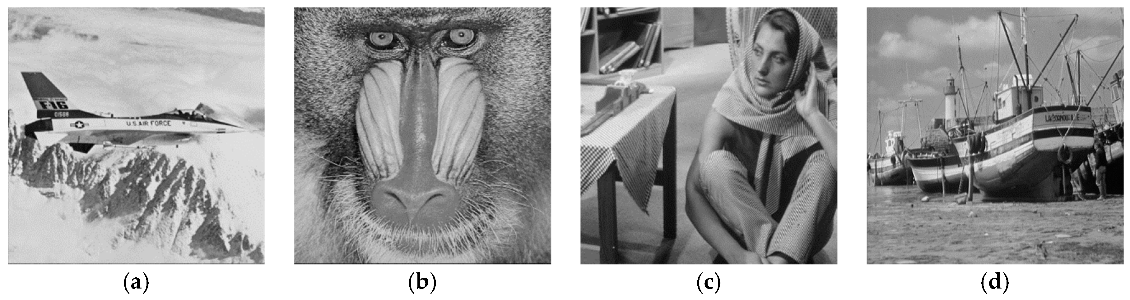
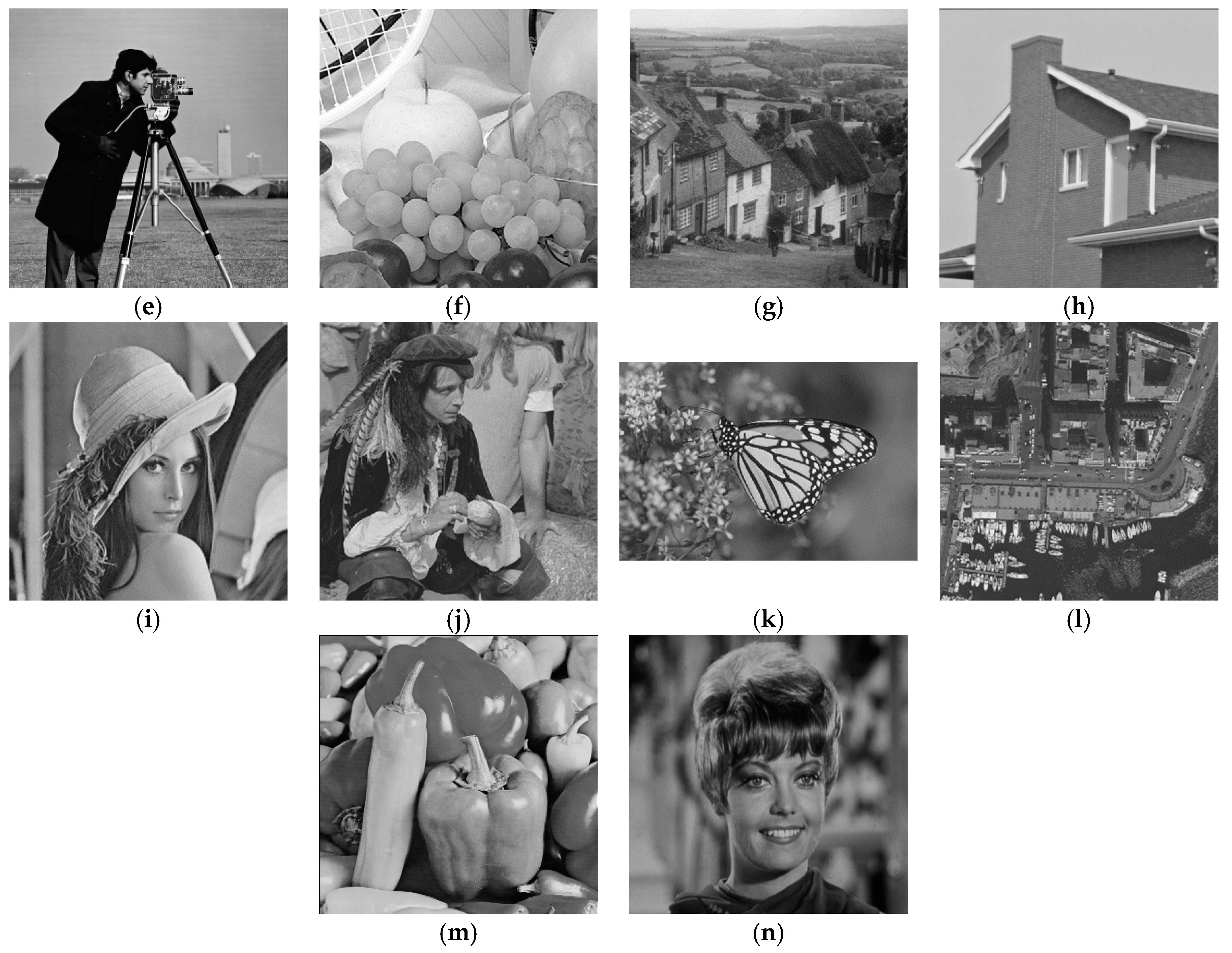
Figure 3.
Images used in the experiments. (a) Airplane (512 × 512); (b) Baboon (512 × 512); (c) Barbara (512 × 512); (d) Boat (512 × 512); (e) Cameraman (256 × 256); (f) Fruits (512 × 512); (g) Hill (512 × 512); (h) House (256 × 256); (i) Lena (512 × 512); (j) Man (512 × 512); (k) Monarch (748 × 512); (l) Napoli (512 × 512); (m) Peppers (256 × 256); and, (n) Zelda (512 × 512).


Figure 4.
Performance comparison of different techniques in Cameraman image. (a) Noisy; (b) Guided; (c) Frost; (d) Lee; (e) Bitonic; (f) weighted-least-squares (WLS); (g) non-local low-rank (NLLR); (h) anisotropic diffusion filter with memory based on speckle statistics (ADMSS); (i) speckle reducing anisotropic diffusion (SRAD); (j) SRAD-Guided; (k) SAR-BM3D; and, (l) Proposed algorithm.

Figure 5.
Performance comparison of different techniques in Monarch image. (a) Noisy; (b) Guided; (c) Frost; (d) Lee; (e) Bitonic; (f) WLS; (g) NLLR; (h) ADMSS; (i) SRAD; (j) SRAD-Guided; (k) SAR-BM3D; and, (l) Proposed algorithm.
Figure 5.
Performance comparison of different techniques in Monarch image. (a) Noisy; (b) Guided; (c) Frost; (d) Lee; (e) Bitonic; (f) WLS; (g) NLLR; (h) ADMSS; (i) SRAD; (j) SRAD-Guided; (k) SAR-BM3D; and, (l) Proposed algorithm.

Figure 6.
Performance comparison of different techniques in Peppers image. (a) Noisy; (b) Guided; (c) Frost; (d) Lee; (e) Bitonic; (f) WLS; (g) NLLR; (h) ADMSS; (i) SRAD; (j) SRAD-Guided; (k) SAR-BM3D; and, (l) Proposed algorithm.
Figure 6.
Performance comparison of different techniques in Peppers image. (a) Noisy; (b) Guided; (c) Frost; (d) Lee; (e) Bitonic; (f) WLS; (g) NLLR; (h) ADMSS; (i) SRAD; (j) SRAD-Guided; (k) SAR-BM3D; and, (l) Proposed algorithm.


Figure 8.
Performance comparison of different techniques in SAR image2. (a) Noisy; (b) Guided; (c) Frost; (d) Lee; (e) Bitonic; (f) WLS; (g) NLLR; (h) ADMSS; (i) SRAD; (j) SRAD-Guided; (k) SAR-BM3D; and, (l) Proposed algorithm.
Figure 8.
Performance comparison of different techniques in SAR image2. (a) Noisy; (b) Guided; (c) Frost; (d) Lee; (e) Bitonic; (f) WLS; (g) NLLR; (h) ADMSS; (i) SRAD; (j) SRAD-Guided; (k) SAR-BM3D; and, (l) Proposed algorithm.


Table 1.
Optimal parameters of the existing methods in the standard images.
| Methods | Optimal Parameters |
|---|---|
| NLM | Mask size = 3 × 3 |
| Frost | Mask size = 3 × 3 |
| Lee | Mask size = 3 × 3 |
| Bitonic | Mask size = 3 × 3 |
| WLS | Mask size = 3 × 3, = 3 |
| NLLR | = 10, H = 10 |
| ADMSS | = 0.5, = 0.1, = 15 |
| SAR-BM3D | Number of rows/cols of block = 9, Maximum size of the 3rd dimension of a stack = 16, Diameter of search area = 39, Dimension of step = 3, Parameter of the 2D Kaiser window = 2, Transform UDWT = daub4 |
Table 2.
Optimal parameters of the proposed method in the standard images.
| SRAD Filter | IGF | GF | |
|---|---|---|---|
| Airplane | Time step = 0.01 Exponential decay rate = 1 Number of iterations = 115 | Mask size = 33 × 33 Regularization parameter = 0.0001 | Mask size = 3 × 3 Regularization parameter = 0.001 |
| Baboon | Time step = 0.01 Exponential decay rate = 1 Number of iterations = 50 | Mask size = 5 × 5 Regularization parameter = 1e−10 | Mask size = 3 × 3 Regularization parameter = 0.001 |
| Barbara | Time step = 0.01 Exponential decay rate = 1 Number of iterations = 70 | Mask size = 3 × 3 Regularization parameter = 1e−10 | Mask size = 3 × 3 Regularization parameter = 0.001 |
| Boat | Time step = 0.01 Exponential decay rate = 1 Number of iterations = 100 | Mask size = 3 × 3 Regularization parameter = 1e−10 | Mask size = 3 × 3 Regularization parameter = 0.001 |
| Cameraman | Time step = 0.01 Exponential decay rate = 1 Number of iterations = 200 | Mask size = 3 × 3 Regularization parameter = 1e−10 | Mask size = 3 × 3 Regularization parameter = 0.001 |
| Fruits | Time step = 0.01 Exponential decay rate = 1 Number of iterations = 150 | Mask size = 17 × 17 Regularization parameter = 0.01 | Mask size = 3 × 3 Regularization parameter = 0.001 |
| Hill | Time step = 0.01 Exponential decay rate = 1 Number of iterations = 100 | Mask size = 17 × 17 Regularization parameter = 1e−10 | Mask size = 3 × 3 Regularization parameter = 0.001 |
| House | Time step = 0.01 Exponential decay rate = 1 Number of iterations = 190 | Mask size = 3 × 3 Regularization parameter = 1e−10 | Mask size = 3 × 3 Regularization parameter = 0.001 |
| Lena | Time step = 0.01 Exponential decay rate = 1 Number of iterations = 150 | Mask size = 17 × 17 Regularization parameter = 0.01 | Mask size = 3 × 3 Regularization parameter = 0.001 |
| Man | Time step = 0.01 Exponential decay rate = 1 Number of iterations = 100 | Mask size = 17 × 17 Regularization parameter = 0.01 | Mask size = 3 × 3 Regularization parameter = 0.001 |
| Monarch | Time step = 0.01 Exponential decay rate = 1 Number of iterations = 100 | Mask size = 3 × 3 Regularization parameter = 1e−10 | Mask size = 3 × 3 Regularization parameter = 0.001 |
| Napoli | Time step = 0.01 Exponential decay rate = 1 Number of iterations = 80 | Mask size = 3 × 3 Regularization parameter = 1e−10 | Mask size = 3 × 3 Regularization parameter = 0.001 |
| Peppers | Time step = 0.01 Exponential decay rate = 1 Number of iterations = 120 | Mask size = 3 × 3 Regularization parameter = 1e−10 | Mask size = 3 × 3 Regularization parameter = 0.001 |
| Zelda | Time step = 0.01 Exponential decay rate = 1 Number of iterations = 140 | Mask size = 3 × 3 Regularization parameter = 1e−10 | Mask size = 3 × 3 Regularization parameter = 0.001 |
Table 3.
Peak signal-to-noise (PSNR) (in dB) results for each standard image.
| Noisy | NLM | Guided | Frost | Lee | Bitonic | WLS | NLLR | ADMSS | SRAD | SRAD-Guided | SAR-BM3D | Proposed | |
|---|---|---|---|---|---|---|---|---|---|---|---|---|---|
| Airplane | 16.53 | 19.12 | 19.14 | 22.06 | 23.78 | 26.18 | 24.97 | 17.39 | 23.43 | 26.97 | 26.53 | 28.10 | 27.45 |
| Baboon | 18.49 | 21.13 | 21.09 | 21.08 | 21.91 | 21.97 | 22.12 | 19.53 | 18.28 | 23.52 | 22.07 | 22.51 | 22.92 |
| Barbara | 19.16 | 22.40 | 22.05 | 22.34 | 23.26 | 23.68 | 23.78 | 20.39 | 20.50 | 24.99 | 23.75 | 28.32 | 24.59 |
| Boat | 18.46 | 21.81 | 21.68 | 23.36 | 19.41 | 26.39 | 25.50 | 19.65 | 20.14 | 27.37 | 26.59 | 27.20 | 27.55 |
| Camera-man | 18.66 | 21.65 | 21.59 | 22.41 | 22.85 | 24.43 | 25.03 | 19.75 | 17.59 | 26.73 | 24.71 | 26.35 | 26.87 |
| Fruits | 17.08 | 19.96 | 19.98 | 22.30 | 24.08 | 26.33 | 26.31 | 18.04 | 22.07 | 27.45 | 26.93 | 27.68 | 27.45 |
| Hill | 19.79 | 23.54 | 23.38 | 24.64 | 25.48 | 27.58 | 26.75 | 21.26 | 24.92 | 28.25 | 27.82 | 28.30 | 28.27 |
| House | 17.93 | 21.16 | 21.02 | 23.26 | 25.06 | 27.38 | 25.93 | 19.09 | 22.46 | 27.58 | 27.81 | 29.83 | 28.58 |
| Lena | 18.84 | 22.45 | 22.31 | 24.29 | 25.88 | 28.54 | 27.39 | 20.11 | 21.88 | 29.69 | 28.99 | 29.91 | 30.13 |
| Man | 19.51 | 23.07 | 22.94 | 24.41 | 26.15 | 27.46 | 26.46 | 20.83 | 20.82 | 28.31 | 27.68 | 27.71 | 28.55 |
| Monarch | 20.19 | 24.55 | 24.10 | 25.11 | 26.76 | 27.70 | 25.87 | 21.99 | 24.00 | 29.50 | 28.03 | 29.54 | 29.64 |
| Napoli | 21.00 | 24.62 | 24.27 | 24.06 | 24.48 | 24.34 | 23.69 | 22.71 | 22.90 | 26.41 | 24.34 | 25.14 | 25.70 |
| Peppers | 18.74 | 22.05 | 21.79 | 23.50 | 22.92 | 26.62 | 25.77 | 19.96 | 18.13 | 28.29 | 27.22 | 27.13 | 28.44 |
| Zelda | 21.18 | 26.23 | 25.94 | 26.71 | 28.62 | 31.40 | 30.66 | 23.19 | 29.28 | 32.67 | 32.20 | 32.38 | 32.77 |
Table 4.
Structural similarity (SSIM) results for each standard image.
| Noisy | NLM | Guided | Frost | Lee | Bitonic | WLS | NLLR | ADMSS | SRAD | SRAD-Guided | SAR-BM3D | Proposed | |
|---|---|---|---|---|---|---|---|---|---|---|---|---|---|
| Airplane | 0.21 | 0.29 | 0.28 | 0.37 | 0.50 | 0.66 | 0.70 | 0.25 | 0.73 | 0.72 | 0.76 | 0.84 | 0.82 |
| Baboon | 0.49 | 0.56 | 0.56 | 0.47 | 0.54 | 0.52 | 0.53 | 0.53 | 0.39 | 0.65 | 0.53 | 0.56 | 0.61 |
| Barbara | 0.44 | 0.61 | 0.57 | 0.50 | 0.60 | 0.64 | 0.67 | 0.55 | 0.52 | 0.68 | 0.65 | 0.84 | 0.69 |
| Boat | 0.33 | 0.46 | 0.44 | 0.47 | 0.60 | 0.68 | 0.67 | 0.40 | 0.39 | 0.71 | 0.70 | 0.72 | 0.73 |
| Camera-man | 0.42 | 0.49 | 0.48 | 0.48 | 0.57 | 0.67 | 0.73 | 0.45 | 0.36 | 0.76 | 0.74 | 0.80 | 0.80 |
| Fruits | 0.18 | 0.28 | 0.27 | 0.33 | 0.48 | 0.64 | 0.70 | 0.23 | 0.43 | 0.76 | 0.76 | 0.78 | 0.78 |
| Hill | 0.38 | 0.56 | 0.54 | 0.53 | 0.64 | 0.69 | 0.68 | 0.49 | 0.58 | 0.73 | 0.71 | 0.73 | 0.73 |
| House | 0.25 | 0.41 | 0.38 | 0.41 | 0.53 | 0.67 | 0.71 | 0.33 | 0.53 | 0.78 | 0.76 | 0.84 | 0.78 |
| Lena | 0.29 | 0.45 | 0.43 | 0.45 | 0.60 | 0.73 | 0.75 | 0.38 | 0.47 | 0.81 | 0.75 | 0.84 | 0.83 |
| Man | 0.37 | 0.56 | 0.54 | 0.54 | 0.66 | 0.72 | 0.71 | 0.50 | 0.50 | 0.76 | 0.74 | 0.76 | 0.77 |
| Monarch | 0.31 | 0.60 | 0.55 | 0.53 | 0.69 | 0.81 | 0.83 | 0.47 | 0.80 | 0.86 | 0.88 | 0.90 | 0.89 |
| Napoli | 0.49 | 0.72 | 0.69 | 0.61 | 0.69 | 0.70 | 0.68 | 0.67 | 0.66 | 0.77 | 0.70 | 0.73 | 0.75 |
| Peppers | 0.36 | 0.54 | 0.52 | 0.54 | 0.65 | 0.77 | 0.77 | 0.46 | 0.36 | 0.82 | 0.82 | 0.83 | 0.84 |
| Zelda | 0.35 | 0.61 | 0.58 | 0.55 | 0.70 | 0.80 | 0.82 | 0.51 | 0.77 | 0.86 | 0.85 | 0.87 | 0.86 |
Table 5.
PSNR and SSIM results of each method in the proposed algorithm for each standard image.
| SRAD Filter | Soft Threshold | IGF | GF | Proposed | ||||||
|---|---|---|---|---|---|---|---|---|---|---|
| PSNR | SSIM | PSNR | SSIM | PSNR | SSIM | PSNR | SSIM | PSNR | SSIM | |
| Airplane | 26.97 | 0.72 | 26.94 (−0.03) | 0.73 (+0.01) | 26.98 (+0.01) | 0.72 (0.00) | 27.48 (+0.51) | 0.82 (+0.10) | 27.45 | 0.82 |
| Baboon | 23.52 | 0.65 | 22.69 (−0.83) | 0.60 (−0.05) | 23.53 (+0.01) | 0.65 (0.00) | 23.78 (+0.26) | 0.66 (+0.01) | 22.92 | 0.61 |
| Barbara | 24.99 | 0.68 | 24.32 (−0.67) | 0.66 (−0.02) | 25.00 (+0.01) | 0.68 (0.00) | 25.30 (+0.31) | 0.71 (+0.03) | 24.59 | 0.69 |
| Boat | 27.37 | 0.71 | 27.23 (−0.14) | 0.70 (−0.01) | 27.39 (+0.02) | 0.71 (0.00) | 27.67 (+0.30) | 0.73 (+0.02) | 27.55 | 0.73 |
| Cameraman | 26.73 | 0.76 | 26.69 (−0.04) | 0.76 (0.00) | 26.74 (+0.01) | 0.76 (0.00) | 26.90 (+0.17) | 0.80 (+0.04) | 26.87 | 0.80 |
| Fruits | 27.45 | 0.76 | 27.44 (−0.01) | 0.76 (0.00) | 27.46 (+0.01) | 0.78 (+0.02) | 27.45 (0.00) | 0.78 (+0.02) | 27.45 | 0.78 |
| Hill | 28.25 | 0.73 | 28.06 (−0.19) | 0.72 (−0.01) | 28.27 (+0.02) | 0.73 (0.00) | 28.41 (+0.16) | 0.74 (+0.01) | 28.27 | 0.73 |
| House | 27.58 | 0.78 | 27.92 (+0.34) | 0.70 (−0.08) | 27.98 (+0.40) | 0.70 (−0.08) | 28.64 (+1.06) | 0.78 (0.00) | 28.58 | 0.78 |
| Lena | 29.69 | 0.81 | 29.69 (0.00) | 0.81 (0.00) | 29.70 (+0.01) | 0.81 (0.00) | 29.72 (+0.03) | 0.82 (+0.01) | 30.13 | 0.83 |
| Man | 28.31 | 0.76 | 28.14 (−0.17) | 0.75 (−0.01) | 28.30 (−0.01) | 0.76 (0.00) | 28.52 (+0.21) | 0.77 (+0.01) | 28.55 | 0.77 |
| Monarch | 29.50 | 0.86 | 29.42 (−0.08) | 0.86 (0.00) | 29.51 (+0.01) | 0.86 (0.00) | 29.71 (+0.21) | 0.89 (+0.03) | 29.64 | 0.89 |
| Napoli | 26.41 | 0.77 | 25.72 (−0.69) | 0.75 (−0.02) | 26.41 (0.00) | 0.77 (0.00) | 26.39 (−0.02) | 0.78 (+0.01) | 25.70 | 0.75 |
| Peppers | 28.29 | 0.82 | 28.21 (−0.08) | 0.82 (0.00) | 28.31 (+0.02) | 0.82 (0.00) | 28.38 (+0.09) | 0.84 (+0.02) | 28.44 | 0.84 |
| Zelda | 32.67 | 0.86 | 32.67 (0.00) | 0.86 (0.00) | 32.68 (+0.01) | 0.86 (0.00) | 32.78 (+0.11) | 0.86 (0.00) | 32.77 | 0.86 |
| Avg. | −0.19 | −0.01 | +0.04 | 0.00 | +0.24 | +0.02 | ||||
Table 6.
Optimal parameters of the proposed algorithm in the Synthetic Aperture Radar (SAR) image.
| SRAD Filter | IGF | GF | |
|---|---|---|---|
| SAR image1 | Time step = 0.01 Exponential decay rate = 1 Number of iterations = 140 | Mask size = 33 × 33 Regularization parameter = 0.0001 | Mask size = 3 × 3 Regularization parameter = 0.001 |
| SAR image2 | Time step = 0.01 Exponential decay rate = 1 Number of iterations = 145 | Mask size = 33 × 33 Regularization parameter = 0.0001 | Mask size = 3 × 3 Regularization parameter = 0.001 |
Table 7.
Equivalent number of looks (ENL) results for SAR image1.
| NLM | Guided | Frost | Lee | Bitonic | WLS | NLLR | ADMSS | SRAD | SRAD-Guided | SAR-BM3D | Proposed | |
|---|---|---|---|---|---|---|---|---|---|---|---|---|
| ROI1 (61 × 71) | 50.80 | 17.89 | 47.59 | 64.94 | 91.46 | 165.71 | 21.61 | 18.59 | 114.10 | 125.44 | 135.16 | 141.78 |
| ROI2 (51 × 71) | 40.87 | 16.25 | 37.85 | 49.15 | 64.98 | 118.11 | 19.41 | 16.78 | 81.01 | 88.88 | 85.09 | 99.92 |
Table 8.
ENL results for SAR image2.
| NLM | Guided | Frost | Lee | Bitonic | WLS | NLLR | ADMSS | SRAD | SRAD-Guided | SAR-BM3D | Proposed | |
|---|---|---|---|---|---|---|---|---|---|---|---|---|
| ROI1 (61 × 71) | 29.53 | 16.17 | 48.47 | 62.14 | 99.30 | 207.56 | 21.20 | 201.56 | 146.91 | 174.02 | 186.54 | 205.89 |
| ROI2 (81 × 51) | 28.66 | 13.13 | 39.43 | 50.79 | 80.55 | 180.37 | 20.56 | 124.83 | 117.17 | 141.30 | 129.35 | 160.67 |
Table 9.
ENL results of each method in the proposed algorithm for each real SAR images.
| SRAD Filter | Soft Threshold | IGF | GF | Proposed | ||||||
|---|---|---|---|---|---|---|---|---|---|---|
| ROI-1 | ROI-2 | ROI-1 | ROI-2 | ROI-1 | ROI-2 | ROI-1 | ROI-2 | ROI-1 | ROI-2 | |
| SAR image1 | 114.10 | 81.01 | 114.62 (+0.52) | 81.59 (+0.58) | 118.84 (+4.74) | 84.09 (+2.29) | 136.52 (+22.42) | 97.05 (+16.04) | 141.78 | 99.92 |
| SAR image2 | 146.91 | 117.17 | 147.76 (+0.85) | 118.50 (+1.33) | 148.93 (+2.02) | 119.27 (+2.10) | 203.02 (+56.11) | 157.24 (+40.07) | 205.89 | 160.67 |
| Avg. | +0.69 | +0.96 | +3.38 | +2.20 | +39.27 | +68.56 | ||||
Table 10.
Computational complexity results (in seconds) of the de-speckling methods for each standard image.
Table 10.
Computational complexity results (in seconds) of the de-speckling methods for each standard image.
| NLM | Guided | Frost | Lee | Bitonic | WLS | NLLR | ADMSS | SRAD | SRAD-Guided | SAR-BM3D | Proposed | |
|---|---|---|---|---|---|---|---|---|---|---|---|---|
| Airplane | 0.48 | 0.16 | 1.86 | 6.41 | 0.09 | 3.51 | 1052.12 | 196.87 | 5.51 | 5.92 | 61.50 | 5.70 |
| Baboon | 0.48 | 0.11 | 2.00 | 7.29 | 0.10 | 0.48 | 1030.23 | 173.14 | 2.45 | 2.61 | 59.84 | 2.76 |
| Barbara | 0.50 | 0.12 | 2.05 | 7.28 | 0.08 | 1.00 | 1003.88 | 162.76 | 3.44 | 3.74 | 59.36 | 3.74 |
| Boat | 0.48 | 0.11 | 2.01 | 7.28 | 0.09 | 0.98 | 1007.25 | 174.22 | 5.06 | 5.48 | 61.07 | 5.36 |
| Cameraman | 0.12 | 0.08 | 0.52 | 1.88 | 0.03 | 0.46 | 211.28 | 21.64 | 1.55 | 1.21 | 14.45 | 1.91 |
| Fruits | 0.48 | 0.11 | 2.03 | 7.31 | 0.09 | 0.97 | 1012.13 | 181.41 | 7.40 | 7.85 | 62.17 | 7.84 |
| Hill | 0.48 | 0.11 | 1.98 | 7.25 | 0.09 | 0.99 | 1061.75 | 162.39 | 4.98 | 5.62 | 61.38 | 5.28 |
| House | 0.12 | 0.09 | 0.53 | 1.92 | 0.03 | 0.49 | 231.46 | 28.01 | 1.54 | 1.05 | 14.34 | 1.83 |
| Lena | 0.48 | 0.16 | 1.86 | 6.47 | 0.10 | 1.00 | 1081.19 | 170.44 | 7.53 | 8.03 | 60.16 | 7.71 |
| Man | 0.48 | 0.11 | 1.99 | 7.32 | 0.09 | 1.09 | 1057.03 | 165.61 | 5.23 | 5.70 | 60.15 | 5.40 |
| Monarch | 0.73 | 0.13 | 2.85 | 9.77 | 0.12 | 1.51 | 1661.38 | 277.26 | 8.48 | 5.96 | 87.94 | 8.93 |
| Napoli | 0.50 | 0.12 | 1.90 | 6.64 | 0.08 | 1.07 | 1060.22 | 168.11 | 4.02 | 4.10 | 59.55 | 4.31 |
| Peppers | 0.12 | 0.09 | 0.50 | 1.71 | 0.03 | 0.50 | 218.14 | 26.96 | 1.04 | 1.16 | 14.49 | 1.32 |
| Zelda | 0.48 | 0.12 | 1.88 | 6.88 | 0.09 | 0.99 | 1001.87 | 164.50 | 7.10 | 7.45 | 59.57 | 7.32 |
| Avg. | 0.42 | 0.12 | 1.71 | 6.10 | 0.08 | 1.07 | 906.42 | 148.09 | 4.67 | 4.71 | 52.57 | 5.06 |
Table 11.
Computational complexity results of the de-speckling methods for the real SAR images.
| NLM | Guided | Frost | Lee | Bitonic | WLS | NLLR | ADMSS | SRAD | SRAD-Guided | SAR-BM3D | Proposed | |
|---|---|---|---|---|---|---|---|---|---|---|---|---|
| SAR image1 | 0.16 | 0.08 | 0.46 | 0.45 | 0.10 | 0.17 | 222.16 | 29.41 | 1.14 | 1.08 | 14.40 | 1.56 |
| SAR image2 | 0.47 | 0.19 | 1.73 | 6.23 | 0.12 | 0.71 | 1071.83 | 191.19 | 7.09 | 7.48 | 62.95 | 7.45 |
| Avg. | 0.32 | 0.14 | 1.10 | 3.34 | 0.11 | 0.44 | 647.04 | 110.30 | 4.12 | 4.28 | 38.68 | 4.50 |
Table 12.
Time consumption (in seconds) of each step (proposed algorithm) in the standard image.
| Image Size | Time for SRAD | Time for Soft Threshold | Time for IGF | Time for GF | Total Time | |
|---|---|---|---|---|---|---|
| Airplane | 512 × 512 | 5.51 | 0.11 | 0.05 | 0.03 | 5.70 |
| Baboon | 512 × 512 | 2.45 | 0.11 | 0.17 | 0.03 | 2.76 |
| Barbara | 512 × 512 | 3.44 | 0.11 | 0.16 | 0.03 | 3.74 |
| Boat | 512 × 512 | 5.06 | 0.11 | 0.16 | 0.03 | 5.36 |
| Cameraman | 256 × 256 | 1.55 | 0.10 | 0.23 | 0.03 | 1.91 |
| Fruits | 512 × 512 | 7.40 | 0.11 | 0.30 | 0.03 | 7.84 |
| Hill | 512 × 512 | 4.98 | 0.11 | 0.16 | 0.03 | 5.28 |
| House | 512 × 512 | 1.54 | 0.10 | 0.16 | 0.03 | 1.83 |
| Lena | 512 × 512 | 7.53 | 0.11 | 0.04 | 0.03 | 7.71 |
| Man | 512 × 512 | 5.23 | 0.12 | 0.05 | 0.03 | 5.40 |
| Monarch | 748 × 512 | 8.48 | 0.12 | 0.30 | 0.03 | 8.93 |
| Napoli | 512 × 512 | 4.02 | 0.12 | 0.13 | 0.04 | 4.31 |
| Peppers | 256 × 256 | 1.04 | 0.11 | 0.14 | 0.03 | 1.32 |
| Zelda | 512 × 512 | 7.10 | 0.12 | 0.10 | 0.03 | 7.32 |
| Avg. | 4.67 | 0.11 | 0.15 | 0.03 | 4.96 |
Table 13.
Time consumption (in seconds) of each step (proposed algorithm) for the real SAR images.
| Image Size | Time for SRAD | Time for Soft Threshold | Time for IGF | Time for GF | Total Time | |
|---|---|---|---|---|---|---|
| SAR Image1 | 256 × 256 | 1.14 | 0.10 | 0.29 | 0.03 | 1.56 |
| SAR Image2 | 512 × 512 | 7.09 | 0.11 | 0.22 | 0.03 | 7.45 |
| Avg. | 4.12 | 0.10 | 0.26 | 0.03 | 4.50 |
© 2019 by the authors. Licensee MDPI, Basel, Switzerland. This article is an open access article distributed under the terms and conditions of the Creative Commons Attribution (CC BY) license (http://creativecommons.org/licenses/by/4.0/).
Share and Cite
MDPI and ACS Style
Choi, H.; Jeong, J. Speckle Noise Reduction Technique for SAR Images Using Statistical Characteristics of Speckle Noise and Discrete Wavelet Transform. Remote Sens. 2019, 11, 1184. https://0-doi-org.brum.beds.ac.uk/10.3390/rs11101184
AMA Style
Choi H, Jeong J. Speckle Noise Reduction Technique for SAR Images Using Statistical Characteristics of Speckle Noise and Discrete Wavelet Transform. Remote Sensing. 2019; 11(10):1184. https://0-doi-org.brum.beds.ac.uk/10.3390/rs11101184
Chicago/Turabian StyleChoi, Hyunho, and Jechang Jeong. 2019. "Speckle Noise Reduction Technique for SAR Images Using Statistical Characteristics of Speckle Noise and Discrete Wavelet Transform" Remote Sensing 11, no. 10: 1184. https://0-doi-org.brum.beds.ac.uk/10.3390/rs11101184
Note that from the first issue of 2016, this journal uses article numbers instead of page numbers. See further details here.