Kinematic GPR-TPS Model for Infrastructure Asset Identification with High 3D Georeference Accuracy Developed in a Real Urban Test Field


Abstract
:1. Introduction and Motivation
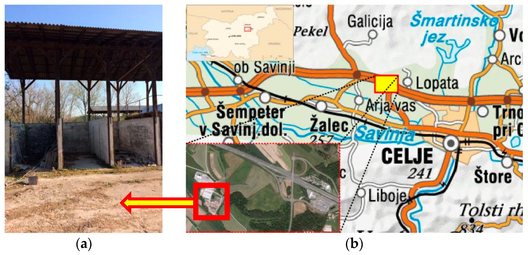
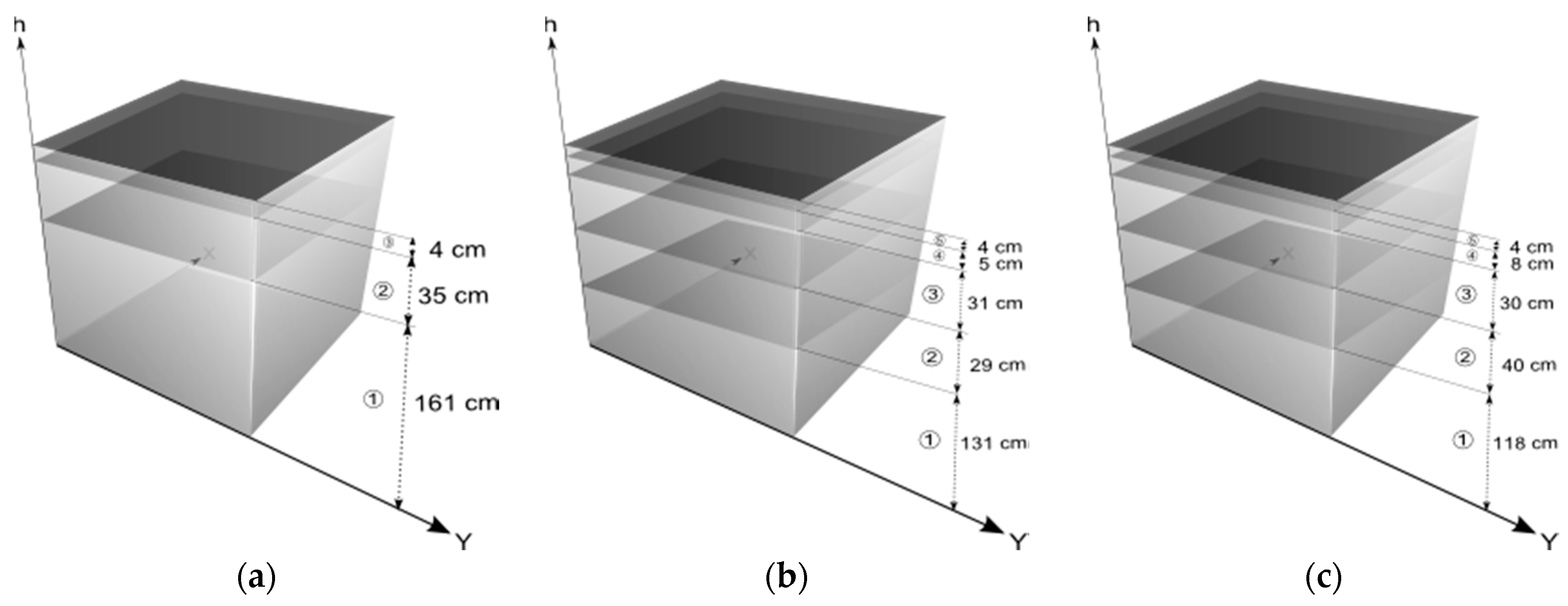
2. Design and Layout of Real Urban Testing Pools: The Establishment of a Geodetic Reference Network and an Estimation of the Positional and Height Accuracy of the Measured UUI
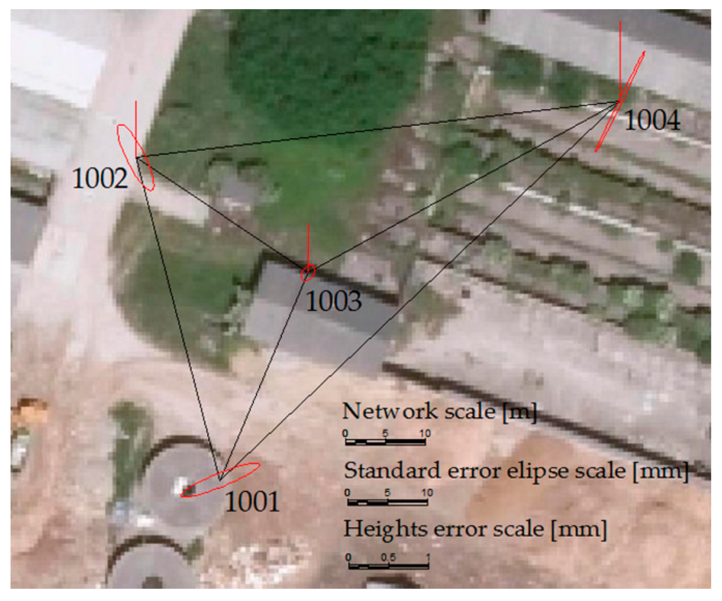
The Establishment of a Geodetic Network for the Purpose of Determining the Position of the UUI and GPR
3. Implementation of the Kinematic GPR-TPS Model
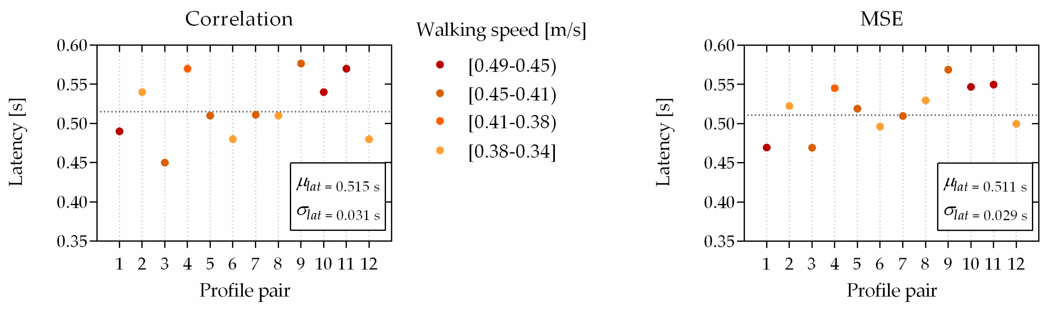
Latency
4. The GPR-TPS Model: Capturing, Processing and Visualising Data
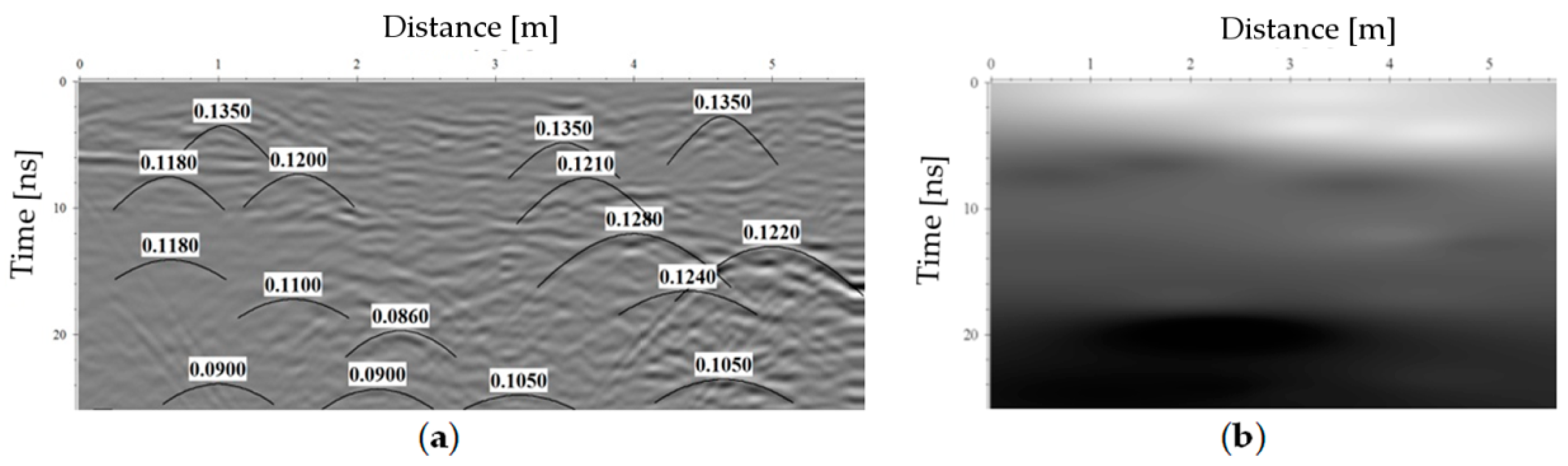
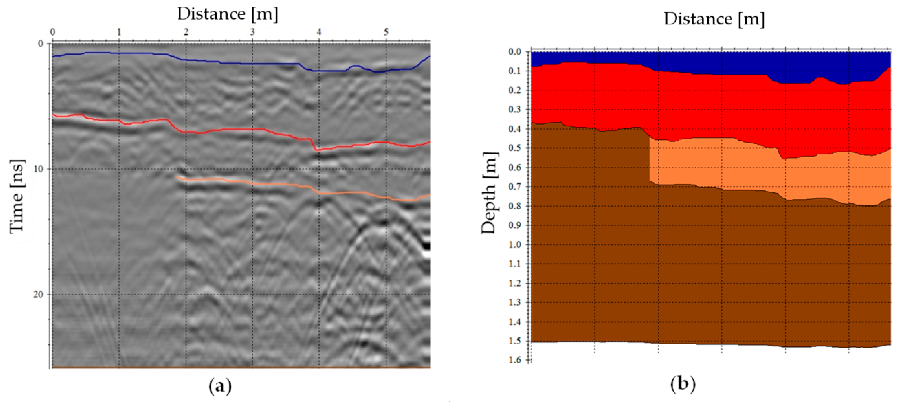
Determining the (Velocity) Depth
5. Results
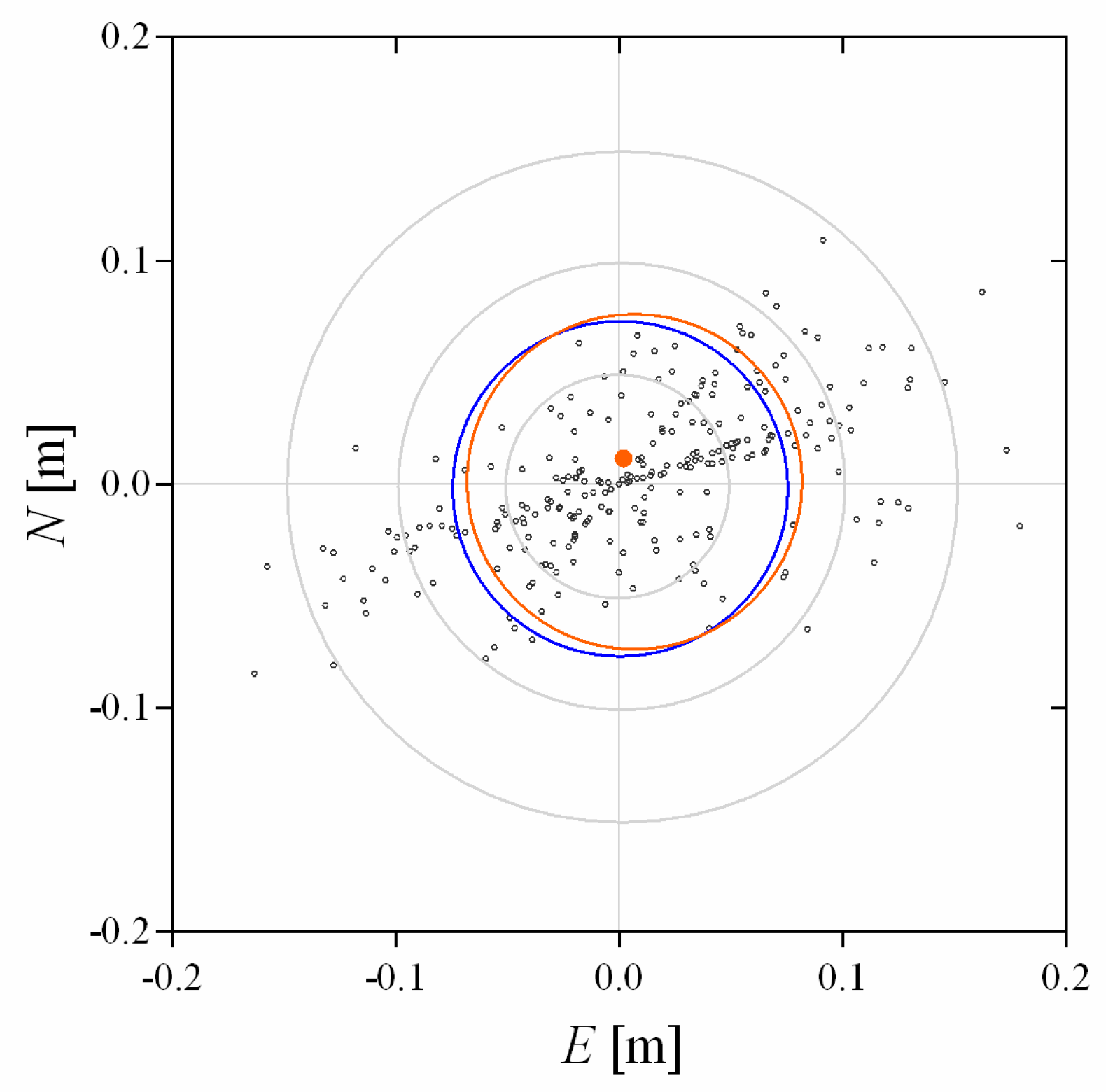
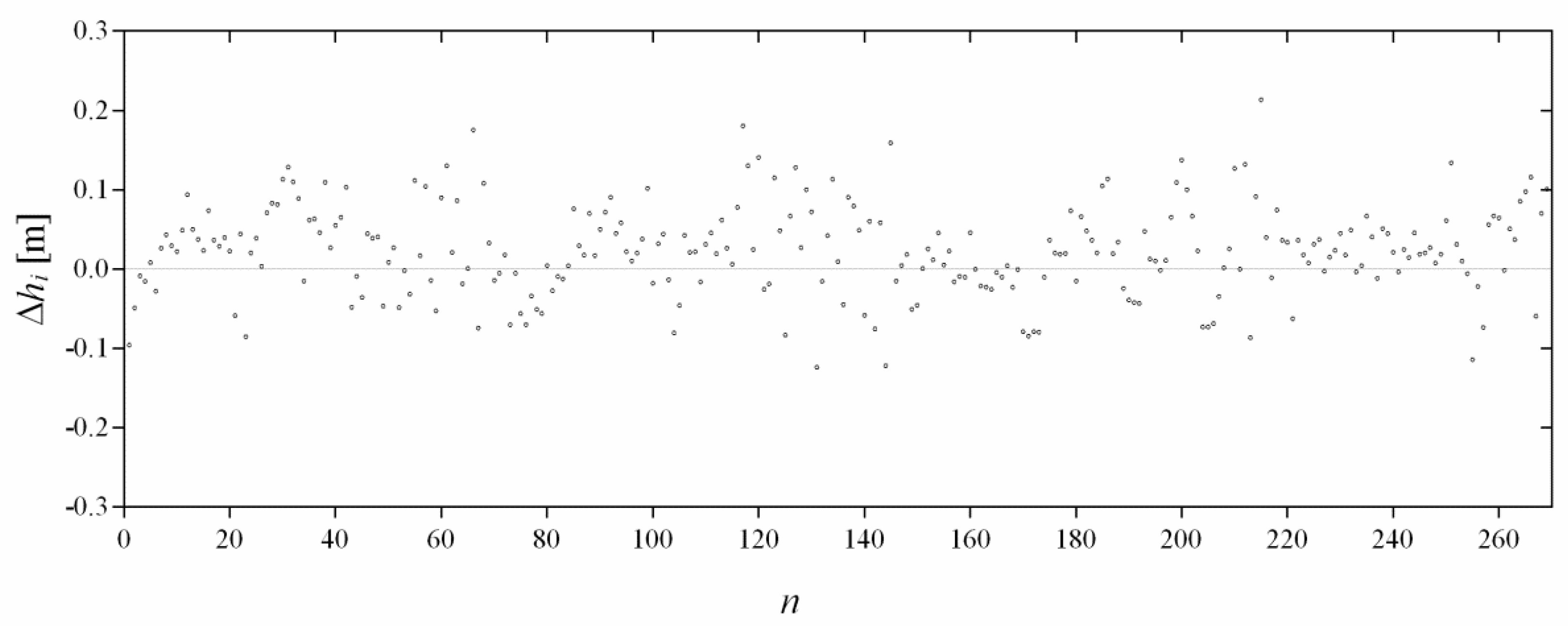
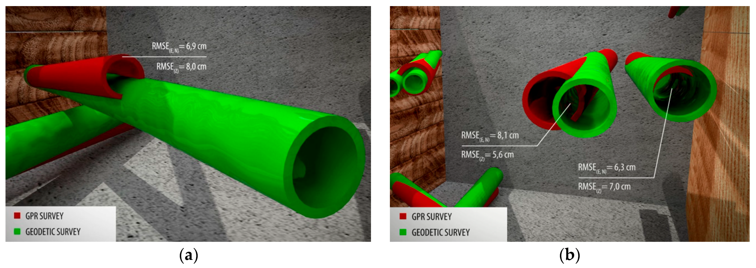
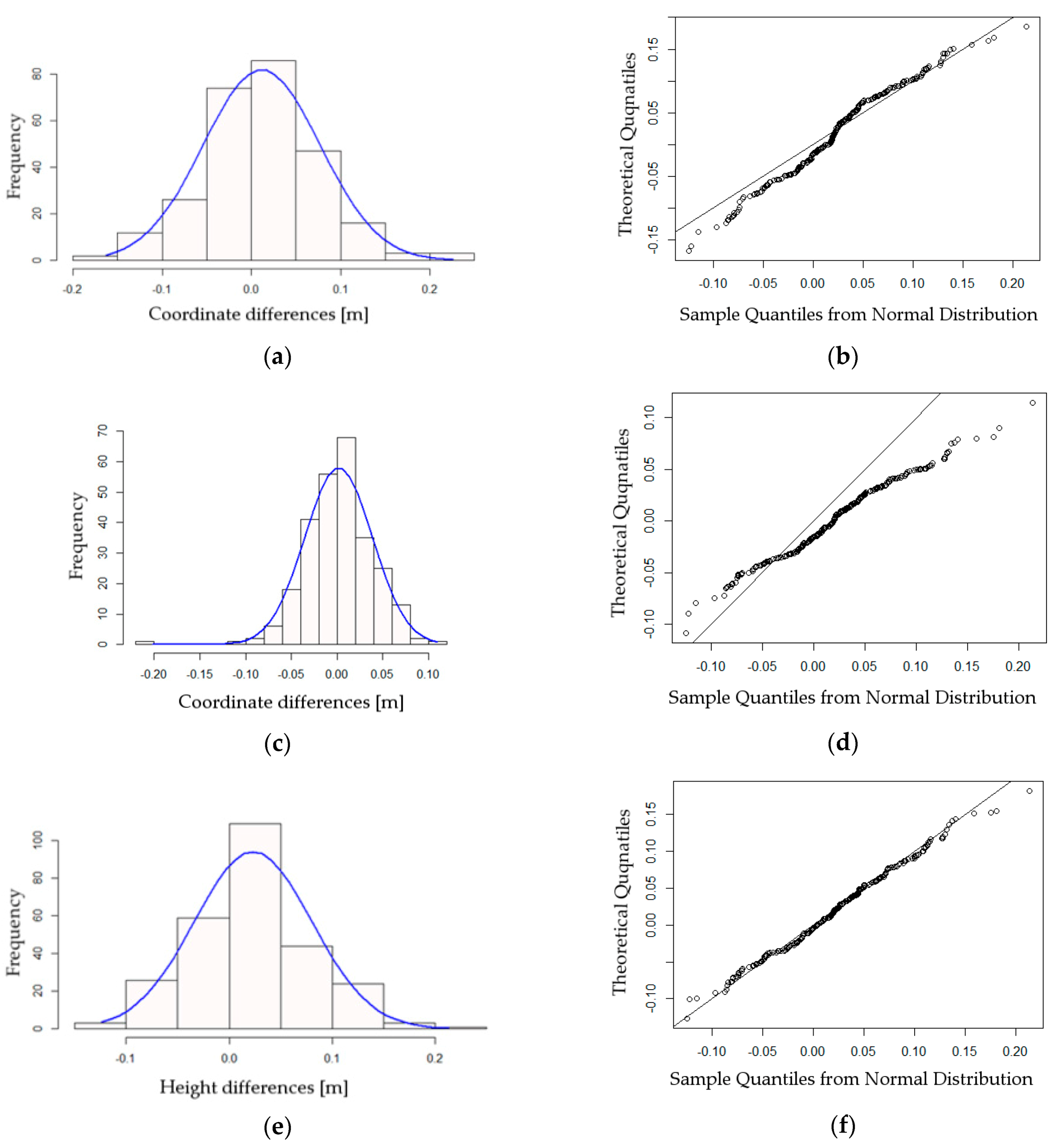
5.1. Accuracy Assessment of the Recorded Position and Height of UUI with the Proposed GPR-TPS Model
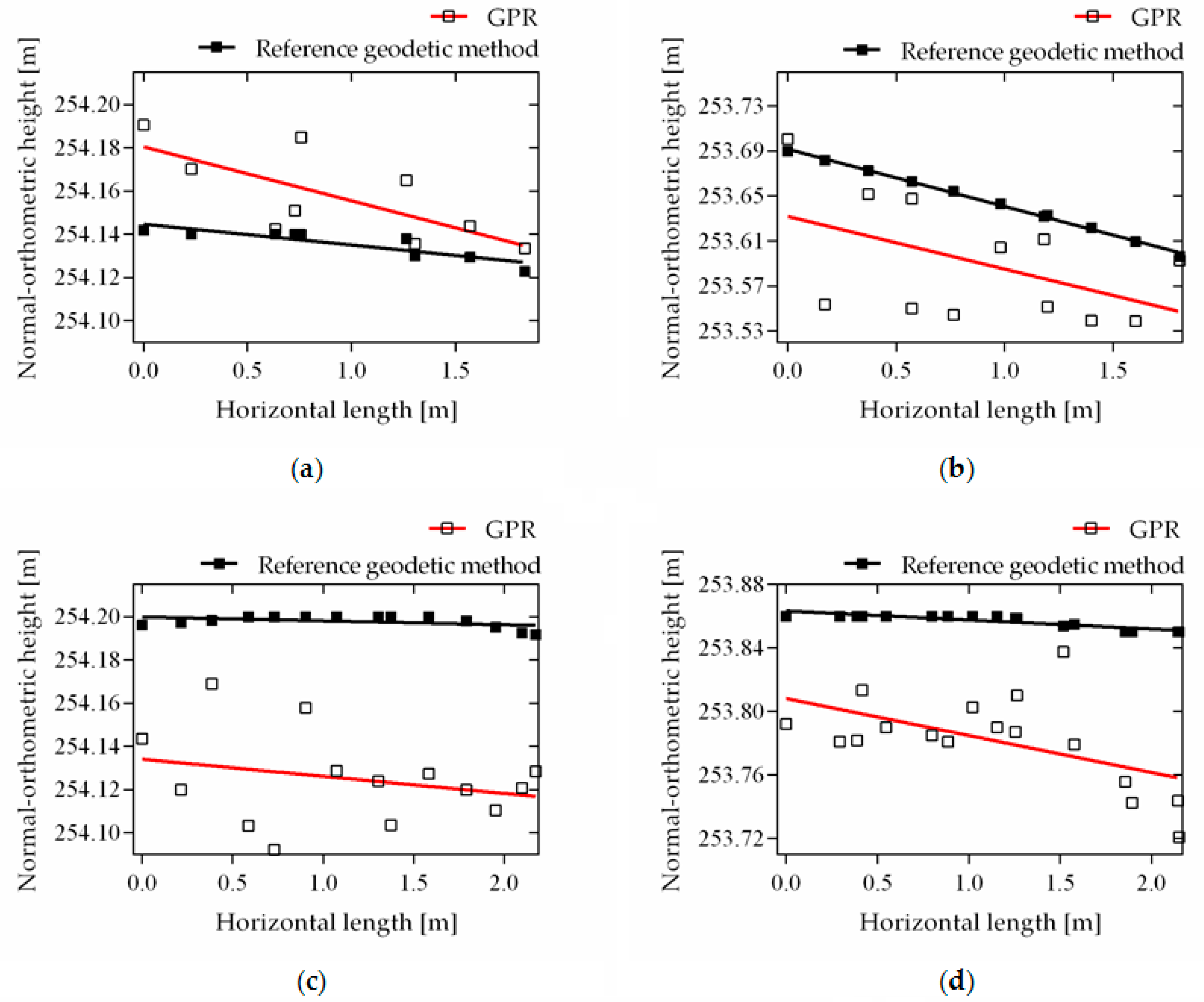
5.2. Assessment of the Incline Accuracy
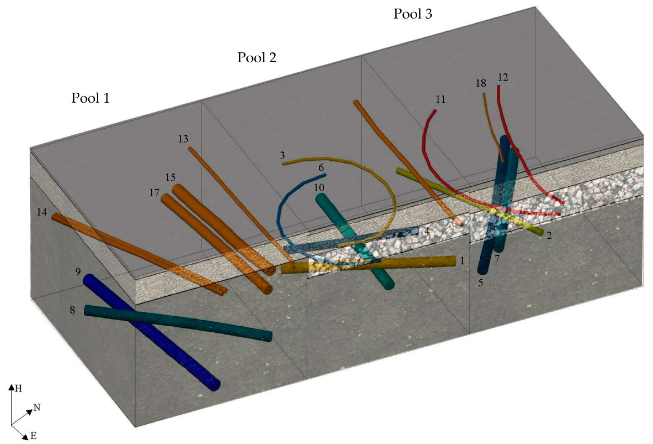
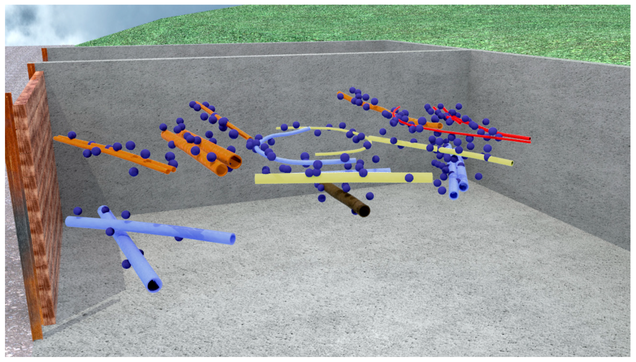
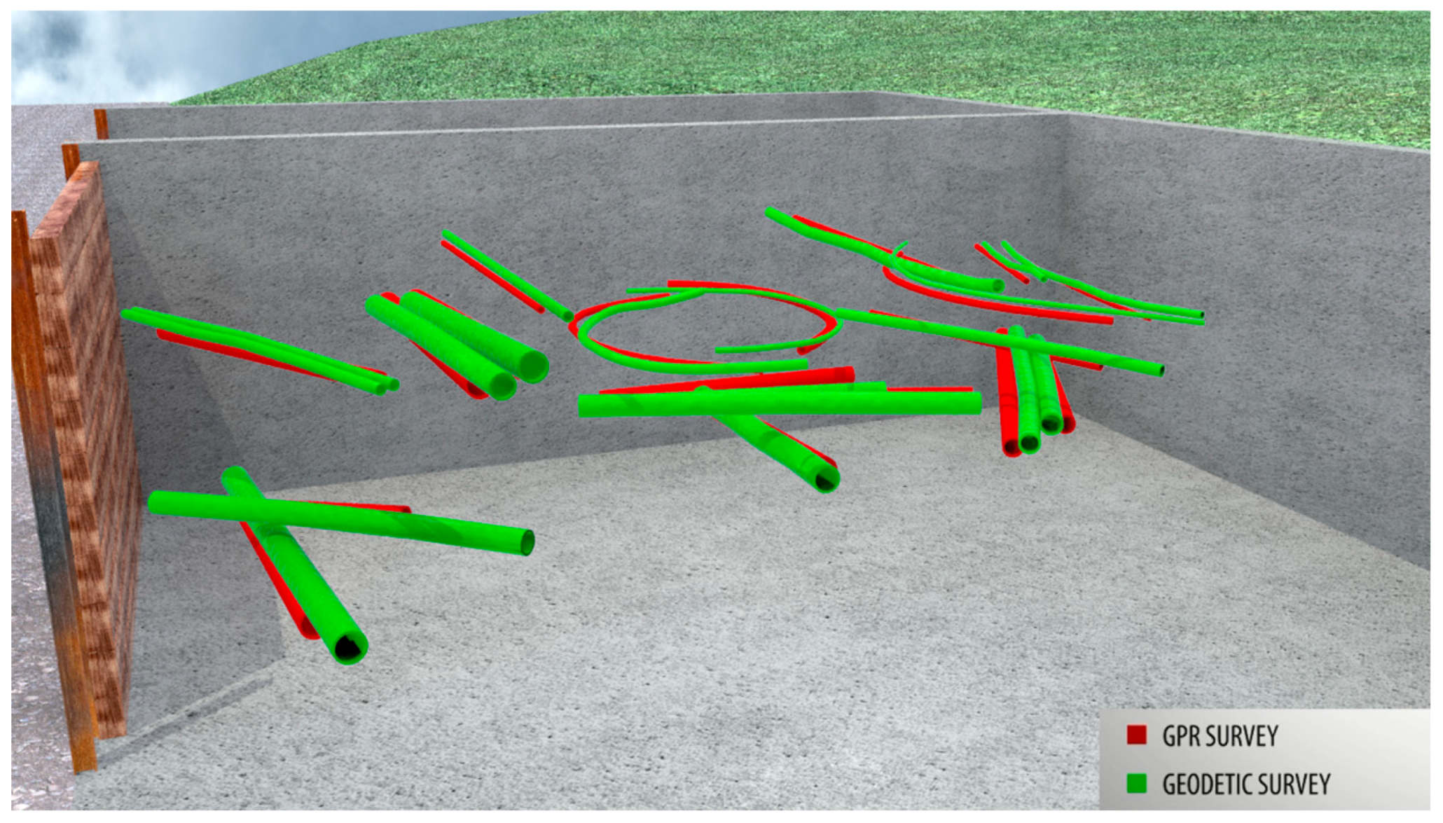
5.3. Graphic Presentation of the Final Results in the Real Urban Testing Pools (3D)
6. Conclusions
Supplementary Materials
Author Contributions
Funding
Acknowledgments
Conflicts of Interest
Appendix A. Adjustment
Appendix B. Normality Tests

References
- Wai-Lok Lai, W.; Dérobert, X.; Annan, P. A review of Ground Penetrating Radar application in civil engineering: A 30-year journey from Locating and Testing to Imaging and Diagnosis. NDT E Int. 2018, 96, 58–78. [Google Scholar] [CrossRef]
- American Society of Civil Engineers. ASCE CI/ASCE38-02. Standard Guideline for the Collection and Depiction of Existing Subsurface Utility Data. ASCE 2002, 38, 1–20. [Google Scholar]
- Annan, P.A. Ground Penetrating Radar, Principles, Procedures and Applications; Sensors & Software Inc.: Mississauga, ON, Canada, 2003. [Google Scholar]
- Barzaghi, R.; Cazzaniga, N.; Pagliari, D.; Pinto, L. Vision-Based Georeferencing of GPR in Urban Areas. Sensors 2016, 16, 132. [Google Scholar] [CrossRef] [PubMed]
- Hao, T.; Rogers, C.D.F.; Metje, N.; Chapman, D.N.; Muggleton, J.M.; Foo, K.Y.; Wang, P.; Pennock, S.R.; Atkins, P.R.; Swingler, S.G.; et al. Condition assessment of the buried utility service infrastructure. Tunn. Undergr. Space Technol. 2012, 28, 331–344. [Google Scholar] [CrossRef]
- Thomas, A.M.; Rogers, C.D.F.; Chapman, D.N.; Metje, N.; Castle, J. Stakeholder needs for ground penetrating radar utility location. J. Appl. Geophys. 2009, 67, 345–351. [Google Scholar] [CrossRef]
- Su, X.; Talmaki, S.; Cai, H.; Kamat, V.R. Uncertainty-aware visualization and proximity monitoring in urban excavation: A geospatial augmented reality approach. Vis. Eng. 2013, 1, 1–13. [Google Scholar] [CrossRef]
- Marvin, S.; Slater, S. Urban infrastructure: The contemporary conflict between roads and utilities. Prog. Plan. 1997, 48, 247–318. [Google Scholar] [CrossRef]
- Talmaki, S.; Kamat, V.R.; Cai, H. Geometric modeling of geospatial data for visualization-assisted excavation. Adv. Eng. Inform. 2013, 27, 283–298. [Google Scholar] [CrossRef]
- Spurgin, J.T.; Lopez, J.; Kerr, K. Utility Damage Prevention—What Can Your Agency Do? American Public Works Association, Congress Session: Kansas City, MO, USA, September 2009; pp. 64–69. [Google Scholar]
- Common Ground Alliance (CGA). 2016 Damage Information Report Tool (DIRT) Report: Analysis and Recommendations; Common Ground Alliance: Arlington, VA, USA, 2017; pp. 1–29. Available online: http://commongroundalliance.com/sites/default/files/publications/DIRT%202016%20Annual%20Report_081017_FINAL_Updated_09.20.17.pdf (accessed on 10 April 2018).
- Osman, H.; El-Diraby, T.E. Evaluating the use of Subsurface Utility Engineering in Canada. Transportation Research Board, 86th Annual Meeting. 2007, pp. 1–18. Available online: http://docs.trb.org/prp/07-0307.pdf (accessed on 11 May 2018).
- AS 5488—2013. Australian Standard: Classification of Subsurface Utility Information. 2013. Available online: https://nulca.com.au/db_uploads/5488-2013_V2.pdf (accessed on 21 April 2018).
- ICE PAS 128: 2014. British Standard: Specification for Underground Utility Detection, Verification and Location Institute of Civil Engineer; British Standards Institution: London, UK, 2014. [Google Scholar]
- Šarlah, N. Development of the Georadar Observation Model for Underground Infrastructure Detection. Ph.D. Dissertation, University of Ljubljana, Faculty of Civil and Geodetic Engineering, Ljubljana, Slovenia, 2016. Available online: https://repozitorij.uni-lj.si/Dokument.php?id=97913&lang=slv (accessed on 27 April 2018).
- Rakar, A.; Šubic-Kovač, M.; Mesner, A.; Mlinar, J.; Šarlah, N. Zaščita in ohranjanje vrednosti gospodarske javne infrastrukture. Geod. Vestn. 2010, 54, 242–252. [Google Scholar] [CrossRef]
- Gurbuz, A.C. Feature Detection Algorithms in Computed Images. Ph.D. Dissertation, Institute of Technology Georgia, Atlanta, GA, USA, 2008. [Google Scholar]
- Singh, N.P.; Nene, M.J. Buried object detection and analysis of GPR images: Using neural network and curve fitting. In Proceedings of the Annual International Conference on Emerging Research Areas and International Conference on Microelectronics, Communications and Renewable Energy, Kanjirapally, India, 4–6 June 2013. [Google Scholar]
- Li, S.; Cai, H.; Kamat, V.R. Uncertainty-aware geospatial system for mapping and visualizing underground utilities. Autom. Constr. 2015, 53, 105–119. [Google Scholar] [CrossRef]
- Ayala-Cabrera, D.; Herrera, M.; Izquierdo, J.; Ocaña–Levario, S.J.; Pérez-García, R. GPR-Based Water Leak Models in Water Distribution Systems. Sensors 2013, 13, 15912–15936. [Google Scholar] [CrossRef]
- Cheng, N.-F.; Tang, H.-W.; Chan, C.-T. Identification and positioning of underground utilities using ground penetrating radar (GPR). Sustain. Environ. Res. 2013, 23, 141–152. [Google Scholar]
- Metwaly, M. Application of GPR technique for subsurface utility mapping: A case study from urban area of Holy Mecca. Saudi Arabia. Measurement 2015, 60, 139–145. [Google Scholar] [CrossRef]
- Millington, T.M.; Cassidy, N.J. Optimising GPR modelling: A practical, multi-threaded approach to 3D FDTD numerical modelling. Comput. Geosci. 2009, 36, 1135–1144. [Google Scholar] [CrossRef]
- Sagnard, F.; Norgeot, C.; Derobert, X.; Baltazart, V.; Merliot, E.; Derkx, F.; Lebental, B. Utility detection and positioning on the urban site Sense-City using Ground-Penetrating Radar systems. Measurement 2016, 88, 318–330. [Google Scholar] [CrossRef] [Green Version]
- Jeng, Y.; Chen, C.-S. Subsurface GPR imaging of a potential collapse area in urban environments. Eng. Geol. 2012, 147–148, 57–67. [Google Scholar] [CrossRef]
- Lehmann, F.; Green, A.G. Semiautomated georadar data acquisition in three dimensions. Geophysics 1999, 64, 719–731. [Google Scholar] [CrossRef]
- Böniger, U.; Tronicke, J. On the Potential of Kinematic GPR Surveying Using a Self-Tracking Total Station: Evaluating System Crosstalk and Latency. IEEE Trans. Geosci. Remote Sens. 2010, 48, 3792–3798. [Google Scholar] [CrossRef]
- Aaltonen, J.; Nissen, J. Geological mapping using GPR and differential GPS positioning: A case. In Proceedings of the Ninth International Conference on Ground Penetrating Radar, Santa Barbara, CA, USA, 29 April–2 May 2002. [Google Scholar]
- Young, R.A.; Lord, N. A hybrid laser-tracking/GPS location method allowing GPR acquisition in rugged terrain. Lead. Edge 2002, 21, 486–490. [Google Scholar] [CrossRef]
- Grasmueck, M.; Viggiano, D.A. Integration of Ground-Penetrating Radar and Laser Position Sensors for Real-Time 3-D Data Fusion. IEEE Trans. Geosci. Remote Sens. 2007, 45, 130–137. [Google Scholar] [CrossRef]
- Dimc, F.; Music, B.; Osredkar, R. Attaining Required Positioning Accuracy in Archeo-Geophysical Surveying by GPS. In Proceedings of the 12th International Power Electronics and Motion Control Conference, Portorož, Slovenia, 30 August–1 September 2006. [Google Scholar]
- Mohsen, J.P.; Rockaway, T.D.; Gupta, D.K. Test Field Design and development for GPR Techniques for Infrastructure Asset Identification. In Proceedings of the 11th International Conference on Ground Penetrating Radar, Columbus, OH, USA, 19–22 June 2006. [Google Scholar]
- Grandjean, G.; Gourry, J.C.; Bitri, A. Evaluation of GPR techniques for civil-engineering applications: Study on a test site. J. Appl. Geophys. 2000, 45, 141–156. [Google Scholar] [CrossRef]
- Shahbaz-Khan, U. Interpretation of Ground Penetrating Radar Data for Utilities—Methods Techniques and Implementation; VDMVerlang Dr. Muller GmbH & Co.: Saarbrucken, Germany, 2011; pp. 1–200. [Google Scholar]
- TSC 06.300/06.410:2009. Smernice in tehnični pogoji za graditev asfaltnih plasti; Direkcija Republike Slovenije za ceste: Ljubljana, Slovenia, 2009; pp. 8–28.
- TSC 06.511:2009. Tehnična specifikacija za prometno obremenitev—določitev in razvrstitev; Direkcija Republike Slovenije za ceste: Ljubljana, Slovenia, 2009; pp. 1–10.
- TSC 06.512:2003. Tehnična specifikacija za projektiranje—klimatski in hidrološki pogoji; Direkcija Republike Slovenije za ceste: Ljubljana, Slovenia, 2003; pp. 4–11.
- TSC 06.520:2009. Tehnična specifikacija za projektiranje—dimenzioniranje novih asfaltnih voziščnih konstrukcij; Direkcija Republike Slovenije za ceste: Ljubljana, Slovenia, 2009; pp. 8–22.
- Medved, K.; Bajec, K.; Berk, S.; Koler, B.; Kuhar, M.; Radovan, D.; Sterle, O.; Stopar, B. National Report of Slovenia to the EUREF 2010 Symposium in Gävle. Report on the Symposium of the IAG Sub—Commission for Europe (EUREF), Gävle, Sweden, 2–5 June 2010. Available online: http://www.euref.eu/symposia/2010Gavle/07-26-p-Slovenia.pdf (accessed on 11 May 2018).
- Martín, A.; Padín, J.; Anquela, A.B.; Sánchez, J.; Belda, S. Compact Integration of a GSM-19 Magnetic Sensor with High-Precision Positioning using VRS GNSS Technology. Sensors 2009, 9, 2944–2950. [Google Scholar] [CrossRef] [PubMed] [Green Version]
- Šarlah, N.; Štebe, G.; Sterle, O. Postopek vzpostavitve in testiranja lastne referenčne GNSS-postaje. Geod. Vestn. 2015, 59, 457–472. [Google Scholar] [CrossRef]
- Uren, L.; Price, W.F. Surveying for Engineers, 4th ed.; Palgrave Macmillan: New York, NY, USA, 2006; pp. 1–824. [Google Scholar]
- Kirschner, H.; Stempfhuber, W. The Kinematic Potential of Modern Tracking Total Stations—A State of the Art Report on the Leica TPS1200+. In Proceedings of the 1st International Conference on Machine Control & Guidance, Kinematic Measurement and Sensor Technology I (Local Systems), Zurich, Switzerland, 24–26 June 2008; pp. 1–10. [Google Scholar]
- Leica TPS1200+; User Manual; Leica Geosystems: Heerbrugg, Switzerland, 2008; pp. 1–209. Available online: http://www.surveyequipment.com/PDFs/TPS1200_User_Manual.pdf (accessed on 14 April 2018).
- Sandmeier, K.J. ReflexW Manual, Version 7.5 Windows™9x/NT/XP/7 Program for the Processing and Interpretation of Reflection and Transmission Data. 2014, pp. 1–598. Available online: http://www.sandmeier-geo.de/download.html (accessed on 23 March 2018).
- Zitová, B.; Flusser, J. Image registration methods: A survey. Image Vis. Comput. 2003, 21, 977–1000. [Google Scholar] [CrossRef]
- Fonseca, L.M.G.; Manjunath, B.S. Registration techniques for multisensor remotely sensed imagery. Photogramm. Eng. Remote Sens. 1996, 62, 1049–1056. [Google Scholar]
- Wang, Z.; Bovik, A.C. Mean squared error: Love it or leave it? A new look at Signal Fidelity Measures. IEEE Signal Process. Mag. 2009, 26, 98–117. [Google Scholar] [CrossRef]
- Gonzales, R.C.; Woods, R.E. Digital Image Processing; Pearson Prentice Hall: Upper Saddle River, NJ, USA, 2008. [Google Scholar]
- Wang, Z.; Bovik, A.C. A universal image quality index. IEEE Signal Process. Lett. 2002, 9, 81–84. [Google Scholar] [CrossRef]
- Kumar, R.; Rattan, M. Analysis of Various Quality Metrics for Medical Image Processing. Int. J. Adv. Res. Comput. Sci. Softw. Eng. 2012, 2, 137–144. [Google Scholar]
- Yilmaz, Ö.; Doherty, S.M. Seismic Data Processing; Investigations in Geophysics 2; Society of Exploration Geophysicists: Tulsa, OK, USA, 1987; pp. 1–526. [Google Scholar]
- Conyers, L.B. Ground-Penetrating Radar for Archaeology, 3rd ed.; Altamira Press: Lanham, MD, USA, 2013. [Google Scholar]
- Tillard, S. Analysis of GPR data: Wave propagation velocity determination. J. Appl. Geophys. 1995, 33, 77–91. [Google Scholar] [CrossRef]
- Leckebusch, J. Two and Three-Dimensional Ground Penetrating Radar Surveys across a Medieval Choir: A Case Study in Archaeology. Archaeol. Prospect. 2000, 7, 189–200. [Google Scholar] [CrossRef]
- Höhle, J.; Höhle, M. Accuracy assessment of digital elevation models by means of robust statistical methods. ISPRS J. Photogramm. Remote Sens. 2009, 64, 398–406. [Google Scholar] [CrossRef] [Green Version]
- Kohlrausch, F. Praktische Physik, Band 2, 23rd ed.; Teubner: Stuttgart, Germany, 1985. [Google Scholar]
- Thoode, H.C. Testing for Normality; Marcel Dekker: New York, NY, USA, 2002; pp. 1–479. [Google Scholar]
- Stephens, M.A. EDF Statistics for Goodness of Fit and Some Comparisons. J. Am. Stat. Assoc. 1974, 69, 730–737. [Google Scholar] [CrossRef]
- Anderson, T.W.; Darling, D.A. A Test of Goodness-of-Fit. J. Am. Stat. Assoc. 1954, 49, 765–769. [Google Scholar] [CrossRef]
- D’Agostino, R.B.; Stephens, M.A. Goodness of Fit Technique; Marcel Dekker: New York, NY, USA, 1986. [Google Scholar]
- Ghasemi, A.; Zahediasl, S. Normality Tests for Statistical Analysis: A Guide for Non-Statisticians. Int. J. Endocrinol. Metab. 2012, 10, 486–489. [Google Scholar] [CrossRef] [PubMed] [Green Version]


| Object No. | Type | Manufacturer | Material | Nominal Diameter ND/OD [mm] | Depth [cm] | Pool No. |
|---|---|---|---|---|---|---|
| 1 | Gas | Drinplast | PE 100 | 100 | 120 | 2 |
| 2 | Gas | KontiHidroplast | PE 100 | 63 | 110 | 3 |
| 3 | Gas | TotraPlastika | PE 100 | 32 | 80 | 2 |
| 4 | Water | TotraPlastika | PE 80 | 90 | 130 | 2 |
| 5 | Water | TotraPlastika | PE 80 | 110 | 150 | 3 |
| 6 | Water | Deriplast | PE 80 | 32 | 80 | 2 |
| 7 | Water | Tubi PVC | PVC | 110 | 150 | 3 |
| 8 | Water | Tubi PVC | PVC | 110 | 160 | 1 |
| 9 | Water | SvoodnySokol | Duktil | 110 | 180 | 1 |
| 10 | Sewage | OsterndorfKun. | PE 200 | 125 | 170 | 1 |
| 11 | Electrical | Elka | Al/PE HD | 31 | 80 | 3 |
| 12 | Electrical | SKW | Al/PE HD | 31.2 | 80 | 3 |
| 13 | ELC | Minerva | PE 80 | 125 | 80 | 1 |
| 14 | ELC | Rumaplast | PE 80 | 2 × 50 | 80 | 1 |
| 15 | ELC | Miner.- Mapitel | PE 80 | 40 | 40 | 1 |
| 16 | ELC | Miner.- Mapitel | PE 80 | 50 | 40 | 2 |
| 17 | ELC | Minerva | PE 80 | 110 | 80 | 1 |
| 18 | Coax | Commscope | Cu/PE 80 | 24.4 | 80 | 3 |
| Process | Parameters 900 (MHz) | Parameters 400 (MHz) |
| DC shift, interval (ns) | 20–25 | 50–70 |
| Time zero correction (ns) | 3.90 | 5.73 |
| Manual signal gain, gain factor (dB) | 0–36 | 0–33 |
| Band-pass frequency with tapered cosine window (MHz) | 420/630/1370/1700 | 230/320/580/750 |
| f-k filtering limited by reflections for the positive and negative directions (m/ns) | +0.105 to +0.065 −0.055 to −0.085 | +0.098 to +0.057 −0.043 to −0.072 |
| Subtracting average (traces) | 65 | 50 |
| Determination of 2D velocity field, interval (m/ns) | 0.080–0.132 | 0.080–0.131 |
| Kirchhoff 2D time migration, ∑ width (Number of traces) | 20 | 30 |
| Manual signal gain, gain factor (dB) | 0–25 | 0–25 |
| Time to depth conversion, max depth axis (m) | 1.6 | 2.1 |
© 2019 by the authors. Licensee MDPI, Basel, Switzerland. This article is an open access article distributed under the terms and conditions of the Creative Commons Attribution (CC BY) license (http://creativecommons.org/licenses/by/4.0/).
Share and Cite
Šarlah, N.; Podobnikar, T.; Mongus, D.; Ambrožič, T.; Mušič, B. Kinematic GPR-TPS Model for Infrastructure Asset Identification with High 3D Georeference Accuracy Developed in a Real Urban Test Field. Remote Sens. 2019, 11, 1457. https://0-doi-org.brum.beds.ac.uk/10.3390/rs11121457
Šarlah N, Podobnikar T, Mongus D, Ambrožič T, Mušič B. Kinematic GPR-TPS Model for Infrastructure Asset Identification with High 3D Georeference Accuracy Developed in a Real Urban Test Field. Remote Sensing. 2019; 11(12):1457. https://0-doi-org.brum.beds.ac.uk/10.3390/rs11121457
Chicago/Turabian StyleŠarlah, Nikolaj, Tomaž Podobnikar, Domen Mongus, Tomaž Ambrožič, and Branko Mušič. 2019. "Kinematic GPR-TPS Model for Infrastructure Asset Identification with High 3D Georeference Accuracy Developed in a Real Urban Test Field" Remote Sensing 11, no. 12: 1457. https://0-doi-org.brum.beds.ac.uk/10.3390/rs11121457