The Messapic Site of Muro Leccese: New Results from Integrated Geophysical and Archaeological Surveys

 ,
, 
Abstract
:1. Introduction
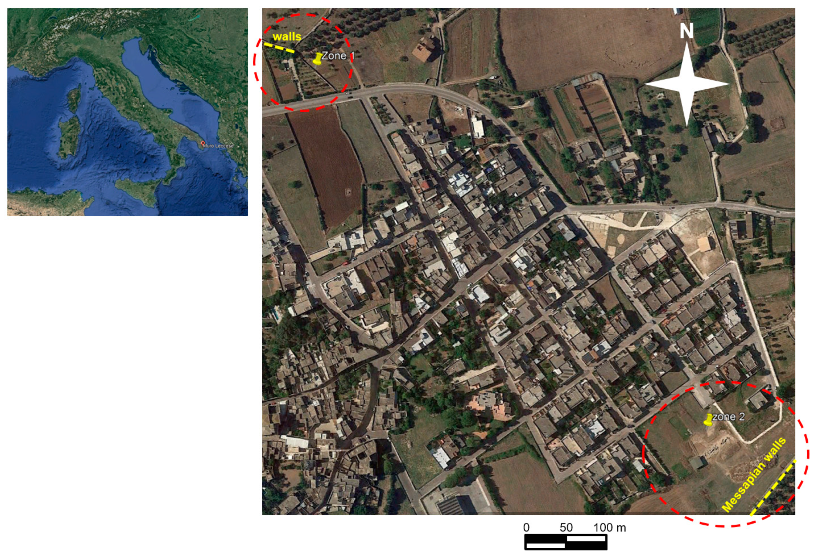
2. Site Description
3. Materials and Methods
3.1. Zone 1
3.2. Zone 2
4. Results
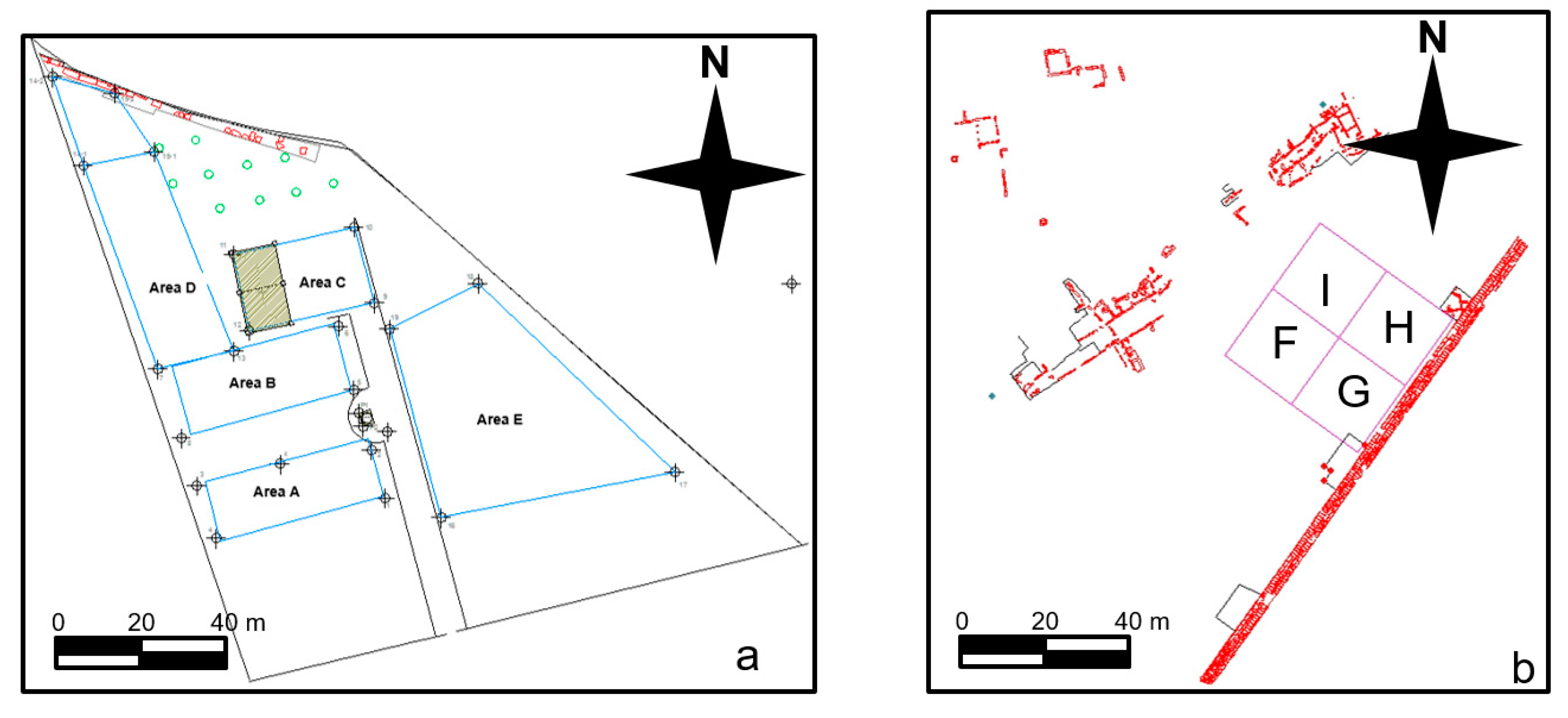
4.1. ZONE 1
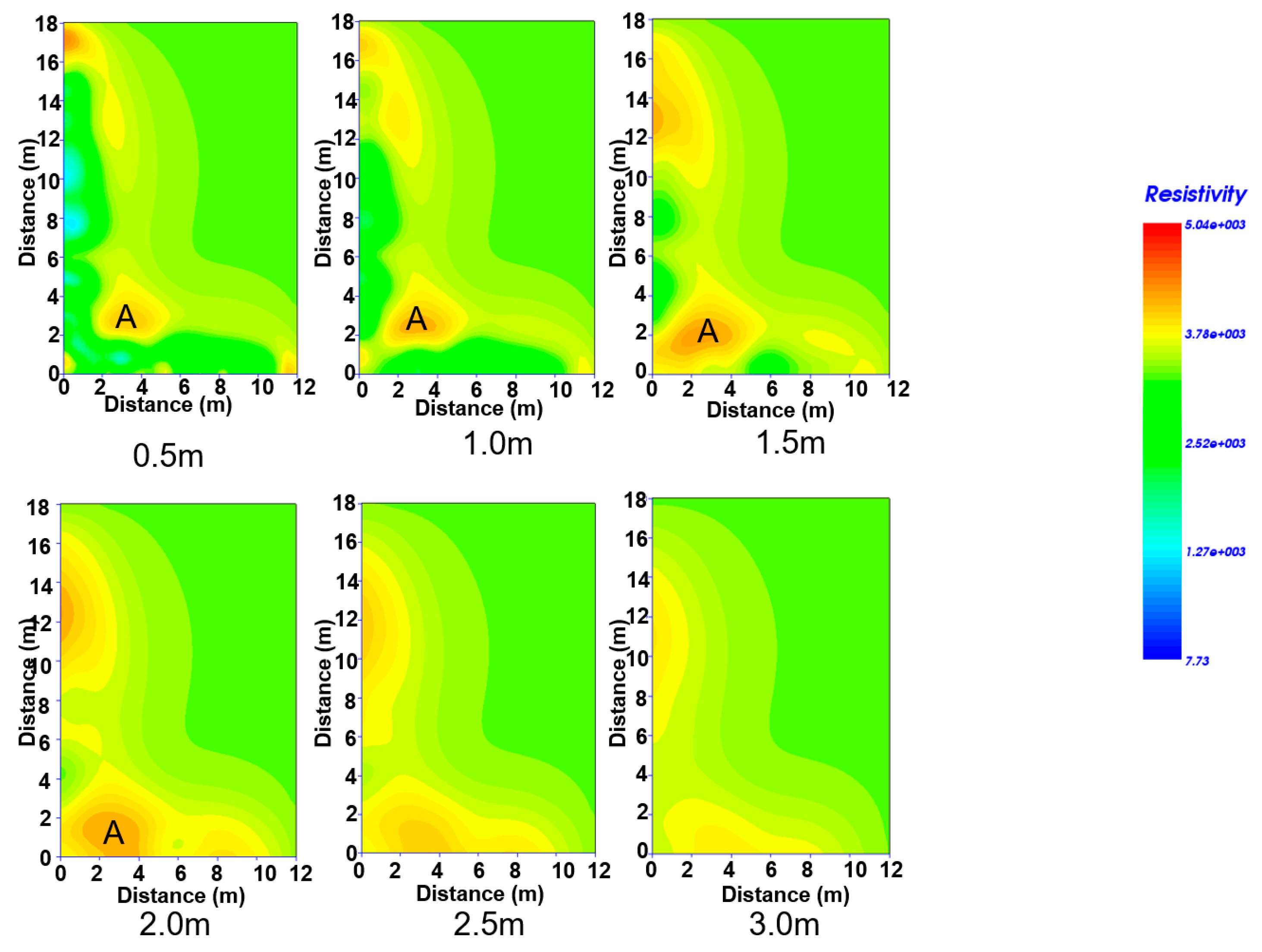
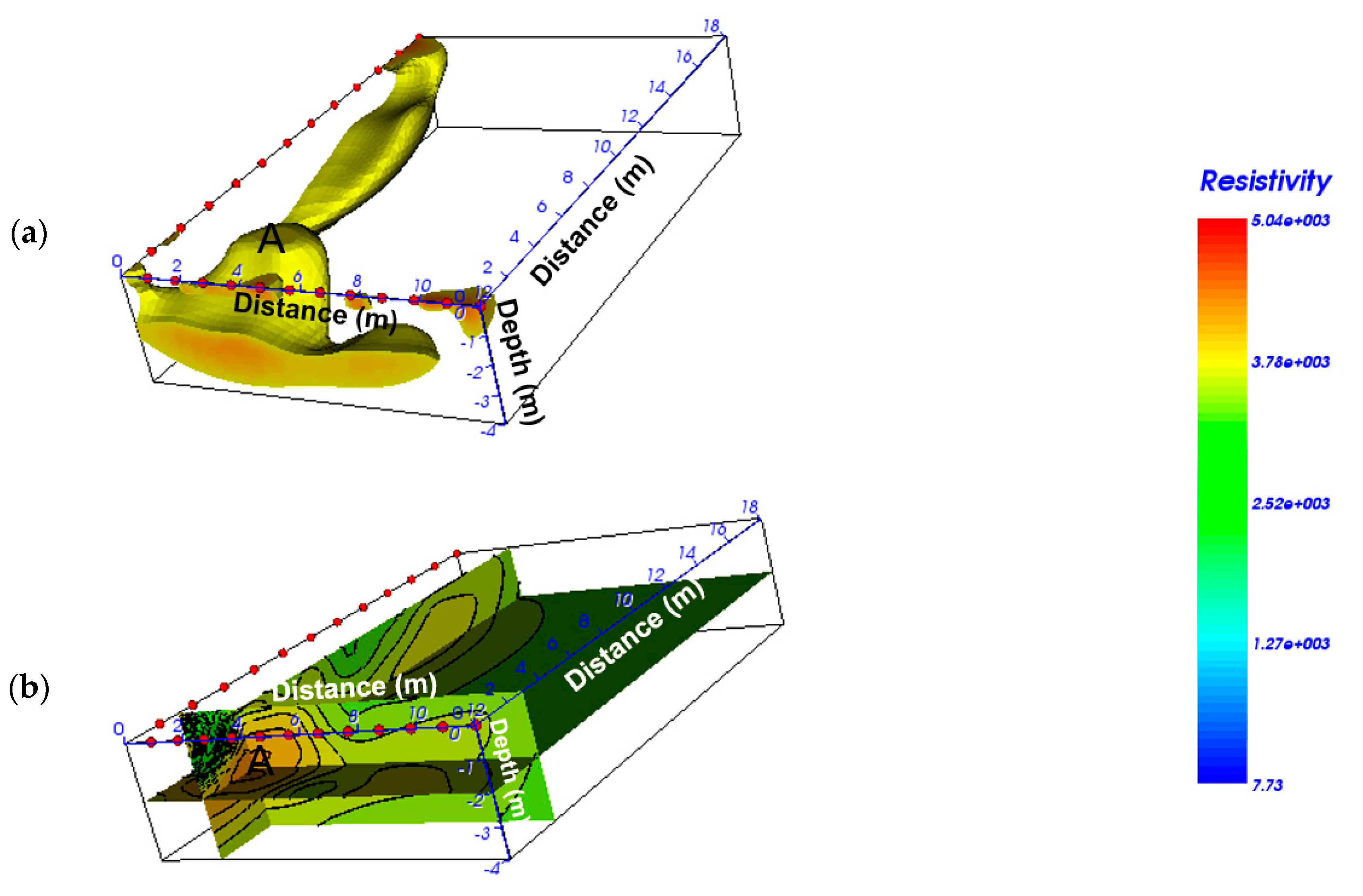
4.1.1. Zone 1, Area A
4.1.2. Zone 1, Area B
4.1.3. Zone 1, Area C
4.1.4. Zone 1, Area D
4.1.5. Zone 1, Area E
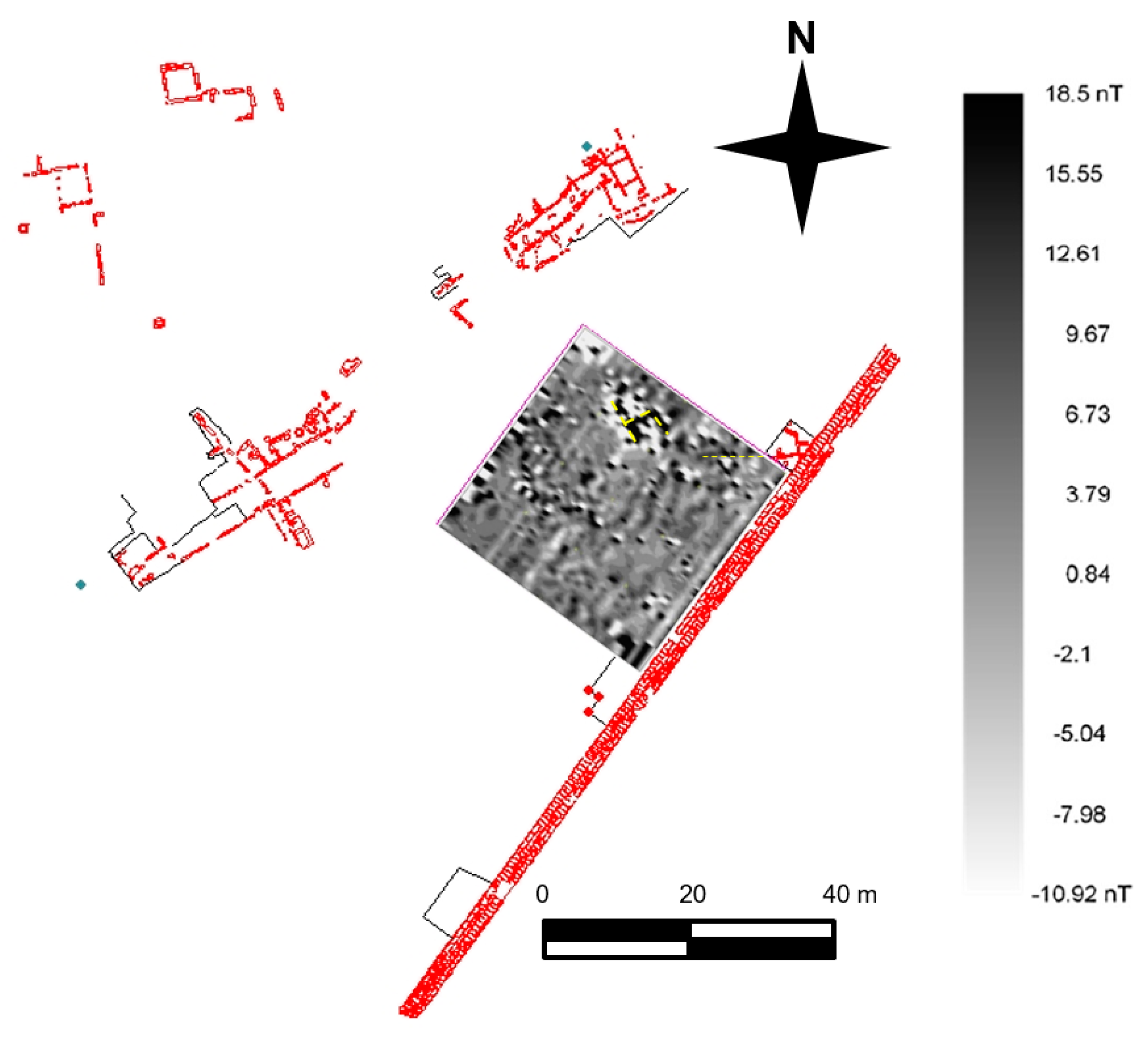
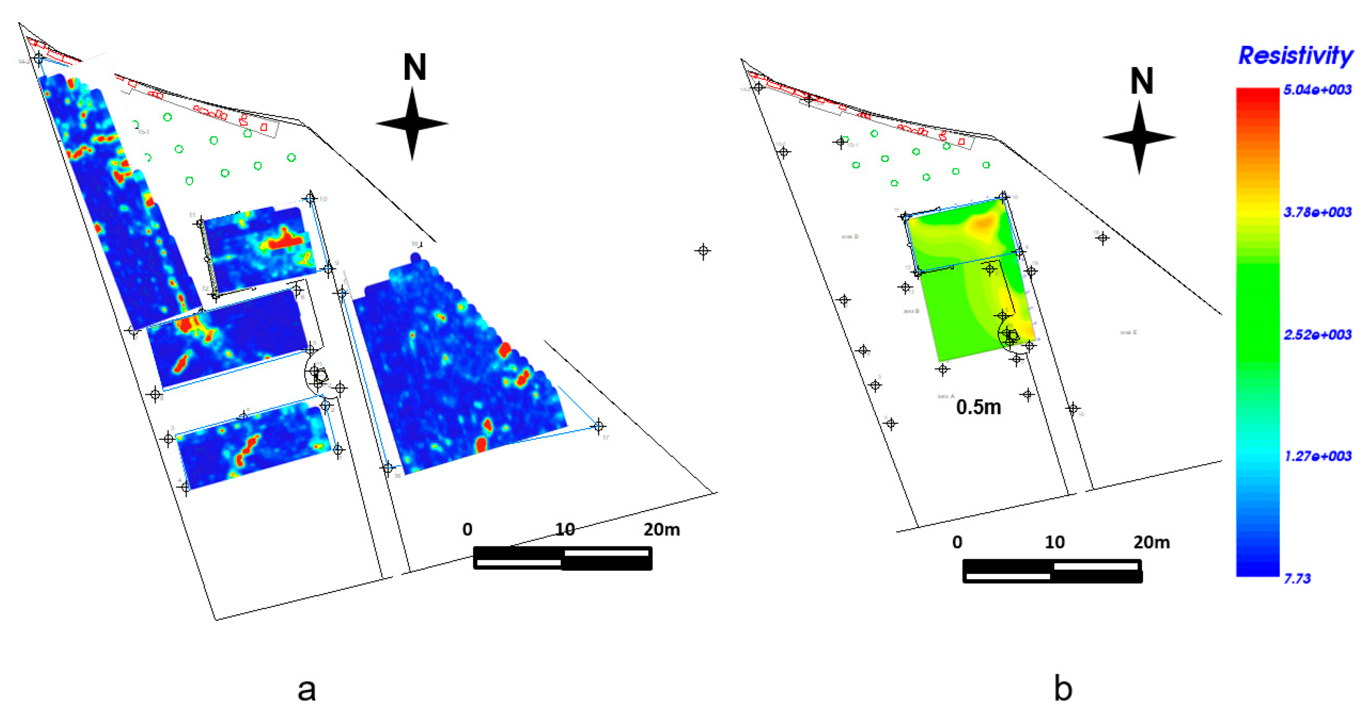
4.2. Zone 2
4.2.1. Zone 2: Magnetic Data Analysis
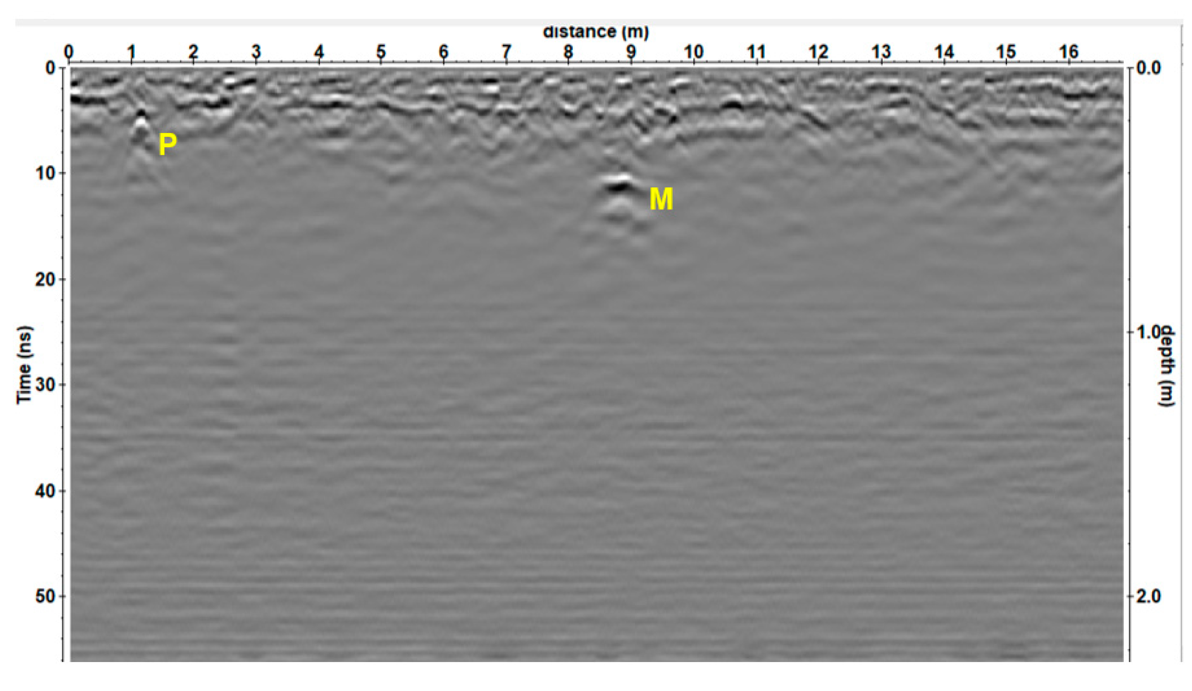
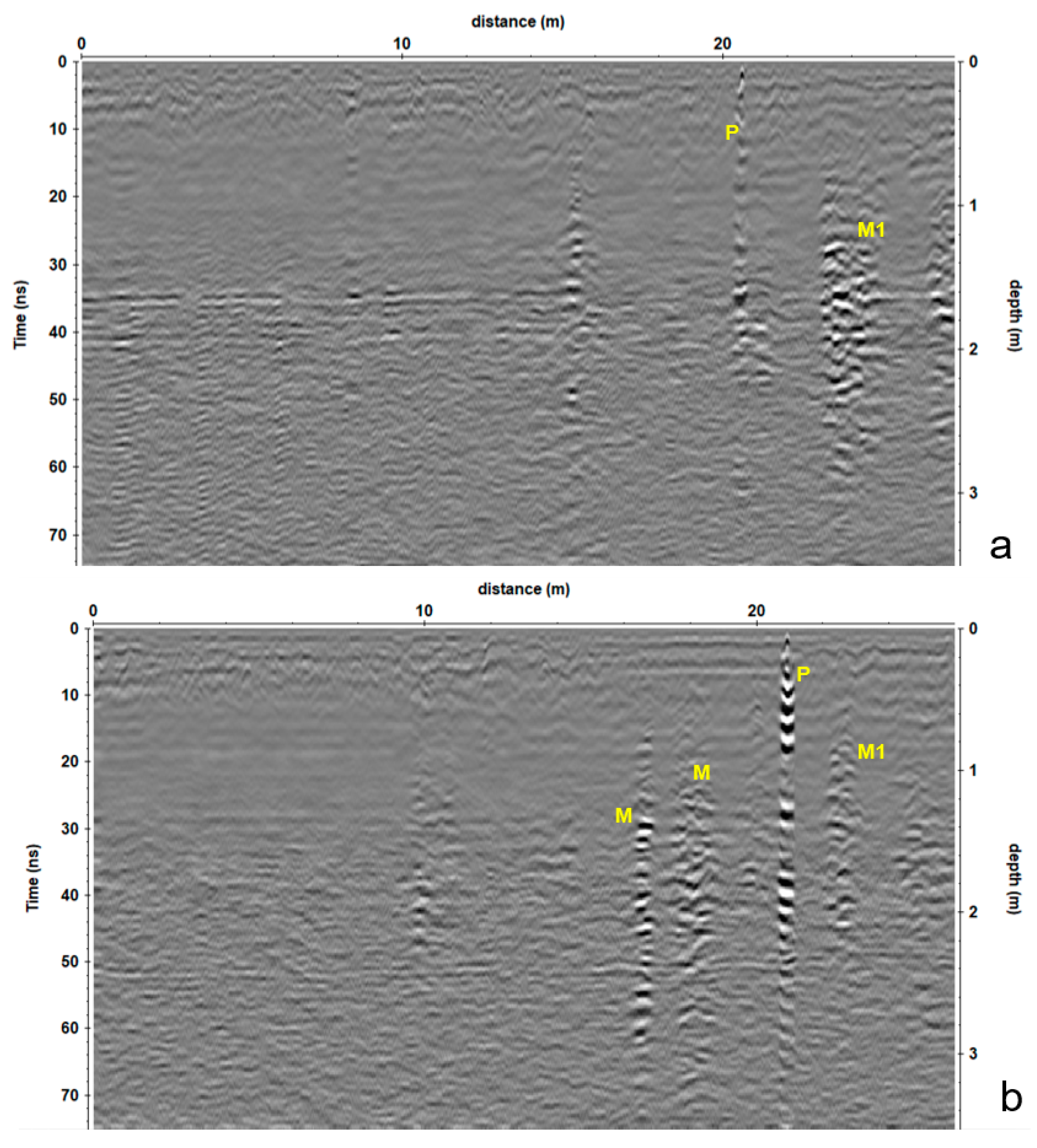
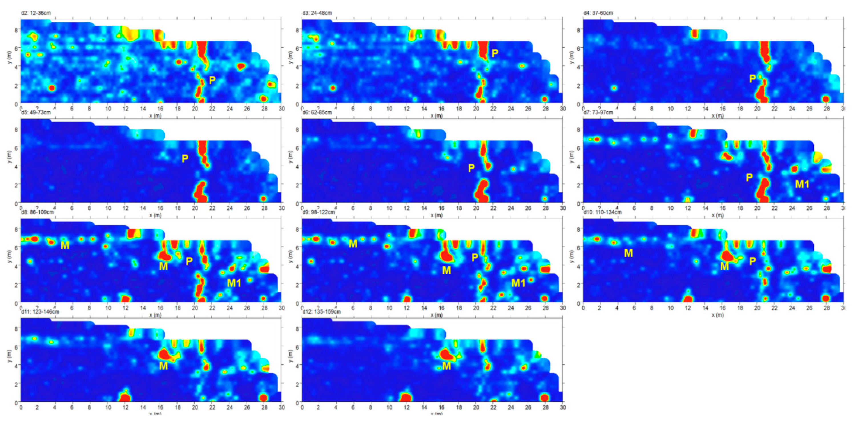
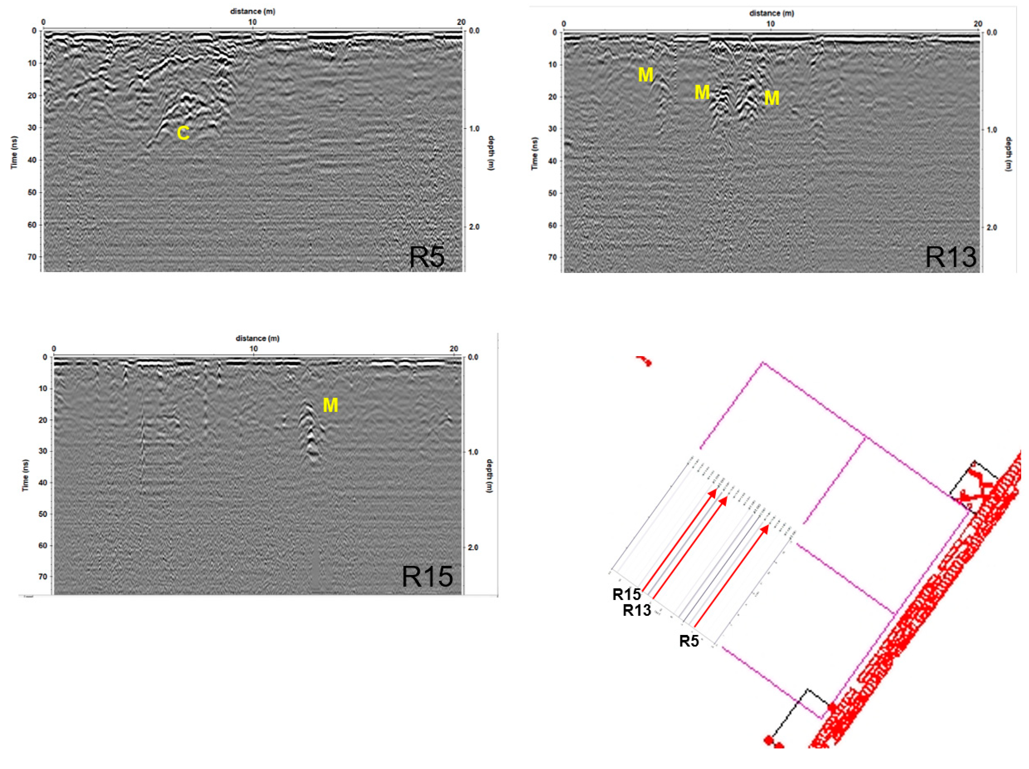
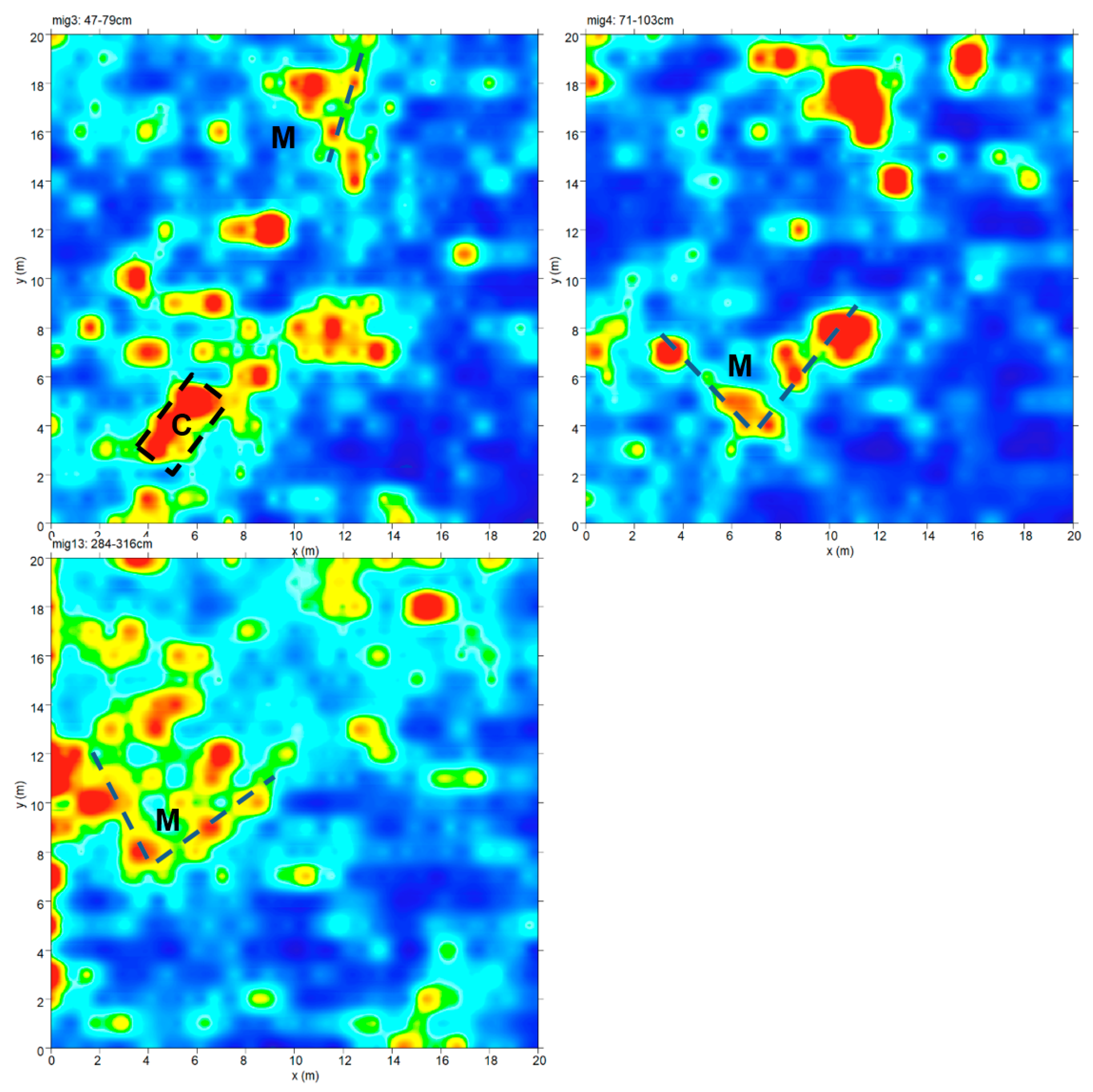
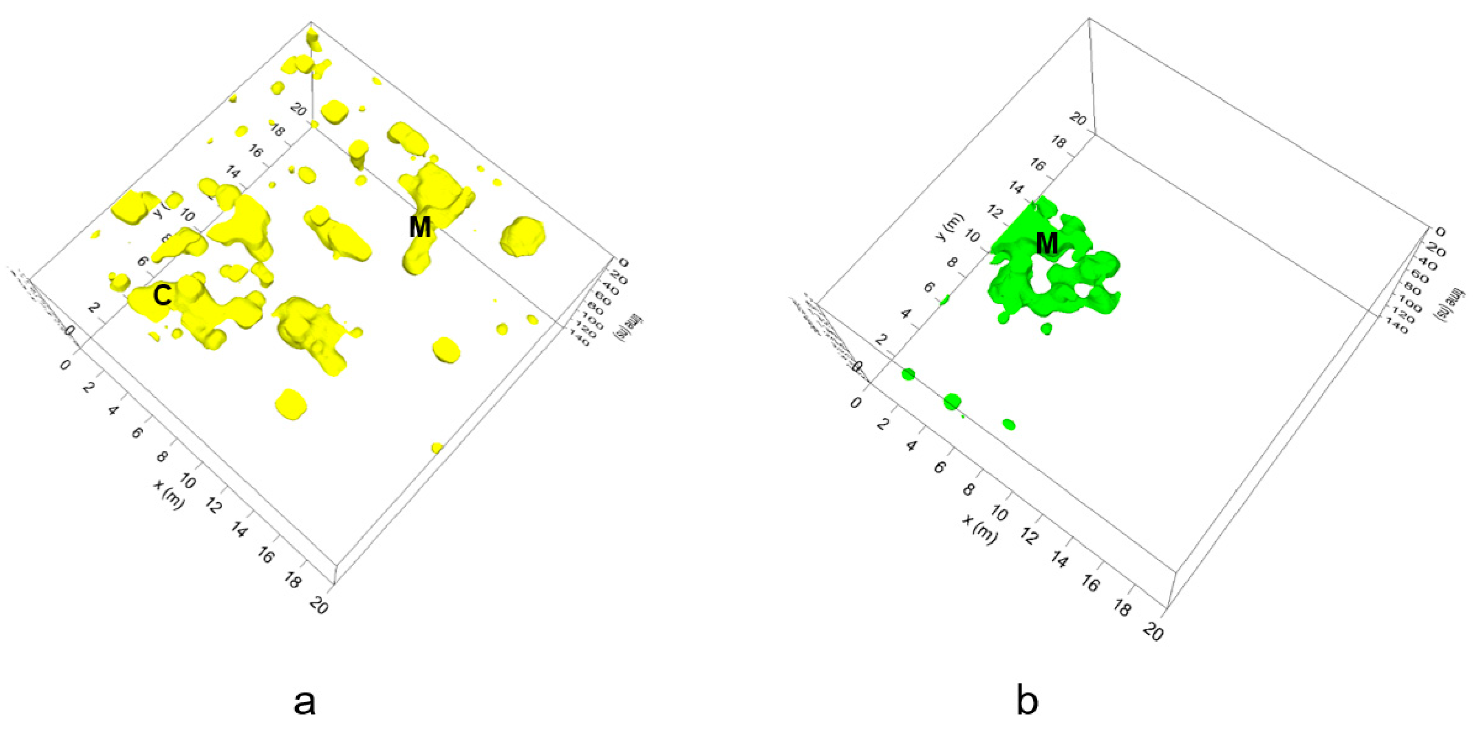
4.2.2. Zone 2: Area F, GPR Data Analysis
5. Archaeological Excavations
5.1. Archaeological Excavations in Zone 1
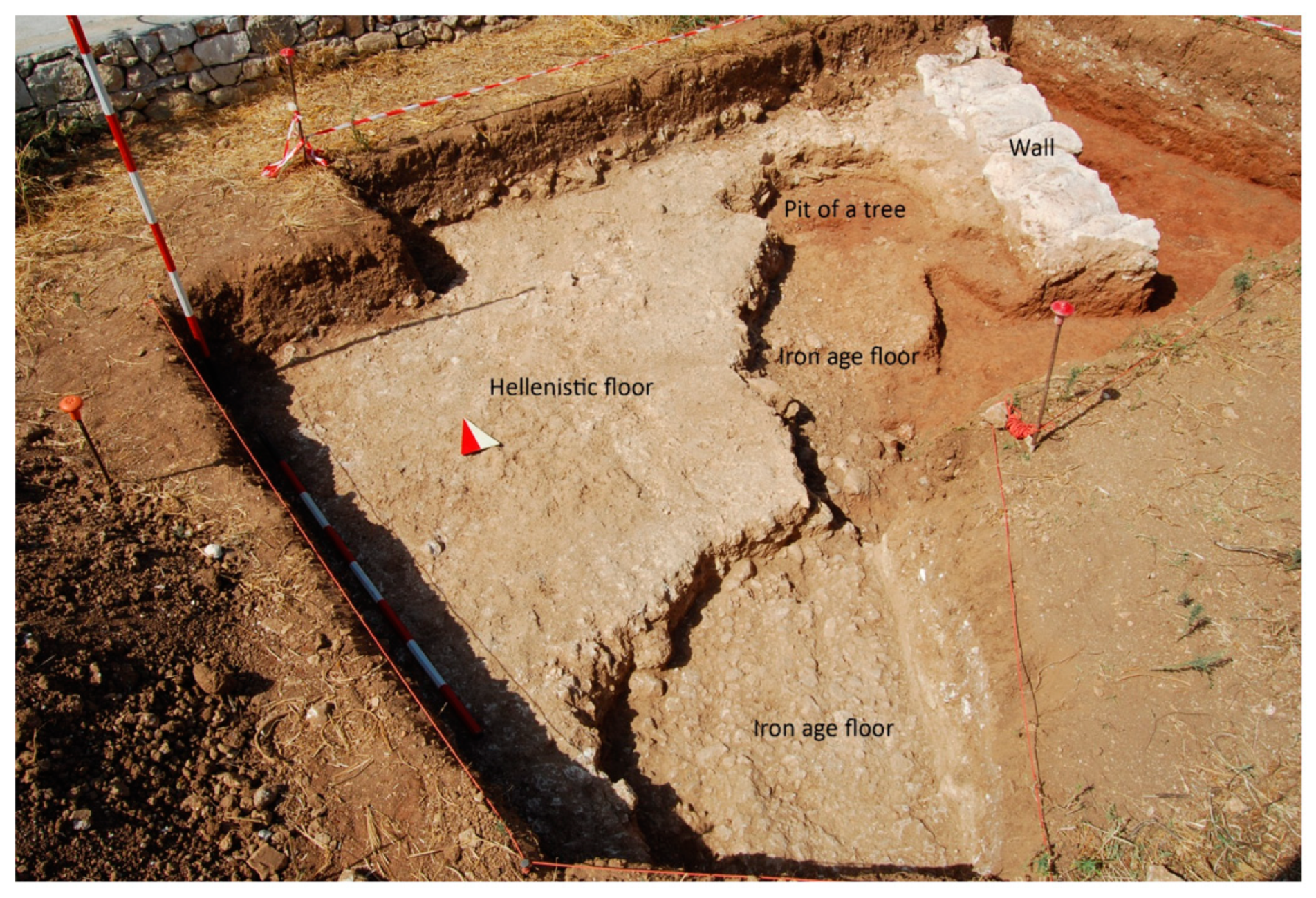
5.1.1. Excavation in Area B
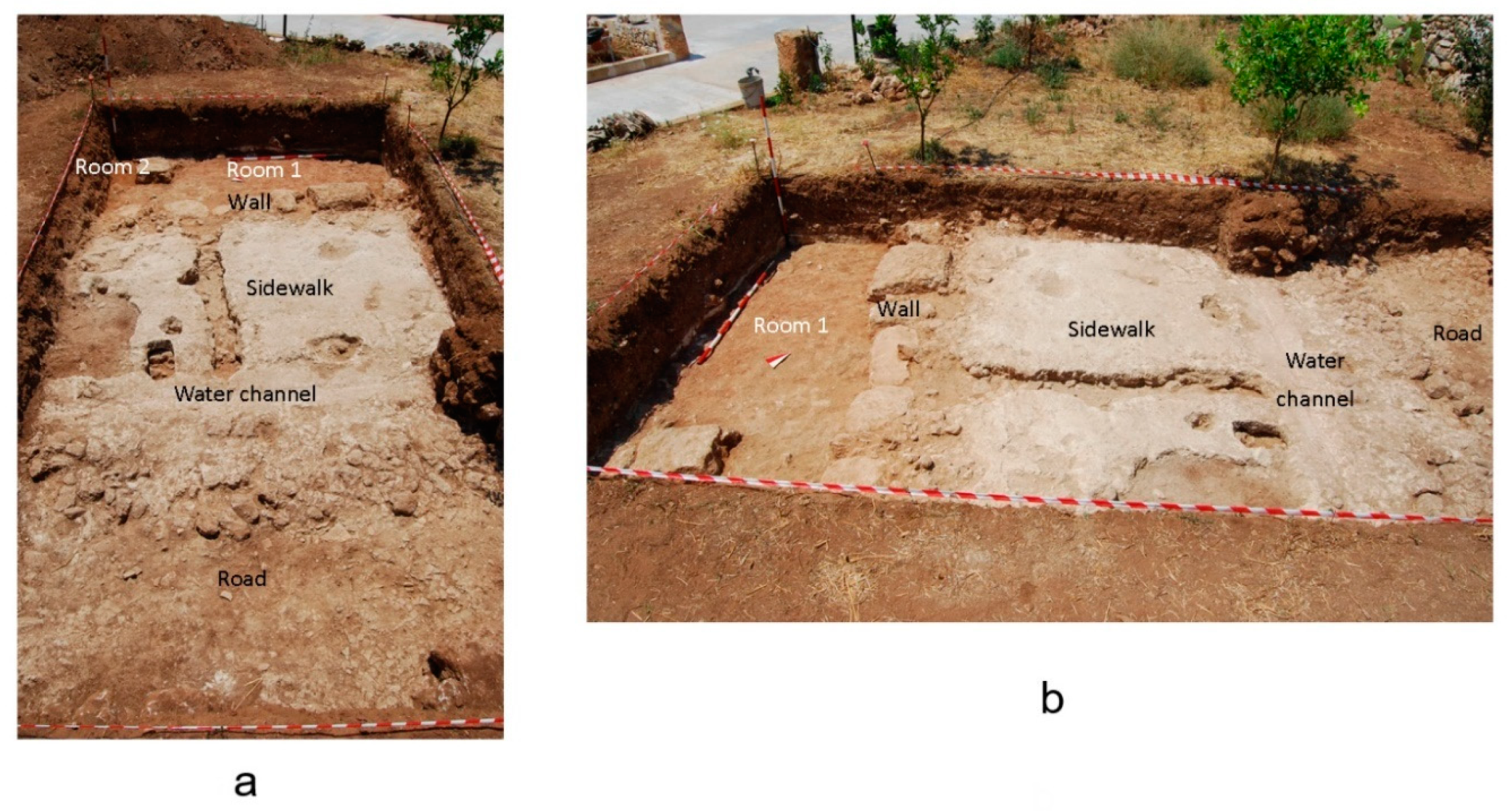
5.1.2. Excavation in Area E
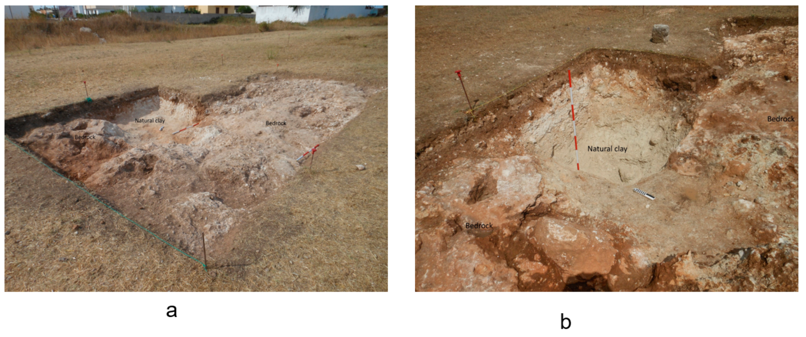
5.2. Archaeological Excavation in Zone 2
6. Discussion and Conclusions
Author Contributions
Funding
Conflicts of Interest
References
- De Giorgi, L.; Leucci, G. Study of Shallow Low-Enthalpy Geothermal Resources Using Integrated Geophysical Methods. Acta Geophys. 2015, 63, 125–153. [Google Scholar] [CrossRef] [Green Version]
- Leucci, G.; De Giorgi, L. Microgravimetric and ground penetrating radar geophysical methods to map the shallow karstic cavities network in a coastal area (Marina di Capilungo, Lecce—Italy). Explor. Geophys. 2010, 41, 178–188. [Google Scholar] [CrossRef]
- Leucci, G. Ground Penetrating Radar a Useful Tool for Shallow Subsurface Stratigraphy Characterization; Intech: Rijeka, Croatia, 2012; ISBN 979-953-307-339-1. [Google Scholar]
- Furman, A.; Ferré, T.P.A.; Warrick, A.W. Optimization of ERT surveys for monitoring transient hydrological events using perturbation sensitivity and genetic algorithms. Vadose Zone J. 2004, 3, 1230–1239. [Google Scholar] [CrossRef]
- Leucci, G.; De Giorgi, L.; Gizzi, F.T.; Persico, R. Integrated geo-scientific surveys in the historical centre of Mesagne (Brindisi, Southern Italy). Nat. Hazards 2017, 86, 363–383. [Google Scholar] [CrossRef]
- Slater, L.; Binley, A.; Reeve, A. Solute transport processes in peat inferred from electrical imaging. In Proceedings of the Symposium on the Application of Geophysics to Environmental & Engineering Problems (SAGEEP 2003), San Antonio, TX, USA, 6–10 April 2003; pp. 676–686. [Google Scholar]
- Slater, L.; Glaser, D.; Utne, J.I.; Binley, A. Electrical imaging of permeable reactive barrier integrity. In Proceedings of the Symposium on the Application of Geophysics to Environmental & Engineering Problems (SAGEEP), Las Vegas, NE, USA, 10–14 February 2002. 10p. [Google Scholar]
- Dahlin, T.; Bernstone, C.; Loke, M.H. A 3-D resistivity investigation of a contaminated site at Lernacken, Sweden. Geophysics 2002, 67, 1692–1700. [Google Scholar] [CrossRef]
- Nowroozi, A.A.; Horrocks, S.B.; Henderson, B. Saltwater intrusion into the freshwater aquifer in the eastern shore of Virginia: A reconnaissance electrical resistivity survey. J. Appl. Geophys. 1999, 42, 1–22. [Google Scholar] [CrossRef]
- Van Schoor, A. Detection of sinkholes using 2D electrical resistivity imaging. J. Appl. Geophys. 2002, 50, 393–399. [Google Scholar] [CrossRef] [Green Version]
- Brunner, I.; Friedel, S.; Jacobs, F.; Danckwardt, E. Investigation of a Tertiary maar structure using three-dimensional resistivity imaging. Geophys. J. Int. 1999, 136, 771–780. [Google Scholar] [CrossRef] [Green Version]
- Giannino, F.; Leucci, G.; Teramo, A.; De Domenico, D. Geophysical Surveys to Improve the Knowledge on the S. Salvatore Fortress Structure (Messina, Italy); Atti del 24° Convegno Nazionale del GNGTS: Rome, Italy, 2005. [Google Scholar]
- Godio, A.; Strobbia, C.; De Bacco, G. Geophysical characterisation of a rockslide in an alpine region. Eng. Geol. 2006, 83, 273–286. [Google Scholar] [CrossRef]
- Leucci, G. The use of GPR to estimate volumetric water content and reinforced bar diameter in Concrete Structures. J. Adv. Concr. Technol. 2012, 10, 411–422. [Google Scholar] [CrossRef]
- Argote-Espino, D.; Tejero-Andrade, A.; Cifuentes-Nava, G.; Iriarte, L.; Farıas, S.; Chavez, R.E.; Lopez, F. 3D electrical prospection in the archaeological site El Pahnu, Hidalgo State, Central Mexico. J. Archaeol. Sci. 2013, 40, 1213–1223. [Google Scholar] [CrossRef]
- Aspinall, A.; Gaffney, C.F. The Schlumberger array-potential and pitfalls in archaeological prospection. Archaeol. Prospect. 2001, 8, 199–209. [Google Scholar] [CrossRef]
- Aspinall, A.; Gaffney, C.; Schmidt, A. Magnetometry for Archaeologists; Altamira Press: New York, NY, USA, 2009; p. 208. [Google Scholar]
- Goodman, D.; Piro, S. GPR Remote Sensing in Archaeology; Geotechnologies and the Environment Series; Springer-Verlag: Berlin, Germany, 2013; Volume 9, p. 233. [Google Scholar]
- Leucci, G. Geofisica Applicata All’archeologia e ai Beni Monumentali; Dario Faccovio Editore: Palermo, Italy, 2015; p. 368. [Google Scholar]
- Leucci, G. Nondestructive Testing for Archaeology and Cultural Heritage: A Practical Guide and New Perspective; Springer Nature Switzerland: Basel, Switzerland, 2019; p. 217. ISBN 978-3-030-01898-6. [Google Scholar]
- Leucci, G.; Parise, M.; Sammarco, M.; Scardozzi, G. The use of Geophysical prospections to map ancient hydraulic works: The Triglio underground aqueduct (Apulia, southern Italy). Archaeol. Prospect. 2016, 23, 195–211. [Google Scholar] [CrossRef]
- De Domenico, D.; Giannino, F.; Leucci, G.; Bottari, C. Integrated geophysical surveys at the archaeological site of Tindari (Sicily, Italy). J. Archaeol. Sci. 2006, 33, 961–970. [Google Scholar] [CrossRef]
- Gabellone, F.; Leucci, G.; Masini, N.; Persico, R.; Quarta, G.; Grasso, F. Nondestructive Prospecting and virtual reconstruction of the chapel of the Holy Spirit in Lecce, Italy. Near Surf. Geophys. 2013, 11, 231–238. [Google Scholar]
- Osella, A.; de la Vega, M.; Lascano, E. 3D electrical imaging of an archaeological site using electrical and electromagnetic methods. Geophysics 2005, 4, 101–107. [Google Scholar] [CrossRef]
- Persico, R.; Ciminale, M.; Matera, L. A new reconfigurable stepped frequency GPR system, possibilities and issues; applications to two different Cultural Heritage Resources. Near Surf. Geophys. 2014, 12, 793–801. [Google Scholar] [CrossRef]
- Conyers, L.B.; Goodman, D. Ground-Penetrating Radar—An Introduction for Archaeologists; AltaMira Press: New York, NY, USA, 1997; p. 232. [Google Scholar]
- Conyers, L.B. Ground-Penetrating Radar for Archaeology; Altamira Press: Walnut Creek, CA, USA, 2004; p. 224. [Google Scholar]
- Conyers, L.B. Ground-Penetrating Radar for Archaeology, 3rd ed.; Alta Mira Press: Walnut Creek, CA, USA, 2013; p. 258. [Google Scholar]
- Persico, R. An Introduction to Ground Penetrating Radar: Inverse Scattering and Data Processing; Wiley: Hoboken, NJ, USA, 2014; p. 368. [Google Scholar]
- Tejero-Andrade, A.; Cifuentes, G.; Chavez, R.E.; Lopez Gonzalez, A.; Delgado-Solorzano, C. “L” and ‘‘Corner’’ arrays for 3D electrical resistivity tomography: An alternative for urban zones. Near Surf. Geophys. 2015, 13, 1–13. [Google Scholar] [CrossRef]
- Conyers, L.B. Innovative ground-penetrating radar methods for archaeological mapping. Archaeol. Prospect. 2006, 13, 139–141. [Google Scholar] [CrossRef]
- Negri, S.; Leucci, G.; Mazzone, F. High resolution 3d ert to help gpr data interpretation for researching archaeological items in a geologically complex subsurface. J. Appl. Geophys. 2008, 65, 111–120. [Google Scholar] [CrossRef]
- Giardino, L.; Meo, F. Muro Leccese. I Segreti di una Città Messapica; Edizioni Grifo: Lecce, Italy, 2016. [Google Scholar]
- Meo, F. Muro Leccese nell’età del Ferro. Forma e organizzazione insediativa di un abitato indigeno della Puglia meridionale. MEFRA 2019, in press. [Google Scholar]
- Giardino, L. I gruppi gentilizi. In Muro Leccese. I Segreti di una Città MESSAPICA; Giardino, L., Meo, F., Eds.; Edizioni Grifo: Lecce, Italy, 2016; pp. 69–76. [Google Scholar]
- Giardino, L.; Meo, F. The Messapian Settlement of Muro Leccese in the Archaic period. Transformations and continuities. In Archaic Settlements in Southern Italy and Sicily, Proceedings of the International Conference Cavallino, Cavallino, Italy, 26–27 March 2015; Edipuglia: Bari, Italy, in press.
- Meo, F. La vita quotidiana nella città messapica. In Muro Leccese. I Segreti di una Città Messapica; Edizioni Grifo: Lecce, Italy, 2016; pp. 61–68. [Google Scholar]
- Bianco, C. La cinta muraria. In Muro Leccese. I Segreti di una Città Messapica; Edizioni Grifo: Lecce, Italy, 2016; pp. 101–108. [Google Scholar]
- Giardino, L.; Meo, F. L’area archeologica in località Cunella. In Muro Leccese. I Segreti di una Città Messapica; Edizioni Grifo: Lecce, Italy, 2016; pp. 109–115. [Google Scholar]
- Calvaruso, T.O. Le sepolture di età messapica: La documentazione archeologica. In Muro Leccese. I segreti di una città messapica; Edizioni Grifo: Lecce, Italy, 2016; pp. 83–90. [Google Scholar]
- Giardino, L. Cratere a volute attico a figure nere dal centro messapico di Muro Leccese (Puglia, Italia). In Le Cratère à Volutes. Destination d’un Vase de Prestige Entre Grecs et Non-Grecs; Cahiers du CVA 2; Académie des Inscriptions et Belles-Lettres: Paris, France, 2014; pp. 215–223. [Google Scholar]
- Lonoce, N. Le sepolture di età messapica: La documentazione antropologica. In Muro Leccese. I segreti di una città messapica; Edizioni Grifo: Lecce, Italy, 2016; pp. 91–97. [Google Scholar]
- Goodman, D. GPR Sim Manual. Available online: http://www.gprsurvey.com (accessed on 7 May 2019).
- Chavez, G.; Tejero, A.; Alcantara, M.A.; Chavez, R.E. The ‘L-Array’, a tool to characterize a fracture pattern in an urban zone: In expanded abstracts: Near surface. Eur. Assoc. Geosci. Eng. 2011, 1, 114–155. [Google Scholar]
- Goodman, D.; Steinberg, J.; Damiata, B.; Nishimure, Y.; Schneider, K.; Hiromichi, H.; Hisashi, N. GPR overlay analysis for archaeological prospection. In Proceedings of the 11th International Conference on Ground Penetrating Radar, Columbus, OH, USA, 19–22 June 2006. [Google Scholar]
- Leucci, G.; Masini, N.; Persico, R.; Soldovieri, F. GPR and sonic tomography for structural restoration: The case of the Cathedral of Tricarico. J. Geophys. Eng. 2011, 8, S76–S92. [Google Scholar] [CrossRef]
- Giardino, L.; Meo, F. Attestazioni di pratiche rituali di età arcaica nell’abitato messapico di Muro Leccese (Le). In Archeologia dei Luoghi e Delle Pratiche di Culto. Atti del Convegno (Cavallino, 26–27 Gennaio 2012); Edipuglia: Bari, Italy, 2013; pp. 165–203. [Google Scholar]
- Giardino, L. Muro Leccese. La città messapica senza nome. In Libro di Pasquale Maggiulli 1992 al Parco Archeologico Del 2000; Edizioni Goffreda: Maglie (Lecce), Italy, 2002. [Google Scholar]
- Giardino, L.; Meo, F. Un decennio di indagini archeologiche a Muro Leccese. Il villaggio dell’età del Ferro e l’abitato arcaico. In Vetustis Novitatem Dare. Temi di Antichità e Archeologia in Ricordo di Grazia Angela Maruggi; Scorpione Editrice: Taranto, Italy, 2013; pp. 299–319. [Google Scholar]
- Meo, F. Birth and Transformation of a Messapian Settlement from the Iron Age to the Classical Period. The Example of Muro Leccese. In Making Cities, Economies of Production and Urbanisation in Mediterranean Europe 1000-500 BCE, Proceedings of the International Symposium, Cambridge, UK, 18–19 May 2017; Cambridge University Press: Cambridge, UK, 2019; in press. [Google Scholar]


© 2019 by the authors. Licensee MDPI, Basel, Switzerland. This article is an open access article distributed under the terms and conditions of the Creative Commons Attribution (CC BY) license (http://creativecommons.org/licenses/by/4.0/).
Share and Cite
Bianco, C.; De Giorgi, L.; Giannotta, M.T.; Leucci, G.; Meo, F.; Persico, R. The Messapic Site of Muro Leccese: New Results from Integrated Geophysical and Archaeological Surveys. Remote Sens. 2019, 11, 1478. https://0-doi-org.brum.beds.ac.uk/10.3390/rs11121478
Bianco C, De Giorgi L, Giannotta MT, Leucci G, Meo F, Persico R. The Messapic Site of Muro Leccese: New Results from Integrated Geophysical and Archaeological Surveys. Remote Sensing. 2019; 11(12):1478. https://0-doi-org.brum.beds.ac.uk/10.3390/rs11121478
Chicago/Turabian StyleBianco, Catia, Lara De Giorgi, Maria T. Giannotta, Giovanni Leucci, Francesco Meo, and Raffaele Persico. 2019. "The Messapic Site of Muro Leccese: New Results from Integrated Geophysical and Archaeological Surveys" Remote Sensing 11, no. 12: 1478. https://0-doi-org.brum.beds.ac.uk/10.3390/rs11121478