Quantifying Leaf Phenology of Individual Trees and Species in a Tropical Forest Using Unmanned Aerial Vehicle (UAV) Images

Abstract

Tropical forests exhibit complex but poorly understood patterns of leaf phenology. Understanding species- and individual-level phenological patterns in tropical forests requires datasets covering large numbers of trees, which can be provided by Unmanned Aerial Vehicles (UAVs). In this paper, we test a workflow combining high-resolution RGB images (7 cm/pixel) acquired from UAVs with a machine learning algorithm to monitor tree and species leaf phenology in a tropical forest in Panama. We acquired images for 34 flight dates over a 12-month period. Crown boundaries were digitized in images and linked with forest inventory data to identify species. We evaluated predictions of leaf cover from different models that included up to 14 image features extracted for each crown on each date. The models were trained and tested with visual estimates of leaf cover from 2422 images from 85 crowns belonging to eight species spanning a range of phenological patterns. The best-performing model included both standard color metrics, as well as texture metrics that quantify within-crown variation, with r² of 0.84 and mean absolute error (MAE) of 7.8% in 10-fold cross-validation. In contrast, the model based only on the widely-used Green Chromatic Coordinate (GCC) index performed relatively poorly (r² = 0.52, MAE = 13.6%). These results highlight the utility of texture features for image analysis of tropical forest canopies, where illumination changes may diminish the utility of color indices, such as GCC. The algorithm successfully predicted both individual-tree and species patterns, with mean r² of 0.82 and 0.89 and mean MAE of 8.1% and 6.0% for individual- and species-level analyses, respectively. Our study is the first to develop and test methods for landscape-scale UAV monitoring of individual trees and species in diverse tropical forests. Our analyses revealed undescribed patterns of high intraspecific variation and complex leaf cover changes for some species.

1. Introduction

Plant phenology has long been recognized as a critical driver of ecosystem processes, and one heavily influenced by climate. Satellite observations and field data have provided high confidence that phenological shifts have been caused by climate change in recent decades in temperate and boreal ecosystems [1]. Compared to temperate and boreal ecosystems, however, relatively little is known about the leaf phenology of tropical forests, how it responds to climate variability, and how phenological shifts might impact tropical forest ecosystems [2,3]. Tropical forests have many more tree species than temperate forests, and tropical species exhibit a much greater variety of phenological patterns, including species that are entirely leafless for several months, species that partially lose their leaves for an extended time, species that drop and flush leaves quickly, species with continuous leaf turnover throughout the year, and species with two periods of leaf drop and leaf flush, with multiple types often present within a given site [4,5]. To better understand the potential drivers of variation in tropical tree leaf phenology, a critical first step is to quantify patterns in tropical forest phenology at individual and species levels. However, few datasets have the combination of high spatial and temporal resolution and comprehensive coverage needed to quantify intra- and interspecific variation in tropical leaf phenology, which requires individual tree-level monitoring for many species.

Commonly used field methods and satellite remote sensing have provided important insights for tropical forest phenology, but have difficulty capturing leaf phenology patterns among and within species on a landscape scale. Field observations, such as scoring tree crowns for leaf presence or cover [6,7,8,9], are useful for individual tree-level monitoring, but are very labor-intensive. In addition, it can be difficult for an observer on the ground to make accurate assessments of the upper canopy in tall, dense, multi-layered forests. Litter traps can provide long-term information on species- and stand-level leaf-fall [10,11], but this method provides limited information on intraspecific variation and no information about the timing of leaf flush. Satellite images, which have been used successfully in temperate and boreal areas to document phenology patterns and their shifts in response to climate, are more difficult to interpret in tropical areas. Frequent cloud cover, smoke from fires and haze, and sensor artifacts complicate satellite-based studies of tropical forest phenology [12], which has led to ongoing debate concerning the patterns of phenology in areas such as the Amazon [13,14,15,16]. Furthermore, the spatial scale of satellite images allows tracking of at best only the largest canopy trees, thus precluding individual- or species-level measurements for all but a few species [17,18].

Near-surface remote sensing, such as tower-mounted cameras (“phenocams”), have provided important next steps in quantifying tropical forest leaf phenology. Phenocams can quantify leaf phenology for multiple individual crowns with high frequency (every 30 min) without being obscured by clouds [15,19]. Analyses of phenocam images of a 4-ha area in the Amazon showed that the majority of crowns flush new leaves during the dry season, providing support for some satellite-based studies that indicate Amazon forests “green up” in the dry season [15]. The frequent temporal sampling of phenocams allows the selection of cloud-free images with consistent atmospheric conditions and fixed viewing geometry to quantify changes in the color of crowns related to leaf cover changes. However, in species-rich forests, the limited area covered by phenocams provides insufficient sample sizes for studying intra- and interspecific variation of leaf phenology. Furthermore, most individual crowns are not georeferenced in phenocam images, making it difficult to link these crowns to specific trees on the ground for which field data, including species identification, have been recorded [15,19].

Unmanned aerial vehicles (UAVs) are another form of near-surface remote sensing that can potentially provide important advances in monitoring tropical forest phenology. UAV images can cover areas ranging from many hectares to many square kilometers, thus encompassing enough trees to provide large sample sizes for many species. Since UAV images view crowns directly from above and can be georeferenced, trees in UAV images can be linked with trees on the ground so that data on species identity, stem diameter, growth rate, physiological measurements, and micro-environmental conditions can be associated with each crown in the image. Phenological studies using UAVs in a temperate forest have used individual color-channel indices (Green and Blue Chromatic Coordinates, GCC and BCC) from image time-series, taken under cloud-free conditions, to quantify the contribution of individual species to landscape patterns of phenology [20,21]. Unfortunately, in many tropical forest regions, opportunities for cloud-free flights are too infrequent to develop full-year time-series under consistent atmospheric conditions, which may limit the utility of simple color metrics such as GCC. As with satellite data, near-surface images of tropical forests are affected by highly variable solar conditions, frequent cloud shadows, and mist that hangs over the canopy. Therefore, a key challenge for using UAV images to monitor tropical forest leaf phenology is to develop methods to extract accurate quantitative phenology estimates under variable lighting and viewing conditions.

An alternative approach to using simple color indices (e.g., GCC) is to capitalize on the wealth of detail in fine-resolution (e.g., <10 cm) UAV images, which can be used to quantify variation or “texture” within tree crowns [22]. Remote-sensing texture metrics have been used to analyze patterns in ecosystem characteristics such as species richness [23,24,25], but have not been used for phenological studies. Even under variable lighting conditions, a human interpreter can easily recognize changes in leaf cover of canopy trees in a fine-resolution UAV image time-series. Leafless crowns, which have exposed branches, shadows between branches, and upwelling radiation from understory trees beneath the upper canopy, have high within-crown variation in color. In contrast, fully-leaved crowns have mostly green leaves, little to no exposed branches and fewer shadows, and therefore less within-crown color variability. Therefore, texture-based image features that quantify within-crown color variation [22] may be sensitive to changes in leaf cover, even under highly variable lighting conditions.

In this study, we propose and test methods for quantifying leaf phenology of individual tree crowns in tropical forests using UAV image time-series. Our study is the first to develop and test methods suitable for landscape-scale monitoring of individual trees and species in diverse tropical forests. We used percent leaf cover (or “leaf cover”), the two-dimensional coverage of green leaves, for quantifying leaf phenology of tree crowns. Leaf cover has been often used in field-based studies of leaf phenology [6,9], but little used in remote sensing to this point. Percent leaf cover is similar to, but at a finer spatial scale than % canopy or crown cover [26,27], or the spatial coverage of green tree canopies, which are more widely used in remote-sensing studies. Although percent leaf cover limits our study to the two-dimensional coverage of leaves in the upper canopy, assessing three-dimensional leaf distributions would require understanding the seasonal change of leaf position across vertical structure of tree crowns, which is beyond the scope of this study. Our methodology uses a machine learning approach, in which observations (human-interpreted estimates of leaf cover in image time-series) for individual tree crowns are used to train statistical models that predict leaf cover from color and texture features. We quantify how well our method captures seasonal patterns of leaf cover for individual trees and species, and how model performance depends on the types of image features (color and/or texture indices) included in the model. We evaluate model performance based on prediction errors for out-of-sample observations (i.e., observations excluded from training data) for a variety of data subsets, including 10-fold cross-validation, out-of-sample individual trees, out-of-sample species, and out-of-sample time periods. We also evaluate the repeatability of human image interpretation. We show that in our study, visual estimates of leaf cover are largely repeatable among different human observers, and that model predictions are insensitive to modest differences among observers.

2. Materials and Methods

2.1. Study Site and Ground-Based Forest Inventory Data

This study was conducted in the 50-ha forest dynamics plot in lowland moist tropical forest on Barro Colorado Island (9°9′12.002″ N, 79°51′2.491″ W) in the Republic of Panama. The 50-ha plot (1000 m × 500 m) is the site of a long-term forest dynamics monitoring effort in which every tree ≥ 1 cm in DBH (diameter at breast height, 1.3 m) is tagged, identified to species, and recensused every 5 years since 1985 [28]. As explained below, we matched individual crowns in UAV images to trees in the 50-ha plot, so that the species identity of each crown was known. Mean annual rainfall at the site was 2657 mm (SD = 478 mm) for the period 1929 to 2017, with a pronounced dry season from mid-December to mid-April when many trees lose some or all of their leaves [29].

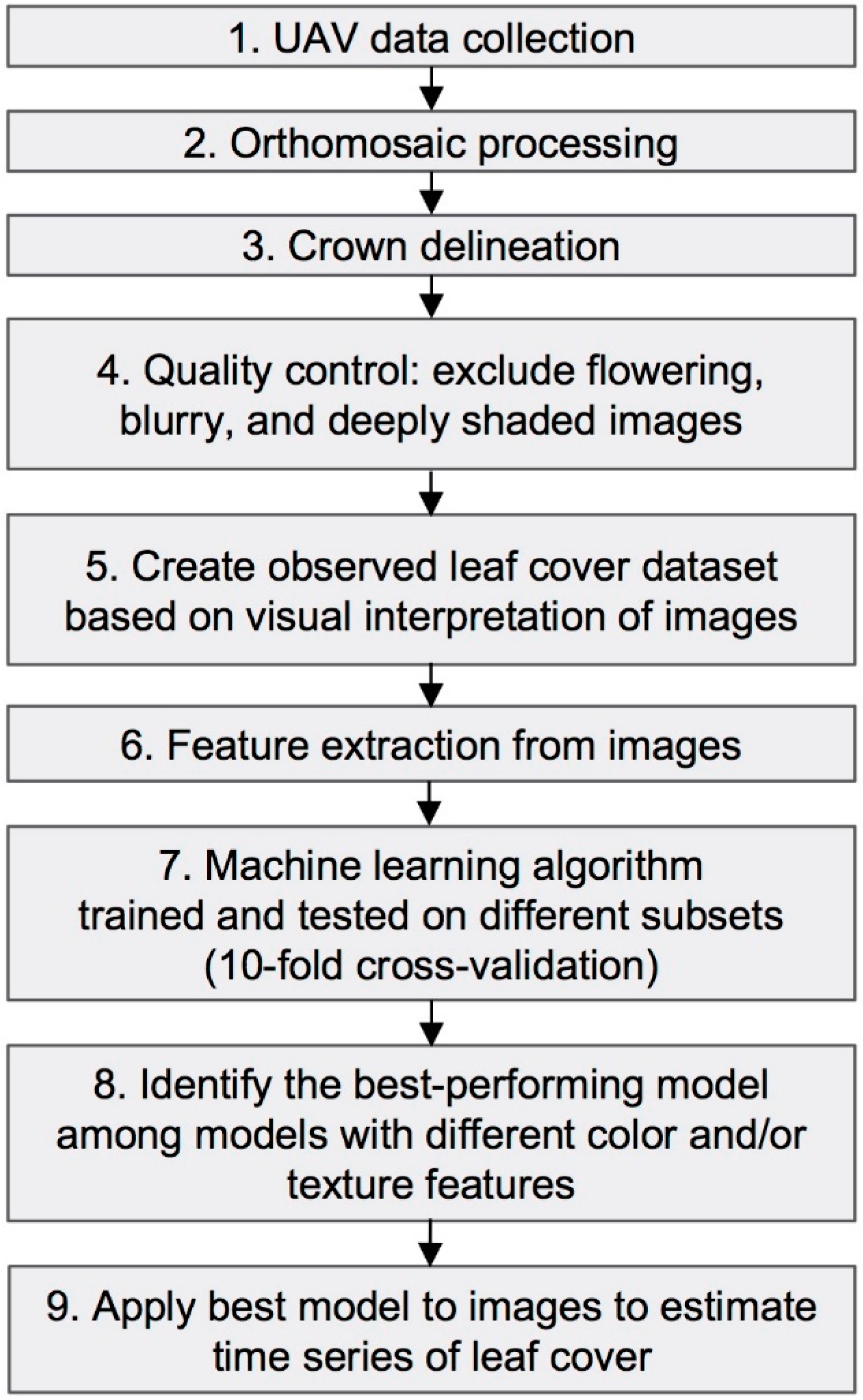
2.2. Overview of UAV Image Acquisition and Analysis

We collected and processed one year of weekly to biweekly aerial images (34 image sets from 2 October 2014 to 30 September 2015) to quantify intra-annual patterns of variation in leaf cover of individual trees and species. We manually delineated boundaries of individual tree crowns based on the 2 October 2014 orthomosaic image, then used ground surveys to link each crown to a tagged tree in the 50-ha plot. After quality control, we created a training and testing dataset for a machine learning algorithm by visually interpreting leaf cover for 2422 images of 85 tree crowns on 34 dates. We used the machine learning algorithm to develop alternative models based on different sets of color and/or texture features extracted from each image. The best-performing model was then applied to all images for subsequent analyses, including evaluating model performance for individual dates, as well as annual patterns of leaf cover for individual trees and species. The workflow is presented in Figure 1.

2.3. UAV Flights and Image Processing

Here, we provide a brief description of image collection and processing methods; additional explanation and details are in Appendix A. UAV remote sensing was carried out with a consumer-grade multirotor aircraft equipped with the Pixhawk flight controller (3DRobotics Inc.; http://copter.ardupilot.com) and configured for automated waypoint flight. The multirotor design was based on previous work [30,31]. Missions were flown approximately every week from 2 October 2014 to 1 June 2015 and then approximately every two weeks from 1 June 2015 to 30 September 2015. The camera was calibrated for every flight to reduce effects from variable illumination within and among flights. Post-collection image processing to further reduce variability across color channels involved radiometric normalization of the image set using pseudo-invariant features and histogram equalization techniques. Radiometrically normalized image sets were processed into 7-cm resolution georeferenced orthomosaics using Agisoft Photoscan Professional (64-bit, v1.1.6, build 2038). Due to the relatively low accuracy of the UAV’s on-board GPS, the orthomosaics showed large horizontal georeferencing errors (>5 m) relative to existing LIDAR digital surface model in this area from 2009 [32]; therefore, horizontal georeferencing was performed manually in ArcGIS relative to the high-resolution LIDAR digital surface model from 2009 to reduce the errors (<1 m). An example of a full orthomosaic image is shown in Figure 2.

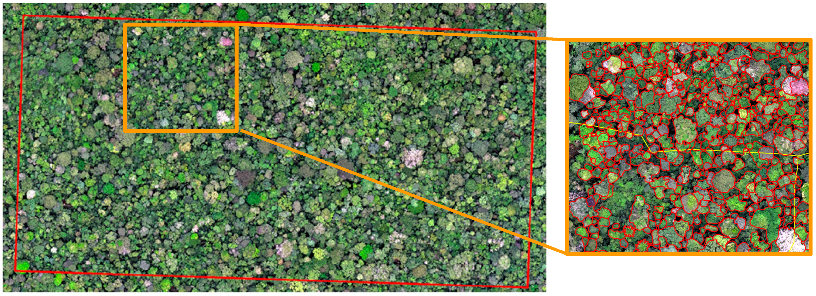
2.4. Manual Tree Crown Delineation

We linked delineated crowns in the images to stems in the 50 ha forest inventory plot using methods described in References [33,34] as follows. Within the 50-ha plot, we manually delineated boundaries of all individual tree crowns with an area greater than 50 m² (crown area based on the 2 October 2014 orthomosaic image), as well as some tree crowns smaller than 50 m² that were distinct enough in images to delineate. We then used ground surveys to link each crown to a tagged tree in the 50-ha plot. The crown polygon map, tree stem locations, and orthomosaic were loaded on a tablet, which was used in the field to match each crown polygon to a tagged tree. The total number of crowns digitized and linked to tagged trees was 2133, but we only use a subset of these crowns in this paper as described below. Additional details on the digitizing and field procedures are described in Appendix A.

2.5. Quality Assessment of Images

For each crown, we created a time series of images by extracting the relevant area from each orthomosaic. For each crown, we collated these images into a “montage” (Figure 3) to facilitate visual assessment of changes over time. In the context of our analyses, “image” hereafter refers to the area within a crown polygon on a given date. We performed a visual quality assessment of all crown montages to remove problematic images. We removed images that had visible flower cover (0.5% of the total images) because the present study focuses only on leaf phenology, and the presence of flowers tended to result in an underestimation of leaf cover. We also removed crown montages for which we could not visually estimate leaf cover because the images were too blurry or deeply shadowed (22% of crown montages; Figure A1).

2.6. Statistical Analysis

2.6.1. Generating an Observation Dataset for the Machine Learning Algorithm

We used a subset of the quality-controlled crown montages to generate an observation dataset to train and test a machine learning algorithm. The subset analyzed in this paper included all quality-controlled images for 85 total individuals (2422 images) belonging to eight tree species that are known to be deciduous (

Table 1. Tropical tree species included in the training and testing dataset. N is the number of trees in the observation dataset for a given species.

Species Name	Abbreviation	N	Crown Area (m2) Mean (SD)	Min. Observed Leaf Cover (%) Mean (Range)	Mean Observed Leaf Cover (%) Mean (Range)	Max. Observed Leaf Cover (%) Mean (Range)
Cavanillesia platanifolia	CAVAPL	14	274 (171)	13 (5–30)	69 (53–92)	100 (100–100)
Ceiba pentandra	CIEBPE	10	1180 (414)	24 (10–52)	81 (72–93)	99 (95–100)
Cordia alliodora	CORDAL	8	102 (43)	20 (5–40)	71 (64–86)	99 (95–100)
Platypodium elegans	PLA2EL	14	188 (51)	12 (0–70)	75 (53–96)	100 (100–100)
Sterculia apetala	STERAP	10	261 (116)	14 (0–50)	93 (85–98)	100 (100–100)
Handroanthus guayacan	TAB1GU	9	193 (40)	18 (0–45)	79 (63–92)	99 (95–100)
Tabebuia rosea	TAB1RO	10	146 (55)	3 (0–15)	65 (33–75)	99 (85–100)
Zanthoxylum ekmanii	ZANTBE	10	211 (38)	16 (5–35)	85 (79–93)	100 (100–100)

). We focused on deciduous species in order to provide a wide range of percent leaf cover for model training and testing. To create an observation dataset, human observers visually interpreted each image to estimate percent leaf cover (e.g., Figure 3). As with ground-based visual estimates of percent leaf cover that are widely used to study leaf phenology in the tropics [6,7,8,9], visual interpretation of images is prone to human error. However, because UAV images provide an unobstructed view of the canopy from above, we expect errors in UAV image interpretation to be smaller than those associated with ground-based visual estimates (particularly in dense, multi-layered tropical forests). We evaluated the repeatability of leaf cover estimates among observers, as well as the sensitivity of our analysis to observer differences (for details, see Appendix A). Because repeatability was high (see Results), analyses presented in this paper are based on a single observer (unless stated otherwise). In estimating percent leaf cover, we did not distinguish between liana and host tree leaf cover. Therefore, the estimates included any leaves and branches that were present in the crown regardless of whether they originated from the host tree or a liana.

2.6.2. Feature Extraction from Images

For each image, we calculated 14 color and texture metrics (“features”;

Table 2. Color and texture features used to predict leaf cover of individual crowns. The full model included all 14 features, and other models included a subset of the features.

Feature Type	Crown-Level Statistic	Feature Name	Abbreviation	Pixel-Scale Transformations	References
Mean Color Indices	Mean	RGB Chromatic Coordinates (RCC, GCC, BCC)	RCCm	RCC = red/(green + red + blue)	[35]
			GCCm	GCC = green/(green + red + blue)
			BCCm	BCC = blue/(green + red + blue)
		Excess greenness	ExGm	ExG = 2*green − (red + blue)	[31]
		Green vegetation	GVm	From linear mixture model, each endmember fractions were calculated (shade-normalized), for more details see methods	[36]
		Non-photosynthetic vegetation	NPVm
Texture Indices	Standard deviation	RGB color indices	Rsd	Red (no transformation)	NA
			Gsd	Green (no transformation)
			Bsd	Blue (no transformation)
		Excess greenness	ExGsd	See above	Same as corresponding mean-based indices
		Green vegetation	GVsd
		Non-photosynthetic vegetation	NPVsd
		Grey-Level Co-Occurrence Matrix (GLCM) correlation	Gcor_sd	Moving window (5 by 5 pixels) was used to calculate GLCM correlation of a target region within a crown image	[37]
	Median		Gcor_md

), where “texture” can include a variety of metrics of variation within an image [22]. Because images for a given tree crown are not perfectly aligned across dates, we reduced each crown polygon by a 2-m buffer to ensure that features were derived only from the crown of interest. Below, we briefly describe the color and texture features. Additional details are in Appendix A.

Color features included Red, Green, and Blue Chromatic Coordinates (RCC, GCC, and BCC), Excess Green (ExG), and canopy surface fractions of green vegetation (GV) and non-photosynthetic vegetation (NPV) from endmember analysis. We calculated crown-level means of each color index (hereafter, “RCCm”, “GCCm”, and “BCCm”) for each image as in previous analyses of phenocam images [15].

Texture features included standard deviations of red, green, and blue channels and of ExG, NPV, and GV. We also derived two texture features from the Grey-Level Co-occurrence Matrix correlation (Gcor), which quantifies the similarity in grey levels among neighboring pixels within moving windows. We calculated Gcor within moving windows of 5 × 5 pixels (35 × 35 cm), and we then calculated the median and standard deviation of Gcor within each image (Gcor_md and Gcor_sd, respectively).

2.6.3. Model Training and Evaluation

To predict leaf cover of each crown polygon from different sets of the 14 color and texture features described above, we used stochastic gradient tree boosting (SGTB; [38]), a machine learning algorithm. Details on our implementation of SGTB are provided in Appendix A.

We compared alternative models incorporating some or all of the 14 crown features. We evaluated the performance of each model using K-fold cross-validation [39], which evaluates model performance based on “out-of-sample error” (i.e., how well the model fits validation data that were not used for training). Out-of-sample errors are particularly relevant for our study, because we are interested in developing and testing methodology that could in the future be applied to individuals, species, or time periods for which no training data are available. In contrast, AIC and related metrics are based on “in-sample error” (i.e., how well the model fits the training data) [39]. We used K = 10 (i.e., 10-fold cross-validation), which provides a good balance between variance (precision of predictions) and bias (accuracy of predictions) [39]. We implemented 10-fold cross-validation as follows: We randomly partitioned the observation data (2422 images) into 10 subsets, and used nine subsets (90% of observations) for training and one subset (10% of observations) for out-of-sample testing. For each model, we repeated this process 10 times, so that each subset was used nine times for model training and once for validation. This procedure provided one out-of-sample prediction for each observation.

In addition to 10-fold cross-validation, we performed additional analyses to explore how the amount and timing of training data affects model performance. These additional analyses included using the first half of the observations (2 October 2014 to 25 February 2015) for training and the second half (4 March 2015 to 30 September 2015) for validation; using the second half for training and the first half for validation; and alternating sequential sampling dates for training/validation.

To evaluate model performance, we used three goodness-of-fit metrics for out-of-sample predictions (i.e., all metrics were based on predictions for observations not included in training data): r², mean absolute error (MAE), and mean error (ME). r² is the squared Pearson correlation between observed and predicted leaf cover, which indicates the proportion of variance in leaf cover explained by the model. MAE and ME are defined as:

$$MAE=\frac{1}{N}{\displaystyle \sum }_{i=1}^N\left|ob{s}_i-pre{d}_i\right|$$

$$ME=\frac{1}{N}{\displaystyle \sum }_{i=1}^N\left(ob{s}_i-pre{d}_i\right)$$

where N is the number of images, and obs_i and pred_i are observed and predicted leaf cover of image i. Both MAE and ME have units of % leaf cover. MAE measures the magnitude of the deviations between predicted and observed leaf cover, whereas ME measures bias (systematic over- or under-prediction). Because the “full model” (including all 14 features) had the best goodness-of-fit metrics (see Results), we used the full model for subsequent analyses described below. Note that because goodness-of-fit metrics were based on out-of-sample predictions, the full model is not guaranteed a priori to have the best goodness-of-fit.

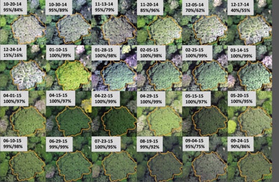
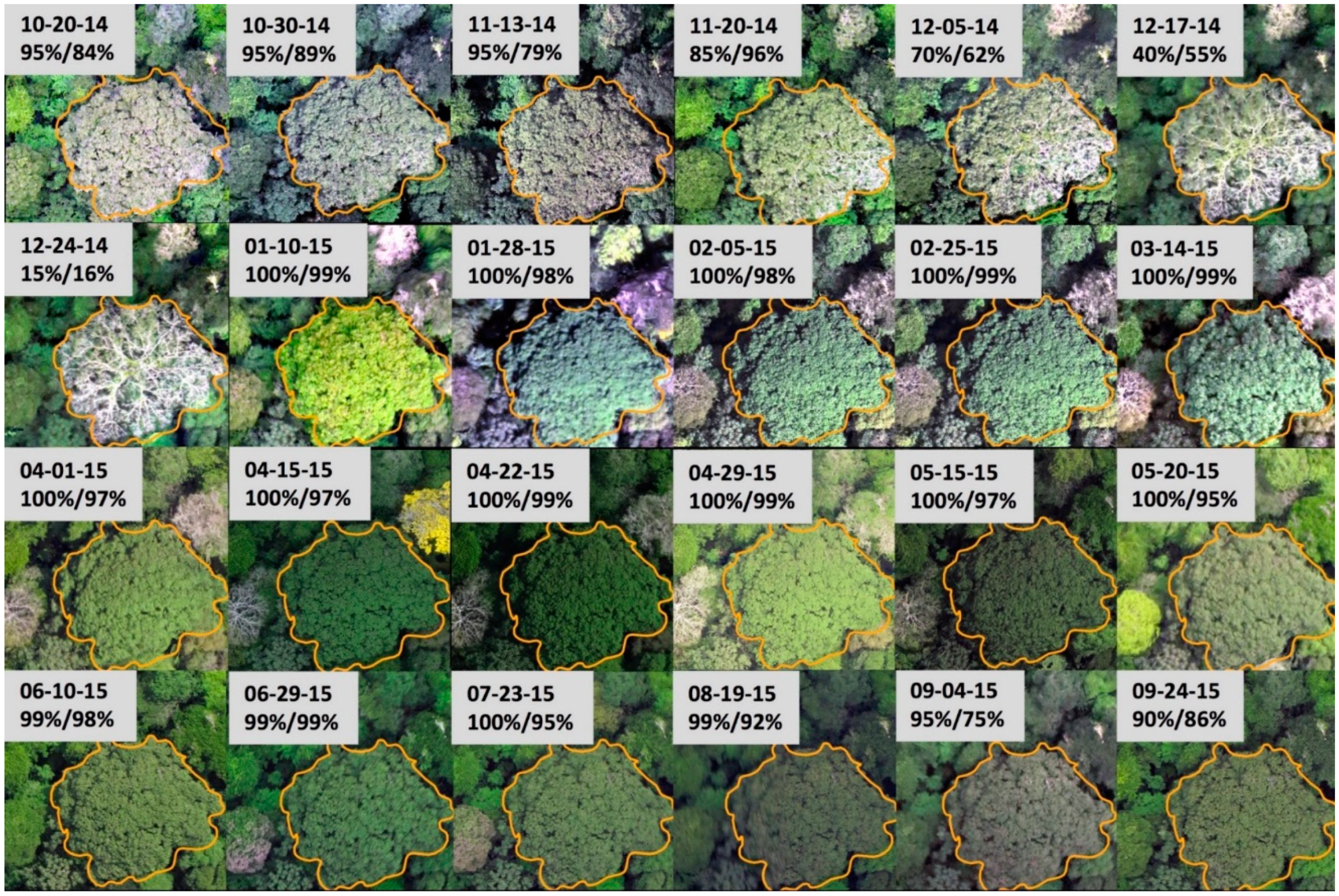
2.6.4. Evaluating Model Predictions of Intra-Annual Variation of Leaf Cover

Using the full model, we evaluated model predictions of intra-annual variation in leaf cover for the mean of all trees in the observation dataset on a given date, for individual species, and for individual trees. For the analysis of mean leaf cover, we used the out-of-sample prediction for each image from the 10-fold cross-validation procedure described above. We then calculated r² over time (34 sample dates) between the observed and predicted means. We also evaluated the r² over time between the observed means and GCCm (averaged over all trees on a given date), because GCCm is the most commonly used metric for quantifying canopy phenology in near-surface remote-sensing.

To evaluate how well the model captured intra-annual variation in leaf cover for a given species, we trained the model using observations for all species except the target (out-of-sample) species. We then generated species-level time-series of observed and predicted leaf cover by averaging over all crowns of the target species for each of the 34 sampling dates. We evaluated these species-level predictions using r², MAE, and ME. We repeated this process for each of the eight species in the observed dataset.

To evaluate how well the model captured intra-annual variation in leaf cover for a given individual tree, we trained the model on all observations except those of the target (out-of-sample) tree, and we then evaluated model predictions for the target tree for the 34 sampling dates. We evaluated these individual-level predictions using r², MAE, and ME. We repeated this analysis for each of the 85 individual trees in our observed dataset. To explore how individual tree properties might influence model performance, we regressed each goodness-of-fit metric (r² and MAE) on mean observed leaf cover (across the 34 sample dates for a given tree) and log-transformed crown area. The sample size for these regressions was the number of trees in our analysis (n = 85).

2.6.5. Evaluating Model Predictions

All model performance metrics (r², MAE, and ME) presented in this paper are based on out-of-sample predictions (i.e., predictions for observations excluded from training data for a given analysis). The data subset used to evaluate out-of-sample predictions differed among analyses. For 10-fold cross-validation used to compare the performance of models that include different predictor variables, out-of-sample observations were randomly selected (see details above). For split-dataset analyses (50% training, 50% validation), out-of-sample observations were from the first half of the study period, the second half, or from alternate dates. For individual tree- or species-level tests, out-of-sample observations belonged to a single tree or species.

3. Results

3.1. Comparing Models with Different Image Features

The best-performing model (based on 10-fold cross-validation) was the “full model” that included all 14 image features, including both color and texture features (r² = 0.84; MAE = 7.8%; ME = −0.07%;

Table 3. Comparison of models incorporating different combinations and numbers of features (additional models in Table A1). Goodness-of-fit statistics were calculated for out-of-sample data from 10-fold cross-validation. r² is the squared Pearson correlation. MAE and ME are mean absolute error and mean error, respectively, between predictions and observations.

Model Description	Features Included	# of Features	r2	MAE	ME
Color Features
Mean Green Chromatic Coordinate	GCCm	1	0.52	13.6	0.10
Means of Green, Blue, and Red Chromatic Coordinates	GCCm, RCCm, BCCm,	3	0.62	11.9	−0.07
All mean color features	GCCm, RCCm, BCCm, ExGm, GVm, NPVm	6	0.68	11.0	0.09
Texture Features
Standard deviation of green channel	Gsd	1	0.25	22.0	0.00
Standard deviation of blue channel	Bsd	1	0.63	12.9	0.02
Standard deviations of all color features	Gsd, Rsd, Bsd, ExGsd, GVsd, NPVsd	6	0.71	10.8	−0.03
GLCM correlations	Gcor_md, Gcor_sd	2	0.39	17.0	−0.19
All texture measures including standard deviations of color features and GLCM correlation	Gsd, Rsd, Bsd, ExGsd, Gvsd, NPVsd, Gcor_md, Gcor_sd	8	0.75	9.9	−0.08
Color + Texture Features
Mean Green Chromatic Coordinate and standard deviation of green channel	GCCm, Gsd	2	0.66	11.5	0.04
Mean Chromatic Coordinates and standard deviations of color channels	GCCm, Gsd, RCCm, Rsd, BCCm, Bsd	6	0.78	9.0	−0.08
Full model	GCCm, RCCm, BCCm, ExGm, GVm, NPVm, Gsd, Rsd, Bsd, ExGsd, GVsd, NPVsd, Gcor_md, Gcor_sd	14	0.84	7.8	−0.07

and

Table A1. Comparison of models that included different sets of image features. Goodness-of-fit statistics are means from 10-fold cross-validation (10 replicates, each with 90% training data, and 10% validation data). r² is the squared Pearson correlation between predictions and the validation observations. MAE and ME are, respectively, the mean absolute error and mean error between predictions and validation observations. Units for MAE and ME are percent leaf cover. Standard deviations of the normalized color indices (GCCsd, RCCsd, BCCsd) are marked with asterisks (*). These three features were excluded from the full model due to their low predictive ability. In contrast, standard deviations of the non-normalized color channels (Gsd, Bsd, Rsd) had relatively high predictive ability and were included with other features (14 in total) in the full model.

Features Included in Model	# of Features	r2	MAE (%)	ME (%)
GCCm	1	0.52	13.64	0.10
BCCm	1	0.16	21.08	0.09
RCCm	1	0.09	23.60	0.04
ExGm	1	0.28	18.72	0.01
GVm	1	0.44	15.97	0.03
NPVm	1	0.43	16.03	0.16
GCCm, RCCm, BCCm	3	0.62	11.90	−0.07
GVm, NPVm	2	0.54	13.99	0.05
GCCm, RCCm, BCCm, ExGm, Gvm, NPVm	6	0.68	10.98	0.09
GCCsd *	1	0.001	27.01	0.07
RCCsd *	1	0.001	26.47	0.07
BCCsd *	1	0.01	26.50	−0.04
Gsd	1	0.25	21.07	0.00
Bsd	1	0.63	12.87	0.02
Rsd	1	0.43	16.99	−0.01
ExGsd	1	0.001	27.04	−0.05
GVsd	1	0.0001	26.70	0.23
NPVsd	1	0.42	15.80	0.08
Gcor_md	1	0.19	21.25	−0.05
Gcor_sd	1	0.37	17.19	−0.13
Gsd, Rsd, Bsd	3	0.69	11.19	−0.06
Gsd, Rsd, Bsd, ExGsd, Gvsd, NPVsd	6	0.71	10.81	−0.03
Gcor_md, Gcor_sd	2	0.39	16.98	−0.19
Gsd, Rsd, Bsd, ExGsd, Gvsd, NPVsd, Gcor_md, Gcor_sd	8	0.75	9.92	−0.08
GCCm, Gsd	2	0.66	11.27	0.04
GCCm, RCCm, BCCm, Gsd, Rsd, Bsd	6	0.78	8.99	−0.08
FULL MODEL	14	0.84	7.79	−0.07

). Models based only on color features performed substantially worse than the full model. Using only crown-level average GCC (GCCm), the most commonly used measure for quantifying phenology in near-surface remote-sensing, model performance was relatively poor (r² = 0.52; MAE = 13.6%; ME = 0.10%; Table 3). The model including all six mean color features did considerably better than models based on any single-color feature.

Models based only on texture features outperformed models based only on color features. The best single-feature model used a texture feature, the standard deviation of blue channel (Bsd; r² = 0.63; MAE = 12.9%; ME = 0.02%; Table 3 and Table A1). All texture features were negatively correlated with leaf cover; i.e., less leaf cover was associated with higher within-crown standard deviations in color metrics and in local measures of pixel variability (

Table A2. Pearson correlations among the features used in the machine learning algorithm for leaf cover prediction, and between these variables and observed leaf cover (LC%) across all 2422 images used in the training and testing dataset for the analyses reported in the Main text. Correlations whose absolute values were greater than 0.5 are shown in bold. Features are defined in Table 2. Leaf cover was positively correlated with mean color features for which image reflectance increases with more green leaves (GCCm, ExGm and GVm) and negatively correlated with non-photosynthetic vegetation (NPVm), which includes exposed wood. Leaf cover was also negatively correlated with BCCm and RCCm due to chlorophyll absorption in the blue and red wavelengths.

	LC%	GCCm	RCCm	BCCm	ExG m	NPVm	GV m	ExG sd	NPVsd	GV sd	G sd	R sd	B sd	Gcor_md	Gcor_sd
LC%	-	0.68	−0.35	−0.46	0.51	−0.68	0.59	−0.05	−0.69	−0.01	−0.5	−0.64	−0.77	−0.47	−0.64
GCCm	-	-	−0.28	−0.83	0.79	−0.61	0.81	0.25	−0.61	0.24	−0.26	−0.42	−0.53	−0.34	−0.46
RCCm	-	-	-	-0.31	−0.02	0.66	−0.37	0.12	0.66	−0.07	0.44	0.53	0.49	0.49	0.46
BCCm	-	-	-	-	−0.77	0.22	−0.58	−0.32	0.22	−0.2	0	0.1	0.25	0.05	0.19
ExG m	-	-	-	-	-	−0.32	0.92	0.47	−0.28	0.4	0.01	−0.12	−0.25	0.09	−0.14
NPVm	-	-	-	-	-	-	−0.55	0.1	0.77	−0.03	0.5	0.64	0.7	0.78	0.73
GV m	-	-	-	-	-	-	-	0.38	−0.49	0.39	−0.14	−0.3	−0.4	−0.11	−0.3
ExG sd	-	-	-	-	-	-	-	-	0.29	0.92	0.59	0.46	0.35	0.34	0.32
NPVsd	-	-	-	-	-	-	-	-	-	0.22	0.67	0.83	0.83	0.63	0.76
GV sd	-	-	-	-	-	-	-	-	-	-	0.46	0.34	0.27	0.23	0.22
G sd	-	-	-	-	-	-	-	-	-	-	-	0.95	0.85	0.58	0.74
R sd	-	-	-	-	-	-	-	-	-	-	-	-	0.94	0.64	0.82
B sd	-	-	-	-	-	-	-	-	-	-	-	-	-	0.68	0.87
Gcor_md	-	-	-	-	-	-	-	-	-	-	-	-	-	-	0.82

). The model using the standard deviations of all three color channels (Rsd, Bsd, and Gsd) had a slightly better fit (r² = 0.69; MAE = 11.2%; ME = −0.06%) than the model using the means of all three color channels (GCCm, RCCm, BCCm) (r² = 0.62; MAE = 11.9%; ME = −0.07%; Table A1). Color features tended to be correlated with other color features, and texture features with other texture features. However, there was little correlation between color features and texture features, indicating that these two groups of features provide largely independent information (Table A2).

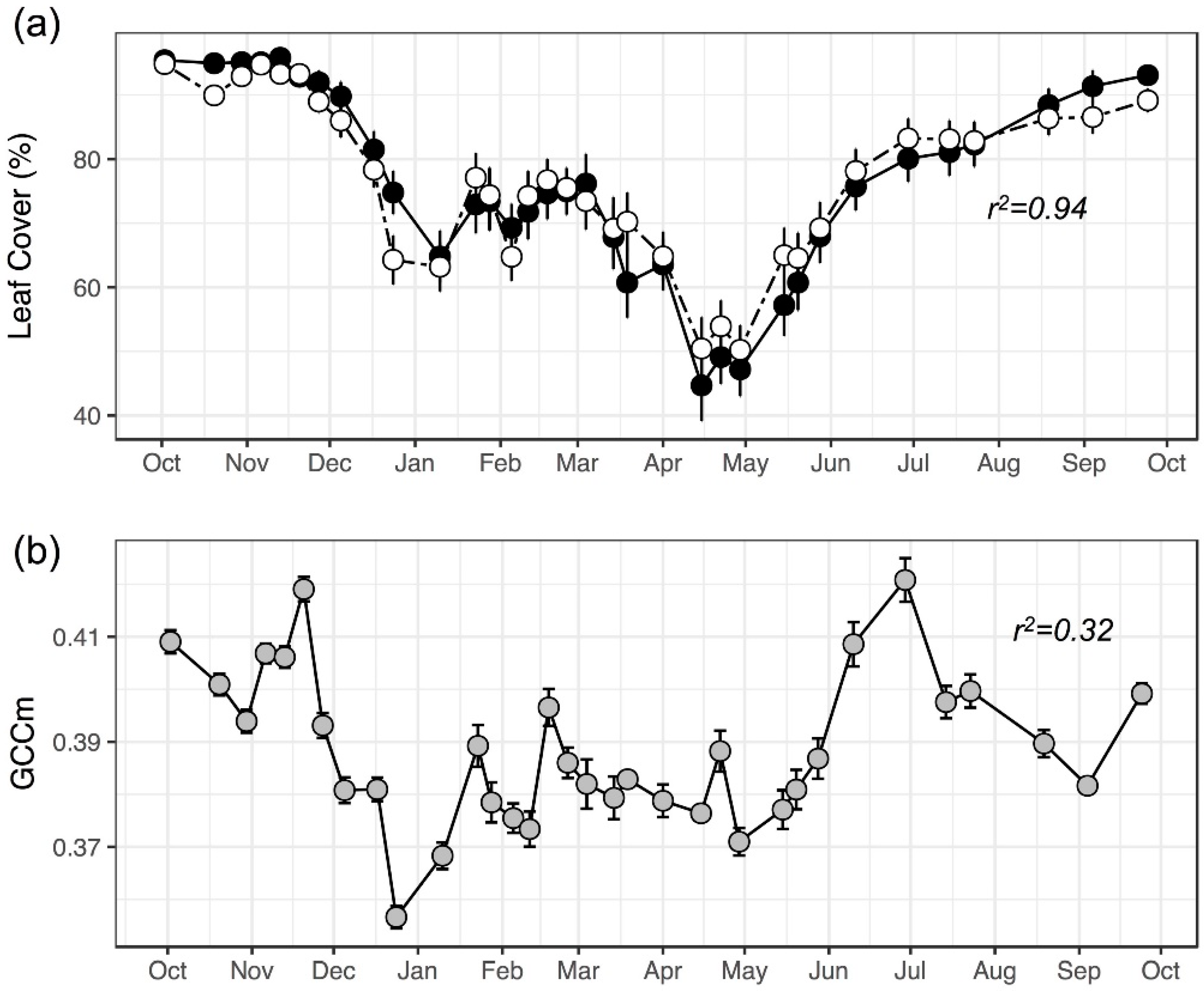
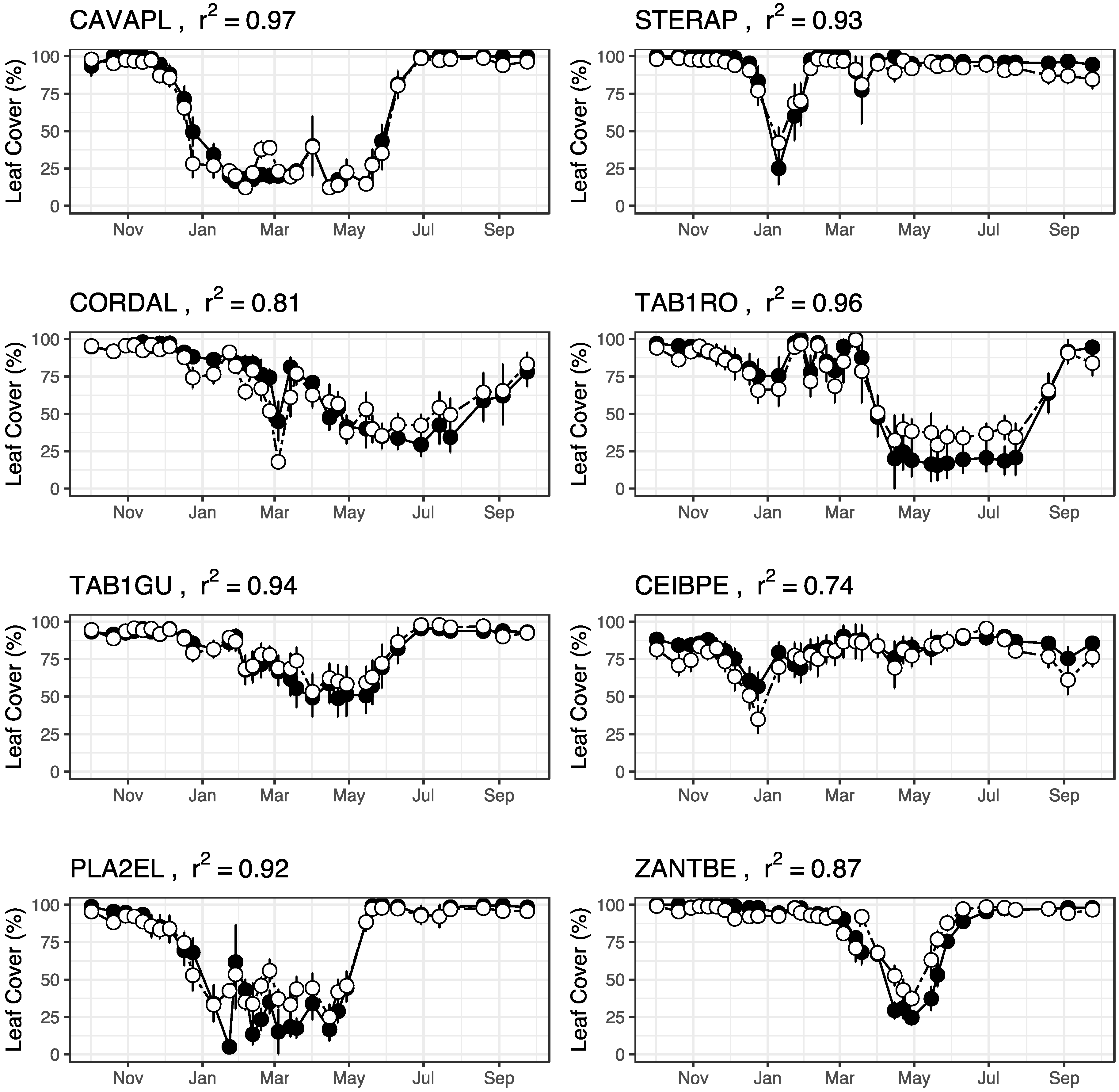
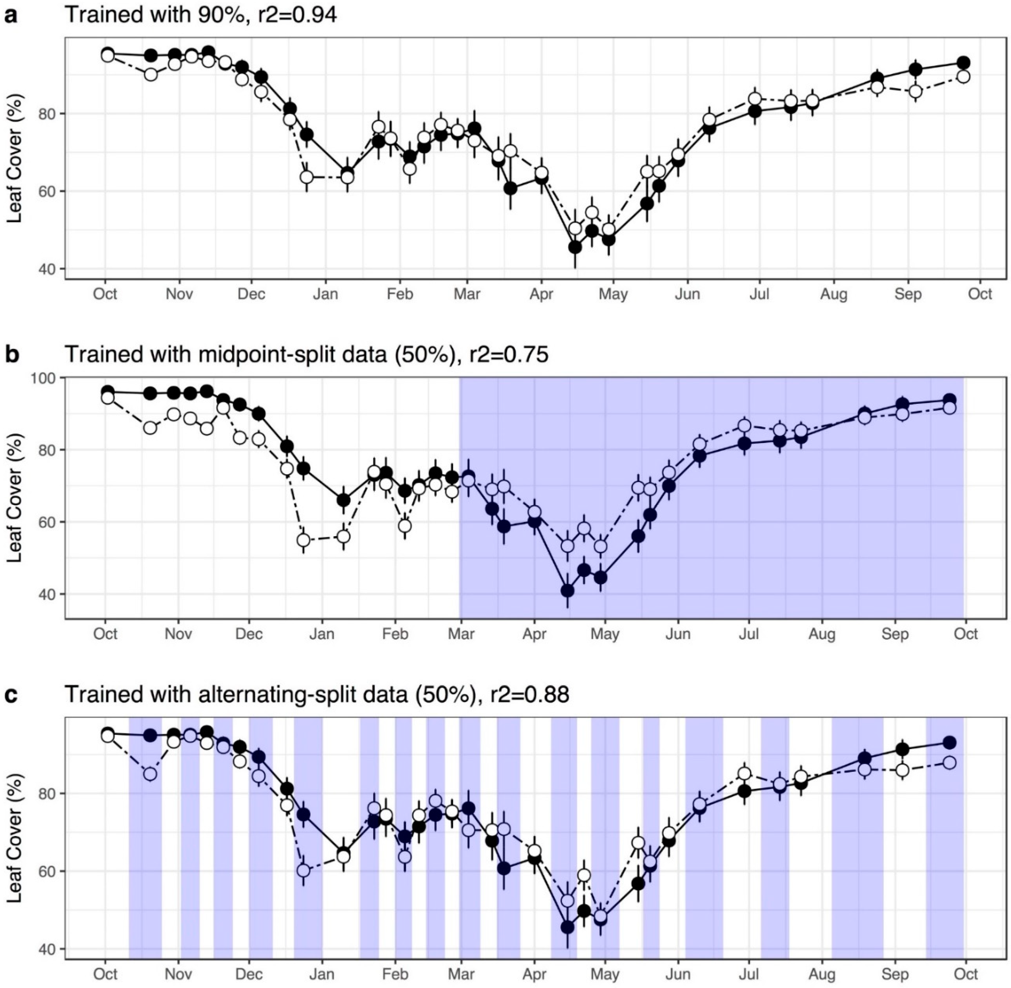
3.2. Model Performance in Capturing Intra-Annual Variation

Mean predicted leaf cover (averaged over all trees with observed leaf cover on a given date) closely tracked mean observed leaf cover over time (r² = 0.94 for 10-fold cross-validation; Figure 4a,

Table A3. Means and standard deviations (SD) of leaf cover on each sampling date for trees in the observation dataset.

UAV Flight Date	Mean Observed Leaf Cover	Mean Predicted Leaf Cover	SD Observed Leaf Cover	SD Predicted Leaf Cover	Difference in Means (Observed–Predicted)
10/02/14	95.52	94.78	12.23	9.33	0.74
10/20/14	95.05	90.21	9.39	13.48	4.84
10/30/14	95.22	92.83	8.88	12.44	2.39
11/06/14	95.14	94.96	9.56	8.20	0.18
11/13/14	95.84	93.61	9.51	9.49	2.23
11/20/14	93.04	93.43	14.52	11.72	−0.39
11/27/14	92.06	89.31	16.50	15.66	2.75
12/05/14	89.95	85.90	19.94	22.77	4.05
12/17/14	81.49	78.54	25.73	24.53	2.95
12/24/14	74.73	63.60	29.68	34.10	11.13
01/10/15	64.88	63.50	34.81	32.75	1.38
01/23/15	73.00	77.17	34.34	29.50	−4.17
01/28/15	73.75	74.40	34.07	31.87	−0.65
02/05/15	69.53	64.60	33.41	33.93	4.93
02/11/15	72.00	74.03	34.68	30.97	−2.03
02/18/15	74.73	76.72	32.19	25.97	−1.99
02/25/15	75.03	75.98	29.50	25.26	−0.95
03/04/15	75.16	72.59	31.21	29.65	2.57
03/14/15	67.84	68.40	32.93	32.49	−0.56
03/19/15	60.61	71.10	35.01	28.58	−10.49
04/01/15	64.11	65.53	32.57	30.48	−1.42
04/15/15	44.69	50.64	37.19	33.69	−5.95
04/22/15	49.23	54.28	36.60	35.00	−5.05
04/29/15	47.85	50.40	37.28	34.23	−2.55
05/15/15	57.29	65.90	38.68	33.88	−8.61
05/20/15	61.34	65.07	37.64	34.35	−3.73
05/28/15	68.35	69.76	36.65	35.50	−1.41
06/10/15	75.98	78.50	34.13	31.19	−2.52
06/29/15	80.28	83.85	33.25	27.83	−3.57
07/14/15	81.31	83.61	33.49	26.57	−2.30
07/23/15	82.42	83.32	30.90	27.10	−0.90
08/19/15	88.58	86.60	23.08	23.64	1.98
09/04/15	91.47	86.08	19.24	20.60	5.39
09/24/15	93.28	89.63	13.31	16.17	3.65

). In contrast, GCCm was only weakly correlated with mean observed leaf cover over time (r² = 0.32; Figure 4b). Predictions derived from using only the first half (2 October 2014 to 25 February 2015) or second half (4 March 2015 to 30 September 2015) of observations for model training did not perform as well as predictions from 10-fold cross-validation (Figure A2; r² = 0.75 for first-half/second-half split). In contrast, when alternate image dates were used for model training (i.e., every other sample date used for training, with the alternate dates used for validation), predictions performed nearly as well as those from 10-fold cross-validation (Figure A2; r² = 0.88 for alternating dates).

Intra-annual variation in species-level leaf cover (i.e., temporal variation in mean leaf cover of individuals of a given species) was well-predicted by the full model fit to other species, with mean (across species) r² of 0.89 (range 0.74 to 0.97), mean MAE of 6.0% (range 3.7% to 8.2%), and mean ME of 0.2% (range −4.6% to 4.3%) (Figure 5 and

Table A4. Goodness-of-fit statistics for out-of-sample species-level predictions (n = 34 dates). The model was trained on data for all trees except those belonging to the target (out-of-sample) species. Goodness-of-fit statistics were calculated by comparing mean predicted and observed leaf cover (averaged across individuals in the out-of-sample target species) for each sample date. r², MAE, and ME are as defined in Table A1.

Species	r2	MAE (%)	ME (%)
Cavanillesia platanifolia	0.97	4.58	−1.29
Ceiba pentandra	0.74	5.88	−4.61
Cordia alliodora	0.81	7.27	−1.77
Platypodium elegans	0.92	8.18	4.30
Sterculia apetala	0.93	4.22	−2.31
Handroanthus guayacan	0.94	3.71	2.61
Tabebuia rosea	0.96	7.86	2.40
Zanthoxylum ekmanii	0.87	6.16	2.52

; statistics are for out-of-sample species-level predictions).

Intra-annual variation in individual-tree leaf cover was well-predicted by the full model fit to other individuals, with mean (across individuals) r² of 0.82 (range 0.36 to 0.99), mean MAE of 8.1% (range 1.2% to 17.9%), and ME of −0.07% (range −12.5% to 12.7%) (Figure 6;

Table A5. Goodness-of-fit statistics for out-of-sample individual tree-level predictions (n = 34 dates). The model was trained on data for all trees excluding the target (out-of-sample) tree. Goodness-of-fit statistics were calculated by comparing predicted and observed leaf cover for each tree on each sample date. Goodness-of-fit statistics were then pooled across individuals within each species to calculate the means and standard deviations (SD) reported in the table. r², MAE, and ME are as defined in Table A1.

Species	Mean r 2 (SD)	Mean MAE (SD)	Mean ME (SD)
Cavanillesia platanifolia	0.92 (0.09)	6.69 (2.47)	−1.86 (4.08)
Ceiba pentandra	0.73 (0.12)	9.24 (3.50)	−3.57 (4.33)
Cordia alliodora	0.64 (0.15)	11.95 (3.00)	−0.81 (6.77)
Platypodium elegans	0.87 (0.08)	8.09 (3.91)	1.39 (6.28)
Sterculia apetala	0.87 (0.17)	4.36 (2.25)	−1.90 (1.97)
Handroanthus guayacan	0.84 (0.08)	7.83 (3.54)	2.44 (5.58)
Tabebuia rosea	0.89 (0.07)	10.60 (2.64)	2.11 (4.64)
Zanthoxylum ekmanii	0.76 (0.12)	7.70 (2.01)	2.06 (3.61)

; statistics are for out-of-sample individual-level predictions). MAE for intra-annual variation tended to decrease across individual trees with increasing mean annual leaf cover, but r² was not significantly correlated with mean annual leaf cover (Figure A3). Neither MAE nor r² for intra-annual variation was significantly correlated with crown size (Figure A3). Of the 15 crowns with r² ≤ 0.70, 13 belonged to Cordia alliodora and Ceiba pentandra (Figure 6h).

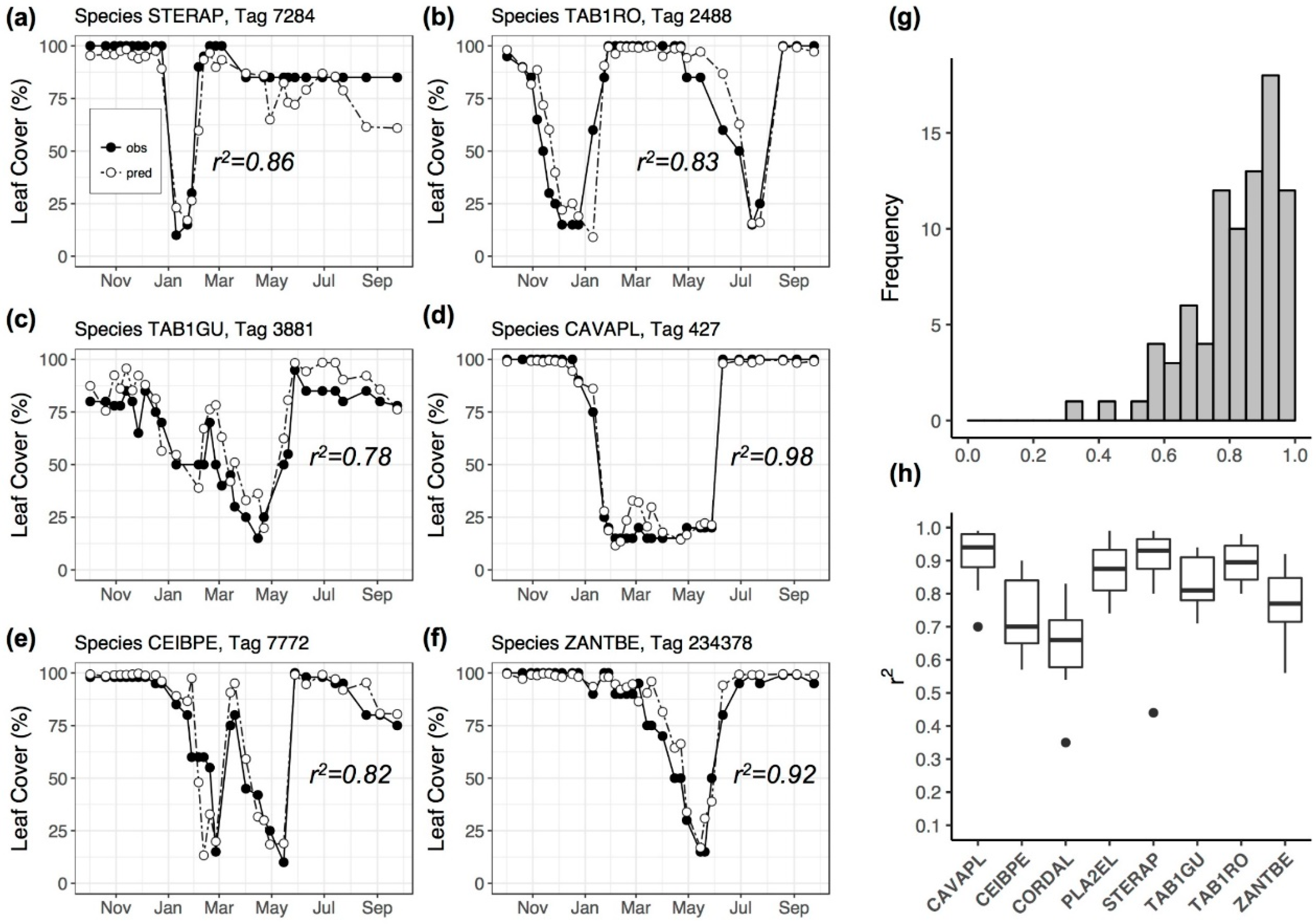
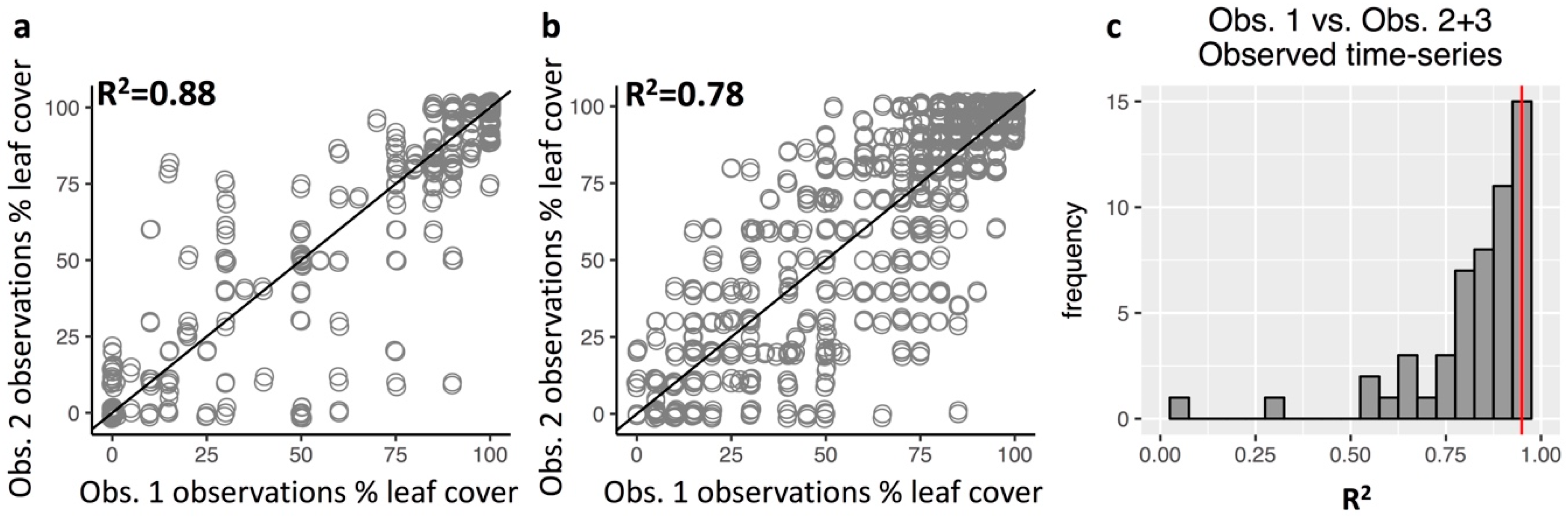
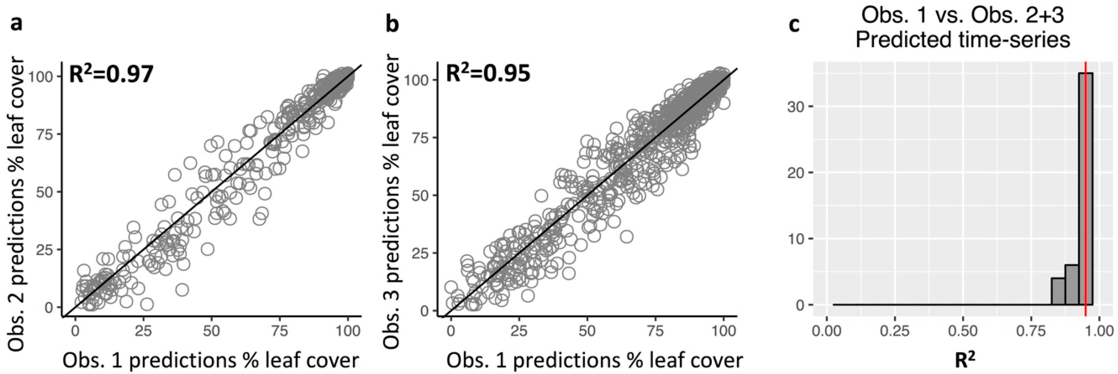
3.3. Repeatability of Visual Leaf-Cover Estimates and Model Predictions

Estimates of percent leaf cover based on visual interpretation of images were largely repeatable among multiple observers (r² = 0.88 and 0.78 for comparisons between pairs of human observers; Figure A4). Model predictions of leaf cover for individual images were insensitive to observer differences (r² = 0.97 and 0.95 for comparisons between pairs of predictions derived from different observers’ estimates; Figure A5a–b). Model predictions of leaf cover time-series for individual trees were also insensitive to observer differences (Figure A5c).

4. Discussion

Our framework for analyzing UAV images to quantify individual-level tree phenology in a tropical forest—combining field work, visual image interpretation, and a machine learning algorithm—performed well at predicting leaf cover of individual crowns on a given date and quantifying intra-annual patterns of leaf phenology for individuals and species. The best-performing model used all 14 image features that we explored, including means and standard deviations of color channels, as well as more computationally intensive features (end members from a mixture model and a moving-window measure of pixel variability). A model using only color means and standard deviations performed nearly as well as the full model. A model based only on the mean of the green color channel, which has been widely used in phenological studies of temperate ecosystems, performed poorly at our tropical forest site. We suggest that texture features, which quantify variability within images, should be considered in future studies of canopy phenology, particularly in cases where mean color features do not perform well. Some texture features may be more robust than widely-used mean color features to highly variable illumination within and among sampling dates and imperfect image calibration (as in our study).

4.1. Image Features for Quantifying Phenology

Image texture features, particularly the standard deviation of the individual color channels (Bsd, Gsd and Rsd), were useful for quantifying leaf cover phenology in this tropical forest. Texture features capture variability in brightness and color, which is higher in leafless and partially leafless crowns due to exposed branches and shadows. Texture features were only weakly correlated with color features (Table A2), indicating that these two feature classes provide largely independent information. Texture features may be particularly useful when illumination is variable among images (as in our dataset), because much of the variability in color will be preserved even if overall illumination changes. The single most predictive image feature we tested was the standard deviation in blue color (Bsd; Table 3 and Table A1). The blue channel is a chlorophyll absorption band, such that leaves and shadows appear dark and branches appear light. Therefore, within-crown variability in the blue channel increases as leaves are dropped, branches are exposed, and within-crown shadowing increases (Figure A6). Although the red channel also includes wavelengths with high chlorophyll absorption, standard deviation in red color (Rsd) did not perform as well as standard deviation in blue color (Bsd).

The most commonly used image metric in studies of leaf phenology in temperate forests—mean GCC (GCCm)—had limited power to explain variation in leaf cover among crowns in our study, and color metrics were less useful than texture metrics in general. Multiple factors may have contributed to the limited ability of color metrics to predict leaf cover in our dataset. First, tropical forests have multi-layered canopies [33], and understory trees are less likely to be deciduous than canopy trees [40], such that an image from above a crown that is partially or fully deciduous often includes considerable green from understory trees. Second, our study site has high canopy tree species diversity, and leaf color can vary considerably within and among species with leaf traits and leaf age [41,42]. We can gain insight into the usefulness of different image features by considering only those tree crowns with 100% leaf cover on a given date. For these fully-leaved crowns, a robust image feature (e.g., one that is insensitive to variation in illumination due to sun angle and cloud cover) should be relatively constant throughout the year. For fully-leaved crowns, GCCm was highly variable over time, whereas the standard deviation of the blue color channel (Bsd) was more constant (Figure A7). This comparison helps explain why Bsd was a better predictor for leaf cover than GCCm in our analysis.

In general, the ability of color versus texture metrics to predict leaf cover (or other ecological features of a tree crown) will depend strongly on characteristics of the images, as well as on the study site. Higher pixel resolution will provide more pixels per tree crown, likely increasing the observable differences in texture. With lower pixel resolution, mean crown color may provide more information than texture. Similarly, blurry images will decrease the color variability among pixels, and make texture measures less useful in comparison to mean color metrics. In contrast, more consistent illumination or better color normalization across dates will increase the utility of color metrics, as will similarity in leaf color across species and crowns within a dataset. Finally, our study focused on leaf cover, which is only one aspect of canopy phenology. Mean color metrics may be useful for quantifying other aspects of canopy phenology [15]; e.g., photosynthetic capacity depends not only on leaf cover, but also on leaf quality, which may be correlated with mean color metrics related to chlorophyll absorption bands (e.g., red and blue channels).

4.2. Sources of Prediction Error

Any errors in the human interpretation of the images would of course limit the extent to which such observations represent true leaf cover. However, observation errors are likely to be less common for our observations than for standard ground-based observations of leaf cover. The UAV images we analyzed provide an unobstructed view of the canopy from above (Figure 3), allowing for much easier human interpretation compared to observers on the ground looking up at the canopy (sometimes over 40 m tall) through what is often a dense, multi-layered understory. In our study, leaf cover estimates from visual interpretation of images by different observers were largely repeatable despite the lack of observer training (Figure A4), and model predictions were insensitive to modest differences among different observers (Figure A5 and

Table A6. Comparison of models trained with different sets of observations: ‘Observer 1 full’ refers to the full set of observations used to obtain the Main text model Results (2422 images belonging to 85 individual crowns); ‘Observer 1 subset’ is the subset of the full dataset (1780 images belonging to 58 individual crowns) corresponding to the same 58 crowns for which Observer 2 or 3 observations were available; ‘Observer 2+3 subset’ refers to observations from either Observer 2 or Observer 3 (1747 images belonging to 58 individual crowns for the combined Observer 2+3 dataset). Values in the columns for each observer dataset report the r² (squared Pearson correlation) between observations and out-of-sample predictions from 10-fold cross-validation.

Model Description	# of Features	Obs. 1 Full	Obs. 1 Subset	Obs. 2+3 Subset
Mean Green Chromatic Coordinate	1	0.52	0.43	0.38
Means of Green, Blue, and Red Chromatic Coordinates	3	0.62	0.55	0.49
All mean color features	6	0.68	0.64	0.55
Standard deviation of green channel	1	0.25	0.19	0.15
Standard deviation of blue channel	1	0.63	0.56	0.48
Standard deviations of all color features	6	0.71	0.64	0.54
GLCM correlations	2	0.39	0.31	0.25
All texture measures including standard deviations of color features and GLCM correlation	8	0.75	0.69	0.59
Mean Green Chromatic Coordinate and standard deviation of green channel	2	0.66	0.61	0.53
Mean Chromatic Coordinates and standard deviations of color channels	6	0.78	0.74	0.65
Full model	14	0.84	0.80	0.72

).

Beyond observation errors, the amount and characteristics of training data (e.g., the range of image features covered in the training dataset) could strongly affect model performance. In our study, model performance was more sensitive to the seasonal distribution of training data than the amount of training data. Specifically, if only half of the observations were used for training, the model still performed well if the observations were distributed throughout the entire year (Figure A2c), whereas model performance was worse if training data included only the first half (or only the second half) of the observation time-series (Figure 6b). It is likely that the temporal distribution of training data is important because sun angle, cloud cover, atmospheric smoke and haze, or other image features changed over the one-year period of sampling, so that temporally-restricted training data do not include the full “image space” needed for robust predictions. This “image space” issue may also explain why out-of-sample predictions were relatively poor for some species and individuals (Figure 5 and Figure 6), e.g., if certain species or individuals have image features that were not well-represented in the training data. Future community-level analyses that target additional species (beyond the eight species studied here) may therefore benefit from additional training data.

4.3. Advances in Phenological Observations of Tropical Forests

Our UAV-based methods precisely document intra-annual leaf cover changes in many individual canopy trees at fine temporal resolution, and thereby precisely quantify interspecific and intraspecific variation in deciduousness within a tropical forest. These methods provide considerably more detailed information on leaf phenology than was previously available, even in this exceptionally well-studied tropical site. Previous studies of leaf phenology at this site involved qualitative descriptions of species leafing patterns [4], field observations of a few individuals of selected species at a few dates during the dry season [6], and analysis of litterfall patterns [11,43]. Litterfall data are perhaps the most widely available type of leaf phenology data, yet they are usually collected only at the stand scale, and do not in and of themselves provide information on whether (or when) trees are deciduous because they provide no information on the timing of leaf production. No previous study at this tropical forest site provided comprehensive, quantitative information on intra-annual leaf cover changes within and among species. As discussed below, the methods we present here could be extended to quantify phenology of additional species at our study site (based on currently available imagery), as well as at other sites (if imagery is available).

Our results document subtle patterns, including the speed of leaf cover change and the degree of intraspecific variation in leaf phenology, and their variation among species. Some species (Cavanillesia platanifolia, Zanthoxylum ekmanii) show rapid declines in leaf cover, while other species (Cordia alliodora, Handroanthus guayacan) show more gradual declines. Some species (Cavanillesia platanifolia, Sterculia apetala, and Zanthoxylum ekmanii) exhibit highly synchronous leaf cover variation, while other species (Platypodium elegans, Cavanillesia platanifolia, Cordia alliodora) show a high level of intraspecific variation in leaf phenology (Figure A8). Some individuals of some species showed two periods of low leaf cover during the year, which had been previously documented for Tabebuia rosea [4] (Figure 5), but not for Ceiba pentandra (Figure 5 and Figure 6e) or Platypodium elegans. The leaf cover patterns illustrated in this study can be further analyzed to estimate phenology metrics such as dates and rates of leaf cover increase and decrease. Variability among species and individuals in the timing, degree, and number of deciduous events per year makes defining and quantifying these phenology metrics complicated in tropical forests. This topic is beyond the scope of this paper and will be addressed in a future study.

The methods described in this paper could be used to document the phenology of many individual canopy plants over long time periods. Although our analyses here focused on only 85 crowns, our imagery includes time series for over 1600 delineated crowns, illustrating the potential for large-scale monitoring with these methods. Our analyses demonstrate that UAV images, including images collected under cloudy conditions and with variable illumination, can provide high-resolution and high-quality quantitative data on leaf cover, which should allow for long-term observations of large numbers of individuals and species. Long-term observations in tropical forests have been highlighted as a critical need for understanding drivers of phenology [2]. Given the recent advances in the reliability of UAVs, our methods could be easily applied at other sites and over larger areas. Other forest dynamics plots, where canopy trees have already been mapped and identified to species [44] would be obvious candidate sites to apply our methods. Even in areas where trees have not been mapped and identified on the ground, our methods could still be used to quantify canopy phenology at the stand scale and for individual crowns (even without data on species identity). Our methods performed well throughout both the dry and wet seasons (Figure 4a), suggesting they would work well in longer-term studies.

Quantitative information on inter- and intraspecific variation in canopy phenology constitutes a valuable resource for understanding the environmental drivers of tropical tree phenology and thereby for improving models of forest carbon and water fluxes. Recent studies demonstrate that stand-level leaf phenology is the primary driver of photosynthetic phenology in Amazon forests [14], and that mechanistic models of leaf phenology incorporating interspecific variation can improve predictions of stand-level leaf phenology [45]. High-resolution, UAV-derived phenology data for multiple species and plant functional types could be used to calibrate or drive ecosystem process models, enabling improved predictions of tropical forest ecosystem function across time and space.

5. Conclusions

The methodology presented here, tested with eight canopy tree species, could be applied to monitor phenology of individuals and species at the landscape scale (e.g., 1000s of trees) in tropical forests. Machine learning algorithms are becoming widely used to translate image data, including images from UAVs, into ecological information. Our study demonstrates three key components of a research program that combines UAV images and machine learning to quantify tropical forest phenology. The first key component is fieldwork that links tree crowns in UAV images to trees that are monitored on the ground (i.e., in forest inventory plots), thus allowing identification of species, as well as linkages to other data not used in the present study (e.g., growth rates and functional traits of individual trees). Although much of the methodology we present could be applied to monitor stand-level phenology in landscapes where ground data are not available, the link between UAV images (or other fine-spatial-resolution remote-sensing data) and ground data is critical for monitoring phenology at the species level. The second key component in our pipeline is generating training data for machine learning algorithms using visual estimates of leaf cover, which were largely repeatable among different human observers. UAV images provide a clear, unobstructed view of the canopy, which likely makes visual estimation of leaf cover less error-prone compared to traditional ground-based phenological studies in dense, multi-layered tropical forests. The third key component is including information on color variation (“texture”) in image analysis. Models that included both color and texture features had better predictive ability than those based only on color features. We suspect that texture features are less sensitive than color features to variation in illumination within and among dates, and to imperfect image calibration. Our analysis of eight species showed contrasting patterns, with some species having nearly synchronous phenology among individuals, and other species having high levels of intraspecific variation. Landscape-scale applications of our methodology will allow for unprecedented community-level analyses of intra- and interspecific variation in tropical forest canopy phenology.

References

1. Pachauri, R.K.; Allen, M.R.; Barros, V.R.; Broome, J.; Cramer, W.; Christ, R.; Church, J.A.; Clarke, L.; Dahe, Q.; Dasgupta, P.; et al. Climate Change 2014: Synthesis Report. Contribution of Working Groups I, II and III to the Fifth Assessment Report of the Intergovernmental Panel on Climate Change; Pachauri, R.K., Meyer, L., Eds.; IPCC: Geneva, Switzerland, 2014. [Google Scholar]
2. Richardson, A.D.; Keenan, T.F.; Migliavacca, M.; Ryu, Y.; Sonnentag, O.; Toomey, M. Climate change, phenology, and phenological control of vegetation feedbacks to the climate system. Agric. For. Meteorol. 2013, 169, 156–173. [Google Scholar] [CrossRef]
3. Wolkovich, E.M.; Cook, B.I.; Davies, T.J. Progress towards an interdisciplinary science of plant phenology: Building predictions across space, time and species diversity. New Phytol. 2014, 201, 1156–1162. [Google Scholar] [CrossRef] [PubMed]
4. Croat, T.B. Flora of Barro Colorado Island; Stanford University Press: Palo Alto, CA, USA, 1978; ISBN 978-0-8047-0950-7. [Google Scholar]
5. Leigh, E.G. Tropical Forest Ecology: A View from Barro Colorado Island; Oxford University Press: Oxford, UK, 1999; ISBN 978-0-19-509603-3. [Google Scholar]
6. Condit, R.; Watts, K.; Bohlman, S.A.; Pérez, R.; Foster, R.B.; Hubbell, S.P. Quantifying the deciduousness of tropical forest canopies under varying climates. J. Veg. Sci. 2000, 11, 649–658. [Google Scholar] [CrossRef] [Green Version]
7. Reich, P.B.; Uhl, C.; Walters, M.B.; Prugh, L.; Ellsworth, D.S. Leaf demography and phenology in Amazonian rain forest: A census of 40,000 leaves of 23 tree species. Ecol. Monogr. 2004, 74, 3–23. [Google Scholar] [CrossRef]
8. Elliott, S.; Baker, P.J.; Borchert, R. Leaf flushing during the dry season: The paradox of Asian monsoon forests. Glob. Ecol. Biogeogr. 2006, 15, 248–257. [Google Scholar] [CrossRef]
9. Williams, L.J.; Bunyavejchewin, S.; Baker, P.J. Deciduousness in a seasonal tropical forest in western Thailand: Interannual and intraspecific variation in timing, duration and environmental cues. Oecologia 2008, 155, 571–582. [Google Scholar] [CrossRef] [PubMed]
10. Wright, S.J.; Cornejo, F.H. Seasonal drought and leaf fall in a tropical forest. Ecology 1990, 71, 1165–1175. [Google Scholar] [CrossRef]
11. Detto, M.; Wright, S.J.; Calderón, O.; Muller-Landau, H.C. Resource acquisition and reproductive strategies of tropical forest in response to the El Niño–Southern Oscillation. Nat. Commun. 2018, 9, 913. [Google Scholar] [CrossRef]
12. Samanta, A.; Ganguly, S.; Vermote, E.; Nemani, R.R.; Myneni, R.B. Why is remote sensing of Amazon forest greenness so challenging? Earth Interact. 2012, 16, 1–14. [Google Scholar] [CrossRef]
13. Morton, D.C.; Nagol, J.; Carabajal, C.C.; Rosette, J.; Palace, M.; Cook, B.D.; Vermote, E.F.; Harding, D.J.; North, P.R.J. Amazon forests maintain consistent canopy structure and greenness during the dry season. Nature 2014, 506, 221–224. [Google Scholar] [CrossRef]
14. Wu, J.; Albert, L.P.; Lopes, A.P.; Restrepo-Coupe, N.; Hayek, M.; Wiedemann, K.T.; Guan, K.; Stark, S.C.; Christoffersen, B.; Prohaska, N.; et al. Leaf development and demography explain photosynthetic seasonality in Amazon evergreen forests. Science 2016, 351, 972–976. [Google Scholar] [CrossRef] [PubMed] [Green Version]
15. Lopes, A.P.; Nelson, B.W.; Wu, J.; de Alencastro Graça, P.M.L.; Tavares, J.V.; Prohaska, N.; Martins, G.A.; Saleska, S.R. Leaf flush drives dry season green-up of the Central Amazon. Remote Sens. Environ. 2016, 182, 90–98. [Google Scholar] [CrossRef]
16. Saleska, S.R.; Wu, J.; Guan, K.; Araujo, A.C.; Huete, A.; Nobre, A.D.; Restrepo-Coupe, N. Dry-season greening of Amazon forests. Nature 2016, 531, E4–E5. [Google Scholar] [CrossRef] [PubMed]
17. Sánchez-Azofeifa, A.; Rivard, B.; Wright, J.; Feng, J.-L.; Li, P.; Chong, M.M.; Bohlman, S.A. Estimation of the distribution of Tabebuia guayacan (Bignoniaceae) using high-resolution remote sensing imagery. Sensors 2011, 11, 3831–3851. [Google Scholar] [CrossRef] [PubMed]
18. Kellner, J.R.; Hubbell, S.P. Adult mortality in a low-density tree population using high-resolution remote sensing. Ecology 2017, 98, 1700–1709. [Google Scholar] [CrossRef] [PubMed]
19. Alberton, B.; Almeida, J.; Helm, R.; Torres, R.D.S.; Menzel, A.; Morellato, L.P.C. Using phenological cameras to track the green up in a cerrado savanna and its on-the-ground validation. Ecol. Inform. 2014, 19, 62–70. [Google Scholar] [CrossRef]
20. Klosterman, S.; Richardson, A.D. Observing spring and fall phenology in a deciduous forest with aerial drone imagery. Sensors 2017, 17, 2852. [Google Scholar] [CrossRef]
21. Klosterman, S. Fine-scale perspectives on landscape phenology from unmanned aerial vehicle (UAV) photography. Agric. For. Meteorol. 2018, 248, 397–407. [Google Scholar] [CrossRef]
22. Srinivasan, G.; Shobha, G. Statistical texture analysis. Proc. World Acad. Sci. Eng. Technol. 2008, 36, 1264–1269. [Google Scholar]
23. Culbert, P.D.; Radeloff, V.C.; St-Louis, V.; Flather, C.H.; Rittenhouse, C.D.; Albright, T.P.; Pidgeon, A.M. Modeling broad-scale patterns of avian species richness across the Midwestern United States with measures of satellite image texture. Remote Sens. Environ. 2012, 118, 140–150. [Google Scholar] [CrossRef] [Green Version]
24. Tuanmu, M.-N.; Jetz, W. A global, remote sensing-based characterization of terrestrial habitat heterogeneity for biodiversity and ecosystem modelling. Glob. Ecol. Biogeogr. 2015, 24, 1329–1339. [Google Scholar] [CrossRef]
25. Hofmann, S.; Everaars, J.; Schweiger, O.; Frenzel, M.; Bannehr, L.; Cord, A.F. Modelling patterns of pollinator species richness and diversity using satellite image texture. PLoS ONE 2017, 12, e0185591. [Google Scholar] [CrossRef] [PubMed]
26. Freeman, E.A.; Moisen, G.G.; Coulston, J.W.; Wilson, B.T. Random forests and stochastic gradient boosting for predicting tree canopy cover: Comparing tuning processes and model performance. Can. J. For. Res. 2015, 46, 323–339. [Google Scholar] [CrossRef]
27. Ahmed, O.S.; Franklin, S.E.; Wulder, M.A.; White, J.C. Characterizing stand-level forest canopy cover and height using Landsat time series, samples of airborne LiDAR, and the Random Forest algorithm. ISPRS J. Photogramm. Remote Sens. 2015, 101, 89–101. [Google Scholar] [CrossRef]
28. Hubbell, S.P.; Foster, R.B.; O’Brien, S.T.; Harms, K.E.; Condit, R.; Wechsler, B.; Wright, S.J.; De Lao, S.L. Light-gap disturbances, recruitment limitation, and tree diversity in a neotropical forest. Science 1999, 283, 554–557. [Google Scholar] [CrossRef] [PubMed]
29. Paton, S. Meteorological and Hydrological Summary for Barro Colorado Island; Smithsonian Tropical Research Institute: Balboa, Panama, 2017. [Google Scholar]
30. Dandois, J.P.; Olano, M.; Ellis, E.C. Optimal Altitude, overlap, and weather conditions for computer vision UAV estimates of forest structure. Remote Sens. 2015, 7, 13895–13920. [Google Scholar] [CrossRef]
31. Zahawi, R.A.; Dandois, J.P.; Holl, K.D.; Nadwodny, D.; Reid, J.L.; Ellis, E.C. Using lightweight unmanned aerial vehicles to monitor tropical forest recovery. Biol. Conserv. 2015, 186, 287–295. [Google Scholar] [CrossRef] [Green Version]
32. Lobo, E.; Dalling, J.W. Effects of topography, soil type and forest age on the frequency and size distribution of canopy gap disturbances in a tropical forest. Biogeosciences 2013, 10, 6769–6781. [Google Scholar] [CrossRef] [Green Version]
33. Bohlman, S.; Pacala, S. A forest structure model that determines crown layers and partitions growth and mortality rates for landscape-scale applications of tropical forests. J. Ecol. 2012, 100, 508–518. [Google Scholar] [CrossRef]
34. Graves, S.; Gearhart, J.; Caughlin, T.T.; Bohlman, S. A digital mapping method for linking high-resolution remote sensing images to individual tree crowns. PeerJ Prepr. 2018, 6, e27182v1. [Google Scholar]
35. Richardson, A.D.; Braswell, B.H.; Hollinger, D.Y.; Jenkins, J.P.; Ollinger, S.V. Near-surface remote sensing of spatial and temporal variation in canopy phenology. Ecol. Appl. 2009, 19, 1417–1428. [Google Scholar] [CrossRef] [PubMed]
36. Adams, J.B.; Sabol, D.E.; Kapos, V.; Almeida Filho, R.; Roberts, D.A.; Smith, M.O.; Gillespie, A.R. Classification of multispectral images based on fractions of endmembers: Application to land-cover change in the Brazilian Amazon. Remote Sens. Environ. 1995, 52, 137–154. [Google Scholar] [CrossRef]
37. Haralick, R.M.; Shanmugam, K. Textural features for image classification. IEEE Trans. Syst. Man Cybern. 1973, 6, 610–621. [Google Scholar] [CrossRef]
38. Friedman, J.H. Stochastic gradient boosting. Comput. Stat. Data Anal. 2002, 38, 367–378. [Google Scholar] [CrossRef]
39. Hastie, T.; Tibshirani, R.; Friedman, J. The Elements of Statistical Learning: Data Mining, Inference, and Prediction, 2nd ed.; Springer Series in Statistics; Springer: New York, NY, USA, 2009; ISBN 978-0-387-84857-0. [Google Scholar]
40. Frankie, G.W.; Baker, H.G.; Opler, P.A. Comparative phenological studies of trees in tropical wet and dry forests in the lowlands of Costa Rica. J. Ecol. 1974, 62, 881–919. [Google Scholar] [CrossRef]
41. Asner, G.P. Biophysical and biochemical sources of variability in canopy reflectance. Remote Sens. Environ. 1998, 64, 234–253. [Google Scholar] [CrossRef]
42. Wu, J.; Chavana-Bryant, C.; Prohaska, N.; Serbin, S.P.; Guan, K.; Albert, L.P.; Yang, X.; van Leeuwen, W.J.D.; Garnello, A.J.; Martins, G.; et al. Convergence in relationships between leaf traits, spectra and age across diverse canopy environments and two contrasting tropical forests. New Phytol. 2017, 214, 1033–1048. [Google Scholar] [CrossRef]
43. Wieder, R.K.; Wright, S.J. Tropical forest litter dynamics and dry season irrigation on Barro Colorado Island, Panama. Ecology 1995, 76, 1971–1979. [Google Scholar] [CrossRef]
44. Anderson-Teixeira, K.J.; Davies, S.J.; Bennett, A.C.; Gonzalez-Akre, E.B.; Muller-Landau, H.C.; Wright, S.J.; Abu Salim, K.; Almeyda Zambrano, A.M.; Alonso, A.; Baltzer, J.L.; et al. CTFS-ForestGEO: A worldwide network monitoring forests in an era of global change. Glob. Chang. Biol. 2015, 21, 528–549. [Google Scholar] [CrossRef]
45. Xu, X.; Medvigy, D.; Powers, J.S.; Becknell, J.M.; Guan, K. Diversity in plant hydraulic traits explains seasonal and inter-annual variations of vegetation dynamics in seasonally dry tropical forests. New Phytol. 2016, 212, 80–95. [Google Scholar] [CrossRef]
46. Du, Y.; Teillet, P.M.; Cihlar, J. Radiometric normalization of multitemporal high-resolution satellite images with quality control for land cover change detection. Remote Sens. Environ. 2002, 82, 123–134. [Google Scholar] [CrossRef]
47. Adams, J.B.; Gillespie, A.R. Remote Sensing of Landscapes with Spectral Images; Cambridge University Press: Cambridge, UK, 2006; ISBN 978-0-521-66221-5. [Google Scholar]
48. Grizonnet, M.; Michel, J.; Poughon, V.; Inglada, J.; Savinaud, M.; Cresson, R. Orfeo ToolBox: Open source processing of remote sensing images. Open Geospat. Data Softw. Stand. 2017, 2, 15. [Google Scholar] [CrossRef]
49. Jordahl, K. GeoPandas: Python Tools for Geographic Data. Available online: https://github. com/geopandas/geopandas (accessed on 15 May 2019).
50. Ridgeway, G. GBM: Generalized boosted regression models. R Package Version 2006, 1, 55. [Google Scholar]
51. Ridgeway, G. Generalized Boosted Models: A guide to the gbm package. Update 2007, 1, 2007. [Google Scholar]
Figure 1. Schematic workflow for predicting leaf phenology patterns of individual crowns from UAV (Unmanned aerial vehicles) images. See Materials and Methods for details.
Remotesensing 11 01534 g001
Figure 2. UAV orthomosaic of the entire 50-ha plot (red rectangle). The orthomosaic is from 2 October 2014. A subset of the UAV image (orange square) with delineated tree crowns is shown on the right.
Remotesensing 11 01534 g002
Figure 3. Example of tree image time-series in the UAV dataset. Selected images from the time series for a single crown (Ceiba pentandra, tag 4092). The text box in each image gives the date (MM-DD-YY) and the observed/predicted (full model) leaf cover. 24 out of 34 dates are shown; the 10 excluded dates have observed and predicted leaf cover near 100%.
Remotesensing 11 01534 g003
Figure 4. (a) Predicted and observed mean leaf cover (average across all crowns on a given date) and (b) mean Green Chromatic Coordinate (GCCm). (a) Observed leaf cover (filled circles, solid line) and leaf cover predicted by the full model (open circles, dashed line). The r2 values are the squared Pearson correlation over time between (a) mean observed and predicted leaf cover, and (b) mean observed leaf cover and mean GCCm. Values do not represent stand-level means, because our analysis targeted deciduous species that are a non-random subset of the mixed evergreen/deciduous forest community. The number of crowns ranges from 40 to 85 per date (some crowns were excluded on a given date based on filtering criteria described in Materials and Methods). Vertical bars are standard errors.
Remotesensing 11 01534 g004
Figure 5. Evaluation of model performance for out-of-sample species predictions. Observed (filled circles and solid lines) and predicted (open circles and dashed lines) time series for species-level means. Predictions are from the full model trained with a dataset that excluded the target (out-of-sample) species. r2 is the squared Pearson correlation over time between observed and predicted species means. Additional goodness-of-fit metrics are in Table A4. Species abbreviations are defined in Table 1.
Remotesensing 11 01534 g005
Figure 6. Evaluation of model performance for out-of-sample individual predictions. (af) Observed (filled circles, solid lines) and predicted (open circles, dashed lines) time series for selected individual trees; r2 is the squared Pearson correlation over time between observed and predicted leaf cover. (g) Distribution of r2 values across all trees (85) in the observation dataset (mean r2 = 0.83; SD = 0.13). (h) Distribution of r2 values for each species in the observation dataset. Predictions are from the full model trained with a dataset that excluded the target (out-of-sample) individual. Additional goodness-of-fit metrics are in Table A5. Species abbreviations are defined in Table 1.
Remotesensing 11 01534 g006