The Integration of Multi-source Remotely-Sensed Data in Support of the Classification of Wetlands

Department of Earth and Space Science and Engineering, York University, 4700 Keele st., Toronto, ON M3J1P3, Canada
*
Author to whom correspondence should be addressed.
Remote Sens. 2019, 11(13), 1537; https://0-doi-org.brum.beds.ac.uk/10.3390/rs11131537
Submission received: 19 May 2019
/
Revised: 24 June 2019
/
Accepted: 26 June 2019
/
Published: 28 June 2019
(This article belongs to the Special Issue Innovative Remote Sensing for Monitoring and Assessment of Natural Resources)
Abstract
:Wetlands play a key role in regional and global environments, and are critically linked to major issues such as climate change, wildlife habitat, biodiversity, water quality protection, and global carbon and methane cycles. Remotely-sensed imagery provides a means to detect and monitor wetlands on large scales and with regular frequency. In this project, methodologies were developed to classify wetlands (Open Bog, Treed Bog, Open Fen, Treed Fen, and Swamps) from multi-source remotely sensed data using advanced classification algorithms. The data utilized included multispectral optical and thermal data (Landsat-5) and Radar imagery from RADARSAT-2 and Sentinel-1. The goals were to determine the best way to combine the aforementioned imagery to classify wetlands, and determine the most significant image features. Classification algorithms investigated in this study were Naive Bayes, K-Nearest Neighbor (K-NN), Support Vector Machine (SVM), and Random Forest (RF). Based on the test results in the study area in Northern Ontario, Canada (49°31′.34N, 80°43′37.04W), a RF based classification methodology produced the most accurate classification result (87.51%). SVM, in some cases, produced results of comparable or better accuracy than RF. Our work also showed that the use of surface temperature (an untraditional feature choice) could aid in the classification process if the image is from an abnormally warm spring. This study found that wetlands were best classified using the NDVI (Normalized Difference Vegetative Index) calculated from optical imagery obtained in the spring months, radar backscatter coefficients, surface temperature, and ancillary data such as surface slope, computed through either an RF or SVM classifier. It was also found that preselection of features using Log-normal or RF variable importance analysis was an effective way of identifying low quality features and to a lesser extent features which were of higher quality.
1. Introduction
Wetlands play key roles in regional and global environments and are critically linked to major issues such as climate change, wildlife habitat health, and biodiversity. More specifically, wetlands play important roles in flood mitigation, water quality protection, and global carbon and methane cycles. In addition, nearly one-half of plant and animal species listed as endangered by the U.S. Fish and Wildlife Service are wetland dependent [1], and wetland loss is arguably the largest factor for the cause of global amphibian declines [2]. North American and global wetland losses are estimated to be on the order of 50% since the early 1700s [3,4]. The importance of the wetland conservation is well-established as a matter of national and international public policy. In this vein, accurately mapping and monitoring wetlands and their changes in a timely and repeatable manner are of utmost importance. Remotely sensed imagery provides researchers with a means to achieve these goals. In previous studies, maps of wetlands were created with some levels of success through medium resolution (10 –30 m), high resolution, and very high resolution remotely sensed imagery [5,6,7,8,9,10,11,12,13,14,15,16,17,18,19,20,21]. Some of the most widely used maps have been created by expert photo-interpreters using high spatial resolution imagery [1,10]. The main disadvantages to these maps are their limited coverage and their large time and resource demands. The turnaround times for these products can last years [1,11]. Wetland mapping using Landsat Thermatic Mapper (TM) imagery is common and considered a standard approach. It is found to have good class separation when one class dominated the classification area (>30 m2), but not when mixtures of wetlands types were of the same order as the sensor resolution [13]. Additionally, for these Landsat derived maps, accuracy levels varied between 30 and 82%, depending on the techniques used [13,14,15,16,17,18,19,20,21]. Generally, for all studies with finer class definitions, lower classification accuracies are observed, and in some cases, aggregation of similar wetland classes are necessary in order to produce a product with desirable accuracies [15,22]. For some studies, the classification process with TM imagery is aided through the incorporation of ancillary data such as elevation maps and field samples [13,18,22,23,24]. It should be noted that surface temperature, while a readily available Landsat product, is not commonly used in the classification of wetlands, mainly due to its relatively low spatial resolution. Due to its relatively low spatial resolution (compared with optical satellite imagery), surface temperature is utilized to differentiate surface cover types with a large difference in temperature, such as separating roads and buildings from vegetation. However, given the recent advances in machine learning, we contend that a smaller difference in surface temperature may be able to aid in the classification process of surface cover types. As a result, surface temperature was exploited in this study. Since many wetland species have overlapping spectral reflectance at peak biomass [25], researchers have employed multitemporal imagery in the classification process of TM imagery [13,15,17,26,27]. Other studies have approached this problem by incorporating Radio Detection and Ranging (RADAR) or Light Detection and Ranging (LiDAR) based measurements with Landsat TM imagery to aid in their classification methodologies. Resulting classification accuracies range from ~63% to 92%, again, depending on the methodologies and class definitions used [15,15,21,27,28,29,30,31].
It is also worth noting that in many studies [15,16,17,21,27,28,29,30,31,32,33,34], there is relatively little justification for choice in features used in classification, with trial and error being a common approach. It is also still common practice to test all possible features or parameters in order to determine the most optimal set of inputs. This is not a desirable strategy as this is both crude and time consuming. Furthermore, the performances of machine learning algorithms depend strongly on inputs used for classification, which could explain, partially, why there is no clear consensus on their relative performance of different algorithms to one another. However, the use of a set of features that are significant among the land covers of concern undoubtedly aid in the pursuit of superior classification accuracy. This is especially important given that the advances in remote sensing technology make an enormous amount of data readily available. A key remaining challenge in land cover classification lies in how to extract the best or most relevant information from a huge amount of data in an efficient and logical way.
Considering all of these factors, there is a strong need to determine which image features are best suited for identifying wetlands. Furthermore, quantifying the quality of these features can help provide a better understanding of how accuracy and error propagates through different types of analysis. In support of this, the purpose of this study was to investigate the significance of different combinations of features and feature types through various feature analysis and classification methodologies, with the intent of determining which features were the most significant in the classification process of wetlands for our study area, and which approaches are best suited in determining those features. This was accomplished through evaluating a wetland study area in Northern Ontario, using various statistical analysis and classification and imagery sources. Data inputs were primarily drawn from Landsat-5, RADARSAT-2, and Sentinel-1 imagery, with ancillary data such as digital elevation data, also being used. Feature analysis was conducted using Log-normal distance measurements and Random Forest predictor improvement values. The classification techniques investigated were Naïve Bayes, K-Nearest Neighbor (K-NN), Support Vector Machine (SVM), and Random Forest (RF).
2. Study Area and Data Used
The study area, located at approximately 49°31′.34N, 80°43′37.04W, was chosen because of the availability of satellite and other geo-spatial data. Figure 1 illustrates the study area from a geographic perspective, and a Landsat-5 and aerial imagery perspective.
Landsat-5, RADARSAT-2, and Sentinel-1 imagery were the primary image sources used in this study. The Landsat-5 series of sensors collect multispectral optical imagery with a spatial resolution of 30 m by 30 m and thermal imagery at 120 m by 120 m [35]. As a point to note, when creating layer stacks of these images for analysis, the lower resolution (120 m by 120 m) temperature-based images were resampled to 30 m by 30 m.
The RADARSAT-2 imagery product used was a C-band, Wide Fine, SLC (Single Look Complex), quad-polarization image with a spatial resolution of 5.2 m by 7.7 m [36]. However, the features (such as entropy and alpha) derived from the original RADARSAT-2 imagery had a spatial resolution of 12.5 m by 12.5 m. The final step with preparing the RADARSAT-2 imagery was to resample it to 30 m by 30 m to match the resolution of the Landsat-5 imagery. For Sentinel-1 imagery (C-band), the product used was the duel-polarization imagery, and had a resolution of 5 m by 20 m [37]. As with the RADARSAT-2 imagery, the Sentinel-1 imagery was resampled to 30 m by 30 m in order to facilitate ease of analysis with the other imagery products. The final imagery product used in this study was the aerial imagery with four channels ((590–675 nm, 500–650 nm, 400–580 nm, 675–850 nm) and with a very high resolution (0.4 m by 0.4 m) [38]. It was used for closer examinations of training and validation sites as identified by Ministry of Natural Resources surveys of the area.
Finally, a digital elevation map (DEM) of the study area taken from the Canadian Digital Surface Model [39] at the spatial resolution of 30 m by 30 m and an associated DEM derived slope were used. In total, five different Landsat-5 images, two different RADARSAT-2, and three Sentinel-1 images were collected. Table 1 summarizes the dates and types of imagery that were collected for this study.
During covariance analysis of our datasets, it was discovered that inter-season Landsat-5 images were strongly correlated with one another. In an effort to promote better data independence, only a single Landsat-5 image for a particular season was chosen; the Landsat-5 image that produced the highest classification accuracy was selected. The selected Landsat-5 images for testing were Spring-1, Summer-2, and Fall-1, with the Summer-1 and Fall-1 images being selected from the Sentinel-1 images.
Eight different land covers were classified in this study. These land covers were Open Fen, Treed Fen, Open Bog, Treed Bog, Dense Coniferous Forest, Swamps, Grassy Areas, and Cleared Areas. Open Fens are non-treed Grassy areas, with open pools of water. Fens are peat-covered sloping plains or channels with very high water tables and with surface carpets of brown mosses and associated Sphagnum. The average depth to the water table, even in a dry season, is usually less than 20 cm [40]. Treed Fens are fens, as described above, with dense shrubs and tamarack trees. In Northern Ontario, Treed Fens are usually dominated by Black Spruce (Picea mariana). Treed Fens occur generally throughout the province but most extensively in the Hudson Bay-James Bay Lowlands [40]. Bogs are peat-covered plains or peat-filled depressions with a high water table and a surface carpet of mosses dominated by Sphagnum. In flat or level Bogs, the water may remain at the surface throughout the spring and summer months. Open Bogs that may have a partial cover of stunted trees occur generally throughout the province of Ontario, Canada, but also exist very extensively in the Hudson Bay-James Bay area in Northern Ontario [40]. Treed Bogs are bogs with a low to high density of tree cover. It was expected for there to be some degree of overlap between densely Treed Bog and Sparse Conifer Forest. Treed Bogs are typically dominated by Black Spruce trees. Treed Bogs exist in many parts of the province of Ontario, Canada, but extensively in the Hudson Bay-James Bay Lowlands area in Northern Ontario [40]. Dense Coniferous Forests are large continuous forested areas, composed of at least 80 percent of coniferous species. Dense Coniferous Forest exists throughout the province of Ontario, Canada [40]. Coniferous and deciduous Swamps occur along rivers, and lakes and are characterized by a range of moisture conditions and plant species such as cattails, grasses, and shrubs. The Swamps in Northern Ontario can also have a sparse presence of trees, both coniferous and deciduous [40]. Grassy areas are flat open areas covered almost entirely of grass, colloquially known as meadows or fields. Some of these areas are older cleared areas that are regenerated and are almost entirely covered by tall grasses [41]. Cleared areas are forested areas that are harvested, and are undergoing regeneration. Characterized by very young trees, open areas, low to medium height grasses, shrubs, and bare soil. These areas are generally dry and the soil is of poor nutrient content [41].
3. Methodology
The analysis for this study was carried out in five phases. In the first phase, individual samples for each land cover type were identified through Forest Resources of Inventory (FRI) data [38] and they were separated into two subsets for training and evaluation, respectively. In the second phase, the remotely sensed imagery was processed, georeferenced, and prepared for analysis. Relevant features were extracted in this phase as well. In the third phase, feature selection was carried out. Features derived in the second phase were analyzed using the log-normal distance, and an RF generated feature importance parameter based on the sum of changes to the mean squared error (MSE). In the fourth phase, various classification schemes were performed and the classification results were evaluated. For RF classified results, a corresponding ‘confidence value’ and a corresponding ‘confidence map’ were produced. Finally, for the fifth phase the best performing classification scheme was used to classify a test area to explore the functionality of that scheme and to provide a visual representation of a classified area. In the following, these phases are described in more detail.
3.1. Defining Training and Evaluation Areas
Training and evaluation areas were identified using ground survey data collected during the summers of 2011–2014 by the Ministry of Natural Resources in support of forest inventory resource management [38] and aerial imagery also collected for the Ministry of Natural Resources, as part of its internal inventory and records. Oftentimes, areas were cross referenced with one another for added verification. For the ground survey data, survey areas were defined by 100–200 m square areas where generally 3–4 GPS points are taken to define the extents of those areas. Surveying of those areas followed the Ontario Forest Resource Inventory Calibration Plot Specifications guide [38]. Table 2 summarizes the sizes of the training areas (in pixels), and their corresponding evaluation sets. The evaluation and training were sets taken from separate areas to eliminate spatial correlation, which was observed in initial testing, illustrated in Figure 2.
The number of pixels for each study area was determined by the size of land cover plots identified through the ground survey data. We attempted to have approximately 60% of the identified pixels be part of the training set, with the remaining 40% be part of the validation set. Based on the boundaries of these land cover plots, a set of contiguous pixels were selected for that individual land cover.
3.2. Image Preprocessing and Feature Selection
For this study, six different image indices or metrics were used: NDVI (The Normalized Difference Vegetation Index), NDWI (The Normalized Difference Water Index), Albedo, Surface Temperature, Alpha, and Entropy. These image metrics were selected due to the fact that they are all popularly used metrics in the analysis of multi-spectral and radar imagery, with the addition of Surface Temperature due to our intuition that it might prove to be useful when incorporated into the correct classification strategy. Additionally, the DEM, and DEM derived slope were also incorporated into the classification of imagery. DEM and DEM derived slope were selected to determine the role geographic features play in the classification process. For instance, it is known that some species of Fens prefer to grow in slopes. All Landsat-5 imagery used was Level 1G, which are both radiometrically and geometrically corrected. NDVI, NDWI, Albedo, and Surface Temperature were calculated using Landsat-5 based imagery, which, through its multispectral measurements, provides a spectral representation of a surface, for multiple wavelength ranges.
NDVI is a popular vegetation index sensitive to leaf area index, coverage, and pigment content of vegetation canopies vegetative activity photoactivity [42,43]. NDVI is defined as:
where and are the reflectances in the near infrared and red band, respectively. NDWI works on a similar principle to NDVI, but is designed to be sensitive to water content rather than to photosynthetic activity. NDWI is defined as:
where and are the reflectance in the green and middle infrared band (MIR), respectively. In his paper describing NDWI, [44] mentions that the green and MIR bands are located in the high reflectance plateau of vegetation canopies; the absorption by vegetation liquid water near the green band is negligible, but weak liquid absorption at MIR is present. Canopy scattering enhances the water absorption and as a result NDWI is sensitive to changes in liquid water content of vegetation canopies. Gao [44] also argues that the effect of atmospheric aerosol scatter effects in the MIR region are weak; NDWI is less sensitive to atmospheric-optical depth compared with NDVI. Due to its success in many applications, NDWI is a standard layer product for the Moderate Resolution Imaging Spectroradiometer (MODIS) sensor [45].
Surface albedo is a measure of reflectivity from a surface, which takes on a value from 0 (absorption) to 1 (complete reflectance). A standard approach in determining the surface albedo using Landsat-5 imagery is through a numerically determined relationship described by Liang et al. [46,47]. Liang describes albedo using Landsat-5 TM imagery through the following equation:
where in (3) the subscript on each α represents a band number in a Landsat-5 TM image. Note that band 6 and the panchromatic band are not present in (3).
The first step in determining the surface temperature for an individual pixel from the Landsat-5 imagery was to calculate the surface radiance from Band 6 (Thermal Infrared). The following equation was used to convert the digital number (DN) of Band 6 into spectral radiance [35]:
The next step was to convert the spectral radiance to the brightness temperature (i.e., blackbody temperature) under the assumption of uniform emissivity as shown in (5) [35]:
where T_B is the blackbody temperature in kelvin, is the radiance ; and K1 = 607.76 and K2 = 1260.56 K, which are numerically determined constants [35].
During initial examinations of the test imagery, it was noted that surface temperature when plotted against NDVI via a scatter plot, produced several well-defined clusters. These clusters could then be used to quickly classify the source image into two separate classes (Figure 3). This helped motivate the exploration of the role that temperature could play in the wetland classification process. Surface temperature is generally not used in the classification of land covers due to its low resolution. However, we contend that with advanced classification methodologies and the needs of specific land cover types, such as wetlands, surface temperature could play a role in improving classification accuracies for this application.
Alpha and Entropy were calculated from RADARSAT-2 imagery. The RADARSAT-2 imagery used in the study was the Level 1-Single Look Complex (SLC) imagery product. For the RADARSAT-2 images, the Alpha and Entropy values were determined through the European Space Agency software called PolSARpro v4.0 [48]. PolSARPro also provided the means to initially process the raw RADARSAT-2 images into georeferenced images which could be inputted into other software suites such as ENVI 5.0 [49] and Matlab r2016b [50]. Given a quad polarized radar image, the backscattered and polarized signal can be decomposed into roll invariant parameters. Two of which are used frequently in the analysis of RADAR imagery, and are used in the analysis of the RADARSAT-2 imagery here are Alpha () and Entropy (H). is a measure of the reflected angle of the radar signal, which physically is determined by the angle of incident, surface roughness, and dielectric constant of the reflecting surface [51]. From a physical standpoint, Entropy can be thought of as a measure of the degree of disorder from the measured reflected quad-polarization radar signal [51].
From a physical standpoint, provides the nature or the type of dominate scattering mechanism for a given scatter [51,52]. The scattering nature of a given target can vary among three different categories: isotropic odd bounce (= 0°), dipole or volume bounce (α = 45°), or isotropic even bounce (α = 90°) [51]. Figure 4 illustrates a physical interpretation of the alpha scattering mechanism. Scattering from a flat surface will result in α ≃ 0°, scattering from a surface dominated by random scattering medium with cylindrical geometry (such as branches or needles) will result in α ≃ 45°, surfaces which result in double or ‘even’ bounce scattering events, such as those provided by isolated dielectric and metallic dihedral scatters result in α values closer to 90°.
For the Sentinel-1 imagery, it was put through a similar georeferencing process as the RADARSAT-2 imagery.
In total, each land cover had a data set corresponding to 48 individual layers, with each layer representing a unique feature: either a spectral band value, an image metric, radar metric or value, digital elevation point, or a slope derived from the digital elevation. These individual features are summarized in Table 3. This parsed data will be known as the Master Data Set from hereon.
3.3. Feature Significance Analysis
The objective of feature significance analysis was to quantify the statistical differences and similarities between land covers for a given feature. The intent of doing this analysis was to aid in determining which features and feature combinations would be desirable when classifying our selected land covers. To accomplish this, two strategies were used. They were the log-normal distance and RF predictor importance value. The log-normal distance is a purely statistically determined value, while the predictor importance value is determined through an iterative exploration of the dataset with an RF classification scheme. By using these two different approaches, it provides us with contrasting statistical perspectives on our dataset and features, which in turn should affect classification results.
The first strategy, given a single feature with multiple land covers, was to measure the log-normal distance between land covers for that feature [53]. The log-normal distance, in this case, measures the statistical similarity between two sets of data for a given measure where larger values imply dissimilarity between sets, when compared to smaller values. This is defined by:
where is the log-normal distance between the two classes, is the variance of the p-th distribution, is the mean of the p-th distribution and p, q are two different class distributions. As an example, given two land covers, measured by features A, and B, if the log-normal distance between land covers as measured by A was larger than B, it would imply that A is of a higher quality, compared to B. In other words, A would be a better feature to classify those land covers from one another. Given the eight land covers classified in this study, this corresponded to 28 unique combinations of land cover pairs to have their log-normal distance calculated for a given input feature. When those results were averaged together, an overall quality factor was produced for that feature. This strategy was executed on all input features.
The second strategy was based on the performance of features when utilized in an RF classification scheme. During the classification process with RF, a predictor importance value can be calculated for each feature input, for that given classification scheme. The predictor importance value was computed by summing changes in MSE due to splits on every predictor and dividing the sum by the number of branch nodes for that tree, averaged over all trees. These calculations are done on all input features, with larger values implying a feature is more important based on its impact on changes to the mean squared error. The objective here is to estimate a single features importance compared to the rest of the input features, using this metric. To accomplish this we ran a series of 48 classification tests where, for each test, a given feature was excluded for that test. In that way, for a given feature, when averaged over its 47 tests, a metric for how important that feature was when compared to its peers can be computed. The use of predictor importance with the RF classification methodology is a standard approach to evaluate the performance of individual input from a classification result.
3.4. Classification and Feature Selection
The core of this project was the analysis of the master data set utilizing advanced data regression and classification techniques. These techniques have been applied and adapted to multiple fields such as remote sensing, finance, and spam filtering. For our purposes, we trained a classifier using data drawn from our study area, for a given set of features, which then classified a separate set of data, again drawn from the study area, using the same set of features, and then evaluated that classification result and based its producer accuracy and kappa value, which provides an assessment of the resulting accuracy when compared to chance. A higher kappa value implies a higher quality result. For this project, four popular techniques were selected. They are Naïve Bayes, K-NN, SVM, and RF. These techniques are described in more detail below.
The Naïve Bayes classifier assigns observations to the most probable class by estimating the probability densities of the training classes. Classification of an observation is completed by estimating the probability for each class, and then assigning the observation to the class yielding the maximum posterior probability. Unless a probability threshold is incorporated, all inputs are classified [54].
The K-NN classification algorithm operates by finding a group of k objects in a training set that are closest, in feature space, to a provided test object, and bases the assignment of a classification label on the predominance of a particular class in this neighborhood [54,55]. To classify an unlabeled object, the distance, in feature space, of this object to each labeled object is computed. The K nearest neighbors of the unlabeled object are identified and the class labels of these K nearest neighbors are then used to predict the class label of the object.
SVM is a binary classification methodology that separates classes by fitting a hyperplane between two sets of data. The optimization of this fitting is determined by “maximum-margin hyperplane” that divides a group of points such that each point distance from the hyperplane is maximized [56,57]. Even though this methodology is binary in nature, it can be used in to classify multiple classes through an adoption of a one versus one (OvO) classification strategy. We adopted this strategy in this study. In an SVM-OvO classification strategy, n classes are parsed into n(n-1)/2 binary classifiers—essentially an ensemble classification method.
The RF classifier is an ensemble learning method and operates by constructing a multitude of decision trees with the ultimate class of a given input determined by the mode of the classes from those decision trees [58,59,60]. With RF, the diversity of the decision trees is accomplished by making them grow from different training data subsets created through bagging or bootstrap aggregating [58]. RF lends itself well to parallelization and investigating the nuances of large datasets. As a result, RF has become one of the most successful and widely implemented data mining methodologies to date [59,61]. For this reason, it was chosen as the main classification methodology for this project. Finally, the two main input parameters needed to run the RF classifier were the number of trees and the depth or complexity of those trees. Choosing too few trees results in lower accuracies, while choosing too many trees results in no accuracy gain for extra computations. Additionally, choosing a tree depth that is too shallow tends to produce trees that underfit, while choosing trees that are too deep will overfit the data. In order to determine the right settings for our data, we utilized a built-in Matlab function that will optimize these features given an RF input, as a function. From these experiments, we determined to choose 150 trees to “grow” and have a p-value of 0.05 as the minimum value for the curvature test, which is utilized with the RF classifier to determine when to terminate a split. Using this type of technique to determine RF input parameters is considered to be a standard approach [60].
The training data was analyzed and classified using the previously mentioned classification schemes using the feature inputs listed in Supplementary Materials. These features inputs were determined and assembled through a number of different methods. The first method was to select groups of feature inputs with a “holistic” approach. This involved selecting groups of features based on similarities or contrast in type (bands or metrics), similarities or contrasts in time (the same or different seasons) and combinations thereof. Additionally, combinations of features were selected from a physical or structural standpoint in order to take into account seasonal variability in vegetation and structural differences in land covers which could be parsed by the classification schemes through the incorporation of features like Radar and DEM derived values. Using this holistic approach, 180 different sets of input features were created. The next set of input features was selected by examining the results from the feature significance analysis. Based on the overall ranking of those features, the top 10 to 90 percent of features were selected, in 10 percent increments as feature inputs. Additionally a hybrid combination of the top 10 to 60 percent of features were selected based on selecting a combination of surface reflectances from bands, image indices, Radar, and DEM derived features, in order to emulate the holistic approach but with a more quantitative background. In order to execute this, for instance, for the top 10 percent of features with the hybrid approach, the top three surface reflectances from bands, the top image indices and the top Radar or DEM or DEM Slope features was selected, for a total of 5 or 10 percent of available features. This approach was repeated until we had created six different hybrid combinations reflecting the top 10 to 60 percent of features. Finally, the bottom ranked 25 percent of features were grouped together from the bottom 16 to the bottom four features in two feature, decreasing, increments in order to examine the performance of those features, when used in combination. The aforementioned feature selection strategies were executed for both the Log-normal distance and RF determined feature importance values. In total, 225 unique tests were devised.
3.5. Classification and Evaluation
Once the features were selected based on the training data sets, they were used in the classification for the test set drawn from our study area for visualization purposes and to explore the functionality of the classifier. Given that RF classifies an unknown pixel via a majority voting criteria, in addition to the class category, a confidence value was also calculated for each pixel. The confidence value represented the percentage of the votes the chosen class represented with a higher value representing a higher confidence for result.
4. Results
4.1. Feature Significance
Given a feature and eight land cover classes, 28 unique combinations of land cover pairs were created with an associated log-normal distance. By averaging these results together, an average log-normal distance for that feature was obtained. A larger value implied that feature could play a more significant role in the classification of those land covers compared with features which had lower log-normal values. Additionally, given the 48 features and eight land cover classes, using the RF computed predictor importance values, executed with the strategy described in Section 3.3, the importance of a given feature could be determined. Like the log-normal values, larger importance values implied that a given feature was more valuable in the classification process, and when utilized, would produce more accurate results. The results of the feature importance computations are summarized in Table 4.
From the results in Table 4, it is noted that the features calculated from multispectral imagery, on average, were of the highest quality and importance, with traditional metrics such as NDVI performing well, when measured by both the log-normal and RF determined predictor importance values. In addition, the features calculated from data acquired in the spring and summer, was of a higher quality compared to the fall according to the log-normal results. However, according to the RF determined predictor importance values, there was no clear preference among the data acquired in different seasons; the metrics associated with fall, summer, and spring all ranked highly. It is also noted that surface temperature, traditionally a feature not associated with wetland land cover classification, was ranked fairly high by both feature analysis methodologies. These results also implied that the collected surface temperature data, despite its low resolution, was of a high enough quality that it could be useful for land cover classification. This was an unexpected result but also was in line with some of our early classification experiments, which showed that temperature could be useful in some circumstances. Finally, the features derived from Radar data and DEM were of a significantly lower quality compared with those derived from optical and thermal data based on the log-normal method. Similar results were obtained using the RF method. However, the difference (in magnitude) was not as large. Among the features from the Radar data and DEM, several of them, namely, DEM, slope, the entropy in the fall season, and the alpha in the summer season, were ranked similar by both methods.
4.2. Classification
The classification results from the four classification methods and the 225 feature tests were computed on a desktop computer equipped with an AMD Ryzen 5 26000 Six-Core Processor with 32 gigabytes of RAM, analyzed, and ranked. From these 225 tests, the top 20 and bottom 20 results were extracted, and overall statistics for these tests, for each classification technique was calculated. These results are presented and summarized in Table 5 and the table in Supplementary Materials.
From Table 5, RF on average produced the most accurate results given all inputs scenarios, followed by SVM, K-NN and Naïve Bayes. It is also worth noting that the highest ranked test, one produced by RF was some 7 percent higher than its closest rival. Additionally, average Kappa values are consistent and are of a magnitude which imply that classification results are of a good agreement between producer and user accuracy. According to the results in Supplementary Materials, the effects of input features on the classification accuracies varied among classification techniques and there were no clear set of metrics which consistently outperformed others. However, for individual classification techniques, it would appear that there was a performance preference for certain feature inputs. Parsing this further, we can generalize for each classification methodology the preferred input features which produced the highest classification results. These results are summarized in Table 6.
A common theme from Supplementary Materials and Table 6 was a preference for incorporating all seasons, surface temperature, and radar-based images into the analysis for the best performing classification methodologies (RF and SVM). Table 6 also shows that for all classification methodologies image reflectance data from all seasons, used in combination, is a high performer. Furthermore, among the image metrics, NDVI performs well, for three of the four classifiers. It is also noteworthy that NDWI only performed well with one classifier and surface albedo was not found to be a significant feature. It is also noted that there was a correlation between the number of features and the overall classification accuracy. More features generally resulted in higher classification accuracy; however, the highest ranked tests for all classification methodologies did not contain the most features. Additionally, one may note some other interesting peculiarities with the results presented in Supplementary Materials and Table 6. An expected result was to see that feature inputs, selected due to their high quality or importance, would result in higher classification accuracies compared to results from inputs selected by a holistic approach. However, this was found to not always be true. With the exception of the K-NN Classifier, of remaining classifiers, the vast majority top ranked tests were tests determined through a holistic approach. This is counter intuitive, and expanded on further in the discussion section.
For the bottom ranks results, we summarize the common features and themes in Table 7.
From Table 7, it is noted that the worst performing results were from image metrics taken from falls scenes. This was common among all classification methodologies and classification structures. This was not unexpected given that during the fall scenes vegetation activity and temperature variations would be at a minimum, making it difficult to discern one land cover from another. Additionally, it is noted that the classification tests with the poorest accuracy were all tests from the worst performing features as measured from our feature analysis. In fact, the lowest quality or the least important feature combinations were consistently in the bottom 30 percent of all tests—the expected result. However, it was noted that for the K-NN tests the bottom 50 percent of tests were all tests determined through feature analysis, rather than the holistic approach, which was not always true for the other classification methodologies.
Regarding the best overall classification performance, the RF classification methodology using image bands, radar, slope, and surface temperature from multiple seasons, produced the best classification result (87.51%). Intuitively this was in line with the operation of the RF classifier which exceled when using large datasets, and when provided with similar inputs, RF generally outperformed other classification methodologies. However, it is worth mentioning that the OvO application of SVM produced results which also outperformed the other classification methodologies by a margin between 3-6% for averaged results. We explore these results further in the discussion section.
Additionally, to better examine our best performing classification result we present its corresponding confusion matrix in Table 8.
When examining Table 8, we note that Cleared Areas and Open Fens have the biggest discrepancy. In fact, its producer accuracy is 58.2%. If this result could be improved to be more comparable with the other classification results, it could produce an even stronger classification result. Additionally, as a comparison, we examine the confusion matrix of the worst performing result in Table 9.
When examining Table 9, we can immediately see the contrast in classified results compared to Table 8. For all land covers, there is a great deal of misclassification, with some results producing an almost even distribution across all land covers (no better than guesswork). We note that the best classified land covers are Swamps, with a producer classification accuracy of ~60%. The worst performing land cover (Treed Fen) has a producer accuracy of ~8.7%. We also note that five of the land covers have a producer accuracy below 30%
As a final examination of the classification results, we examined the average rank of a given test input averaged over the four classification methodologies. The objective was to determine a given classification inputs overall performance across all of the given classification methodologies. We also calculated the standard deviation for that given classification test across the different classification methodologies, in order to gain a sense of the spread of the distribution of those classification ranking results. A scatter plot of these results is presented in Figure 5.
Given that the highest ranking a test could achieve would be 1 and the lowest ranking a test could achieve would be 225 (the total number of tests conducted), we can interpret Figure 5 by noting that the highest quality results would be at the origin and the lowest quality results would be further down the x-axis and up the y-axis. When examining Figure 5, we note that results with the highest accuracy had lower spreads compared to results which were of lower quality; however, results of the lowest quality had similarly tight spreads with their distributions. These results imply that tests which produced the highest accuracies would tend to be similarly accurate across classification strategies, and alternatively, classification tests which were of lower accuracy would be of similarly lower accuracy across different classification strategies. Moreover, for tests that were of average accuracy, have large variations in accuracies across classification methods. Finally, according to Figure 5 feature inputs selected by their performance from feature significance analysis were generally of a higher accuracy and lower deviation when compared to results selected by a holistic approach, and alternatively, feature inputs indicated to be of lower quality and significance produce consistently lower accuracy results across all classification strategies.
As a test to explore the functionality of a classification scheme produced from this study, the most accurate classification scheme, produced through an RF classifier (test #77), was adapted to classify a test area from our study area. This test area was chosen such that it did not contain any data drawn from the training or validation data and appeared to contain wetlands of varying types (identified through visual interpretation). The classification inputs were image bands, Temp, Radar (Alpha), and slope from all seasons, with open water, such as rivers, lakes, etc. masked out of the test image. Figure 6 contains three images, which are typical of the output from this classification scheme. Figure 6A), is a true color Landsat-5 image of a test area, Figure 6B) is the actual classification result. Figure 6C) is a ‘confidence map’ of the classification result, where 0 indicates low confidence and 1 high confidence. When examining Figure 6C) it should be noted that cleared areas, roads, shrubs and grass, were of low confidence, while wet areas or dense wooded areas were of high confidence.
5. Discussion
From the feature importance analysis, we generally found that features which were ranked highly from this analysis correlated to higher ranked classification results. However, we noted that this performance varied among classifiers. The K-NN classifier benefited the most from selecting input features from feature analysis—more than half of the top 20 ranked classification results were all from tests derived from feature analysis. Alternatively, most of the worst ranked tests as produced from the K-NN classifier were from the lowest ranked features. Delving further into these results, we note that K-NN operates by finding a group of k-objects that were closest to a provided test object—in essence, its distance in some defined feature space. In that way, this algorithm would both benefit and be disadvantaged more by numerical similarities or differences in its inputs, compared to the other classification methodologies used, which, arguably, use a more gross statistical examination of the datasets or negates these issues through a more thorough examination of the datasets.
RF, the closest to K-NN’s from a mathematical and algorithmic standpoint, had only three out of 20 of its top ranked tests coming from tests created from selected inputs from feature analysis, as opposed to 11 for K-NN. However, we do note that for the top 25 percent of tests classified by RF close to half of these tests were tests determined by feature selection analysis. This implies that while the highest ranked tests for RF might be selected through a holistic methodology, overall, selecting inputs from feature analysis is beneficial but not as beneficial when compared to the K-NN classifier. We reason that these differences could be accounted for by several factors which broadly differentiate how RF classifies a dataset from K-NN. Given that the log-normal feature analysis methodology provides a somewhat gross statistical interpretation of the inputs, and assumes that the data is not bi-modally distributed, it would not explore these subsets within the data, if present, which could otherwise be helpful in the classification process when inputted into an RF classifier. Furthermore, even with the RF determined feature importance values, this style of analysis, while it utilized the RF classifier, our implementation of it still provided a somewhat gross perspective on the performance of these features. It means that the higher performance of a given feature when used in conjunction with other features was not examined from our testing. This could explain why, for RF, the highest accuracy tests were holistically determined tests rather than tests determined through feature analysis. However, the top quartile of tests were still highly represented by tests determined through feature analysis, implying that feature selection, overall, did provide value in the selection of sets of features for an RF based classifier, but in this context also did not provide the most accurate results. Furthermore, like the K-NN classifier, for the RF classifier, the poorest quality or least significant features all performed poorly, as expected.
For the SVM produced results, we note that out of the top 20 tests, only one was from features selected through feature significance analysis. This test was a hybrid test of the top 20 features and was 5 percent less accurate than the top result. However, we also note that for the top-quartile of tests some 26% of those tests were represented by tests selected by feature significance analysis, implying that tests determined by feature significance analysis could produce higher quality results for SVM. Additionally, we note that the tests created through the selection of features via RF feature importance produced, overall, better results compared to results determined by Log-normal distance analysis. This is an unexpected result, given that SVM operates by fitting a hyper-plane between inputs. By this measure, inputs which were further statistically separated should be of more significance, and thus higher accuracy. We speculate that the higher sensitivity to RF importance determined inputs was related to the fact that the SVM was executed via an OvO approach. In this way, the SVM classifier was being executed in an ensemble fashion, not unlike the RF classifier, where it was likely that some of the ‘trees’ being grown in the RF classifier would be very similar to the ensemble results produced by the SVM. In other words, features and feature combinations which were significant to RF would also be significant to execution of SVM.
From the Naive-Bayes classification results, we note that from the top 20 ranked feature tests only three were from tests derived by feature significance analysis. Examining these results further, we note that the distribution of feature analysis derived tests were more even compared to the other three classification methodologies with higher quality or significant feature tests ranked in the top half of tests and lower quality or less significant feature tests ranked in the bottom half of tests. Given that Naïve-Bayes classifies through a Gaussian based probabilistic methodology, it would be expected that feature combinations determined through Log-normal analysis would produce the most accurate results, which was not the case. However, we note that the difference between the top ranked classification result and the 25th percentile test was only ~5 percent, and the difference between the top ranked result and the bottom 50th percentile result was only ~9 percent. This implies that the Naïve-Bayes results were closer in distribution and less sensitive to feature inputs but still benefited from the application of feature analysis, just not as dramatically as the other classification methodologies.
When examining all of these classification results from a more gross perspective in the form of Figure 5, we note that feature analysis both aided in determining which features can benefit and can be detrimental to classification. When examining both ends of the scatter plot, we note that it trends towards a decrease in distribution of standard deviation. This implies that for high and low ranked tests, the features used in those tests, generally perform the same across all classification methodologies. Further to that, feature combinations that were predicted to do poorly, did perform poorly across all classification methodologies. Furthermore, feature combinations that were predicted to perform well generally produced higher accuracies, with consistency across all classification methodologies. It is also worth noting that high quality and low-quality feature selections were all ranked in either the top half or bottom half of the distribution, respectively, which implies that our selection methodology is working as designed. Finally, feature combinations that produce mediocre classification results also had large variability between classification methods, which implies that this style of analysis and selection does not have the same level of impact on average results compared to high or low performing results. As an overall take-away from Figure 5, we assert that feature significance analysis could aid in identifying which features can both aid and be detrimental to classification, with the identification of lower quality features and feature combinations showing the strongest relationship across all classification methodologies.
Exploring the most successful features in more detail, we note that the addition of surface temperature, RADAR features, and DEM derived attributes, to the features derived from optical images, overall, increased classification accuracy. The most accurate classification results were generated from using optical data from more than one season and the addition of surface temperature and RADAR features. For individual seasons, classification using the data from the spring and summer season generally outperformed that using the fall season. When considering only individual seasons, classification using the data from the spring season usually produced better classification results than the summer and fall season. We speculate that this was due in part to the increase in vegetative driven spectral overlap seen during the summer months, and the slowing and decay of vegetative activity during the fall. It should also be noted that the 2010 spring season, for the study area, was abnormally warm. Temperature records from the area indicated that the air temperature for that particular image, at collection time, was over 300 K, 5-8 degrees higher than historical seasonal averages [62] and the recorded surface temperatures, in some cases, was well over 300 K, about 8-10 degrees warmer than temperatures recorded from the 2009 Landsat-5 image from a similar time of the year. We speculate that these higher temperatures and the incomplete seasonal growth aided in classification by further separating class differences for the spring scene. To explore the temperature results further, we produce Figure 7. From Figure 7 for the spring scene, we note that Grassy and Cleared areas had some of the lowest temperatures recorded, which was counter intuitive. The expected result would be that Grassy and Cleared areas would be higher in temperature compared to wetlands due to lower moisture content, and thermal inertia. However, if we consider that the vegetation was still developing and the land was still warming from the winter months, this could account for some of these observed differences in the distributions of land cover temperature. Furthermore, for the summer season we noted that temperatures for coniferous forests and Swamps had the lowest temperatures. For coniferous forests, the lower temperature could be attributed to the evapotranspiration effect produced in the needles of trees and leaves of other vegetation in that area. Similarly, Swamps, would have an equally profound evapotranspiration effect from their aquatic plant life, and the very high water content of the land cover which would cause the areas to be naturally cooler than dry land. Grassy and cleared areas measured the highest temperatures. These higher temperatures could be contributed by the relatively low water content compared to the aforementioned land covers, which resulted in lower evapotranspiration, and thermal inertia. The lower evapotranspiration produced lower latent cooling of the surface and the lower thermal inertia resulted in the land cover warming more quickly compared to the relatively moister wetland land covers. Fen and bog land covers were ranked in the mid-range of summer temperatures, which might be driven by the relatively higher water content compared to the Grassy and Cleared areas which resulted in higher thermal inertia and slower heating and lower comparable temperatures.
Overall, despite its low resolution, temperature showed itself to be a feature which could be used to increase classification accuracy when used in conjunction with other features, with temperature based class differences found to be both physical and logical.
Regarding the addition of Radar features to the classification process, addition of RADARSAT-2, and/or Sentinel-1 imagery to Landsat-5 imagery was shown to improve overall classification accuracies by 2-6%, when compared to an input lacking those measurements, when using an RF classifier. Furthermore, using a combination of different seasons and features produced the higher accuracies across all classification methodologies and schemes. For instance, given only the spring Landsat-5 data, when classified in an RF classifier, produced an accuracy of ~72%. When spring data was used in conduction with data from the summer and fall, in an RF classifier, the classification accuracy jumped ~81%—a 9% increase. Examining these results from a more physical standpoint, it was noted that since the intensity and scatter of the Radar signal is dependent on structural features of the measured surface, treed areas would have different scattering profiles compared to wetland types which do not have large and tall vegetative structures. The addition of these measurements would enhance the depth of the input dataset and thus the overall accuracy of the classification result. Moreover, it was found that DEM and DEM derived slope were significant features in the separation of wetlands from non-wetland classes. We speculate that this was driven by the fact that wetlands were generally flatter, due to the collection of water, when compared to other land cover types where terrain could vary significantly.
Examining the classification results from an overall perspective, we would like to note that during preliminary testing, training and validation sites were chosen randomly, from a pixel standpoint, from a base set and it was found that classification accuracies were, in some cases, over 98 percent as produced from some RF Classification tests. It was suspected that this extremely high accuracy was caused by the random sampling masking spatially driven differences from the training and evaluation sets, in effect the methodology was “over fitting” the dataset. This phenomenon of overfitting is a common and well known within the data science field. Furthermore, we suspect that this phenomenon was responsible for the very high classification accuracies presented in some papers utilizing these styles of algorithms to classify remotely-sensed imagery [21,63,64]. With classification methodologies such as RF, the training sets are “learned” thoroughly. If the training and validation sets both have similar spatial representation, it is possible to achieve very high accuracies which may not necessarily be representative of true accuracies if given inputs from similar but spatially different areas. This has motivated us to use spatially separated training and evaluation data sets, which has reduced the overall accuracy of our results, but we believe is now producing results which are more representative of results which would be produced when these classifiers are applied to other study areas—the ultimate goal of this research. However, it should be noted that results produced by Naïve Bayes were not significantly affected by these spatial correlations. This represents how Naïve Bayes uses a more gross statistical representation of the training data compared to RF, SVM–OvO, and K-NN methods.
From an overall performance standpoint, the RF Classification methodology outperformed all other classification methodologies. RF classification, while more computationally intense compared to the other classification methods used in this study, outperformed its closest competitor by 8 percent. Additionally, upon closer examination of the best performing classification result (RF test #77—Table 8), it was noted that the classification of cleared areas did rather poorly (producer accuracy of 58.2%). This also resulted in a poor user accuracy of Open Fens (58.0%) as illustrated in Table 8. Despite this the classification of the rest of the land covers performed very well. We speculate that the misclassification between Cleared Areas and Open Fens lays within the image reflectance and spectral overlap between the two land covers. Upon further examination, it would appear that both Cleared Areas and Open Fens are very similar, spectrally, for both the Spring and Summer season. In particular, bands 2-4 tightly match one another. We suspect that this is likely the cause of the misclassification. Improving the classification of Cleared Areas from Open Fens would further improve the classification accuracy and this could be accomplished through examining other classification schemes where cleared areas were classified more successfully. By comparing and contrasting the feature inputs used, we may be able to identify an even more superior set of inputs. When examining the worst performing classification tests (Naïve Bayes test #225 - Table 9), we note that the most accurately classified land cover only had a producer classification accuracy of ~60%. The worst performing land cover (Treed Fen) has a producer accuracy of some ~8.7%. We also note that five of the land covers (Treed Bog, Cleared Areas, Treed Fen, Open Fen, and Coniferous Forests) have producer accuracies below 30%—essentially guesswork. Similar results are reflected in the corresponding user accuracy. For this test we note that the features used are as the worst performing features as defined by the RF predictor importance analysis—3 of the 4 features are relatively noisy Sentinel-1 images and the other is a fall Band 3 image. Upon closer examination the statistical overlap between all land covers, for these features, is substantial, which indicates that this is the possible cause for this low level of classification accuracy across all land covers. In this case, there is not much which can be done to improve these results. However, what can be gleaned from this test is that these features truly are of poor quality.
When ranking the classification methods, overall, from most to least accurate, among all input features, it yielded (1) RF, (2) SVM, (3) K-Nearest Neighbours, (4) Naïve Bayes. Moreover, from an overall standpoint, RF classification results consistently outperformed all other classification methods, for all feature inputs. However, it is worth noting that in many cases the SVM and K-NN classification strategy produced results that were much closer in accuracy to the RF methodology when compared to Naïve-Bayes. As mentioned previously, one distinction between the RF, SVM, and the K-NN classification strategies compared to the Naïve-Bayes strategy, was that they more thoroughly investigate subsets within the input training set, and are ensemble learning methods which do not operate on calculating gross statistics on the input datasets, at the cost of computation time. It is also worth mentioning, again, that from a mathematical perspective, RF regression and K-NN could be viewed as being part of similar mathematical families [65], which implies that they would interpret a given dataset in a similar fashion.
When considering how our work can be expanded upon, we note that this project would benefit from the addition of images from other years, and from other image sources. As a general principle, all of the classification methodologies used would benefit from additional data and data sources. To further develop our work, the addition of Lansat-8 and Sentinel-2 data (both now readily available) would be beneficial. However, it is worth noting that some of the best classification tests produced during this study already have very high accuracies and will probably not show vast improvement by the addition of more data. We speculate that the addition of more images in the form of Landsat-8 and Sentinel-2 images would provide more certainly with our variable significance analysis results, and possibly improve the accuracies of the worse performing tests. However, the addition of large time-series of SAR data would be interesting. We speculate that through a large addition of SAR data more seasonal and structural features would become evident through our classification results. Furthermore, when considering how this work can be adapted to other study areas, we note that northern hemisphere temperate forests are all very similar in structure and vegetation distribution. The work done with this project should be sufficiently general with only minor local considerations from the study site. The methodologies and results produced in this study should be able to be applied without much difficulty to other northern hemisphere temperate study areas, in Canada or other parts of the world. Applying this work to tropical environments would likely be less compatible given the difference in vegetation density, vegetation types, and the lack of large seasonal variations with that vegetation. However, if given the appropriate datasets, the study methodology used here should be able to produce similar variable analysis and classification results, which would be an interesting contrast to our work.
6. Conclusions
A large focus of this study was the analysis and selection of features in order to facilitate the successful classification of the selected land covers from the test area. It was found that analysis of features using gross statistical analysis in the form of the Log-normal distance and an iterative regression approach in the form of the RF predictor importance value were an effective means of identifying which features were of high quality and should be used in classification and also which features were of low quality and should be either ignored or removed from classification. However, it was noted that while this style of analysis was effective across all classification methodologies in identifying low quality features, when it came to identifying the highest quality features it was not as consistent. We suspect that these performance differences are driven by fundamental differences in how the log-normal distance is calculated (gross statistical measure, with no provisions for identifying multi-modal features) compared to the RF predictor importance value, which is iterative and explores subsets within a given dataset. Give these differences in feature analysis and the differences in how each classification technique analyzes a given dataset, the likely cause of this is discrepancy. It was also found that this analysis aided K-NN the most in identifying features, with its best performing tests being mostly represented by tests determined through this analysis (17 of its top 20 tests were determined by feature selection). For the other classification methodologies, results generally showed that the features determined by this analysis produced high accuracies but they did not produce the best results. Those results were produced by the input features determined through a holistic approach, with the best performing tests (RF test #77) produced an overall accuracy of % 85.71. The exact reason why holistically determined tests have performed so much better than quantitatively determined tests is unknown but should be further explored in future work. However, as a general trend we contend that applying this methodology to RF, SVM, and Naïve-Bayes especially provided value in determining lower quality features (features common in the bottom performing 20 tests), which could then be excluded from analysis to both speed up analysis time and ensure that results are more likely to be of a higher quality and accuracy. Moreover, we contend that with further development and study, this feature selection methodology could be refined such that it could produce selections of features, which would result in the highest classification accuracies.
When considering the classification results from a feature standpoint, our work has shown that the use of surface temperature, despite its low resolution, could be used to better classify wetlands in our study area in Northern Ontario, in particular if the temperature measurement was from an abnormally warm, spring season. Additionally, the addition of RADARSAT-2, and or Sentinel-1 imagery to Landsat-5 imagery was shown to improve overall classification accuracies. It was also found that the data acquired in the fall season, if used solely as the classification input, consistently produced the poorest classification results.
Finally, from this study our analysis showed that the data used allowed for broad class separations (wetland-non versus wetland, treed wetland versus non-treed wetland), which implied that a hierarchical classification strategy could be an effective and efficient approach to the classification of wetlands. In order to explore this, further testing and development of these models should be undertaken. Additionally, further examinations of our results which would explore, and assign more quantifiable physical explanations to these results, and features should be carried out. Furthermore, optimum classification conditions for wetlands, and the ultimate limits that this style of analysis can produce should be explored. This is a challenging proposition but one that is worthwhile. This will not only provide a framework for wetland classification which can be used as a product but will also provide a level of expectation when it comes to the ultimate accuracy that this style of analysis can produce. This in turn will aid in determining the next steps required to achieve the next level of accuracy or detail.
Supplementary Materials
The following are available online at https://0-www-mdpi-com.brum.beds.ac.uk/2072-4292/11/13/1537/s1. Table S1: Summary of test inputs for classification comparisons. Tests determined by the holistic approach (blue text), tests determined by Log-normal values (green text), and tests determined by RF determined predictor importance values (purple text). For tests in green and purple, features are represented by their respective index number ref. Table 3; Table S2: Summary of top 20 (A) and bottom 20 (B) classification inputs for various classification schemes. Blue highlighted tests were determined through a holistic approach to feature selection, while the green and purple highlighted tests were selected through log-normal and RF importance value analysis, respectively.
Author Contributions
Conceptualization, of the study was developed by A.J. and B.H. Methodology, was developed by A.J. and validated by B.H. All software was written by A.J. Formal analysis and investigation, was carried out by A.J., and validated by B.H. Collection of imagery and other necessary resources was carried out by A.J. Data curation was done by A.J. and validated by B.H. Writing—original draft preparation, was by A.J. Writing—review and editing, was done by B.H. Visualization work done by A.J. B.H. was the project supervisor, project administrator and acquired the necessary funding.
Funding
Funding was provided from NSERC under grant # 1548785168. The Canadian Space Agency provided Radarsat-2 imagery, the European Space Agency Sentinel-1 imagery, and the use of the PolSARPro software. Natural Resources Canada and The Government of Canada provided the Canadian Digital Elevation Model.
Conflicts of Interest
The authors declare no conflict of interest.
References
- U.S. Fish and Wildlife Service. National Wetlands Inventory: A Strategy for the 21st Century; Department of the Interior, Fish and Wildlife Service: Washington, DC, USA, 2002.
- Blaustein, A.R.; Wake, D.B.; Sousa, W.P. Amphibian declines: Judging stability, persistence, and susceptibility of population to local and global extinctions. Conserv. Biol. 1994, 8, 60–71. [Google Scholar] [CrossRef]
- Dahl, T.E. Status and Trends of Wetlands in the Conterminous United States 1986 to 1997; Fish and Wildlife Service: Washington, DC, USA, 2000.
- Finlayson, C.M.; Davidson, N.C. Global review of wetland resources and priorities for wetland inventory: Summary report. In Global Review of Wetland Resources and Priorities for Wetland Inventory; Finlayson, C.M., Spiers, A.G., Eds.; Supervising Scientist: Canberra, Australia, 1999. [Google Scholar]
- Bourgeau-Chavez, L.; Endres, S.; Battaglia, M.; Miller, M.E.; Banda, E.; Laubach, Z.; Higman, P.; Chow-Fraser, P.; Marcaccio, J. Development of a Bi-National Great Lakes Coastal Wetland and Land Use Map Using Three-Season PALSAR and Landsat Imagery. Remote Sens. 2015, 7, 8655. [Google Scholar] [CrossRef]
- Ceron, C.N.; Melesse, A.M.; Price, R.; Dessu, S.B.; Kandel, H.P. Operational Actual Wetland Evapotranspiration Estimation for South Florida Using MODIS Imagery. Remote Sens. 2015, 7, 3613. [Google Scholar] [CrossRef]
- Frohn, R.C.; Autrey, B.C.; Lane, C.R.; Reif, M. Segmentation and object-oriented classification of wetlands in a karst Florida landscape using multi-season Landsat-7 ETM+imagery. Int. J. Remote Sens. 2008, 32, 1–16. [Google Scholar] [CrossRef]
- Mwita, E.; Menz, G.; Misana, S.; Becker, M.; Kisanga, D.; Boehme, B. Mapping small wetlands of Kenya and Tanzania using remote sensing techniques. Int. J. Appl. Earth Obs. Geoinf. 2013, 21, 173–183. [Google Scholar] [CrossRef]
- Rundouist, D.; Narumalani, S.; Narayanan, R. A review of wetlands remote sensing and defining new considerations. Remote Sens. Rev. 2001, 20, 207–226. [Google Scholar] [CrossRef]
- Wang, Y.; Knight, J.; Rampi, L.P.; Cao, R. Mapping wetland change of prairie pothole region in Bigstone country from 1938 year to 2011 year. In Proceedings of the 2014 IEEE International Geoscience and Remote Sensing Symposium, Quebec City, QC, Canada, 13–18 July 2014. [Google Scholar]
- Miyamoto, M.; Kushida, K.; Yoshino, K.; Nagano, T.; Sato, Y. Evaluation of multispatial scale measurements for monitoring wetland vegetation, Kushiro wetland, JAPAN: Application of SPOT images, CASI data, airborne CNIR video images and balloon aerial photography. In Proceedings of the IGARS 2003: IEEE International Geoscience and Remote Sensing Symposium, Vols I–VII, Proceedings: Learning from Earth’s Shapes and Sizes, Toulouse, France, 21–25 July 2003. [Google Scholar]
- Mahdoanpari, M.; Salehi, B.; Mohammadima, F.; Motagh, M. Random forest wetland classification using ALOS-2 L-band, RADARSAT-2 C-band, and TerraSAR-X imagery. ISPRS J. Photogramm. Remote Sens. 2017, 130, 13–31. [Google Scholar] [CrossRef]
- Ozesmi, S.; Bauer, M. Satellite remote sensing of wetlands. Wetl. Ecol. Manag. 2002, 10, 381–402. [Google Scholar] [CrossRef]
- Bwangoy, J.B.; Hansen, M.C.; Roy, D.P.; De Grandi, G.; Justice, C.O. Wetland Mapping in the Congo Basin Using Optical and Radar Remotely-sensed Data and Derived Topographical Indices. Remote Sens. Environ. 2010, 114, 73–86. [Google Scholar] [CrossRef]
- Davranche, A.; Lefebvre, G.; Poulin, B. Wetland Monitoring using Classification Trees and SPOT-5 Seasonal Time Series. Remote Sens. Environ. 2010, 114, 552–562. [Google Scholar] [CrossRef]
- Dubeau, P.; King, D.; Unbushe, D.; Rebelo, L. Mapping the Dabus Wetlands, Ethiopia, Using Random Forest Classification of Landsat, PALSAR and Topographic Data. Remote Sens. 2017, 9, 1056–1079. [Google Scholar] [CrossRef]
- Eisavi, V.; Homayouni, S.; Yazdi, A.M.; Alimohammadi, A. Land cover mapping based on random forest classification of multitemporal spectral and thermal images. Environ. Monit. Assess. 2015, 187, 291. [Google Scholar] [CrossRef] [PubMed]
- Gallant, A.L. The Challenges of Remote Monitoring of Wetlands. Remote Sens. 2015, 7, 10938–10950. [Google Scholar] [CrossRef] [Green Version]
- Masoumi, F.; Eslamkish, T.; Abkar, A.A.; Honarmand, M. Integration of spectral, thermal, and textural features of ASTER data using random forests classification for lithological mapping. J. Afr. Earth Sci. 2017, 129, 445–457. [Google Scholar] [CrossRef]
- Ramsey, E.W.; Laine, S.C. Comparison of Landsat Thematic Mapper and High Resolution Photography to Identify Change in Complex Coastal Wetlands. J. Coast. Res. 1997, 13, 281–292. [Google Scholar]
- Tian, S.; Zhang, X.; Tain, J.; Sun, Q. Random Forest Classification of Wetland Land cover from Multi-Sensor Data in the Arid Region of Xinjiang, China. Remote Sens. 2016, 8, 954. [Google Scholar] [CrossRef]
- Wright, C.; Gallant, A. Improved wetland remote sensing in Yellowstone National Park using classification trees to combine TM imagery and ancillary environmental data. Remote Sens. Environ. 2007, 107, 582–605. [Google Scholar] [CrossRef]
- Kushwaha, S.P.S.; Dwivedi, R.S.; Rao, B.R.M. Evaluation of various digital image processing techniques for detection of coastal wetlands using ERS-1 SAR data. Int. J. Remote Sens. 2000, 21, 565–579. [Google Scholar] [CrossRef]
- Millard, K.; Richardson, M. Wetland mapping with LiDAR derivatives, SAR polarimetric decompositions, and LiDARSAR fusion using a random forest classifier. Can. J. Remote Sens. 2013, 39, 290–307. [Google Scholar] [CrossRef]
- Schmidt, K.S.; Skidmore, A.K. Spectral discrimination of vegetation types in a coastal wetland. Remote Sens. Environ. 2003, 85, 92–108. [Google Scholar] [CrossRef]
- Coll, C.; Galve, J.M.; Sánchez, J.M.; Caselles, V. Validation of Landsat-7/ETM+ Thermal-Band Calibration and Atmospheric Correction With Ground-Based Measurements. IEEE Trans. Geosci. Remote Sens. 2010, 48, 547–555. [Google Scholar] [CrossRef]
- Huang, C.; Peng, Y.; Lang, M.; Yeo, I.; McCarty, G. Wetland inundation mapping and change monitoring using Landsat and airborne LiDAR data. Remote Sens. Environ. 2014, 141, 231–242. [Google Scholar] [CrossRef]
- Amarsaikhan, D.; Douglas, T. Data fusion and image classification. Int. J. Remote Sens. 2004, 25, 3529–3539. [Google Scholar] [CrossRef]
- de Almeida Furtado, L.F.; Silva, T.S.F.; de Moraes Novo, E.M.L. Dual-season and full-polarimetric C band SAR assessment for vegetation mapping in the Amazon várzea wetlands. Remote Sens. Environ. 2016, 174, 212–222. [Google Scholar] [CrossRef]
- Gala, T.S.; Melesse, A.M. Monitoring prairie wet area with an integrated Landsat ETM+, RADARSAT-1 SAR and ancillary data from LIDAR. Catena 2012, 95, 12–23. [Google Scholar] [CrossRef]
- Klemas, V. Remote sensing of emergent and submerged wetlands: An overview. Int. J. Remote Sens. 2013, 34, 6286–6320. [Google Scholar] [CrossRef]
- Mahdianpari, M.; Salehi, B.; Mohammadimanesh, F.; Homayouni, S.; Gill, E. The First Wetland Inventory Map of Newfoundland at a Spatial Resolution of 10 m Using Sentinel-1 and Sentinel-2 Data on the Google Earth Engine Cloud Computing Platform. Remote Sens. 2019, 11, 43. [Google Scholar] [CrossRef]
- Mohammadimanesh, F.; Salehi, B.; Mahdianpari, M.; Motagh, M.; Brisco, B. An efficient feature optimization for wetland mapping by synergistic use of SAR intensity, interferometry, and polarimetry data. Int. J. Appl. Earth Obs. Geoinf. 2018, 73, 450–462. [Google Scholar] [CrossRef]
- Rapinel, S.; Hubert-Moy, L.; Clement, B. Combined use of LiDAR data and multispectral earth observation imagery for wetland mapping. Int. J. Appl. Earth Obs. Geoinf. 2015, 37, 56–64. [Google Scholar] [CrossRef]
- Landsat 5 Mission Incident Report. Available online: https://landsat.gsfc.nasa.gov/historic-landsat-5-mission-ends/ (accessed on 27 June 2019).
- RADARSAT-2 Product Format Definition. 2011, Issue 1/10. Available online: http://gs.mdacorporation.com/SatelliteData/Radarsat2/Products.aspx (accessed on 16 December 2015).
- Sentinel-1 Product Specification. 2018. Available online: https://sentinel.esa.int/documents/247904/1877131/Sentinel-1-Product-Specification (accessed on 5 February 2018).
- Ministry of Natural Resources—Ontario, 2012, Ontario Forestry Resources Inventory Calibration Plot Specifications and associated data sets. Available online: http://www.forestryfutures.ca/FRI_Update_Winter_2013.pdf (accessed on 27 June 2019).
- Natural Resources Canada Map Information Branch. Canadian Digital Elevation Model Product Specifications, Government of Canada 2016. Available online: http://ftp.geogratis.gc.ca/pub/nrcan_rncan/elevation/cdem_mnec/doc/CDEM_product_specs.pdf (accessed on 2 March 2016).
- The Canadian Wetland Classification System. The National Wetlands Working Group; University of Waterloo: Waterloo, ON, Canada, 1997. [Google Scholar]
- Frisk, J. Guidance for the Preparation of ESTR Products—Land Classification Scheme. Canadian Biodiversity: Ecosystem Status and Trends 2010; Technical Thematic Report No. 3. Canadian Councils of Resource Ministers; Canadian Councils of Resource Ministers: Ottawa, ON, Canada, 2011.
- Sellers, P.J. Canopy reflectance, photosynthesis, and transpiration. Int. J. Remote Sens. 1985, 6, 1335–1372. [Google Scholar] [CrossRef]
- Richards, J.A. Remote Sensing Digital Image Analysis; Springer: Berlin, Germany, 1999; p. 240. [Google Scholar]
- Gao, B.C. NDWI—A normalized difference water index for remote sensing of vegetation liquid water from space. Remote Sens. Environ. 1996, 58, 257–266. [Google Scholar] [CrossRef]
- Hubanks, P.A.; King, M.D.; Platnick, S.A.; Pincus, R.A. MODIS Atmospheric L3 gridded product algorithm theoretical basis document, ATBD-MOD-30. Goddard Space Flight Cent. Greenbelt Md. 2008, 30, 14–17. [Google Scholar]
- Liang, S.; Strahler, A.H.; Walthall, C.W. Retrieval of land surface albedo from satellite observations: A simulation study. J. Appl. Meteorol. 1999, 38, 712–725. [Google Scholar] [CrossRef]
- Liang, S. Narrowband to broadband conversions of land surface albedo I algorithms. Remote Sens. Environ. 2000, 76, 213–238. [Google Scholar] [CrossRef]
- European Space Agency (ESA). PolSARPro v4.0—Polarimetric SAR Data Processing and Educational Tool. Available online: https://earth.esa.int/documents/653194/657980/TechSpec_v4.2.zip (accessed on 8 May 2015).
- Harris Geospatial. ENVI EX User’s Guide. ITT Visual Information Solutions. 2009. Available online: https://bit.ly/2xi3RQg (accessed on 6 October 2014).
- Mathworks. Global Optimization Toolbox: User’s Guide (r2016b). Available online: https://www.mathworks.com/help/pdf_doc/gads/gads_tb.pdf (accessed on 10 November 2016).
- Cloude, S.R.; Pottier, E. An entropy based classification scheme for land applications of polarimetric SAR. IEEE Trans. Geosci. Remote Sens. 1997, 35, 68–78. [Google Scholar] [CrossRef]
- Cloude, S.R.; Fortuny, J.; Lopez-Sanchez, J.M.; Sieber, A.J. Wide-Band polarimetric radar inversion studies for vegetative layers. IEEE Trans. Geosci. Remote Sens. 1999, 37, 2430–2441. [Google Scholar] [CrossRef]
- Jensen, J.R. Introductory Digital Image Processing: A Remote Sensing Perspective; Prentice Hall: Upper Saddle River, NJ, USA, 2004. [Google Scholar]
- Hastie, T.; Tibshirani, R.; Friedman, J. Kernel Smoothing Methods. The Elements of Statistical Learning, 2nd ed.; Springer: New York, NY, USA, 2008; pp. 210–211. [Google Scholar]
- Hall, P.; Park, B.U.; Samworth, R.J. Choice of neighbor order in nearest-neighbor classification. Ann. Stat. 2008, 36, 2135–2152. [Google Scholar] [CrossRef]
- Hastie, T.; Tibshirani, R.; Friedman, J. Support Vector Machines and Flexible Discriminants. In The Elements of Statistical Learning, 2nd ed.; Springer: New York, NY, USA, 2008; pp. 423–425. [Google Scholar]
- Kecman, V.; Huang, T.-M.; Vogt, M. Iterative Single Data Algorithm for Training Kernel Machines from Huge Data Sets: Theory and Performance. In Support Vector Machines: Theory and Applications; Lipo, W., Ed.; Springer: Berlin, Germany, 2005; pp. 255–274. [Google Scholar] [Green Version]
- Breiman, L. Random Forests. Mach. Learn. 2001, 45, 5–32. [Google Scholar] [CrossRef] [Green Version]
- Biau, G.; Scornet, E. A Random Forest Guided Tour. arXiv 2015, arXiv:arXiv:1511.05741v1. [Google Scholar] [CrossRef]
- Loh, W.Y. Regression Trees with Unbiased variable Selection and Interaction Detection. Stat. Sin. 2002, 12, 361–386. [Google Scholar]
- Hastie, T.; Tibshirani, R.; Friedman, J. Random Forests. In The Elements of Statistical Learning, 2nd ed.; Springer: New York, NY, USA, 2008; pp. 590–592. [Google Scholar]
- Environment Canada Historical Weather and Meteorological Data. Available online: http://climate.weather.gc.ca/historical_data/search_historic_data_e.html (accessed on 7 December 2017).
- Kullarni, A.D.; Lowe, B. Random Forest Algorithm for Land Cover Classification. Int. J. Recent Innov. Trends Comput. Commun. 2016, 4, 58–63. [Google Scholar]
- Mellor, A.; Haywood, A.; Jones, S.; Wilkes, P. Forest Classification Using Random Forests With Mulitsource Remote Sensing and Ancillary GIS Data. In Proceedings of the 16th Australasian Remote Sensing and Photogrammetry Conference Proceedings, Melbourne, Australia, 27–28 August 2012. [Google Scholar]
- Lin, Y.; Jeon, Y. Random Forests and Adaptive Nearest Neighbors (Technical Report); Technical Report No. 1055; University of Wisconsin, Department of Statistics: Madison, WI, USA, 2002. [Google Scholar]
Figure 1.
The study area from a geographic perspective, and from Landsat-5 and from aerial imagery.

Figure 2.
True color Landsat-5 image of study area with training (red circles) and evaluation (light blue circles) highlighted for individual land covers.
Figure 2.
True color Landsat-5 image of study area with training (red circles) and evaluation (light blue circles) highlighted for individual land covers.

Figure 3.
Top left: true color image of test area. Bottom: scatter plot of surface temperature versus NDVI. Top Right: Classified image based on the two main clusters produced from the bottom image. Classes are cleared areas (red) and grassy areas with small plants (green).
Figure 3.
Top left: true color image of test area. Bottom: scatter plot of surface temperature versus NDVI. Top Right: Classified image based on the two main clusters produced from the bottom image. Classes are cleared areas (red) and grassy areas with small plants (green).

Figure 4.
Illustration of the dominant scattering mechanisms as expressed by the mean alpha scattering angle. Scattering ranging from α = 0 to α = 90.
Figure 4.
Illustration of the dominant scattering mechanisms as expressed by the mean alpha scattering angle. Scattering ranging from α = 0 to α = 90.

Figure 5.
Scatter plot of average classification ranking versus classification standard deviation for each test. Results are broken down by classification input selection type.
Figure 5.
Scatter plot of average classification ranking versus classification standard deviation for each test. Results are broken down by classification input selection type.

Figure 6.
Output from classification result. (A) True color Landsat-5 image from a given test area. (B) Resulting classification result. (C) Confidence map of the classification result.
Figure 6.
Output from classification result. (A) True color Landsat-5 image from a given test area. (B) Resulting classification result. (C) Confidence map of the classification result.

Figure 7.
Plots of land covers versus temperature, Error bars represent 1 standard deviation. (A) Spring-1, (B) Summer, (C) Fall-1.
Figure 7.
Plots of land covers versus temperature, Error bars represent 1 standard deviation. (A) Spring-1, (B) Summer, (C) Fall-1.


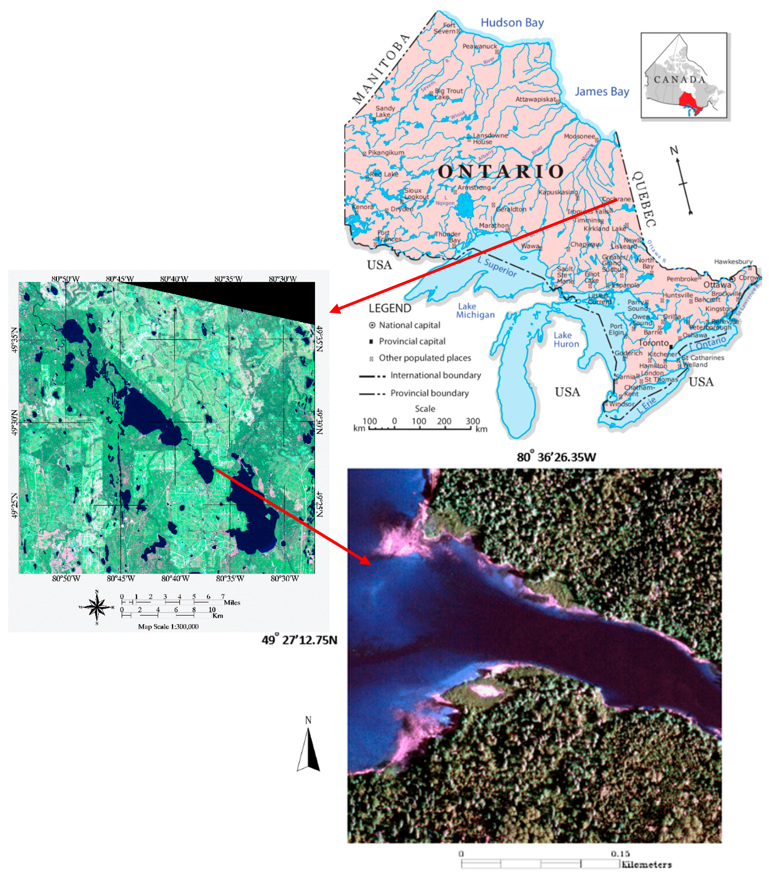
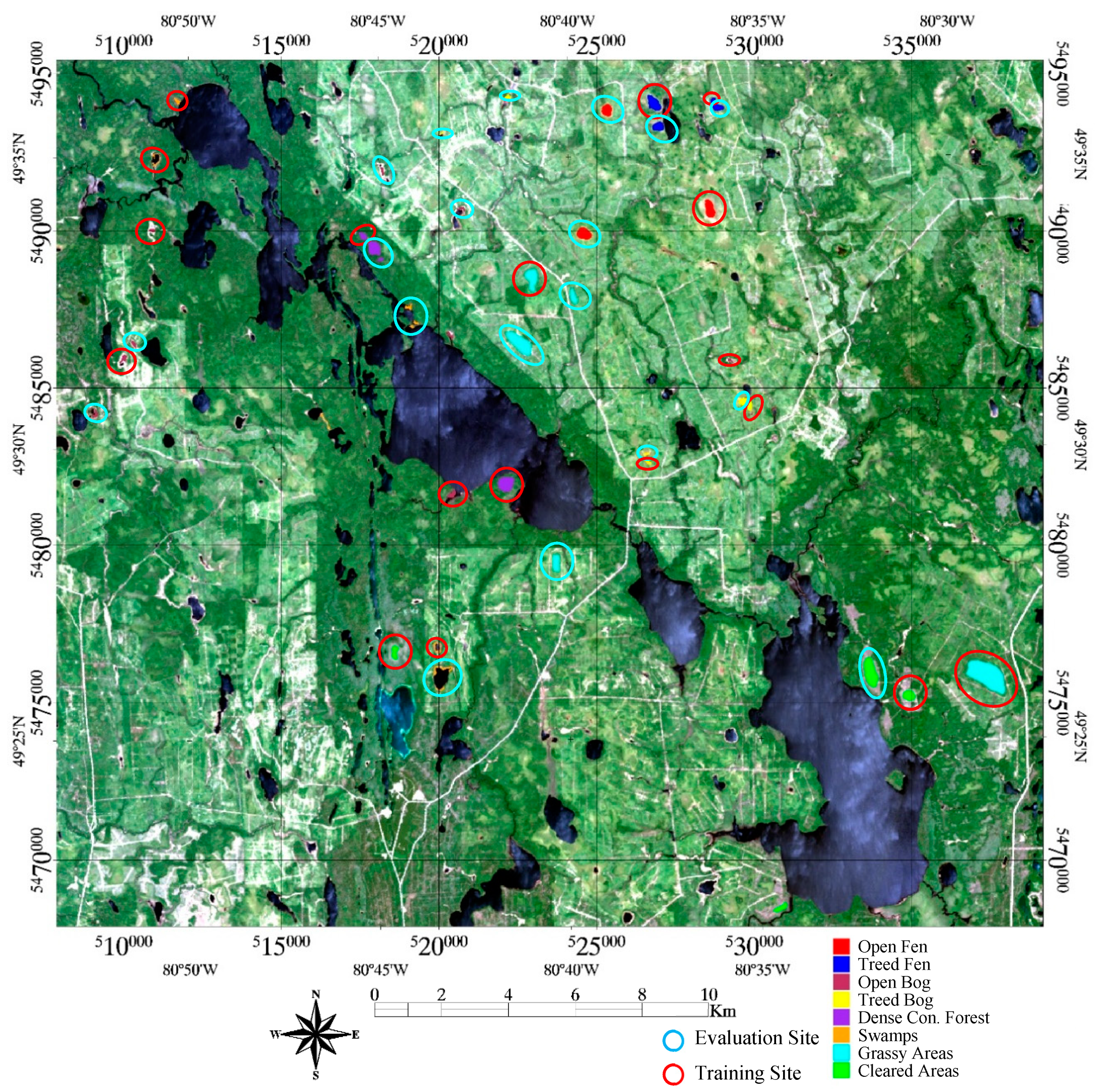
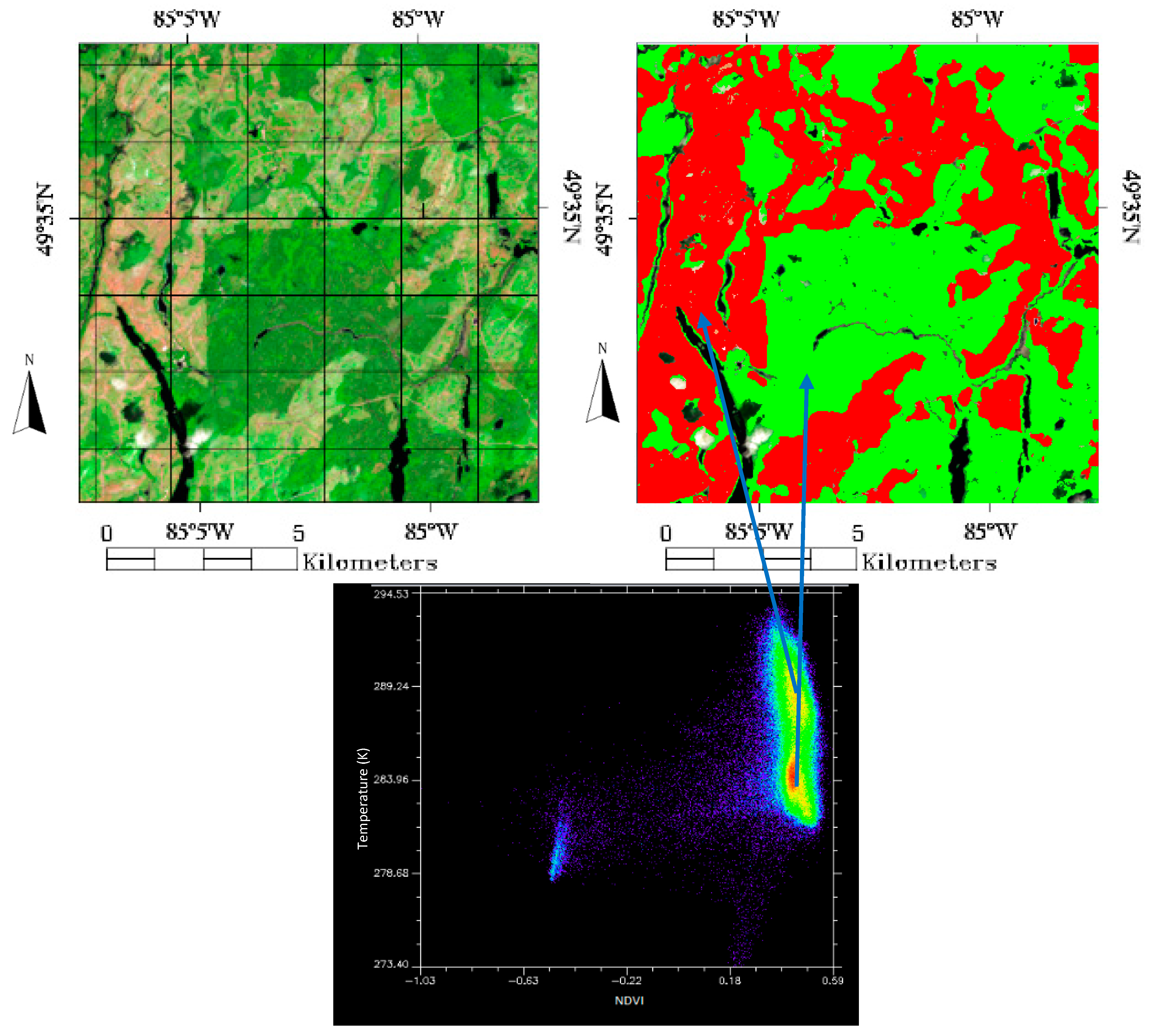
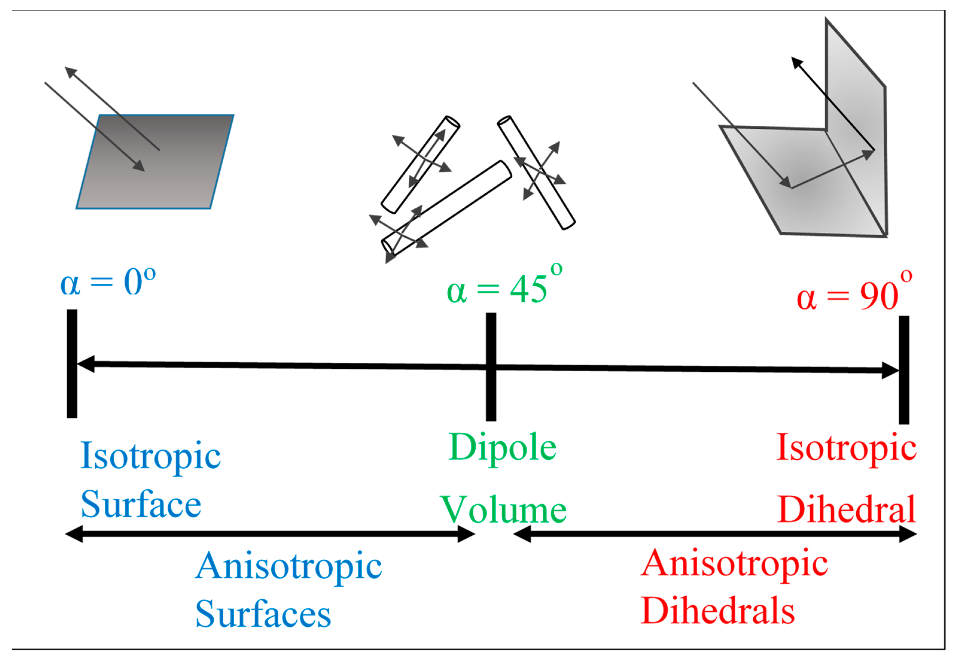
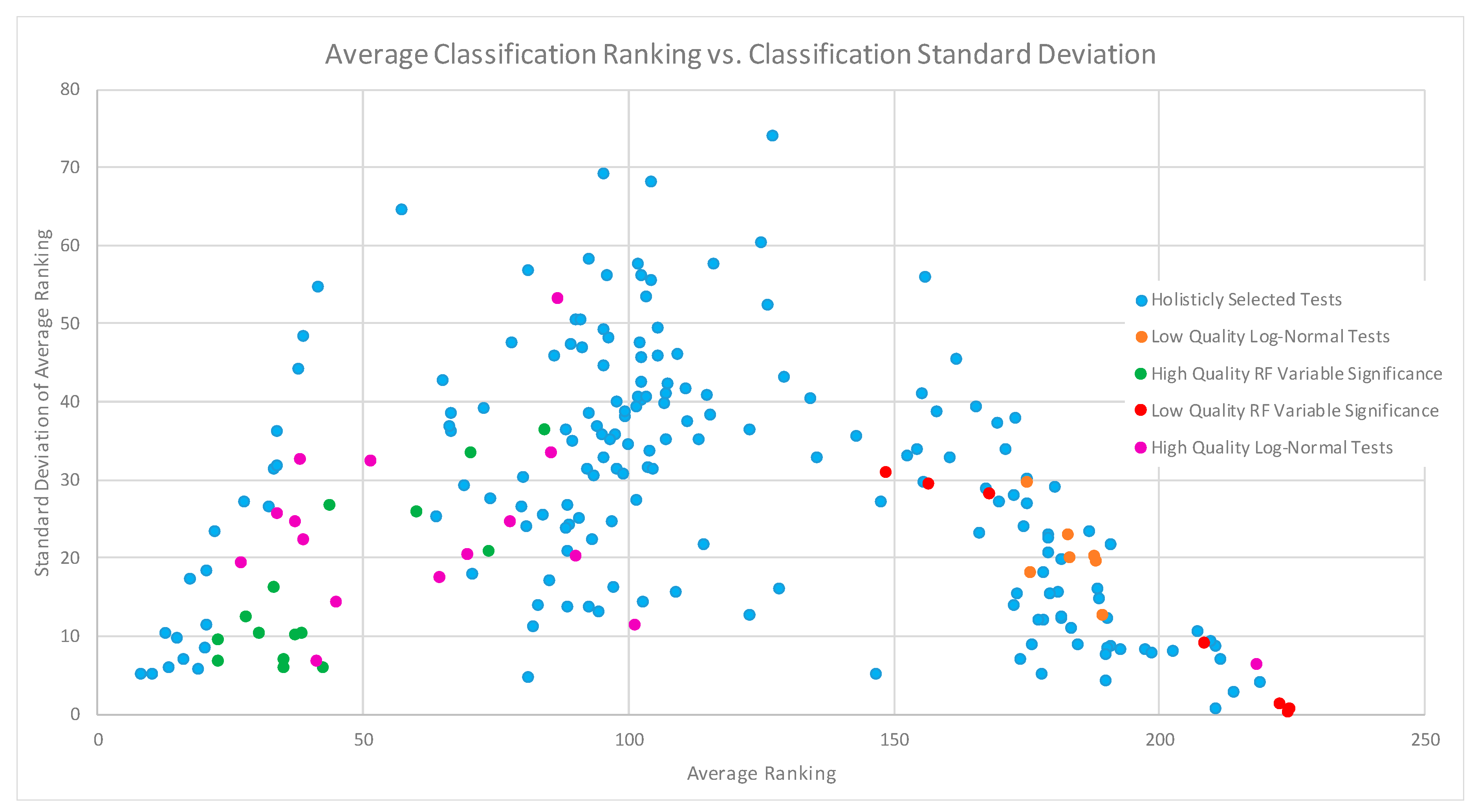
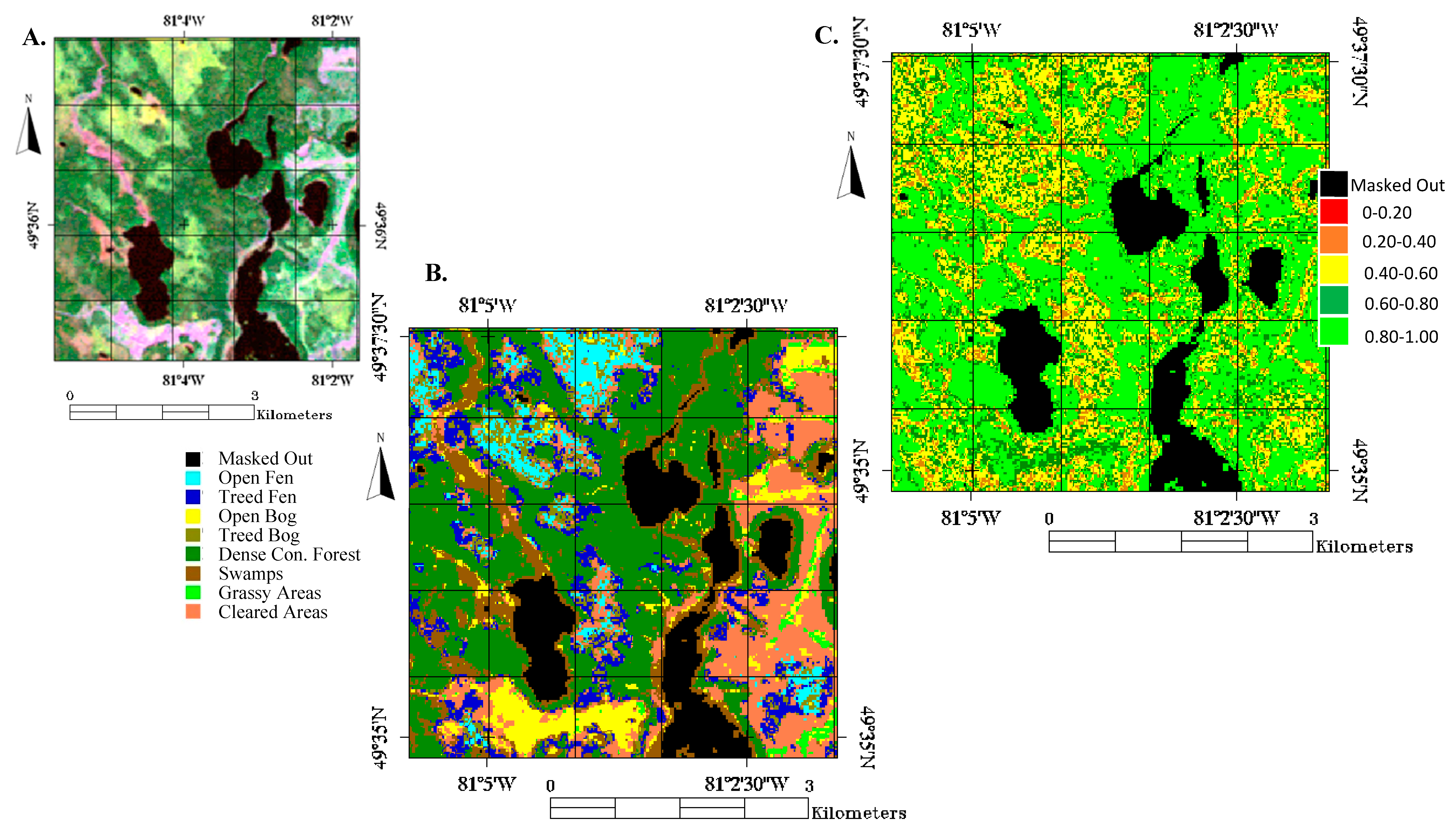
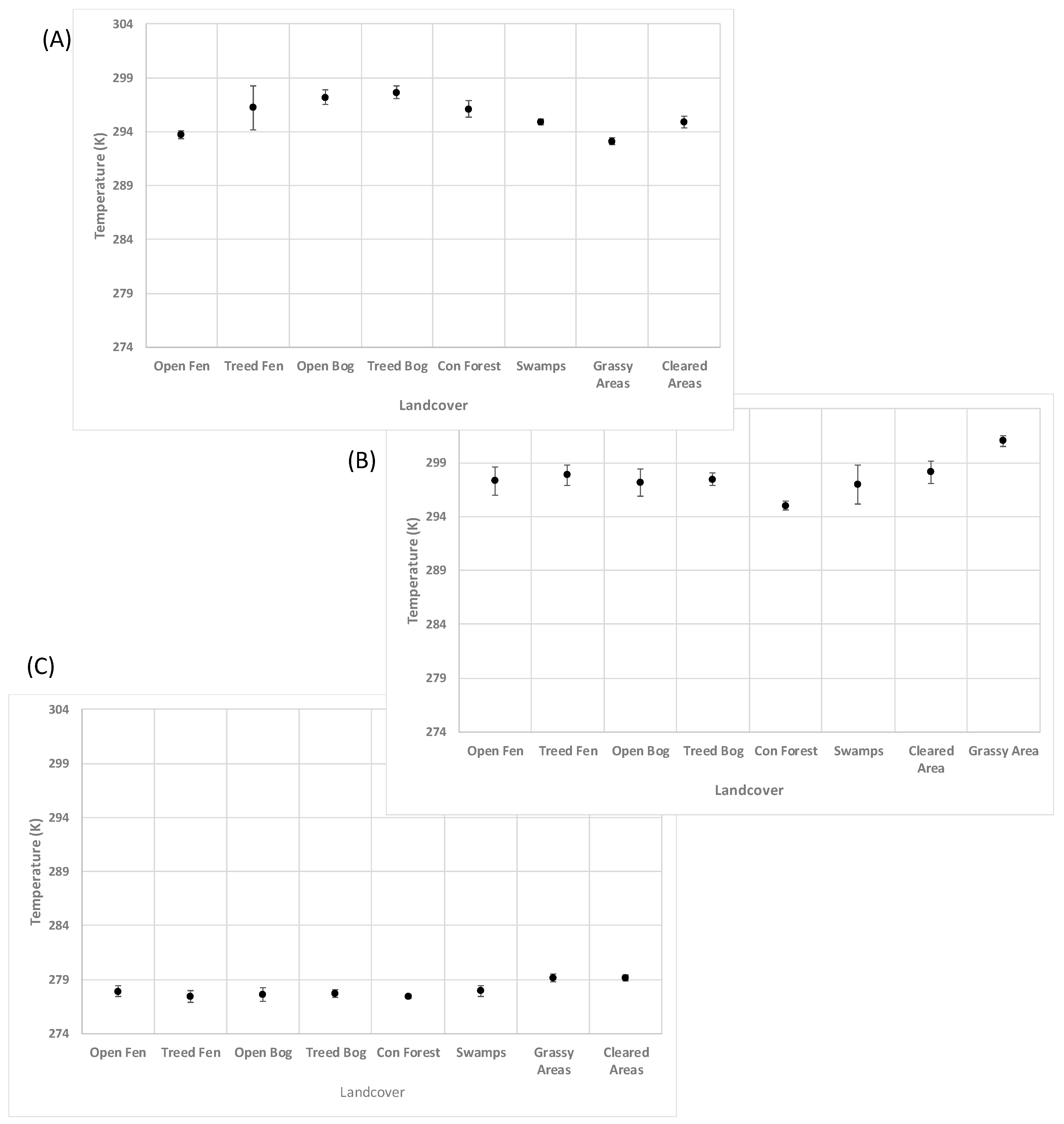
Table 1.
Summary of remotely-sensed imagery collected for this study.
| Imagery | Season | Date | Level of Processing | Accessed From | |
|---|---|---|---|---|---|
| 1. | Landsat-5 | Spring-1 | 18-May-2010 | Level 1G | United States Geological Survey (USGS) |
| 2. | Landsat-5 | Spring-2 | 15-May-2009 | Level 1G | USGS |
| 3. | RADARSAT-2 | Summer-1 | 29-June-2014 | Level 1—Single Look Complex (SLC) | Canadian Space Agency (CSA) |
| 4. | Landsat-5 | Summer-2 | 24-July-2011 | Level 1G | USGS |
| 5. | Sentinel-1 | Summer-1 | 01-August-2015 | Level 1—SLC | European Space Agency (ESA) - Sentinel |
| 6. | Sentinel-1 | Summer-2 | 25-August-2015 | Level 1—SLC | ESA - Sentinel |
| 7. | RADARSAT-2 | Fall-1 | 10-October-2014 | Level 1—SLC | CSA |
| 8. | Landsat-5 | Fall-1 | 09-October-2010 | Level 1G | USGS |
| 9. | Landsat-5 | Fall-2 | 10-November-2010 | Level 1G | USGS |
| 10. | Sentinel-1 | Fall-1 | 18-September-2015 | Level 1—SLC | ESA - Sentinel |
Table 2.
Number of pixels used for different classes in training and testing.
| Class | Number Assigned to Class | Number of Pixels in Training Set | Number of Pixels in Validation Set |
|---|---|---|---|
| Open Fen | Class 1 | 839 | 624 |
| Treed Fen | Class 2 | 766 | 526 |
| Open Bog | Class 3 | 802 | 517 |
| Treed Bog | Class 4 | 868 | 563 |
| Dense Con. Forest | Class 5 | 933 | 672 |
| Swamps | Class 6 | 881 | 580 |
| Grassy Areas | Class 7 | 2541 | 1331 |
| Cleared Areas | Class 8 | 3184 | 2147 |
Table 3.
Image Input features used during this study and their associated variable index.
| Index | Feature Name | Index | Feature Name | Index | Feature Name | Index | Feature Name |
|---|---|---|---|---|---|---|---|
| 1 | B1 Reflect. Spring 1 | 13 | B1 Reflect. Summer 2 | 25 | B1 Reflect. Fall 1 | 37 | Sentinel VV - Summer 1 |
| 2 | B2 Reflect. Spring 1 | 14 | B2 Reflect. Summer 2 | 26 | B2 Reflect. Fall 1 | 38 | Sentinel VH - Summer 1 |
| 3 | B3 Reflect. Spring 1 | 15 | B3 Reflect. Summer 2 | 27 | B3 Reflect. Fall 1 | 39 | Sentinel VV - Summer 2 |
| 4 | B4 Reflect. Spring 1 | 16 | B4 Reflect. Summer 2 | 28 | B4 Reflect. Fall 1 | 40 | Sentinel VH - Summer 2 |
| 5 | B5 Reflect. Spring 1 | 17 | B5 Reflect. Summer 2 | 29 | B5 Reflect. Fall 1 | 41 | Sentinel VV - Fall 1 |
| 6 | B6 Reflect. Spring 1 | 18 | B6 Reflect. Summer 2 | 30 | B6 Reflect. Fall 1 | 42 | Sentinel VH - Fall 1 |
| 7 | B7 Reflect. Spring 1 | 19 | B7 Reflect. Summer 2 | 31 | B7 Reflect. Fall 1 | 43 | Digital Elevation Map (DEM) |
| 8 | Temp Spring 1 | 20 | Temp Summer 1 | 32 | Temp Fall 1 | 44 | DEM-Slope |
| 9 | Temp Spring 2 | 21 | Temp Summer 2 | 33 | Temp Fall 2 | 45 | Entrophy Fall |
| 10 | NDVI Spring 1 | 22 | NDVI Summer 2 | 34 | NDVI Fall 1 | 46 | Alpha Fall |
| 11 | NDWI Spring 1 | 23 | NDWI Summer 2 | 35 | NDWI Fall 1 | 47 | Entrophy Summer |
| 12 | Albedo Spring 1 | 24 | Albedo Summer 2 | 36 | Albedo Fall 1 | 48 | Alpha Summer |
Table 4.
(Top) Summary of image feature quality analysis averaged over all land cover types. Image metrics, image bands, radar parameters, DEM and slope sorted from largest to smallest log-normal distance, with a longer distance implying a higher quality. (Bottom) Summary of image feature importance values computed through and averaged over 47 unique RF tests.
| Log-Normal Distance | |||||
|---|---|---|---|---|---|
| Bands | Distance | Metrics | Distance | Radar and DEM | Distance |
| B4 Reflect. Summer 2 | 1.876 | NDVI Summer 2 | 1.826 | DEM | 1.311 |
| B7 Reflect. Spring 1 | 1.473 | Temp Summer 2 | 1.507 | Entrophy Fall | 0.556 |
| B5 Reflect. Spring 1 | 1.187 | NDVI Spring 1 | 1.400 | Alpha Fall | 0.530 |
| B6 Reflect. Spring 1 | 1.160 | Temp Spring 1 | 1.374 | DEM-Slope | 0.426 |
| B4 Reflect. Reflect. Fall 1 | 1.140 | Temp Summer 1 | 1.370 | Alpha Summer | 0.133 |
| B7 Reflect. Summer 2 | 1.069 | Temp Spring 2 | 1.355 | Entrophy Summer | 0.101 |
| B2 Reflect. Fall 1 | 0.965 | Albedo Summer 2 | 1.339 | Sentinel VH - Summer 1 | 0.047 |
| B6 Reflect. Summer 2 | 0.932 | Temp Fall 2 | 1.220 | Sentinel VV - Summer 1 | 0.043 |
| B4 Reflect. Reflect. Spring 1 | 0.910 | NDVI Fall 1 | 1.219 | Sentinel VH - Fall 1 | 0.030 |
| B1 Reflect. Fall 1 | 0.889 | Temp Fall 1 | 1.210 | Sentinel VV - Fall 1 | 0.030 |
| B7 Reflect. Fall 1 | 0.884 | NDWI Spring 1 | 1.086 | Sentinel VH - Summer 2 | 0.027 |
| B2 Reflect. Summer 2 | 0.881 | Albedo Fall 1 | 0.866 | Sentinel VV - Summer 2 | 0.025 |
| B5 Reflect. Summer 2 | 0.874 | Albedo Spring 1 | 0.863 | ||
| B6 Reflect. Fall 1 | 0.861 | NDWI Summer 2 | 0.859 | ||
| B3 Reflect. Summer 2 | 0.853 | NDWI Fall 1 | 0.607 | ||
| B2 Reflect. Spring 1 | 0.823 | ||||
| B1 Reflect. Spring 1 | 0.774 | ||||
| B3 Reflect. Fall 1 | 0.712 | ||||
| B3 Reflect. Spring 1 | 0.679 | ||||
| B1 Reflect. Summer 2 | 0.658 | ||||
| B5 Reflect. Fall 1 | 0.647 | ||||
| Average | 0.964 | Average | 1.207 | Average | 0.272 |
| Standard Deviation | 0.282 | Standard Deviation | 0.298 | Standard Deviation | 0.370 |
| Bands | Distance | Metrics | Distance | Radar and DEM | Distance |
| B1 Reflect. Fall 1 | 1.083 | NDVI Fall 1 | 1.654 | DEM | 1.350 |
| B5 Reflect. Spring 1 | 0.945 | NDVI Summer 2 | 1.450 | DEM-Slope | 0.810 |
| B4 Reflect. Summer 2 | 0.891 | Temp Spring 1 | 1.262 | Entrophy Fall | 0.800 |
| B1 Reflect. Summer 2 | 0.827 | NDVI Spring 1 | 1.261 | Alpha Summer | 0.770 |
| B4 Reflect. Fall 1 | 0.821 | Temp Spring 2 | 1.246 | Entrophy Summer | 0.748 |
| B7 Reflect. Summer 2 | 0.799 | Temp Summer 1 | 1.139 | Alpha Fall | 0.588 |
| B7 Reflect. Fall 1 | 0.745 | NDWI Fall 1 | 1.126 | Sentinel VH - Summer 2 | 0.471 |
| B2 Reflect. Summer 2 | 0.725 | Temp Fall 1 | 0.980 | Sentinel VV - Fall 1 | 0.430 |
| B2 Reflect. Fall 1 | 0.717 | NDWI Spring 1 | 0.883 | Sentinel VV - Summer 2 | 0.394 |
| B7 Reflect. Spring 1 | 0.700 | Temp Summer 2 | 0.865 | Sentinel VH - Fall 1 | 0.376 |
| B6 Reflect. Spring 1 | 0.682 | Temp Fall 2 | 0.848 | Sentinel VV - Summer 1 | 0.334 |
| B1 Reflect. Spring 1 | 0.665 | NDWI Summer 2 | 0.655 | Sentinel VH - Summer 1 | 0.302 |
| B4 Reflect. Spring 1 | 0.620 | Albedo Summer 2 | 0.605 | ||
| B3 Reflect. Summer 2 | 0.600 | Albedo Spring 1 | 0.583 | ||
| B2 Reflect. Spring 1 | 0.597 | Albedo Fall 1 | 0.435 | ||
| B3 Reflect. Spring 1 | 0.588 | ||||
| B6 Reflect. Summer 2 | 0.563 | ||||
| B6 Reflect. Fall 1 | 0.557 | ||||
| B5 Reflect. Fall 1 | 0.544 | ||||
| B5 Reflect. Summer 2 | 0.502 | ||||
| B3 Reflect. Fall 1 | 0.356 | ||||
| Average | 0.692 | Average | 0.999 | Average | 0.614 |
| Standard Deviation | 0.161 | Standard Deviation | 0.335 | Standard Deviation | 0.288 |
Table 5.
Summary of classification accuracy of different methodologies averaged over all classification strategies.
Table 5.
Summary of classification accuracy of different methodologies averaged over all classification strategies.
| Average | Standard Deviation | Max | Min | Ave. Kappa Value | Difference from Top to 25th Percentile | Difference from Top to 50th Percentile | Computation Time (s) | |
|---|---|---|---|---|---|---|---|---|
| Random Forest Classifier | 0.7127 | 0.0838 | 0.8751 | 0.3608 | 0.7341 | 0.1101 | 0.1528 | 2314 |
| Support Vector Machine | 0.6528 | 0.0785 | 0.8004 | 0.3979 | 0.7171 | 0.0891 | 0.1424 | 838 |
| K-Nearest Neighbor Classifier | 0.6210 | 0.0791 | 0.7746 | 0.2217 | 0.7218 | 0.1002 | 0.1407 | 364 |
| Naive Bayes | 0.5913 | 0.0643 | 0.6998 | 0.3105 | 0.7025 | 0.0567 | 0.0913 | 26 |
Table 6.
Summary of best overall performing input features for individual classification methodologies.
Table 6.
Summary of best overall performing input features for individual classification methodologies.
| Random Forest Classifier | Support Vector Machine | K-Nearest Neighbor Classifier | Naive Bayes | |
|---|---|---|---|---|
| Image Reflectance | X | X | X | X |
| NDVI | X | X | X | |
| NDWI | X | |||
| Albedo | ||||
| Surface Temperature | X | X | X | X |
| RADARSAT-2 | X | X | ||
| Sentinel-1 | X | |||
| DEM | X | X | ||
| DEM - Slope | X | X | ||
| Spring | ||||
| Summer | ||||
| Fall | ||||
| All season in Combination | X | X | X | X |
Table 7.
Summary of the lowest performing input feature combinations for individual classification methodologies.
Table 7.
Summary of the lowest performing input feature combinations for individual classification methodologies.
| Random Forest Classifier | Support Vector Machine | K-Nearest Neighbor Classifier | Naive Bayes | |
|---|---|---|---|---|
| Image Reflectance | ||||
| NDVI | Fall data only | Fall data only | Fall data only | Spring and Fall data |
| NDWI | Fall data only | Fall data only | Fall data only | Spring and Fall data |
| Albedo | Fall data only | Fall data only | Fall data only | Spring and Fall data |
| Surface Temperature | Fall data only | |||
| RADARSAT-2 | Fall data only | Fall data only | ||
| Sentinel-1 | Fall data only | |||
| DEM | X | |||
| DEM—Slope | X | |||
| Spring | ||||
| Summer | ||||
| Fall | X | X | X | X |
| All seasons in Combination |
Table 8.
Confusion matrix of the best performing classification test (RF test #77).
| Grassy Area | Treed Bog | Cleared Area | Treed Fen | Open Bog | Open Fen | Swamps | Coniferous Forest | Producer Accuracy | User Accuracy | |
|---|---|---|---|---|---|---|---|---|---|---|
| Grassy Area | 582 | 0 | 0 | 39 | 0 | 0 | 0 | 0 | 0.937 | 0.909 |
| Treed Bog | 56 | 247 | 7 | 5 | 0 | 0 | 0 | 0 | 0.784 | 0.969 |
| Cleared Area | 0 | 0 | 219 | 0 | 0 | 157 | 0 | 0 | 0.582 | 0.969 |
| Treed Fen | 2 | 8 | 0 | 299 | 0 | 0 | 12 | 0 | 0.932 | 0.872 |
| Open Bog | 0 | 0 | 0 | 0 | 794 | 84 | 0 | 0 | 0.904 | 0.951 |
| Open Fen | 0 | 0 | 0 | 0 | 41 | 341 | 0 | 0 | 0.893 | 0.580 |
| Swamps | 0 | 0 | 0 | 0 | 0 | 6 | 3109 | 4 | 0.997 | 0.985 |
| Coniferous Forest | 0 | 0 | 0 | 0 | 0 | 0 | 35 | 1142 | 0.970 | 0.997 |
Table 9.
Confusion matrix of the worst performing classification test (Naïve Bayes test #225).
| Grassy Area | Treed Bog | Cleared Area | Treed Fen | Open Bog | Open Fen | Swamps | Coniferous Forest | Producer Accuracy | User Accuracy | |
|---|---|---|---|---|---|---|---|---|---|---|
| Grassy Area | 206 | 26 | 85 | 56 | 0 | 51 | 167 | 30 | 0.332 | 0.516 |
| Treed Bog | 63 | 50 | 27 | 29 | 0 | 27 | 89 | 30 | 0.159 | 0.211 |
| Cleared Area | 9 | 15 | 40 | 15 | 19 | 28 | 162 | 88 | 0.106 | 0.145 |
| Treed Fen | 50 | 32 | 16 | 28 | 7 | 12 | 131 | 45 | 0.087 | 0.130 |
| Open Bog | 2 | 7 | 9 | 3 | 387 | 27 | 373 | 70 | 0.441 | 0.385 |
| Open Fen | 20 | 10 | 56 | 17 | 72 | 55 | 106 | 46 | 0.144 | 0.154 |
| Swamps | 10 | 49 | 27 | 29 | 485 | 105 | 1871 | 539 | 0.601 | 0.533 |
| Coniferous Forest | 39 | 48 | 16 | 38 | 35 | 51 | 614 | 340 | 0.288 | 0.286 |
© 2019 by the authors. Licensee MDPI, Basel, Switzerland. This article is an open access article distributed under the terms and conditions of the Creative Commons Attribution (CC BY) license (http://creativecommons.org/licenses/by/4.0/).
Share and Cite
MDPI and ACS Style
Judah, A.; Hu, B. The Integration of Multi-source Remotely-Sensed Data in Support of the Classification of Wetlands. Remote Sens. 2019, 11, 1537. https://0-doi-org.brum.beds.ac.uk/10.3390/rs11131537
AMA Style
Judah A, Hu B. The Integration of Multi-source Remotely-Sensed Data in Support of the Classification of Wetlands. Remote Sensing. 2019; 11(13):1537. https://0-doi-org.brum.beds.ac.uk/10.3390/rs11131537
Chicago/Turabian StyleJudah, Aaron, and Baoxin Hu. 2019. "The Integration of Multi-source Remotely-Sensed Data in Support of the Classification of Wetlands" Remote Sensing 11, no. 13: 1537. https://0-doi-org.brum.beds.ac.uk/10.3390/rs11131537
Note that from the first issue of 2016, this journal uses article numbers instead of page numbers. See further details here.