Evaluation of Vegetation Biophysical Variables Time Series Derived from Synthetic Sentinel-2 Images

Canada Center for Remote Sensing, Canada Centre for Mapping and Earth Observation, Natural Resources Canada, 6th Floor, 560 Rochester Street, Ottawa, ON K1A 0E4, Canada
*
Author to whom correspondence should be addressed.
Remote Sens. 2019, 11(13), 1547; https://0-doi-org.brum.beds.ac.uk/10.3390/rs11131547
Submission received: 22 May 2019
/
Revised: 19 June 2019
/
Accepted: 26 June 2019
/
Published: 29 June 2019
(This article belongs to the Special Issue Advances of Multi-Temporal Remote Sensing in Vegetation and Agriculture Research)
Abstract
:Time series of vegetation biophysical variables (leaf area index (LAI), fraction canopy cover (FCOVER), fraction of absorbed photosynthetically active radiation (FAPAR), canopy chlorophyll content (CCC), and canopy water content (CWC)) were estimated from interpolated Sentinel-2 (S2-LIKE) surface reflectance images, for an agricultural region located in central Canada, using the Simplified Level 2 Product Prototype Processor (SL2P). S2-LIKE surface reflectance data were generated by blending clear-sky Sentinel-2 Multispectral Imager (S2-MSI) images with daily BRDF-adjusted Moderate Resolution Imaging Spectrometer images using the Prediction Smooth Reflectance Fusion Model (PSFRM), and validated using thirteen independent S2-MSI images (RMSE 6%). The uncertainty of S2-LIKE surface reflectance data increases with the time delay between the prediction date and the closest S2-MSI image used for training PSFRM. Vegetation biophysical variables from S2-LIKE products are validated qualitatively and quantitatively by comparison to the corresponding vegetation biophysical variables from S2-MSI products (RMSE = 0.55 for LAI, ~10% for FCOVER and FAPAR, and 0.13 g/m2 for CCC and 0.16 kg/m2 for CWC). Uncertainties of vegetation biophysical variables derived from S2-LIKE products are almost linearly related to the uncertainty of the input reflectance data. When compared to the in situ measurements collected during the Soil Moisture Active Passive Validation Experiment 2016 field campaign, uncertainties of LAI (0.83) and FCOVER (13.73%) estimates from S2-LIKE products were slightly larger than uncertainties of LAI (0.57) and FCOVER (11.80%) estimates from S2-MSI products. However, equal uncertainties (0.32 kg/m2) were obtained for CWC estimates using SL2P with either S2-LIKE or S2-MSI input data.
Keywords:
vegetation biophysical variables; time series; medium resolution; S2-LIKE; S2-MSI; MODIS/NBAR; PSRFM; SL2P
1. Introduction
There is international consensus as to the need for global medium resolution (<100 m) mapping of vegetation biophysical variables at subweekly temporal frequency [1,2,3]. For agriculture, this requirement is supplemented by the need to monitor the rapid change in the state of vegetation due to plant growth, management practices, water stress, pests and disease [4]. The Global Climate Observing System [3] and expert panels [2,5] have identified medium and high-resolution space borne multispectral imagers as a suitable source of satellite data records from which products meeting mapping requirements could be derived. The revisit period of multispectral imagers providing systematic global coverage is generally larger than 10 days at the Equator [6]. The ability to meet temporal requirements for mapping is further limited by cloud cover, with a global average probability of 0.7 and substantial temporal persistence between days [7]. These constraints indicate that mapping vegetation biophysical variables at subweekly intervals will require algorithms applicable to a constellation of satellite imagers that together allow for subweekly medium or high resolution estimates of required input reflectance.
The Sentinel-2 (S2) constellation (S2A and S2B satellites), designed to provide satellite data that can be used to globally map land surface variables, provides systematic observations with increased temporal resolutions in comparison to many current medium resolution optical satellite sensors [8]. Together, S2A and S2B provide better than 5-day revisit of the Earth’s land using a virtually identical decametric (10–20 m) resolution Multispectral Imager (MSI) [8]. The Simplified L2 Product Prototype Processor 2 (SL2P) can systematically derive five vegetation biophysical variables from MSI surface reflectance data: Leaf Area Index (LAI), Fraction of canopy Cover (FCOVER), Fraction of Absorbed Photosynthetically Active Radiation (FAPAR), Canopy Chlorophyll Concentration (CCC), and Canopy Water Content (CWC) [9]. Recent validation studies indicated that SL2P estimates of LAI, FAPAR, and FCOVER using S2-MSI imagery approach user requirements; CCC and CWC exhibit substantial bias although their uncertainty (including accuracy) is typically within user requirements [10,11].
Notwithstanding the adequacy of the spectral and spatial characteristics of S2-MSI data or SL2P performance, Djamai et al. [11] showed that the revisit period of the data acquired by a constellation of S2A and the Landsat-8 Operation Land Imager (S2B was not operational at that time) was insufficient to derive cloud-free subweekly observations during the critical growth stages of crops over a study region in central Canada. Wulder et al. [12] similarly report a range of ~5 to ~23 cloud-free acquisitions from a virtual constellation of Landsat, S2A and S2B sensors over Canada during the growing season. Given the potential for reduced cloud-free observations in more cloudy areas or areas closer to the equator, there is a need to increase the temporal frequency of estimates of biophysical parameters from MSI measurements. Ideally, one would include additional satellites that meet spectral and spatial resolution requirements [13]. However, such a constellation of medium resolution imagers having similar spectral bands as the MSI and with systematic global acquisition does not currently exist. Moreover, even with the current S2A and S2B constellation, there is always the possibility of a malfunction of one of S2A or S2B. In this case, it may be critical to provide a high temporal revisit data stream for services that have built a reliance on such data. It is therefore necessary to evaluate the possibility of using constellations that include sensors with coarse (>100 m) spatial resolution but higher temporal revisit and systematic global coverage. Subsequently, there is a need to develop and evaluate algorithms capable of estimating vegetation biophysical variables by combining frequent revisit coarse resolution observations with data from the S2 constellation and to quantify the uncertainty of these estimates in comparison to either estimates from using only single date S2-MSI imagery or from reference in situ measurements.
Both model based and statistical approaches have been tested for estimating biophysical variables through a combination of imagery with different spatial resolution and spectral bands. Model based approaches rely on a land surface model relating required vegetation biophysical variables to either top-of-canopy or top-of-atmosphere reflectance at the spatial and spectral resolution of each sensor and an algorithm for updating the model to match observations from multiple sensors. Such algorithms are often based on data assimilation techniques [14,15,16] that may result in effective variables in the case of model error or simplification or due to error in forcing [17]. Statistical data fusion approaches rely on data driven relationships to produce synthetic parameter maps based on combinations of images from multiple sensors [14,18]. The statistical relationship can either be developed to combine products or input reflectance quantities. Here we use a statistical data driven method that combines input reflectance for two reasons:
- The relationship between input reflectance and vegetation parameters is scale-dependent [19] so one would need to develop and characterize retrieval algorithms for each sensor if products were to be combined.
- We use a linear algorithm for combining reflectance quantities [20] that we hypothesize will result in linear estimation errors of both reflectance as a function of differences between actual and assumed temporal changes. In this case, the reflectance estimation error will be a function of the temporal interpolation interval duration during periods of monotonic change in reflectance.
Statistical data fusion approaches are widely used for predicting surface reflectance data from clear-sky Landsat and Moderate Resolution Imaging Spectroradiometer (MODIS) images [21]. The Prediction Smooth Reflectance Fusion Model (PSRFM) for blending Landsat and MODIS images [20] is used here as it showed lower uncertainty in comparison to Spatial and Temporal Adaptive Reflectance Fusion Model (STARFM) [22] and Enhanced version of STARFM (ESTARFM) [23] over a mixed land cover region in central Canada [20]. As a result, PSRFM was adapted to S2-MSI and applied to clear-sky S2-MSI images and daily Nadir BRDF adjusted MODIS products (MCD43A4) to produce daily synthetic S2-LIKE surface reflectance images. Subsequently, SL2P was employed to estimate vegetation biophysical variables (LAI, FCOVER, FAPAR, CCC and CWC) from the S2-LIKE surface reflectance images.
Previous studies have tested ESTARFM for blending coarse and fine resolution LAI products [24,25,26,27]. This approach will include both the additional uncertainty within the coarse resolution LAI algorithm, that also must be specified for use in ESTARFM, and more importantly does not simultaneously retrieve multiple biophysical parameters in a consistent manner. Dong et al. [28] used ESTARFM to estimate LAI from interpolated reflectance using an empirical vegetation index relationship specific to wheat but validated modelled biomass rather than estimated LAI. Our study is novel in that (i) it uses PSFRM that has been shown by [20] to have lower reflectance prediction uncertainty than ESTARFM (ii) it uses globally applicable algorithms (Sen2COR and SL2P) rather than a local empirical algorithm (iii) both the algorithms and their validation are applied to multiple simultaneously derived parameters as may be required, for example, by crop models (iv) it validates both reflectance and parameter estimates over a range of different crop types in a mixed land cover region that, in principle, should be more challenging for calibration of PSFRM than areas with relatively uniform cover. In this sense, our study addresses two research questions:
- Can we retrieve vegetation biophysical variables from synthetic S2-LIKE images with subweekly frequency in mid-latitude regions?
- What is the uncertainty of vegetation biophysical variables estimates from S2-LIKE images compared to estimates from S2-MSI images and in situ data and how does the uncertainty change with temporal gap size.
The study period spans the growing season of a number of crop types from emergence to pre-growth then to senescence /harvest; although in situ validation is limited to the first two phases due to the available field data (also used in [11]). Considering that SL2P uncertainty is substantially larger than the uncertainty (<5%) reported for PSFRM we hypothesize that, when interpolating within a subweekly interval, vegetation biophysical variables estimated from synthetic S2-LIKE images will agree with estimates from S2-MSI images within the uncertainty of biophysical variable estimates from these latter images. Further, considering that PSFRM assumes a linear spectral relationship between the calibration image and the prediction image we hypothesize that this estimation uncertainty will generally be proportional to elapsed time to the nearest S2-MSI scene used for PSRFM model training.
2. Study Area and Datasets
2.1. Study Area
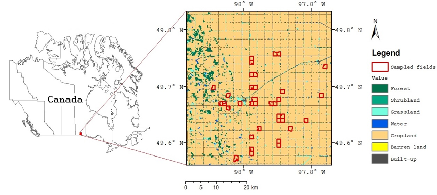
The study area is located in Manitoba province of Canada, between the latitudes 49.56°N and 49.83°N and longitudes 97.75°W and 98.16°W and ~230 m above sea level (Figure 1). It is predominantly flat with more than 95% cropland and grassland cover. The area was selected since crops and grasses can exhibit large spatial and temporal variability in vegetation variables during the growing season and because of the availability of in situ measurements of three variables (FCOVER, LAI and CWC).
2.2. S2-MSI Images
Only images from S2-A were used as S2-B was not operational during the study period. S2-A provides a ~10-day revisit cycle with an equatorial overpass time at approximately 10:30 a.m. (descending node) [8]. Table 1 provides details about S2-MSI spectral bands used for estimating vegetation biophysical variables using SL2P processor. More details about S2-MSI are provided at Sentinel-2 dedicated web site [30].
2.3. MODIS Images
The MCD43A4 Version 6 Nadir Bidirectional Reflectance Distribution Function (BRDF) adjusted reflectance (NBAR) daily product was used for this study [31]. MCD43A4 is a 16-day combined product providing 500 m reflectance data at bands designed for land applications (Table 2) and adjusted using the bidirectional reflectance distribution function to model the values as if they were collected from a nominal local solar zenith angle of the daily overpass [31]. Each pixel is the representative bidirectional reflectance value from combined MODIS acquisitions on Terra and Aqua satellites, for nadir view and solar position corresponding to the local overpass time, during the 16-day retrieval period. A quality assurance flag for each retrieval indicates if the estimate is processed using the primary algorithm, processed using an algorithm that matches directional albedo only, or not processed. Here, all processed retrievals were used as the retrievals from both the full inversion and magnitude inversion exhibit good linear relationships with observations [31]. Daily MCD43A4 images from 1 May 2016 to 30 September 2016 (151 images) were downloaded from United States Geological Survey (USGS) Earth Explore Data Portal [32].
2.4. In Situ Measurements
In situ measurements of LAI, FCOVER and CWC were collected during the SMAP Validation Experiment 2016 (SMAPVEX16-MB) [33] from 8 and 20 June and 10 to 22 July 2016. Among SMAPVEX16-MB in situ measurement days, three dates match with clear-sky S2-MSI acquisitions (Table 2). Thirty-seven (37) sampled fields, with dimensions of ~800 m × 800 m, within the study area are considered for this study (Figure 1). For each field, measurements were acquired at three Elementary Sampling Units (ESU) evenly distributed and located at more than 100 m away from the field edge.
LAI and FCOVER were estimated from digital hemispherical photographs using CanEye Version 5.1 following the SMAPVEX16-MB protocol [34] that corresponds in turn to the CCRS protocol for crops [35]. For each ESU, seven downward looking photos were captured from above the canopy using a Digital Hemispheric Photos (DHP) camera with a fish eye lens every 5 m along each of two parallel transects spaced 5 m apart. All the 14 photos were processed together to provide one estimate of LAI and FCOVER per ESU.
CWC was determined using gravimetric methods [34]. One biomass sample was collected at each ESU. For canola, wheat, oats, and alfalfa all above-ground biomass within a 0.5 m × 0.5 m square was cut. However, for corn and beans, five plants along two rows were collected. Knowing the crop density, wet and dry weights were scaled to a 1 m × 1 m area. In situ CWC was estimated by subtracting dry weights from wet weight.
3. Methodology
3.1. Preprocessing of S2-MSI and MODIS Images
Three preprocessing steps on S2-MSI and MODIS images were performed prior to image fusion:
- Converting Top of Atmosphere (TOA) S2-MSI reflectance data to atmospherically corrected surface reflectance data using Sen2Cor processor (Version 2.4.0) [37]. Sen2Cor generates also a Scene Classification Map (SCL) that is used further to mask undesirable pixels from S2-MSI images (only pixels labeled as bare soil or vegetated were retained). S2-MSI and S2-LIKE products were only compared and validated over bare soil or vegetated pixels as identified in the corresponding SCL map.
- Reprojecting and resampling MODIS data to match the geographic coordinate system and spatial resolution (20 m) defined for S2-MSI data using the MODIS Projection Tool [38].
3.2. Blending Approach
PSRFM was applied to generate synthetic S2-LIKE surface reflectance data for the six matching spectral bands between S2-MSI and MODIS images (Table 1). Details regarding the PSFRM algorithm and its performance in comparison to other approaches and reference images are given in [20]. Here we provide a description of how PSRFM was applied over the study area.
PSFRM requires two pairs of input fine and coarse resolution calibration images (Start and End pairs) and uses different coarse resolution images to predict fine resolution images sampled in time between the calibration images. To represent realistic data gaps, separate reflectance prediction models were developed for each subperiods of three successive S2-MSI acquisitions. For example, DOY 122 and DOY 142 were used as the start and end dates when predicting DOY 125, S2-LIKE reflectance images, and later derived parameter maps were then compared to the S2-MSI surface reflectance image or, alternatively, the derived parameter maps for the prediction date. Due to the large fraction of cloud coverage of the image at DOY 202 (66%) and 245 (11%), S2-MSI images of these two dates were not used either as start or end image for PSRFM training. Hence, cloud-free pixels of these images are used only for evaluation. Table 2 (column 3) lists the Start–end dates for each prediction subperiod. The temporal period interval between the evaluated S2-LIKE images dates and the closest Start or End dates for the corresponding superior (noted Min_) is also provided (column 4).
The calibration process involves defining a spatial partition of coarse resolution pixels sharing similar land cover (or at least spectral characteristics) and fitting a linear transformation relating fine and coarse resolution spectra given the mixture of land cover partitions within each coarse resolution pixel. The calibration requires co-located cloud-free fine and coarse resolution measurements.
For each S2-LIKE image, surface reflectance was predicted using forward and backward temporal blending using the start and end images, respectively. We assumed that no land cover type changes occurred during each subperiod as was the case for our study area. ISODATA clustering with fifteen clusters was used to determine clusters on each Start and End image that were assumed to correspond to pixels with similar land cover. For each cluster (), the reflectance change rate () between the start or end date and the prediction date was determined by solving an equation system based on spectral linear mixing theory [21] and the least squares adjustment method [39]. The forward or backward reflectance estimate at date () of band at pixel location (x, y) belonging to was computed as a linear function of time delay with respect to the Start (S for forward processing) or End (E for backward processing) date () with intercept corresponding to the reflectance at date ():
After the forward and backward surface reflectance at each pixel were predicted, they were smoothed by the weighted average based on the time difference between the prediction date and start (or end) date, respectively.
For S2-MSI Red-edge bands () having no matching with MODIS spectral bands (Table 1), the surface reflectance data at given date () was interpolated from PSRFM-predicted Red (b4) and NIR (b8A) bands for the same date (Equation (2)):
is a calibration coefficient derived for each pixel at date t from the relationship between the reflectance values of bands , b4 and b8A at Start and End dates as described by Equation (3):
As PSFRM adapts to the land cover mixture, surface reflectance predictions were performed in the S2-LIKE image only at pixels where at least one of the fine resolution calibration images were cloud-free. The acquisition geometry of each S2-LIKE pixel was specified as the same as the matching (in time and space) MCD43A4 pixel.
3.3. Estimation of Vegetation Biophysical Variables
The Simplified Level 2 Processor (SL2P) algorithm [9] was employed to estimate vegetation biophysical variables from each S2-LIKE and S2-MSI surface reflectance image. SL2P was developed to systematically retrieve vegetation biophysical variables from a single S2-MSI pixel measurement. SL2P finds inverse solutions of canopy parameters given the surface reflectance at spectral bands provided in Table 2, together with acquisition geometry, using a backpropagation neural network trained using a database of globally representative canopy conditions populated using PROSAILH [40,41] canopy radiative transfer model simulations. For each surface reflectance input, SL2P outputs the expected value for LAI, FCOVER, FAPAR, CCC and CWC. More details about SL2P processor are presented in the Algorithm Theoretical Based Document [9].
3.4. Intercomparison and Validation Strategies
We quantitatively intercompared S2-LIKE surface reflectance with S2-MSI surface reflectance acquired on the same date. Further, we qualitatively and quantitatively intercompared vegetation SL2P biophysical variables maps estimated from S2-LIKE images against the corresponding SL2P vegetation biophysical variables maps from S2-MSI observations for the same date. For quantitative intercomparisons, we used density scatter plots with three statistical metrics: the root mean square error (RMSE) and the bias and slope of the linear of S2-MSI versus S2-LIKE estimates. We also analyzed the uncertainty of the synthetic S2-LIKE surface reflectance images according to the temporal interval (Min_), and the uncertainty of vegetation biophysical variables maps estimated from S2-LIKE images according to the uncertainties of inputs images.
In the second step, we validated vegetation biophysical variables estimated from S2-LIKE images using SL2P by comparison to in situ measurements acquired at the same date. We used scatter plots with the same statistical metrics used for intercomparison. We compared scatter plots and statistical metrics obtained for vegetation biophysical variables estimated from S2-LIKE surface reflectance images to scatter plots and statistical metrics obtained for the corresponding variables estimated from S2-MSI observations.
4. Results
4.1. Evaluation of Synthetic Surface Reflectance Images
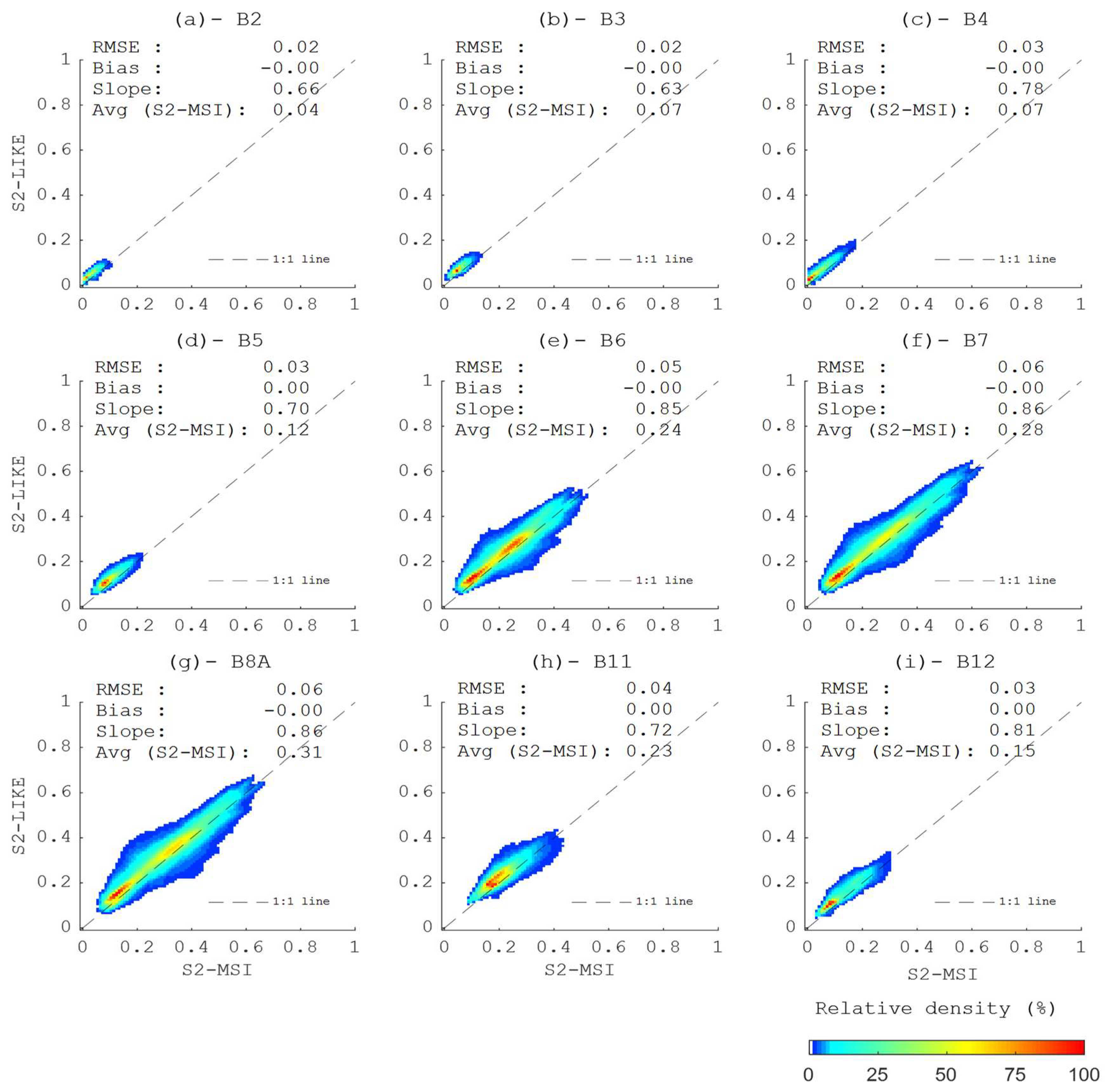
Figure 2 shows density scatter plots between S2-LIKE surface reflectance versus the corresponding S2-MSI surface reflectance for nine spectral bands. Reflectance data from all the images of 13 acquisition dates (Table 2) were merged for the evaluation. The graphs indicate that surface reflectance data from the synthetic S2-LIKE images compare well with the corresponding surface reflectance data from S2-MSI observations. Despite the low biases (0), slopes (from 0.65 to 0.85 for the different spectral bands) indicated a slight underestimation (overestimation) at high (low) reflectance. In terms of uncertainty, the RMSE between synthetic surface reflectance products and S2-MSI surface reflectance observations was below 6% for all the bands. The correlation coefficient between reflectance prediction error and S2-MSI view zenith angle was small (R2 between 0 and 0.08) indicating that the variation of S2-MSI view zenith angle had negligible effects on reflectance prediction uncertainty.
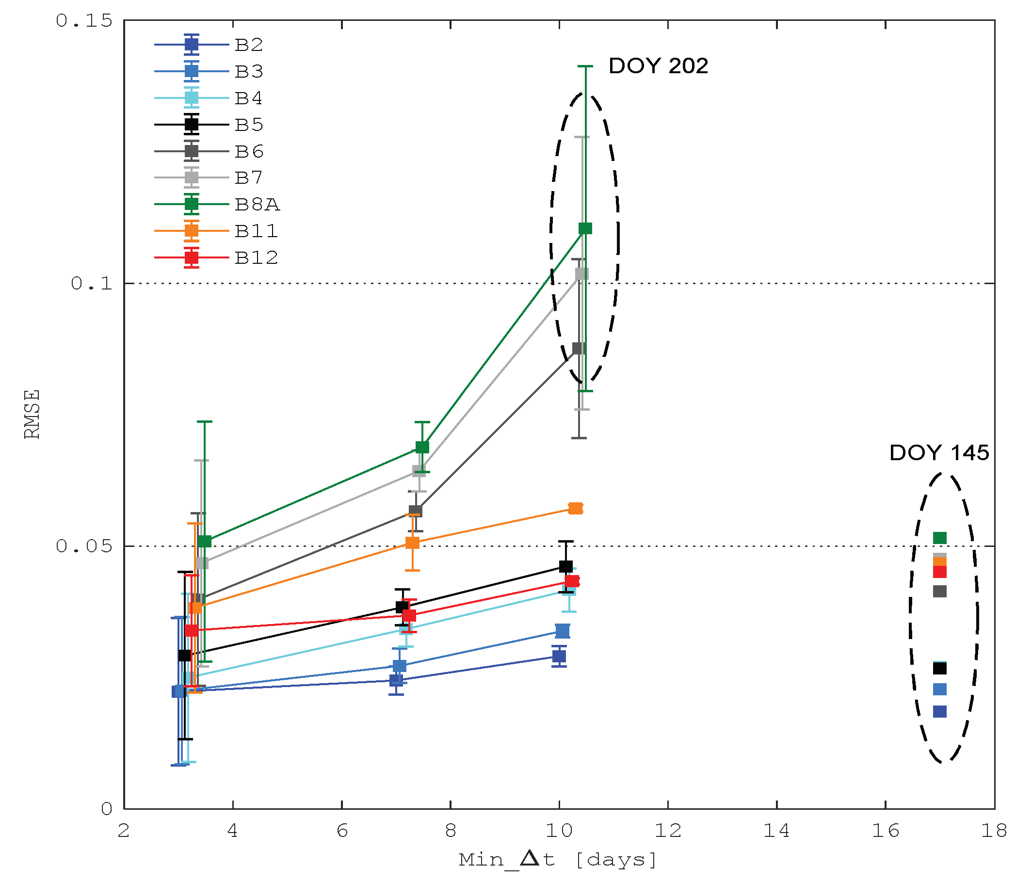
As shown in Figure 3, the uncertainty of S2-LIKE surface reflectance values generally increases as function of the temporal interval to the closest Start or End image (Min_), except for DOY 142. For DOY 142, low uncertainty (5%) was obtained despite the large temporal interval Min_ (17 days). The uncertainty of S2-LIKE surface reflectance products remains below 7% for other dates (Min_ ranges between 3 and 17 days), except for b6, b7, and b8A on DOY 202. Lower uncertainties are noted for b2, b3, and b4 (up to ~4%); slightly higher uncertainties are noted for b5, b11, and b12 (up to ~6%); and even higher for b6, b7, and b8A (up to ~14% for DOY 202). Visual assessment of input MSI imagery indicated that the DOY 202 the S2-MSI image had residual haze that may be the cause of the higher S2-LIKE reflectance uncertainties on this date.
4.2. Evaluation of Vegetation Biophysical Variables Estimated from Synthetic Images
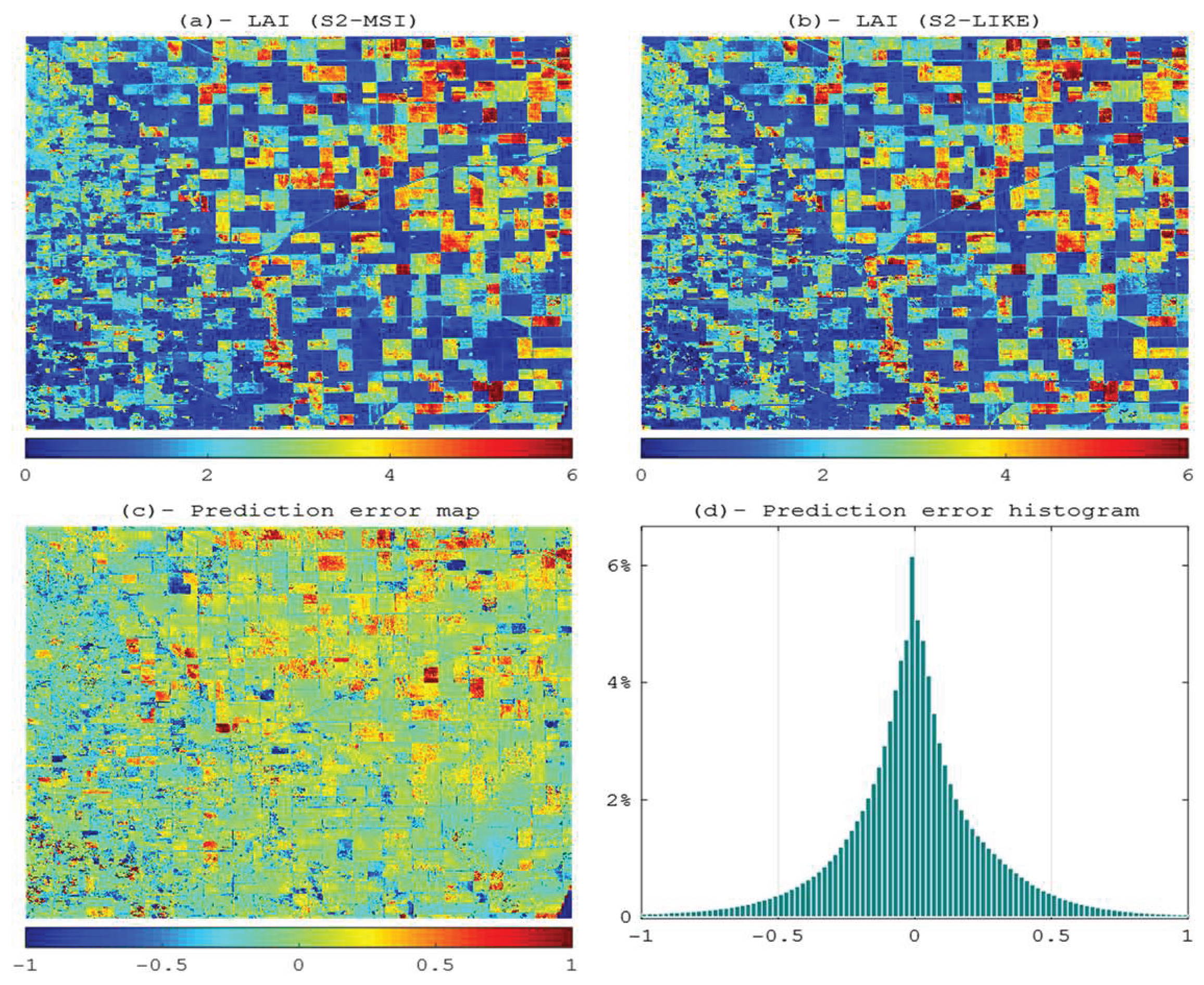
Differences between pairs of vegetation biophysical variables maps estimated using SL2P from S2-MSI and S2-LIKE images were qualitatively analyzed. Figure 4 shows an example of LAI maps derived on DOY175 and the corresponding prediction error map (the difference between LAI map derived from S2-MSI image and the corresponding map derived from S2-LIKE image) and histogram. Similarly, maps and histograms are generated and analyzed for other biophysical variables and dates (not shown). Generally, visual assessment indicated (1) high spatial correlation between biophysical variables maps (from 0.64 to 0.98, except for DOY 202) and (2) no particular spatial pattern of prediction error: higher prediction error was generally noted for high biophysical variable values (Figure 4a–c). Quantitatively, residuals indicated zero-centered Gaussian distributions for the prediction error for all the biophysical variables at all dates except for DOY 202 (e.g., Figure 4d).
Figure 5 presents density scatter plots between vegetation biophysical variables estimated using SL2P applied to S2-LIKE reflectance against the corresponding vegetation biophysical variables estimated using SL2P applied to S2-MSI reflectance on the same date. Estimates from all 13 acquisition dates (Table 2) were merged for the evaluation.
These graphs indicate that vegetation biophysical variables estimated from synthetic S2-LIKE images compared well to estimates from S2-MSI observations (slopes ranges from 0.85 to 0.94 for the different biophysical variables). The RMSE (bias) was equal to 0.55 (0.03) for LAI, 9.99% (1.59%) for FCOVER, 10.02% (−2.77%) for FAPAR, 0.13 g/m2 (0.17 g/m2) for CCC, and 0.16 kg/m2 (0.01 kg/m2) for CWC.
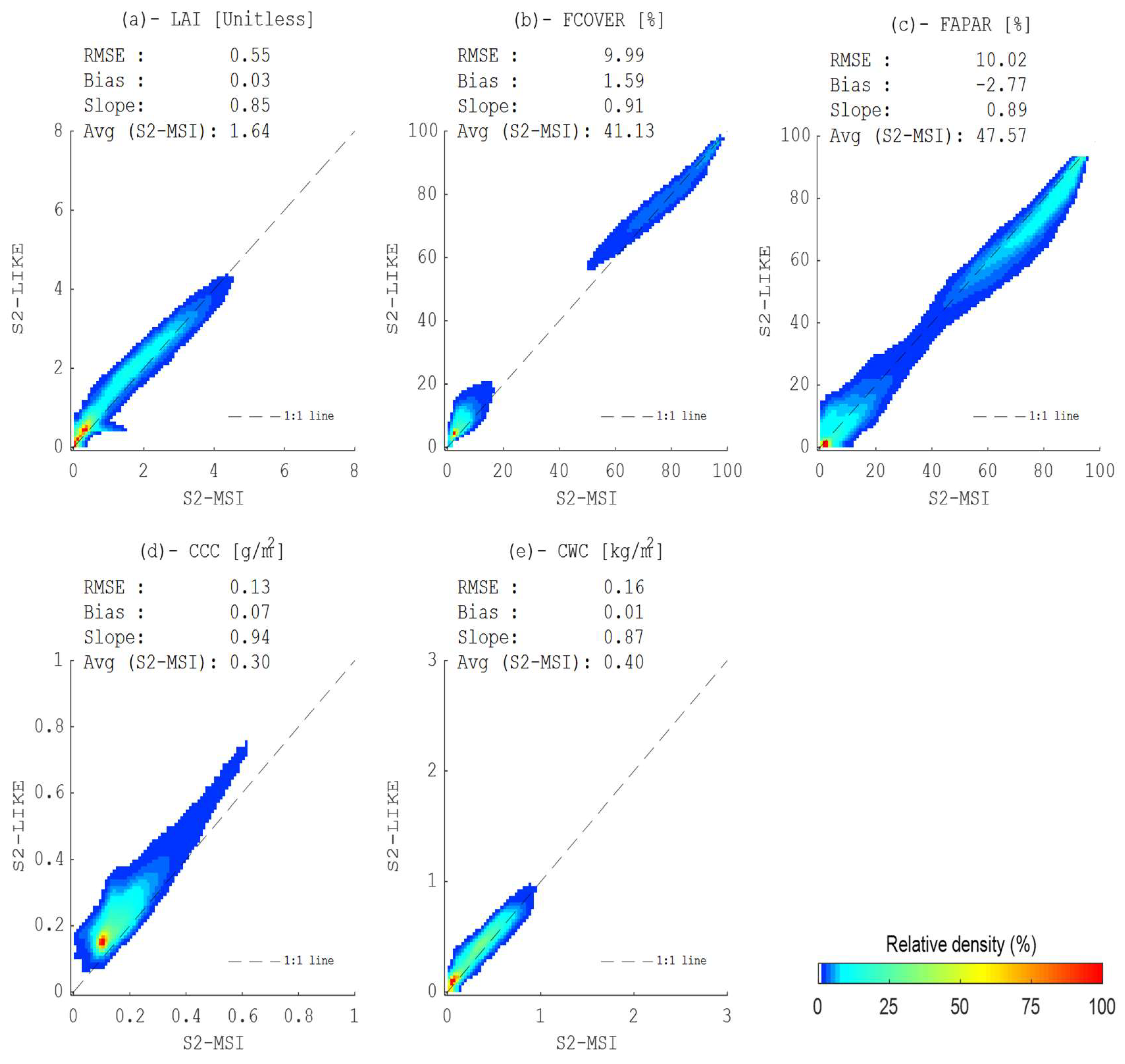
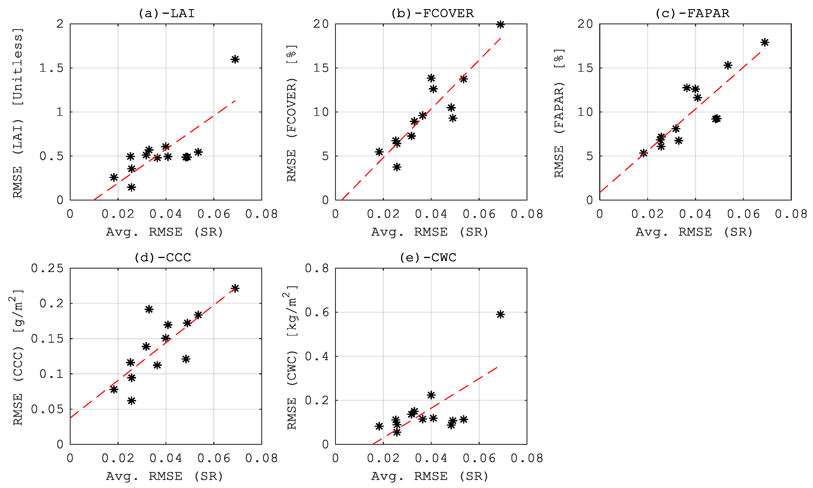
Figure 6 plots the RMSE values obtained between pairs of vegetation biophysical variables derived from S2-LIKE and S2-MSI images for the different prediction dates against RMSE values obtained between the corresponding pairs of surface reflectance datasets (average of RMSE values obtained from the different spectral bands for a given day). It indicates an increasing linear function between uncertainty of synthetic S2-LIKE surface reflectance data and uncertainty of corresponding estimated vegetation biophysical variables. An uncertainty of 0.02 (0.06) in terms of surface reflectance generates an uncertainty of ~0.25 (~0.6) LAI estimates, ~5% (~15%) on FCOVER and FAPAR estimates, ~0.06 g/m2 (~0.20 g/m2) on CCC estimates, and ~0.05 kg/m2 (~0.2 kg/m2) on CWC estimates.
4.3. Validation of Vegetation Biophysical Variables Estimated from Synthetic Images
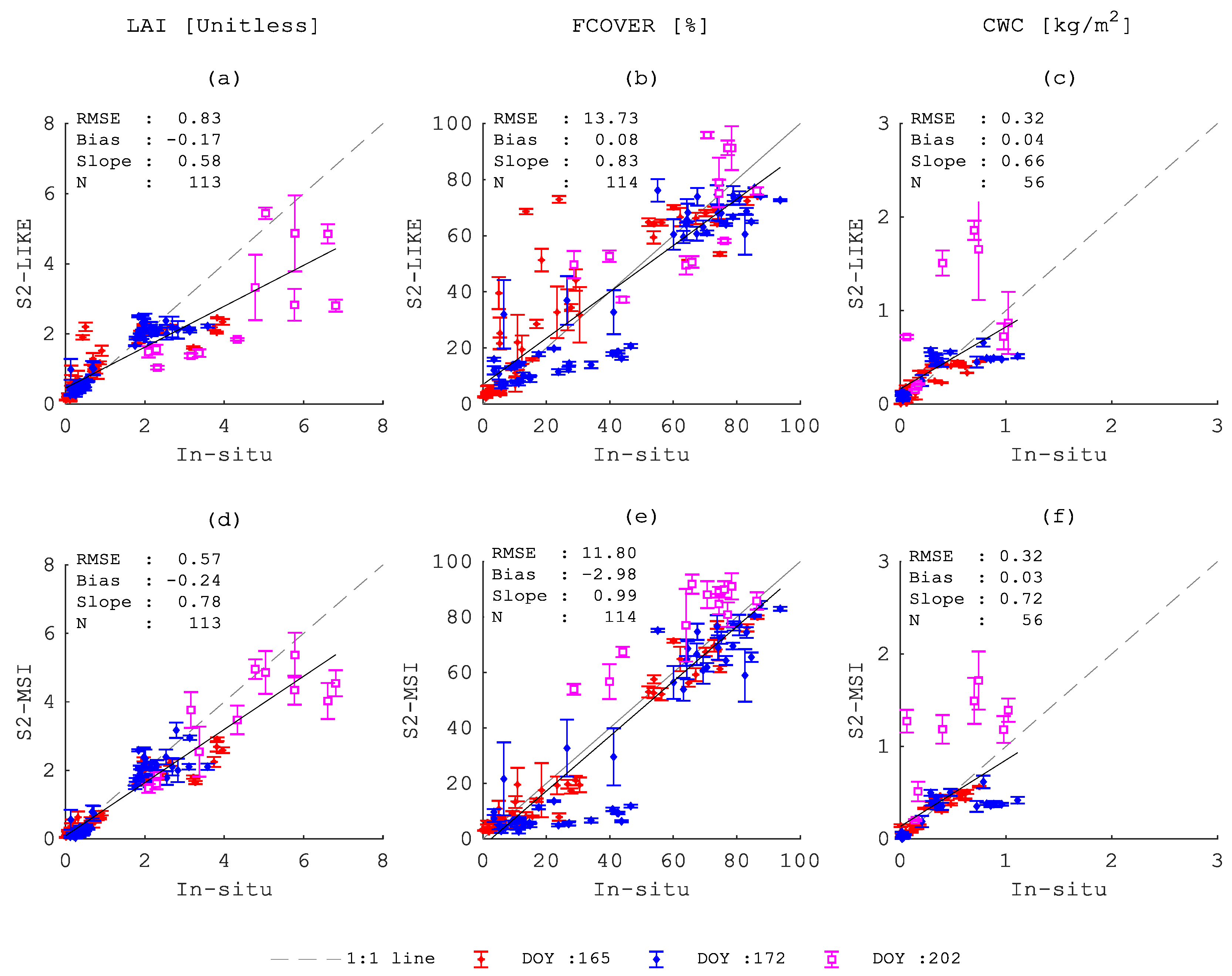
Figure 7 compares LAI, FCOVER and CWC estimated using SL2P applied to S2-LIKE (Figure 7a–c) and S2-MSI (Figure 7d–f) reflectance against in situ measurements. Validation statistics, computed from 113 samples for LAI, 114 samples for FCOVER and 56 samples for CWC, are provided, respectively.
Figure 7a indicates that LAI derived from S2-LIKE underestimates in situ data, as for estimates from S2-MSI (Figure 6d). Lower bias (−0.17) was obtained for LAI estimates from S2-LIKE by comparison to bias obtained for estimates from S2-MSI (−0.24). However, slope obtained for LAI estimates from S2-LIKE (0.58) is ~25% lower than slope obtained for LAI estimates from S2-MSI (0.78), and RMSE (0.83) was ~45% higher (RMSE = 0.57 for LAI estimates from S2-MSI).
For FCOVER, Figure 7b shows that estimates from S2-LIKE fit well with in situ data, particularly for DOY 172 and DOY 202. Low bias (0.08) was obtained between estimates and in situ data compared to bias obtained for estimates from S2-MSI (-2.98). Nevertheless, the slope (0.83) was ~15% lower than that from S2-LIKE (0.99), and the RMSE (13.73) is ~15% higher than RMSE obtained for estimates from S2-MSI (11.80).
For CWC, Figure 7c,f indicates that comparable statistics were obtained for estimates from S2-LIKE data (RMSE = 0.32; bias = 0.04; slope = 0.66) and estimates from S2-MSI (RMSE = 0.32; bias = 0.03; slope = 0.72). A wider scatter was noted for both datasets on DOY 202.
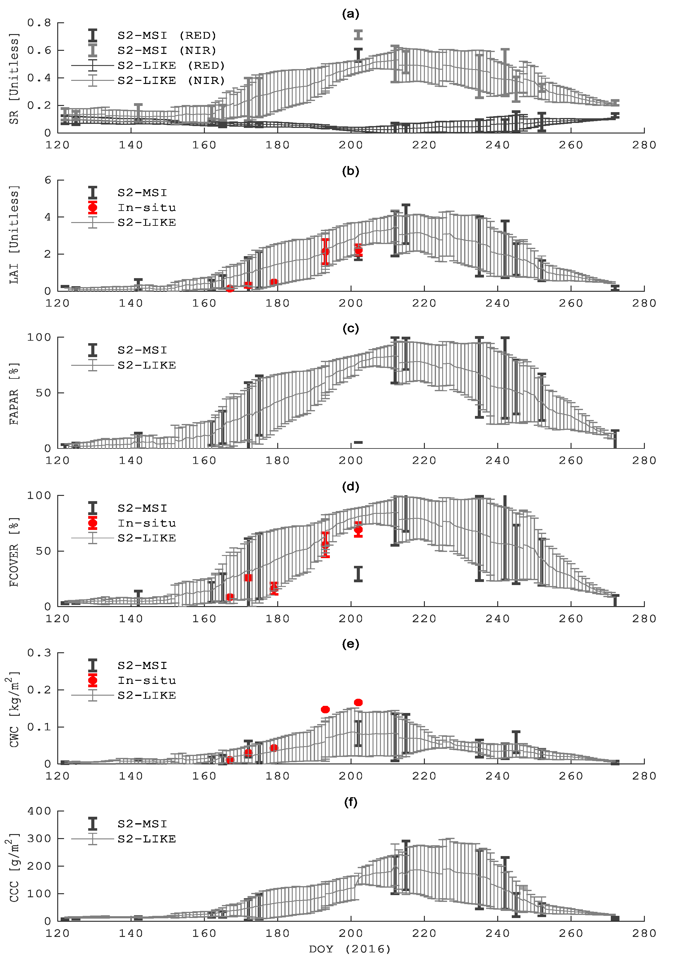
Figure 8a shows temporal profiles of surface reflectance data on RED and NIR bands from daily S2-LIKE and available S2-MSI images for one typical (soybean) field over the study area. Vertical bars present the one standard deviation interval of values computed from pixels included in the field. For the overlapping dates (e.g., from 125 to 142, Table 2), S2-LIKE estimates were selected from the closest preceding (i.e., 122–142) or following (i.e., 125–162) prediction model. Other bands or sites are not included for brevity. Figure 8f presents the corresponding temporal profiles of derived vegetation biophysical variables from S2-LIKE and S2-MSI images using SL2P. In situ measurements of LAI, FCOVER and CWC, are included in these figures.
Except for DOY 202, PSFRM predictions and derived S2-LIKE biophysical parameters closely match both the mean and standard deviation of observed MSI reflectance. The difference on DOY 202 was due to local haze contamination over the field as evidenced by the elevated S2-MSI red reflectance compared to S2-MSI retrievals before and after this date. It is noteworthy that PSFRM avoids this effect since it accounts for local residuals between the scene based calibration of reflectance changes and the S2-MSI reflectance change between calibration images. For this field, both S2-MSI and S2-LIKE systematically overestimated in situ LAI and FCOVER and overestimated in situ CWC. However, the temporal trends were nevertheless similar between S2-LIKE and in situ values and for LAI and FCOVER the in situ estimates were within the range of natural variability of the field.
5. Discussions
This research presents a first attempt at blending clear-sky S2-MSI and MODIS-NBAR images in order to produce time series of synthetic S2-LIKE products to supplement clear-sky S2-MSI images for applications, such as agricultural production monitoring, which require frequent medium spatial resolution surface reflectance images. S2-LIKE surface reflectance images and vegetation biophysical variables maps from the synthetic images were produced for 149 dates, and validated for thirteen (13) dates corresponding to the acquisition dates of the available S2-MSI images of the study area. These dates spanned rapid changes in surface conditions corresponding to the growth phase of all crops in the study area and offered both a realistic sampling of temporal gap sizes (from 10 to 40 days) and sufficient number of images for statistically reliable intercomparisons. Comparisons against in situ measurements were carried out for the three important stages for constraining crop productivity: DOY 165 (leaf emergence), 172 (vegetation growth), and DOY 202 (peak biomass). Ideally, additional comparisons during senescence/harvest and replicate sampling for each growth stage should be considered in further studies.
In terms of the estimation of surface reflectance, the typical error of between 2% to 6% across spectral bands is approximately twice than the end-to-end error estimate of 1–3% for surface reflectance over flat surfaces [42,43]. This is expected given the use of temporal interpolation and the additional uncertainty in the NBAR product. However, for the most part, the error still meets the 5% radiometric requirement for S2-MSI [44]. Similar uncertainties (RMSE 6%) were obtained when applying PSRFM on Landsat-8 images over an area dominated by cropland and forestland [20]. Improved haze screening and correction may further reduce the uncertainty in S2-LIKE reflectance estimates as this will improve the calibration of PSFRM.
Our study did not consider complex topography or pixels with shadows or water bodies. These targets may increase the uncertainty of PSFRM [20] since a linear prediction model as a function of land cover may no longer apply. However, we note that there is also substantial (>5%) uncertainty in current S2-MSI surface reflectance estimates based on the Sen2Cor algorithm over complex topography [39], so it may be premature to attempt to apply temporal interpolation over such areas until errors in the calibration S2-MSI images are understood and reduced.
Although the number of available dataset is limited for generalization, the estimation error of S2-LIKE reflectance showed an increasing function against to the time difference between the current date and the nearest calibration image (). For operational use, was expected to be relatively short due to (1) the use of all available S2A images (for this study S2A images are split into training and validation datasets) and the availability of S2B images (not available for this study). Consequently, we expect that the uncertainty of S2-LIKE surface reflectance data will further reduce if S2B-MSI data was also used as input.
The estimation error of S2-LIKE reflectance also varied with the presence of uncorrected atmospheric effects on S2-MSI images and the land cover. In fact, the low S2-LIKE surface reflectance uncertainty (RMSE 5%) obtained for DOY 145 with large (17 days) was explained by the low vegetation cover and the large uncertainty (RMSE up to 14%) obtained for DOY 202 with shorter (10 days) was explained by the haze observed within visible and near-infrared bands in the reference S2-MSI image. Residual atmospheric effects in S2-MSI surface reflectance data indicates issues with Sen2Cor atmospheric correction in the presence of haze. Similar issues were noted during systematic processing of Landsat Imager data and has led to the routine application of post-processing haze detection and removal algorithms [45]. The majority of haze removal algorithms rely on statistical multispectral relationships calibrated assuming a haze free set of pixels. In fact, if the calibration imagery is haze free and the interpolation duration short, PSFRM can be interpreted as an adaptive haze detection and removal. It would be interesting to compare PSFRM with other haze detection and removal algorithms.
Results confirmed that time series of vegetation biophysical variables (LAI, FCOVER, FAPAR, CCC, and CWC) could be estimated, with reasonable uncertainties and accuracies, from synthetic surface reflectance images predicted by blending clear-sky S2-MSI and MODIS-NBAR images (hypothesis 1). Vegetation biophysical variables maps derived from S2-LIKE surface reflectance images using SL2P compare well qualitatively and quantitatively with corresponding maps derived using SL2P with S2-MSI images. In addition to low biases between S2-LIKE and S2-MSI based products (2%, 4%, −6%, 23%, and 3% in comparison to the median values of LAI, FCOVER, FAPAR, CCC, and CWC, respectively), slopes between vegetation parameters maps (from 0.85 to 0.94) are closer to 1 than slopes obtained for surface reflectance datasets (from 0.65 to 0.85). In terms of uncertainty, the RMSE between estimates from S2-LIKE images and those from S2-MSI was 0.55 for LAI, ~10% for FCOVER and FAPAR, and 0.13 g/m2 for CCC and 0.16 kg/m2 for CWC. This uncertainty cannot be neglected as it is comparable to the performance requirement for LAI (20% or 1 unit) and FCOVER (15%) [2] and it is later reflected in increased uncertainty when comparing S2-LIKE based estimates with in situ data versus estimates derived using S2-MSI data directly. Nevertheless, the increase in error when using S2-LIKE data is almost linearly related to error in input reflectance indicating that uncertainty could potentially be modelled as a function of the temporal gap size. For our study, an uncertainty of ~2% (~6%) on S2-LIKE surface reflectance data (average value) produces an uncertainty of ~0.2 (~0.6) units on LAI estimation, ~5% (~15%) on FCOVER and FAPAR estimations, ~0.06 g/m2 (~0.20 g/m2) on CCC, and ~0.05 kg/m2 (~0.2 kg/m2) on CWC. These uncertainties may change with land surface condition and season so further studies should consider a systematic intercomparisons of products from interpolated and actual S2 imagery once larger datasets of products have been generated.
As expected, when compared to in situ measurements from SMAPVEX16, uncertainties of LAI and FCOVER estimates from S2-LIKE images were larger than uncertainties of LAI and FCOVER estimates from S2-MSI images (hypothesis 2). Although the difference between uncertainties was not significant for FCOVER (less than 2%), the uncertainty of LAI estimates from S2-LIKE images was ~45% higher than the uncertainty of LAI estimates from S2-MSI images. However, equal uncertainties (also accuracies) were obtained for CWC estimates from S2-LIKE and CWC estimates from S2-MSI images. This may reflect more on the low accuracy and uncertainty of SL2P for CWC estimation than the lack of sensitivity of SL2P to interpolation [11].
The scope of this study was limited to implementing and testing the intermediate and end-to-end performance of combining reflectance interpolation with a globally applicable algorithm for estimating multiple biophysical parameters simultaneously (SL2P). Future studies should compare this strategy with approaches that blend fine and coarse resolution parameter maps [24,25,26,27] although there is still the difficulty of specifying the error covariation matrix of these maps, especially in terms of validating coarse resolution product [46,47,48], required by both PSFRM and ESTARFM.
A complimentary approach to assessing the uncertainty of medium-resolution biophysical products derived from temporally interpolated reflectance data (e.g., S2-LIKE products) is to compare spatially upscaled versions of these products with products derived from high temporal frequency coarse resolution imagery (e.g., MODIS LAI, 42, 43, 44). Since the retrieval algorithms differ between products a local assessment of the uncertainty of the coarse resolution products that depends on either spatially extensive in situ sampling [49] or careful positioning of these samples to develop an upscaling transfer function [50]. We did not have sufficient sampling to implement this strategy. Future studies should consider more extensive in situ sampling designs to allow for comparisons between products derived from coarse resolution time series with fine resolution products derived using a different retrieval algorithm.
This study validated time series of vegetation biophysical variables derived from synthetic S2-LIKE surface reflectance data using SL2P processor. The model validation was pessimistic since S2B images were not included. Furthermore, the validation was performed over targets with a large change in vegetation variables. It would be useful to validate over targets with little or no change to evaluate the accuracy and the uncertainty of this algorithm. It would be also useful to validate over different ecosystems and topography complexities prior to application of this approach to larger extents. A third limitation of the actual study is the sensitivity of PSFRM to the clustering strategy used to stratify the calibration process. Here, we used a default set of clusters recommended by Zhong and Zhou [20]. However, there may be improvements if clustering is based perhaps of similarity of not just spectra but derived variables. Finally, since MODIS has a limited life time, work on using other coarse resolution sensors such as the Sentinel-3/Ocean and Land Color Imager (OLCI) and Sentinel-3/The Sea and Land Surface Temperature Radiometer (SLTR) or the Visible Infrared Imaging Radiometer should be considered assuming an NBAR equivalent product can be derived from these sensors.
6. Conclusions
The objectives of this research were to determine if subweekly vegetation biophysical parameter products can be derived using Sentinel 2 imagery and to validate these derived products. Results over our mid-latitude site showed that it is possible to use synthetic S2-LIKE surface reflectance data, produced by blending clear-sky S2-MSI images from Sentinel 2A with daily BRDF-adjusted MODIS images, to provide subweekly time series of vegetation biophysical variables at medium resolution (~20 m). Uncertainties of vegetation biophysical variables maps derived from synthetic surface reflectance data mainly depend on the temporal interval from the closest clear-sky S2-MSI image used for training. For temporal intervals ranging from 3 to 10 days, comparable uncertainties were obtained for CWC and FCOVER maps derived from S2-LIKE images and the corresponding maps derived from S2-MSI images. However, uncertainty of LAI maps from S2-LIKE images is ~45% larger than uncertainty of LAI maps from S2-MSI images. We hypothesize the addition of Sentinel 2B will decrease the uncertainty in reflectance estimates and subsequently the uncertainty in biophysical variable estimates due to a decrease in elapsed times between calibration dates and S2-LIKE image dates. This was the first study to perform end-to-end validation of multiple biophysical parameters and to confirm the relatively linear relationship between RMSE in predicted reflectance and RMSE of parameter estimates. While the study included a mixed land cover region specifically to pose a challenge to PSFRM it corresponds to a CEOS stage I validation [51] due to it being limited to a single growing season and location. Considering the relatively good end-to-end performance of the combination of PSFRM with the SEN2COR and SL2P processors and that all of these algorithms are globally applicable we recommend that this approach be tested over a broader range of conditions corresponding to CEOS stage II validation.
Author Contributions
Conceptualization and methodology, N.D. and R.F.; software, D.Z., F.Z. and N.D.; validation, N.D. and R.F.; formal analysis, N.D. and R.F.; investigation, N.D., R.F., D.Z. and F.Z.; data curation, N.D., D.Z.; writing—original draft preparation, N.D.; writing—review and editing, R.F., F.Z. and D.Z.
Funding
This research was funded by Natural Resources Canada (NRCan), Remote Sensing Science Program (RSSP), Canadian Space Agency (CSA) and Government Related Initiatives Program (GRIP).
Acknowledgments
The authors wish to acknowledge the Canadian Space Agency and Natural Resources Canada for supporting this work, the European Space Agency for the provision of Sentinel-2 data and Sen2Cor processor, United States Geological Survey for the provision of MODIS data and the French National Institute for Agricultural Research (INRA) for provision of SL2P processor. We also thank the external reviewers and the Editors for their comments on the manuscript.
Conflicts of Interest
The authors declare no conflict of interest.
References
- Food and Agriculture Organization of the United Nations. Terrestrial Essential Climate Variables for Climate Change Assessment, Mitigation and Adaptation. Biennial Report Supplement. 2008. Available online: www.fao.org/3/a-i0197e.pdf (accessed on 1 May 2019).
- Malenovsky, Z.; Rott, H.; Cihlar, J.; Schaepman, M.E.; Garcia-Santos, G.; Fernandes, R.; Berger, M. Sentinels for science: Potential of Sentinel-1, -2, and -3 missions for scientific observations of ocean, cryosphere. Remote Sens. Environ. 2012, 120, 91–101. [Google Scholar] [CrossRef]
- Global Climate Observing System. The Global Observing System for Climate: Implementation Needs. GCOS Steering Committee at Their 24th Meeting in Guayaquil. 2016. Available online: https://unfccc.int/sites/default/files/gcos_ip_10oct2016.pdf (accessed on 1 May 2019).
- European Space Agency. EO4SD-Earth Observation for Sustainable Development. Agriculture and Rural Development/Service Portfolio. 2019. Available online: https://www.eo4idi.eu/sites/default/files/eo4sd_agri_portfolio_170529_singlepag.pdf (accessed on 1 May 2019).
- Roy, D.P.; Yan, L. Robust landsat-based crop time series modelling. Remote Sens. Environ. 2018, 120, 91–101. [Google Scholar]
- The Committee on Earth Observation Satellites. The CEOS Database—Catalogue of Satellite Missions. 2019. Available online: http://database.eohandbook.com/ database/missiontable.aspx (accessed on 1 May 2019).
- Zhou, F.; Zhang, A. Methodology for estimating availability of cloud-free image composites: A case study for southern Canada. Int. J. Appl. Earth Obs. Geoinf. 2013, 21, 17–31. [Google Scholar] [CrossRef]
- Drusch, M.; Del Bello, U.; Carlier, S.; Colin, O.; Fernandez, V.; Gascon, F.; Hoersch, B.; Isola, C.; Laberinti, P.; Martimort, P.; et al. Sentinel-2: ESA’s optical high-resolution Mission for GMES operational services. Remote Sens. Environ. 2012, 20, 25–36. [Google Scholar] [CrossRef]
- Weiss, M.; Baret, F. S2ToolBox Level 2 Products, Version 1.1. 2016. Available online: Step.esa.int/docs/extra/ATBD_S2ToolBox_L2B_V1.1.pdf (accessed on 1 May 2019).
- Camacho, F.; Baret, F.; Weiss, M.; Fernandes, R.; Berthelot, B.; Sánchez, J.; Latorre, C.; García-Haro, J.; Duca, R. Validación de Algoritmos Para la Obtención de Variables Biofísicas con Datos Sentinel2 en la ESA: Proyecto VALSE-2. XV Congreso de la Asociación Española de Teledetección, INTA, Torrejón de Ardoz, Spain. 2013. Available online: https:// doi.org/10.13140/RG.2.1.4655.0241 (accessed on 1 May 2019).
- Djamai, N.; Fernandes, R.; Weiss, M.; McNairn, H.; Goita, K. Validation of the sentinel simplified level 2 product prototype processor (SL2P) for mapping cropland biophysical variables using Sentinel-2/MSI and Landsat-8/OLI data. Remote Sens. Environ. 2019, 225, 416–430. [Google Scholar] [CrossRef]
- Wulder, M.A.; Hilker, T.; White, J.C.; Coops, N.C.; Masek, J.G.; Pflugmacher, D.; Crevier, Y. Virtual constellations for global terrestrial monitoring. Remote Sens. Environ. 2015, 170, 62–76. [Google Scholar] [CrossRef] [Green Version]
- Claverie, M.; Junchang, J.; Masek, J.G.; Dungan, J.L.; Vermote, E.; Roger, J.L.; Skakun, S.V.; Justice, C. The harmonized Landsat and Sentinel-2 surface reflectance data set. Remote Sens. Environ. 2018, 219, 145–161. [Google Scholar] [CrossRef]
- Dorigo, W.A.; Zurita-Milla, R.; De Wit, A.J.W.; Brazile, J.; Singh, R.; Schaepman, M.E. A review on reflective remote sensing and data assimilation techniques for enhanced agroecosystem modeling. Int. J. Appl. Earth Obs. Geoinf. 2007, 9, 165–193. [Google Scholar] [CrossRef]
- Lauvernet, C.; Baret, F.; Hascoet, L.; Buis, S. Multitemporal-patch ensemble inversion of coupled surface-atmosphere radiative transfer models for land surface characterization. Remote Sens. Environ. 2008, 112, 851–861. [Google Scholar] [CrossRef]
- Hill, T.C.; Quaife, T.; Williams, M. A data assimilation method for using low-resolution Earth observation data in heterogeneous ecosystems. J. Geophys. Res. 2011, 116, D08117. [Google Scholar] [CrossRef]
- Pinty, B.; Lavergne, T.; Voßbeck, M.; Kaminski, T.; Aussedat, O.; Giering, R.; Gobron, N.; Taberner, M.; Verstraete, M.M.; Widlowski, J.L. Retrieving surface parameters for climate models from moderate resolution imaging spectroradiometer (MODIS)—Multiangle imaging spectroradiometer (MISR) albedo products. J. Geophys. Res. 2007, 112, D10116. [Google Scholar] [CrossRef]
- Ghamisi, P.; Rasti, B.; Yokoya, N.; Wang, Q.; Hofle, B.; Bruzzone, L.; Bovolo, F.; Chi, M.; Anders, K.; Gloaguen, R.; et al. Multisource and multitemporal data fusion in remote sensing: A comprehensive review of the state of the art. IEEE Geosci. Remote Sens. Mag. 2019, 7, 6–39. [Google Scholar] [CrossRef]
- Tian, Y.; Wang, Y.; Zhang, Y.; Knyazikhin, Y.; Bogaert, J.; Myneni, R.B. Radiative transfer based scaling of LAI retrievals from reflectance data of different resolutions. Remote Sens. Environ. 2003, 84, 143–159. [Google Scholar] [CrossRef]
- Zhong, D.; Zhou, F. A prediction smooth method for blending landsat and moderate resolution imagine spectroradiometer images. Remote Sens. 2018, 10, 1371. [Google Scholar] [CrossRef]
- Zhu, X.; Helmer, E.H.; Gao, F.; Liu, D.; Chen, J.; Lefsky, M.A. A flexible spatiotemporal method for fusing satellite images with different resolutions. Remote Sens. Environ. 2016, 172, 165–177. [Google Scholar] [CrossRef]
- Gao, F.; Masek, J.; Schwaller, M.; Hall, F. On the blending of the Landsat and MODIS surface reflectance: Predicting daily Landsat surface reflectance. IEEE Trans. Geosci. Remote Sens. 2006, 44, 2207–2218. [Google Scholar]
- Zhu, X.; Chen, J.; Gao, F.; Chen, X.; Masek, J.G. An enhanced spatial and temporal adaptive reflectance fusion model for complex heterogeneous regions. Remote Sens. Environ. 2010, 114, 2610–2623. [Google Scholar] [CrossRef]
- Houborg, R.; McCabe, M.F.; Gao, F. A spatio-temporal enhancement method for medium resolution LAI (STEM-LAI). Int. J. Appl. Earth Obs. Geoinf. 2016, 7, 15–29. [Google Scholar] [CrossRef]
- Yu, T.; Sun, R.; Xiao, Z.; Zhang, Q.; Wang, J.; Liu, G. Generation of high resolution vegetation productivity from a downscaling method. Remote Sens. 2018, 10, 1748. [Google Scholar] [CrossRef]
- Li, Z.; Huang, C.; Zhu, Z.; Gao, F.; Tang, H.; Xin, X.; Ding, L.; Shen, B.; Liu, J.; Chen, B.; et al. Mapping daily leaf area index at 30 m resolution over a meadow steppe area by fusing Landsat, Sentinel-2A and MODIS data. Int. J. Remote Sens. 2018, 39, 9025–9053. [Google Scholar] [CrossRef]
- Shang, J.; Liu, J.; Huffman, T.; Qian, B.; Pattey, E.; Wang, J.; Zhao, T.; Geng, X.; Kroetsch, D.; Dong, T.; et al. Estimation of crop leaf area index using Landsat-8 and Rapideye images. J. Appl. Remote Sens. 2014, 8, 085196. [Google Scholar] [CrossRef]
- Dong, T.; Liu, J.; Qian, B.; Zhao, T.; Jing, Q.; Geng, X.; Wang, J.; Huffman, T.; Shang, J. Estimating winter wheat biomass by assimilating leaf area index derived from fusion of Landsat-8 and MODIS data. Int. J. Appl. Earth. Obs. Geoinf. 2016, 49, 63–74. [Google Scholar] [CrossRef]
- Latifovic, R.; Pouliot, D.; Olthof, I. Circa 2010 land cover of canada: local optimization methodology and product development. Remote Sens. 2017, 9, 1098. [Google Scholar] [CrossRef]
- European Space Agency. Sentinel-2 Mission. Available online: https://sentinel.esa.int/web/sentinel/missions/sentinel-2 (accessed on 1 May 2019).
- Schaaf, C.B.; Gao, F.; Strahler, A.H.; Lucht, W.; Li, X.; Tsang, T.; Strugnell, N.C.; Zhang, X.; Jin, Y.; Muller, J.P.; et al. First operational BRDF, albedo nadir reflectance products from MODIS. Remote Sens. Environ. 2002, 83, 135–148. [Google Scholar] [CrossRef] [Green Version]
- The United States Geological Survey. Earth Explore Data Portal. Available online: https://earthexplorer.usgs.gov/ (accessed on 1 May 2019).
- Bhuiyan, H.A.K.M.; McNairn, H.; Powers, J.; Friesen, M.; Pacheco, A.; Jackson, T.J.; Cosh, M.H.; Colliander, A.; Berg, A.; Rowlandson, T.; et al. Assessing SMAP soil moisture scaling and retrieval in the Carman (Canada) study site. Vadose Zone J. 2018, 17, 180132. [Google Scholar] [CrossRef]
- McNairn, H.; Jackson, T.J.; Powers, J.; Bélair, S.; Berg, A.; Bullock, P.; Colliander, A.; Cosh, M.H.; Kim, S.B.; Magagi, R.; et al. SMAPVEX16 Database Report. 2017. Available online: http://smapvex16-mb.espaceweb.usherbrooke.ca/documents/SMAPVEX16-MB_Experimental_Plan.pdf (accessed on 1 May 2019).
- Fernandes, R. Canada Centre for Remote Sensing Protocol for In-Situ Leaf Area Index Using Digital Hemispherical Photography Using the INRA CANEYE. Analysis Systemi; Canada Centre for Remote Sensing Report Series: Ottawa, ON, Canada, 2019. [Google Scholar]
- European Space Agency. The Sentinel Application Platform (SNAP). Available online: http://step.esa.int/main/toolboxes/snap/ (accessed on 1 May 2019).
- Mueller-Wilm, U.; Devignot, O.; Pessiot, L. Sen2Cor Configuration and User Manual. S2-PDGS-MPC-L2A-SUM-V2.4. 2017. Available online: http://step.esa.int/thirdparties/sen2cor/2.4.0/Sen2Cor_240_Documenation_PDF/S2-PDGS-MPC-L2A-SUM-V2.4.0.pdf (accessed on 1 May 2019).
- The EOSDIS Distributed Active Archive Centers. The MODIS Projection Tool 3.3. Available online: https://earthdata.nasa.gov/earth-observation-data/tools/ (accessed on 1 May 2019).
- Wolf, P.R. Survey Measurement Adjustments by Least Squares. In The Surveying Handbook; Springer: Boston, MA, USA, 1995; pp. 383–413. [Google Scholar]
- Jacquemoud, S.; Baret, F. PROSPECT: A model of leaf optical properties spectra. Remote Sens. Environ. 1990, 34, 75–91. [Google Scholar] [CrossRef]
- Verhoef, W. Light scattering by leaf layers with application to canopy reflectance modeling: The SAIL model. Remote Sens. Environ. 1984, 16, 125–141. [Google Scholar] [CrossRef] [Green Version]
- Doxani, G.; Vermote, E.; Roger, J.C.; Gascon, F.; Adriaensen, S.; Frantz, D.; Hagolle, O.; Hollstein, A.; Kirches, G.; Li, F.; et al. Atmospheric correction inter-comparison exercise. Remote Sens. 2018, 10, 352. [Google Scholar] [CrossRef]
- Djamai, N.; Fernandes, R. Comparison of SNAP-derived sentinel-2A L2A product to ESA product over Europe. Remote Sens. 2018, 10, 926. [Google Scholar] [CrossRef]
- ESA Sentinel-2 Team. GMES Sentinel-2 Mission Requirements Document. EOP-SM/1163/MR-dr. Available online: https://earth.esa.int/pub/ESA_DOC/GMES_Sentinel2_MRD_issue_2.0_update.pdf (accessed on 1 May 2019).
- Ju, J.; Roy, D.P.; Vermote, E.; Masek, J.G.; Kovalskyy, V. Continental-scale validation of MODIS-based and LEDAPS Landsat ETM+ atmospheric correction methods. Remote Sens. Environ. 2012, 122, 175–184. [Google Scholar] [CrossRef] [Green Version]
- Xiao, Z.; Liang, S.; Wang, J.; Chen, P.; Yin, X.; Zhang, L.; Song, J. Use of general regression neural networks for generating the GLASS leaf area index product from time-series MODIS surface reflectance. IEEE Trans. Geosci. Remote Sens. 2014, 52, 209–223. [Google Scholar] [CrossRef]
- Yan, K.; Park, T.; Yan, G.; Chen, C.; Yang, B.; Liu, Z.; Nemani, R.; Knyazikhin, Y.; Myneni, R. Evaluation of MODIS LAI/FPAR product Collection 6. Part 1: Consistency and improvements. Remote Sens. 2016, 8, 359. [Google Scholar] [CrossRef]
- Baret, F.; Weiss, M.; Lacaze, R.; Camacho, F.; Makhmara, H.; Pacholcyzk, P.; Smets, B. GEOV1: LAI and FAPAR essential climate variables and FCOVER global time series capitalizing over existing products. Part1: Principles of development and production. Remote Sens. Environ. 2013, 137, 299–309. [Google Scholar] [CrossRef]
- Canisius, F.; Fernandes, R.; Chen, J. Comparison and evaluation of medium resolution imaging spectrometer leaf area index products across a range of land use. Remote Sens. Environ. 2010, 114, 950–960. [Google Scholar] [CrossRef]
- Fernandes, R.; Plummer, S.; Nightingale, J. Global Leaf Area Index Product Validation Good Practices. Committee of Earth Observing Systems Working Group on Calibration and Validation; CEOS: Rome, Italy, 2014; p. 75. [Google Scholar]
- CEOS Working Group on Calibration and Validation. Land Product Validation Subgroup. Available online: https://lpvs.gsfc.nasa.gov/ (accessed on 10 June 2019).
Figure 1.
Study site and sampled fields (Basemap: Land Cover of Canada [29]).
Figure 1.
Study site and sampled fields (Basemap: Land Cover of Canada [29]).

Figure 2.
Surface reflectance data from S2-LIKE product compared to the corresponding surface reflectance data from S2-MSI product (# ~11 × 107 samples).
Figure 2.
Surface reflectance data from S2-LIKE product compared to the corresponding surface reflectance data from S2-MSI product (# ~11 × 107 samples).

Figure 3.
RMSE between surface reflectance datasets from S2-LIKE and S2-MSI as function of the temporal interval to clear-sky S2-MSI image used for training (): points (error bars) present the mean (standard deviation) of RMSE values obtained for spectral band predictions with equal .
Figure 3.
RMSE between surface reflectance datasets from S2-LIKE and S2-MSI as function of the temporal interval to clear-sky S2-MSI image used for training (): points (error bars) present the mean (standard deviation) of RMSE values obtained for spectral band predictions with equal .

Figure 4.
Example of LAI maps derived from S2-MSI (a) and S2-LIKE (b) images on DOY 175 (b), as well as the corresponding LAI prediction error map (c) and histogram (d).
Figure 4.
Example of LAI maps derived from S2-MSI (a) and S2-LIKE (b) images on DOY 175 (b), as well as the corresponding LAI prediction error map (c) and histogram (d).

Figure 5.
Vegetation biophysical variables derived from S2-LIKE product compared to the corresponding vegetation biophysical variables derived from S2-MSI (# ~11 × 107 samples).
Figure 5.
Vegetation biophysical variables derived from S2-LIKE product compared to the corresponding vegetation biophysical variables derived from S2-MSI (# ~11 × 107 samples).

Figure 6.
RMSE between pairs of vegetation biophysical variables derived from S2-LIKE and S2-MSI against the average of RMSE values obtained from the different spectral bands for the corresponding surface reflectance datasets.
Figure 6.
RMSE between pairs of vegetation biophysical variables derived from S2-LIKE and S2-MSI against the average of RMSE values obtained from the different spectral bands for the corresponding surface reflectance datasets.

Figure 7.
Vegetation biophysical variables derived using SL2P from S2-LIKE (top) and S2-MSI (bottom) images compared to in situ data.
Figure 7.
Vegetation biophysical variables derived using SL2P from S2-LIKE (top) and S2-MSI (bottom) images compared to in situ data.

Figure 8.
Time series of (a) surface reflectance (SR) data (RED and NIR bands), (b) LAI, (c) FAPAR, (d) FCOVER, (e) CWC, and (f) CCC from S2-LIKE images, S2-MSI images, and in situ measurements (for LAI, FCOVER, and CWC).
Figure 8.
Time series of (a) surface reflectance (SR) data (RED and NIR bands), (b) LAI, (c) FAPAR, (d) FCOVER, (e) CWC, and (f) CCC from S2-LIKE images, S2-MSI images, and in situ measurements (for LAI, FCOVER, and CWC).


Table 1.
Sentinel-2 Multispectral Imager (S2-MSI) bands used by SL2P and the corresponding Moderate Resolution Imaging Spectroradiometer (MODIS) bands.
Table 1.
Sentinel-2 Multispectral Imager (S2-MSI) bands used by SL2P and the corresponding Moderate Resolution Imaging Spectroradiometer (MODIS) bands.
| S2-MSI | MODIS | |||||
|---|---|---|---|---|---|---|
| Band Name | Band ID | Bandwidth (nm) | Spatial Resolution (m) | Band ID | Bandwidth (nm) | Spatial Resolution (m) |
| Blue | b2 | 439–533 | 10 | b3 | 459–479 | 500 |
| Green | b3 | 538–583 | 10 | b4 | 545–565 | 500 |
| Red | b4 | 646–684 | 10 | b1 | 620–670 | 500 |
| Red-edge 1 | b5 | 695–714 | 20 | - | - | |
| Red-edge 2 | b6 | 731–749 | 20 | - | - | |
| Red-edge 3 | b7 | 769–797 | 20 | - | - | |
| Near-Infrared (NIR) | b8A | 837–881 | 20 | b2 | 841–876 | 500 |
| Shortwave Infrared (SWR1) | b11 | 1539–1682 | 20 | b6 | 1628–1652 | 500 |
| Shortwave Infrared (SWR2) | b12 | 2078–2320 | 20 | b7 | 2105–2155 | 500 |
Table 2.
Day-of-year (DOY) of available S2-MSI images (% of cloud cover), synthetized S2-LIKE images (the corresponding subperiod start–end dates) and in situ measurements, as well as the temporal interval (Min_T) between DOY of S2-LIKE images and the closest start or end date of the corresponding subperiod period.
| DOY | S2-MSI (Cloud Cover %) | S2-LIKE (Start–End Dates) | T [Days] | In situ Data |
|---|---|---|---|---|
| 122 | ~1% | - | - | |
| 125 | ~1% | 122–142 | 3 | |
| 142 | ~2% | 125–162 | 17 | |
| 162 | ~1% | 142–165 | 3 | |
| 165 | ~1% | 162–172 | 3 | x |
| 172 | ~1% | 165–175 | 3 | x |
| 175 | ~1% | 172–212 | 3 | |
| 202 | ~66% | 175–212 | 10 | x |
| 212 | ~2% | 175–215 | 3 | |
| 215 | ~1% | 212–235 | 3 | |
| 235 | ~1% | 215–242 | 7 | |
| 242 | ~4% | 235–252 | 7 | |
| 245 | ~11% | 242–252 | 3 | |
| 252 | ~0% | 242–272 | 10 | |
| 272 | ~4% | - | - | - |
© 2019 by the authors. Licensee MDPI, Basel, Switzerland. This article is an open access article distributed under the terms and conditions of the Creative Commons Attribution (CC BY) license (http://creativecommons.org/licenses/by/4.0/).
Share and Cite
MDPI and ACS Style
Djamai, N.; Zhong, D.; Fernandes, R.; Zhou, F. Evaluation of Vegetation Biophysical Variables Time Series Derived from Synthetic Sentinel-2 Images. Remote Sens. 2019, 11, 1547. https://0-doi-org.brum.beds.ac.uk/10.3390/rs11131547
AMA Style
Djamai N, Zhong D, Fernandes R, Zhou F. Evaluation of Vegetation Biophysical Variables Time Series Derived from Synthetic Sentinel-2 Images. Remote Sensing. 2019; 11(13):1547. https://0-doi-org.brum.beds.ac.uk/10.3390/rs11131547
Chicago/Turabian StyleDjamai, Najib, Detang Zhong, Richard Fernandes, and Fuqun Zhou. 2019. "Evaluation of Vegetation Biophysical Variables Time Series Derived from Synthetic Sentinel-2 Images" Remote Sensing 11, no. 13: 1547. https://0-doi-org.brum.beds.ac.uk/10.3390/rs11131547
Note that from the first issue of 2016, this journal uses article numbers instead of page numbers. See further details here.