Article

Mid-season Crop Classification Using Dual-, Compact-, and Full-Polarization in Preparation for the Radarsat Constellation Mission (RCM)

1
C-CORE and Department of Electrical and Computer Engineering, Memorial University of Newfoundland, St. John’s, NL A1B 3X5, Canada
2
Ottawa Research and Development Centre, Agriculture and Agri-Food Canada, Ottawa, ON K1A 0C6, Canada
3
CRC-Laboratory in Advanced Geomatics Image Processing, Department of Geodesy and Geomatics Engineering, University of New Brunswick, Fredericton, NB NB E3B 5A3, Canada
4
Environmental Resources Engineering, College of Environmental Science and Forestry, State University of New York, NY 13210, USA
5
Centre Eau Terre Environnement, Institut National de la Recherche Scientifique, Québec, QC G1K 9A9, Canada
*
Author to whom correspondence should be addressed.
Remote Sens. 2019, 11(13), 1582; https://0-doi-org.brum.beds.ac.uk/10.3390/rs11131582
Submission received: 19 May 2019 / Revised: 25 June 2019 / Accepted: 26 June 2019 / Published: 3 July 2019
(This article belongs to the Special Issue Compact Polarimetric SAR)

Abstract

:
Despite recent research on the potential of dual- (DP) and full-polarimetry (FP) Synthetic Aperture Radar (SAR) data for crop mapping, the capability of compact polarimetry (CP) SAR data has not yet been thoroughly investigated. This is of particular concern, given the availability of such data from RADARSAT Constellation Mission (RCM) shortly. Previous studies have illustrated potential for accurate crop mapping using DP and FP SAR features, yet what contribution each feature makes to the model accuracy is not well investigated. Accordingly, this study examined the potential of the early- to mid-season (i.e., May to July) RADARSAT-2 SAR images for crop mapping in an agricultural region in Manitoba, Canada. Various classification scenarios were defined based on the extracted features from FP SAR data, as well as simulated DP and CP SAR data at two different noise floors. Both overall and individual class accuracies were compared for multi-temporal, multi-polarization SAR data using the pixel- and object-based random forest (RF) classification schemes. The late July C-band SAR observation was the most useful data for crop mapping, but the accuracy of single-date image classification was insufficient. Polarimetric decomposition features extracted from CP and FP SAR data produced relatively equal or slightly better classification accuracies compared to the SAR backscattering intensity features. The RF variable importance analysis revealed features that were sensitive to depolarization due to the volume scattering are the most important FP and CP SAR data. Synergistic use of all features resulted in a marginal improvement in overall classification accuracies, given that several extracted features were highly correlated. A reduction of highly correlated features based on integrating the Spearman correlation coefficient and the RF variable importance analyses boosted the accuracy of crop classification. In particular, overall accuracies of 88.23%, 82.12%, and 77.35% were achieved using the optimized features of FP, CP, and DP SAR data, respectively, using the object-based RF algorithm.

Graphical Abstract

1. Introduction

Over the past 15 years, the Government of Canada—led by Agriculture and Agri-Food Canada, the Federal department responsible for Canada’s agriculture sector—has devoted considerable effort to better understanding how Earth Observation (EO) technologies can be used to operationally provide timely and repeatable observations of Canadian agriculture at a national scale. Accordingly, many studies have highlighted the utility of using spectral vegetation indices (VIs) derived from optical observations (particularly, R, NIR and SWIR) for use in agricultural applications [1,2]. However, the application of optical remote sensing is limited by its restriction to daytime monitoring through cloud-free skies [3]. This is of particular concern for the systematic operational monitoring of agricultural regions that experience frequent cloud cover, such as Canada’s east and west coasts. In contrast, Synthetic Aperture Radar (SAR) sensors have the ability to penetrate clouds, smoke, haze and darkness, thus providing all-weather day-and-night imaging capability. This flexibility makes SAR a popular choice of national monitoring agencies for the operational monitoring of land, coastal and ocean environments.
The ability of SAR to distinguish between crop classes depends on the exact nature of the SAR sensor itself. As a general rule, single-polarized (SP) SAR is less useful to discriminate among crop types compared to dual-polarized (DP) SAR which, in turn, is generally less useful to discriminate among crop types compared to full polarimetric (FP) SAR. FP SAR is the most useful of these modes because FP SARs collect the full suite of possible horizontal and vertical polarizations which better allows for the discrimination of crop types with similar structures. FP SAR sensors transmit a fully polarized signal toward the ground target and receive a backscattering response that contains both fully polarized and depolarized constituents [4]. These sensors collect data at four polarization channels, which comprise the full scattering matrix for each ground resolution cell [5]. In addition, the relative phase between polarization channels is maintained that allows SAR backscattering responses to be decomposed into various scattering mechanisms using advanced polarimetric decomposition techniques [6]. These techniques allow the polarimetric covariance or coherency matrixes to be decomposed into three main scattering mechanisms: (1) single/odd-bounce scattering, which represents a direct scattering from the vegetation or ground surface; (2) double/even-bounce scattering, which represents a scattering between, for example, a plant stalk and the ground surface; and (3) volume scattering, which represents multiple scattering within the developed vegetation canopies [7,8].
Despite promising results having been obtained from FP SAR data for land cover classification in a variety of applications to date [7,8], it is limited from an operational perspective for two main reasons. First, there is an inherent time constraint associated with the alternating transmission of H- and V-polarized pulses [9]. Second, the complexity due to the double pulse repetition frequency and an increase in data rate relative to SP SAR systems [10], halves the image swath width of FP SAR systems, decreasing satellite coverage and increasing revisit times. This hinders the utility of FP SAR for operational applications that demand data over large geographical extents. While DP SAR partially addresses some of these limitations (e.g., small swath width), its inability to maintain relative phase between co- and cross-polarization channels remains a problem [9].
A solution to the previously described limitations of the DP and FP SAR configurations may lie in the use of compact polarimetry (CP) SAR [11]. Over the past few years, CP SAR observations (e.g., from RISAT-1 and ALOS PALSAR-2) and simulated CP observations have drawn attention within the radar remote sensing community. Similar to DP SAR, a CP sensor transmits one polarization and receives two coherent polarizations simultaneously, thus alleviating the inherent time constraint attributed to that of FP SAR sensors. These sensors collect more scattering information than SP and DP SAR sensors, and are comparable to that obtained from FP systems at a swath width two times larger than FP sensors. Moreover, the relative phase between polarization channels can be maintained using this configuration [12].
There are three CP SAR configurations in the context of EO sensors. These modes are: (1) π / 4 [12], (2) circularly transmitting circularly receiving (CC; [5,13]), and (3) circularly transmitting linearly receiving (CTLR; [14]). The third configuration is of particular interest in a Canadian context because of its use in the RADARSAT Constellation Mission (RCM). A CTLR SAR sensor transmits either right or left circular polarization and receives both linear polarizations (H and V) coherently.
The RCM contains three identical C-band SAR satellites, which improve satellite revisit time [15]. The primary purposes of the RCM mission are to ensure data continuity for RADARSAT users and improve operational capability by collecting sub-weekly data (i.e., a four day repeat cycle) for a variety of applications, including maritime surveillance, disaster management, and ecosystem monitoring [16]. Various polarization settings, including SP (i.e., HH, VV, and HV or VH), DP (i.e., HH-HV, VV-VH, and HH-VV), and CP (i.e., CTLR) modes, at varying spatial resolutions and noise floors, are available with RCM. One major drawback, however, is the higher noise equivalent sigma zero (NESZ) of RCM compared to RADARSAT-2. In particular, NESZ values can vary between −25 to −17 dB for RCM data [16], resulting in a decreased sensitivity to low backscattering values within a SAR image.
Previous studies found that cross-polarized SAR data (VH or HV) are the most useful SAR observations for crop mapping, though the inclusion of the second polarization (VV) can significantly increase classification accuracy [17,18]. For example, AAFC’s Annual Space-Based Crop Inventory uses DP SAR data (VV/VH from RADARSAT-2) along with optical observations to produce overall accuracies of 85% and above [19]. The addition of the third polarization; however, may improve the accuracies of some crop classes [18]. Although previous research has examined several aspects of SAR data, including the most useful wavelengths and polarizations, fewer investigations have been carried out to identify the most effective polarimetric decomposition features for accurate crop mapping using either FP or CP SAR data [3]. For example, McNairn et al. (2009b) reported the superiority of decomposition features, such as Cloude-Pottier and Freeman-Durden, compared to the intensity channels for crop classification using ALOS PALSAR L-band data [18]. Charbonneau et al. (2010) also noted that the Stokes parameters extracted from simulated CP data were useful for crop classification [12]. Nonetheless, no comprehensive examination of polarimetric decomposition parameters extracted from FP and CP SAR data for accurate crop mapping exists [3].
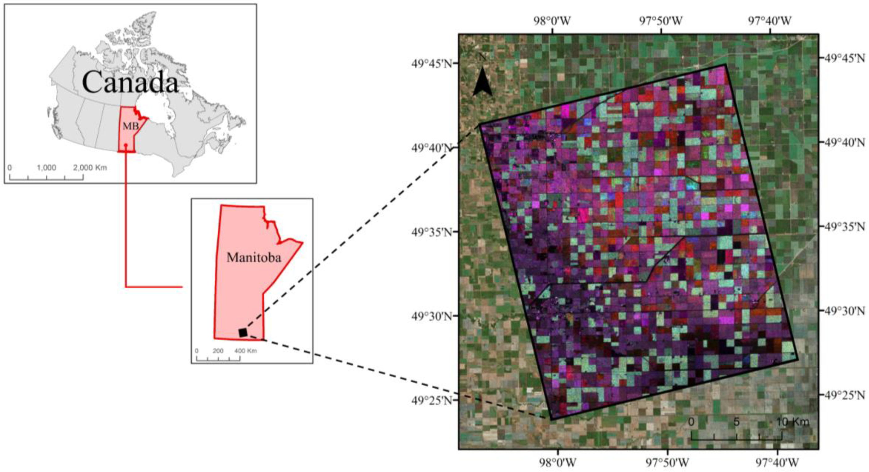
In this study, we undertake a much-needed investigation to identify the potential of polarimetric decomposition features extracted from FP RADARSAT-2 data and simulated CP data collected over an agricultural region near Winnipeg, Manitoba, Canada. In particular, the main purposes of this research are to:
(1)
confirm the necessity of multi-temporal SAR observations for capturing phenological information of cropping systems;
(2)
investigate the effect of the difference in polarization between FP (RADARSAT-2) and simulated HH/HV, VV/VH, and CP SAR data (to be collected by RCM) for complex crop classification;
(3)
examine the effects of difference in radiometry by simulating CP data at two NESZ of −19 dB and −24 dB for crop mapping;
(4)
identify the most useful polarimetric decomposition features that can be extracted from FP and CP SAR data; and
(5)
determine the ability of early- and mid-season PolSAR observations for crop classification.
The results of this study will advance our understanding of the use of CP SAR data to be collected by RCM for operational crop mapping prior to the availability of such an important EO data.

2. Study Area and Dataset

The study area is an agricultural area located in the Red River Watershed, Manitoba, Canada (Figure 1). Southern Manitoba is characterized by a typical sub-humid to a humid continental climate, and experiences temperature variations between −30 °C and 30 °C [20]. The same study location was used for the Soil Moisture Active Passive Validation Experiment (SMAPVEX12), carried out in support of the calibration/validation campaign of NASA’s Soil Moisture Active-Passive satellite (SMAP) in 2012 [21]. The study area is characterized by mixed prairies, cereals, soybeans, canola and corn. During the SMAPVEX12 field campaign, a total of 55 annual and perennial crop fields were visited between June 7, 2012 (early crop development) and July 19, 2012 (maximum crop biomass). Surface soil moisture and crop biophysical information (e.g., structure, biomass, water content and leaf area index (LAI)) were collected within each field at this time. This in situ data collection strategy was timed to capture soil- and crop-related information during the most crucial crop developmental stages. A more detailed description of this field campaign is presented in [21]. Table 1 outlines the independent training and testing samples for the six crop types analyzed in this study.
During the SMAPVEX12 campaign, Wide Fine Quad (FQW) polarimetric C-band RADARSAT-2 data were acquired. Four Single Look Complex (SLC) RADARSAT-2 images, acquired on May 10, June 3, June 27, and July 21 (exact 24-day repeat), were used in this study. These images were selected because their dates of acquisition best corresponded to those required for estimating early- and mid-season (before August) acreage yields. All images were acquired in an ascending orbit with the same geometry (Fine Wide Quad pol 2 (FQ2W) with a center incidence angle of ~20° and a ground range resolution of ~16 m). This eliminated the influences of other factors such as variances in incidence angles, which affect the backscattering responses of differing crops. The Canada Centre for Mapping and Earth Observation (CCMEO) simulator was employed to simulate data at various polarizations and noise floors [12]. In particular, the SLC RADARSAT-2 data were incorporated into the CCMEO software, and DP (i.e., HH/HV and VV/VH) and CP SAR data were simulated at both −19 and −24 dB NESZ.

3. Methods

3.1. Preprocessing

Speckle reduction, orthorectification, and image mosaicking were the main SAR preprocessing steps employed in this study. The presence of speckle noise affects the radiometric quality of PolSAR data and its subsequent image processing [22]. A Boxcar filter with a 5 × 5 kernel size was used to suppress the effect of speckle noise and increase the number of looks before the extraction of polarimetric features. A Boxcar filter was used because it was the only available speckle filter within the CCMEO simulator at the time of data processing in this study. The selected small size filter (5 × 5) was the most appropriate for the sizes of field in the study area and minimized the cross-boundary averaging of features belonging to different land cover classes. The de-speckled images preserved the mean brightness values, while maintaining image detail and reducing the standard deviation of non-homogeneous regions. Processing SAR data with other geo-data products, such as in situ data, requires the transformation from radar (slant-range) geometry to conventional map (ground-range) geometry. In this study, RADARSAT-2 level-1 SLC was orthorectified with PCI Geomatica’s OrthoEngine 2017 software using the rational function model. An external digital elevation model (DEM), released by Natural Resource Canada at the scale of 1:50,000, as well as satellite orbital information, were used during orthorectification. All images were projected to UTM coordinates (zone 14, northern hemisphere) using the NAD83 reference ellipsoid. Three orthorectified RADARSAT-2 images in a single orbit, collected on the same day, were mosaicked to cover the surveyed area during the SMAPVEX12 campaign.

3.2. Feature Extraction

3.2.1. Full Polarimetric SAR Data

SAR backscattering coefficient images are essential features for crop mapping. This is because intensity features are highly sensitive to canopy structure (e.g., the size, shape, and orientations of crop components) and water content, as well as the roughness and moisture of the background soil [18]. Additionally, three incoherent decomposition methods—the Cloude-Pottier, Freeman-Durden, and Yamaguchi decompositions—were also applied. In contrast to coherent decompositions (e.g., Krogager), which are useful for human-made structures with deterministic targets, incoherent decompositions are useful in determining the scattering mechanisms of natural scatterers with distributed targets [8,18,23]. While natural targets, such as multi-layer vegetation canopies typical of complex cropping systems, produce a combination of scattering mechanisms, one type of scattering is dominant. Notably, incoherent decomposition methods are efficient in characterizing vegetation type using crop scattering properties, which vary due to the roughness and structure of vegetation. In particular, the structure of vegetation varies by type, condition, and phenology, and this results in different scattering behaviors during the crops’ developmental stages [3].

3.2.2. Simulated SAR Data

Intensity features, ratio, and total power were extracted from simulated DP SAR data using the CCMEO simulator (for both HH/HV and VV/VH; see Table 2). RCM collects CP SAR data, wherein a right-circular polarized signal is transmitted, and both coherent linear horizontally and vertically polarized signals are received (RH and RV). All 22 available CP SAR features within the CCMEO simulator were extracted (see Table 2), as one of the main objectives of this research was to identify the most efficient CP features for crop mapping.
In general, the extracted CP features can be divided into five categories: (1) SAR backscattering coefficient images, (2) Stokes vector parameters, (3) Stokes child parameters, (4) decompositions, and (5) other features. The simulated CP SAR data are stored in the Stokes vector format, representing the scattering properties of targets and the state of received polarization [24]. For example, S 0 illustrates the total scattering power and S 1 indicates whether the wave has a horizontal ( S 1   >   0 ) or a vertical ( S 1   <   0 ) tendency. S 2 exhibits whether the wave has a 45 ° ( S 2   >   0 ) or ( S 2   <   0 ) 135 ° polarization tendency. S 3 indicates that the wave is the left-   ( S 3   >   0 ) or right-circular ( S 3   <   0 ) polarization [25].
The Stokes vector parameters can be used to extract the Stokes child features (see Table 2). Degree of polarization represents the state of polarization [4] with values approaching 0 and 1 correspond to depolarized and purely polarized wave, respectively [26]. Relative phase ( δ ) ranges between 180 ° and 180 ° [12] and indicates that whether the surface ( δ   >   0 ) or double-bounce ( δ   <   0 ) scattering is dominant [27]. Similar to the alpha angle of Cloude-Pottier decomposition, Cloud α s [28] characterizes dominant scattering mechanism [29].
Stokes parameters ( S 0 ) along with Stokes child parameters (e.g., the degree of polarization) are further utilized to extract compact polarimetric decomposition features. Accordingly, two CP decomposition methods were examined: m d e l t a [12] and m c h i [4] decompositions. The three extracted features from the m d e l t a and m c h i decompositions correspond to the physical scattering mechanisms of even-bounce, double-bounce, and volume scattering like those obtained from the Freeman-Durden decomposition. For example, m δ V reflects dominant depolarized backscattering mechanism (low degree of polarization, m), which is characteristics of vegetation. δ , however, contributes to discriminate the dominant scattering mechanism between odd-bounce ( δ   >   0     δ     O > δ     E ) and even-bounce ( δ   <   0     δ     O   < δ   E ).
The conformity coefficient is Faraday rotation (FR) independent and ranges between −1 and 1 [30]. Given the reflection symmetry assumption for the distributed targets: surface scattering is dominant for the positive μ values approach 1; double-bounce scattering is dominant for the negative μ values approach −1; and volume scattering is dominant for the intermediate μ values [30]. Correlation coefficient demonstrates degree of correlation between RV and RH intensity and ranges between 0 and 1 [31]. The last two parameters are Shannon entropy intensity and polarimetry features. The Shannon entropy intensity represents the total backscattering power and the Shannon entropy polarimetry represents the polarimetric contribution and depends on the Barakat degree of polarization [32].

3.3. Classification

3.3.1. Object-Based Image Analysis

Both pixel-based and object-based image analysis (OBIA) classifications were employed in this study. In contrast to the pixel-based approach, which relies on the exclusive use of backscattering information within its classification scheme, OBIA uses both the backscattering values and contextual information within a given neighborhood of pixels [33]. The OBIA approach not only mitigates the limitations of the pixel-based approach (e.g., “salt and pepper” noise), but also allows additional useful information on landscape features—such as shape, boundary length, area and variability—to be incorporated as input to the classification scheme [34]. In this study, we used multi-resolution segmentation (MRS) for OBIA classification [35]. MRS analysis requires a priori definition of three segmentation parameters –scale, shape, and compactness– before its implementation. There is no standard and simplified approach to determine optimal values for these parameters and existing research has mostly relied on implementation through trial-and-error procedure, until a desired homogeneity factor is satisfied [35]. Scale is the most critical parameter for successful OBIA implementation because it controls the size of image objects that are created by the classification processes [8]. The parameters used in this study were derived from a trial-and-error approach guided by the results of previous studies (e.g., [22]). As a result, values of 50, 0.05, and 0.5 were found to be optimal for scale, shape, and compactness, respectively. The shape parameter of 0.05 accentuates image radiometry and the compactness of 0.5 equally balances the compactness and smoothness of objects. Scale values ranging from 10 to 100 were evaluated, and a value of 50 was found to be appropriate based on the visual analysis of the segmentation results. Specifically, a scale value of 50 produced well-defined objects for delineating crop classes with various sizes and shapes. The segmentation was executed in the eCognition software package (V.9.4).

3.3.2. Random Forest Classification

The random forest (RF) algorithm was selected for classification in this study [36]. RF is a non-parametric classifier and comprises a set of Classification and Regression Trees (CART). This improves predictive performance in the classification scheme relative to a single decision tree (DT) classifier [37]. RF uses bootstrap aggregating (bagging) to create trees by selecting a random sample from the given training data and determines the best splitting of the nodes by minimizing the correlation between trees. Two input parameters, namely, the number of trees (Ntree) and the number of variables (Mtry), are user-defined parameters and adjusted to tune RF [36]. RF uses two thirds (i.e., in-bag) of the training samples that are randomly drawn from the training data to create trees (Ntree) with high variance and low bias. The remaining one third (i.e., out-of-bag, OOB) of the samples are used for an internal cross-validation accuracy assessment [37]. This provides a quantitative measurement of each input variable’s contribution to the classification results. RF measures the importance of each input variable based on either the Gini index or a mean decrease in accuracy [38]. The final label is based on the majority vote of the trees.
Previous studies have reported that RF provides superior classification accuracies compared to DT [37] and is easier to implement compared to support vector machines (SVMs) [39]. In this study, RF input variables were adjusted based on the parameters used in previous studies (e.g., [8,37]) and a trial-and-error approach. In particular, Ntree was adjusted to 500, and then, Mtry was assessed for the following values: (a) one third of the total number of input variables; (b) the square root of the total number of input variables; (c) half of the total number of input variables; and (d) the total number of input variables. This resulted in marginal or no influence on the classification accuracies. Accordingly, Mtry was set to the square root of the total number of variables, as suggested by [36]. Next, the parameter Ntree was evaluated for the following values (when Mtry was adjusted to the optimal value): (a) 100; (b) 200; (c) 300; (d) 400; (e) 500; (f) 600; and (g) 1000. A value of 500 was then found to be appropriate, with accuracies remaining approximately constant above this value. RF variable importance was determined based on the mean decrease in accuracy. In this approach, RF removes a given variable while keeping the remaining variables constant and determines the decrease in accuracy using OOB estimations. The Geospatial Data Abstraction Library (GDAL) and Scikit-learn library in the Python language were used to read and write the data and to perform the RF classification. Table 3 represents various classification scenarios examined in this study using varying configurations of input features extracted from FP, DP, and CP SAR data.

3.3.3. Accuracy Assessment

Four evaluation indices—namely, overall accuracy (OA), Kappa coefficient (K), user’s accuracy (UA), and producer’s accuracy (PA)—were employed in this study. Overall accuracy represents the overall efficiency of the algorithm and is determined by dividing the total number of correctly identified pixels (i.e., the diagonal element of the confusion matrix) by the total number of pixels in the confusion matrix. The Kappa coefficient demonstrates the degree of agreement between the classified map and the ground truth data. User’s accuracy (i.e., commission error) represents the probability that a classified pixel on the classification map accurately represents that category on the ground. Producer’s accuracy (i.e., omission error) indicates the probability that a testing pixel is correctly classified [40].

3.3.4. Variable Reduction

As previously described, one of the advantages of RF is its capability to rank the importance of the input features used in the classification scheme. This is of benefit when a large number of highly correlated features are incorporated into the classification because collinearity increases classification complexity while decreasing its accuracy. This highlights the importance of an efficient variable reduction technique for classifications based on varying input features. However, recent studies reported that RF variable ranking can be unstable between different iterations even when the same input features, training, and testing polygons are employed [41]. There is also evidence that RF variable ranking is biased toward highly correlated features. Thus, RF variable ranking should be used with some caution in remote sensing studies. Accordingly, in this study, variable reduction was performed by integrating two steps: (1) determining the essential features that are most stable by executing RF 20 times using the same input data, training, and testing polygons; and (2) measuring the degree of correlation using the Spearman correlation coefficient between pairs of input features in different SAR data configurations (FP, DP, and CP SAR data).

4. Results

4.1. The Importance of Multi-Temporal SAR Data for Crop Classification

An analysis was carried out to examine the importance of multi-temporal satellite imagery for crop mapping. Results were compared for classifications based on single-date and multi-date FP SAR data. Table 4 represents the user accuracies, producer accuracies, overall accuracies, and Kappa coefficients from classifications based on the extracted features from FP SAR data in S4 (see also Table 3).
As shown in Table 4, the July image represented the highest classification accuracies when classifications based on single-date PolSAR data were compared. However, crop mapping significantly benefited from multiple satellite acquisitions during the growing season (see an improvement in accuracies by adding SAR images in Table 4). When all dates were used, the user and producer accuracies improved significantly for all classes (mostly > 75%).
The mean Jeffries–Matusita (JM) distances among crops calculated using SAR backscatter (intensity only) features for each month are shown in Figure 2. Relatively similar JM variations were obtained for each crop using different types of SAR data. Notably, the separability increased as the growing season progressed. In most cases, the lowest and highest separabilities were found for May and July, respectively. For example, in July, the separability exceeded 1.5, 1.4, and 1.3 for FP, CP, and DP, respectively, for 4 (i.e., oats, wheat, corn, and canola) of 6 crop classes, suggesting a good separability for these classes using the intensity features. Conversely, soybeans and forage crops were the least separable classes according to the JM distances.
The classification and separability analyses highlighted the significance of using multi-temporal satellite imagery for crop classification. For that reason, classifications in the following sections were performed based on multi-temporal data.

4.2. Crop Classification Using Multi-Temporal PolSAR Data

4.2.1. Classification Using FP Features

The classification results using extracted features from multi-temporal FP SAR data are presented in Table 5.
Table 5 shows that the overall classification accuracy using the HV single polarization (S3) was higher than those of HH and VV polarizations for several individual classes (e.g., forage crops, oats, corn, wheat, and canola). This classification scenario resulted in improvements of 4.5% and 19% over VV- (S2) and HH-polarized (S1) data, respectively. Much of this gain was due to the better discrimination of oats in this case. The multi-temporal VV observations only gave higher accuracies than those of the HV polarization for soybeans. Further improvement in classification accuracy was achieved when multi-polarized data (S4) were incorporated into the classification scheme. The use of multi-polarized data resulted in an improvement of about 10% over scenario S3. As shown in Table 5, the user and producer accuracies for all classes exceeded 70% when multi-polarized data were used. Our results, however, illustrated an equal (S6) or slightly (S7) improved performance of polarimetric decomposition methods relative to intensity features (S4) for crop mapping. Nevertheless, the inclusion of all FP features resulted in an overall accuracy of 82.8%, wherein the producer and user accuracies were greater than 75% for all crop classes.

4.2.2. Classification Using DP Features

Table 6 and Table 7 illustrate the classification results obtained using extracted features from simulated DP SAR data at a noise floor of −19 and −24 dB, respectively.
These confirmed previous findings of the superiority of cross-polarized data relative to co-polarized observations. The accuracy obtained using the HV polarization was approximately 11.5% and 14.5% more accurate than that of VV- and HH-polarizations, respectively, when simulated DP SAR data at −19 dB were evaluated. These results also confirmed the superiority of dual-pol VV/VH data relative to HH/HV for crop mapping. Furthermore, the dual-pol VV/VH data were found to be advantageous relative to other polarimetric features, such as total power and ratio. The classification accuracies obtained from the inclusion of all polarimetric features were slightly better than the results obtained from those of dual-pol data. For example, S32 and S31 were only 0.64% and 0.36% more accurate than S26 and S25, respectively.

4.2.3. Classification Using CP Features

The classification results obtained from simulated CP SAR data at a noise floor of −19 and −24 dB, respectively, are presented in Table 8 and Table 9.
Table 8 and Table 9 show that RR intensity (e.g., S35) produced higher classification accuracies relative to other single intensity features (e.g., S33, S34, and S36). This was the case for simulated CP SAR data at both −19 and −24 dB. The inclusion of all intensity features improved the classification accuracies in S37 (1.67%) relative to S35, and in S48 (3.21%) relative to S46.
Overall, the results from simulated CP data at −19 dB illustrated similar classification accuracies for Stokes vector, m-delta, m-chi, wave descriptors, and all CP features in terms of classification accuracies. Surprisingly, the inclusion of all CP features slightly improved the classification accuracies in S54 relative to S53 (~0.2%), yet no improvement was observed for simulated CP data at −19 dB (see S41 vs S43).

4.3. Variable Reduction

As shown in the above tables, the inclusion of all features in different SAR data configurations (FP, DP, and CP) had negligible influence on the classification accuracies. Surprisingly, the classification accuracy using all extracted features from the simulated CP SAR data at −19 dB (S43) was inferior relative to the classification based only on polarimetric features extracted from m-chi decomposition (S41). This further corroborated the great significance of an efficient variable reduction when a large number of potentially correlated features were used in the classification scheme. Figure 3 illustrates the RF variable importance of FP SAR features extracted from July 21, 2012, RADARSAT-2 data.
As shown in Figure 3, f8 (Freeman–Durden–volume), f3 ( σ H V 0 ), and f10 (volume scattering component of Yamaguchi decomposition) are the most important variables. The variable importance analysis of RF also found that σ V V 0 and alpha angle ( α ) of the Cloude-Pottier decompositions are useful for crop mapping. Figure 4 illustrates the degree of correlation between pairs of extracted features from FP SAR data using the Spearman correlation coefficient.
As shown in Figure 4, features f3 and f8 illustrate a correlation greater than 0.9, meaning that they contained redundant information. These features were also ranked as the two most important features according to the RF variable importance analysis. Since the volume scattering component of Freeman–Durden (f8) was the most crucial FP variable, f3 ( σ H V 0 ) was removed from further processing. Figure 5 depicts the RF variable importance for extracted features from the simulated DP SAR data.
As shown in Figure 5, d2 and d4, both of which correspond to the cross-polarized observations from simulated DP SAR data, are ranked as the top most important features. The degree of correlation between extracted features from DP SAR data is illustrated in Figure 6.
As indicated, several features, such as d1 and d5, d2 and d4, as well as d3 and d7, represent correlations greater than 0.9. As such, d1, d2, and d3 were removed from further processing, given their relatively low importance according to the RF variable ranking (see Figure 5). Figure 7 illustrates the RF variable ranking for extracted features from the simulated CP SAR data.
As illustrated in Figure 7, c3, c18, c15, c22, and c8 are the top-five most essential CP SAR features. Overall, these features respond either to the volume scattering (i.e., σ R R 0 , m δ V , and m χ V ) within the crop canopies or surface scattering from the top layers of crops (S3). Figure 8 demonstrates the degree of correlation between the extracted features from the simulated CP SAR data.
As indicated in Figure 8, several features (e.g., c1 and c5, c1 and c21, and c16 and c19) represent a high degree of correlation (>0.9). For example, some extracted features from m-delta and m-chi decompositions illustrate high degrees of correlation. Based on the integration of the RF variable ranking and the Spearman correlation coefficient, features c1, c9, c13, c14, c15, c19, and c21 were removed from further processing in this study.
It is worth noting that both the RF variable importance and correlation analyses were carried out for the July 21 imagery. This revealed that one, three, and seven features of the FP, DP, and CP RADARSAT-2 images, respectively, collected on July 21, contained redundant information and should be removed from further analysis. As such, 48 of 52, 20 of 32, and 60 of 88 features from FP, DP, and CP SAR data, respectively, were selected for the final classification scheme.

4.4. Final Classification Scheme

The final classification scheme was based on uncorrelated features using both pixel-based and object-based classifications (Table 10). Please note that only the simulated DP and CP SAR data at a −19 dB noise floor were considered, given that the results obtained from both −19 and −24 dB were similar.
As shown in Table 10, the object-based classification using the FP SAR data was the most accurate classification, achieving an overall accuracy of 88.2%. The second-best result was obtained with the object-based classification using the CP SAR data, indicating an overall accuracy of 82.1%. In all cases, the object-based classifications were superior to the pixel-based classifications, though sometimes only marginally. The object-based classifications using DP, FP, and CP represented approximately 2%, 4%, and 5.4% improvements, respectively, relative to those obtained from the pixel-based approaches. Figure 9, Figure 10 and Figure 11 illustrate the final classification maps obtained from uncorrelated features of FP, DP, and CP SAR data, respectively, using pixel-based and object-based approaches.
Overall, there was consistency between the classified maps obtained from the pixel-based and object-based classifications. As illustrated, the pixel-based maps are affected by “salt and pepper” noise. Conversely, the crop maps obtained from the object-based approach are noiseless and accurately represent the distribution of all crop types. Figure 12 depicts the confusion matrices obtained from the object-based classified maps, wherein the diagonal elements are the producer’s accuracies
As shown in Figure 12, the producer accuracies obtained from the FP SAR data are higher than those of DP and CP data. In particular, all crop classes were identified with producer accuracies exceeding 79% using FP SAR data. Notably, the producer accuracies obtained from the CP SAR data were considerably higher than those of DP for all crop classes and comparable with those of FP in some cases (e.g., wheat and corn). The producer accuracies were the lowest for forage crops with all three types of data, representing the highest omission error. Confusion occurred between forage crops and canola, resulting in a portion of forage crops being erroneously classified as canola. In contrast, wheat, corn, and canola were well classified using all three types of SAR data, indicating a low omission error. Oats was also distinguished with producer’s accuracies exceeding 85% using both FP and CP SAR data, whereas its producer’s accuracy reached 77% using the DP SAR data.

5. Discussion

With only one image available, RADARSAT-2 FP data were unable to successfully classify crops to an acceptable degree (the highest overall accuracy = 56%), which is consistent with the results of previous studies [7,18]. Overall, user and producer accuracies improved when four SAR images were incorporated into the classification scheme. In particular, an overall accuracy of 80% was achieved with only 12 intensity images, illustrating an approximate 24% improvement relative to the classification based on a single July observation (the most useful SAR observation in this study; see Table 4 and Figure 2). These results were likely due to the variation in SAR backscattering responses for different crops caused by variations in their water content and structures from emergence through reproduction, seed development, and senescence. These results underscore the significance of exploiting crop-specific sensitivity (crop phenology) using multi-temporal SAR observations [7].
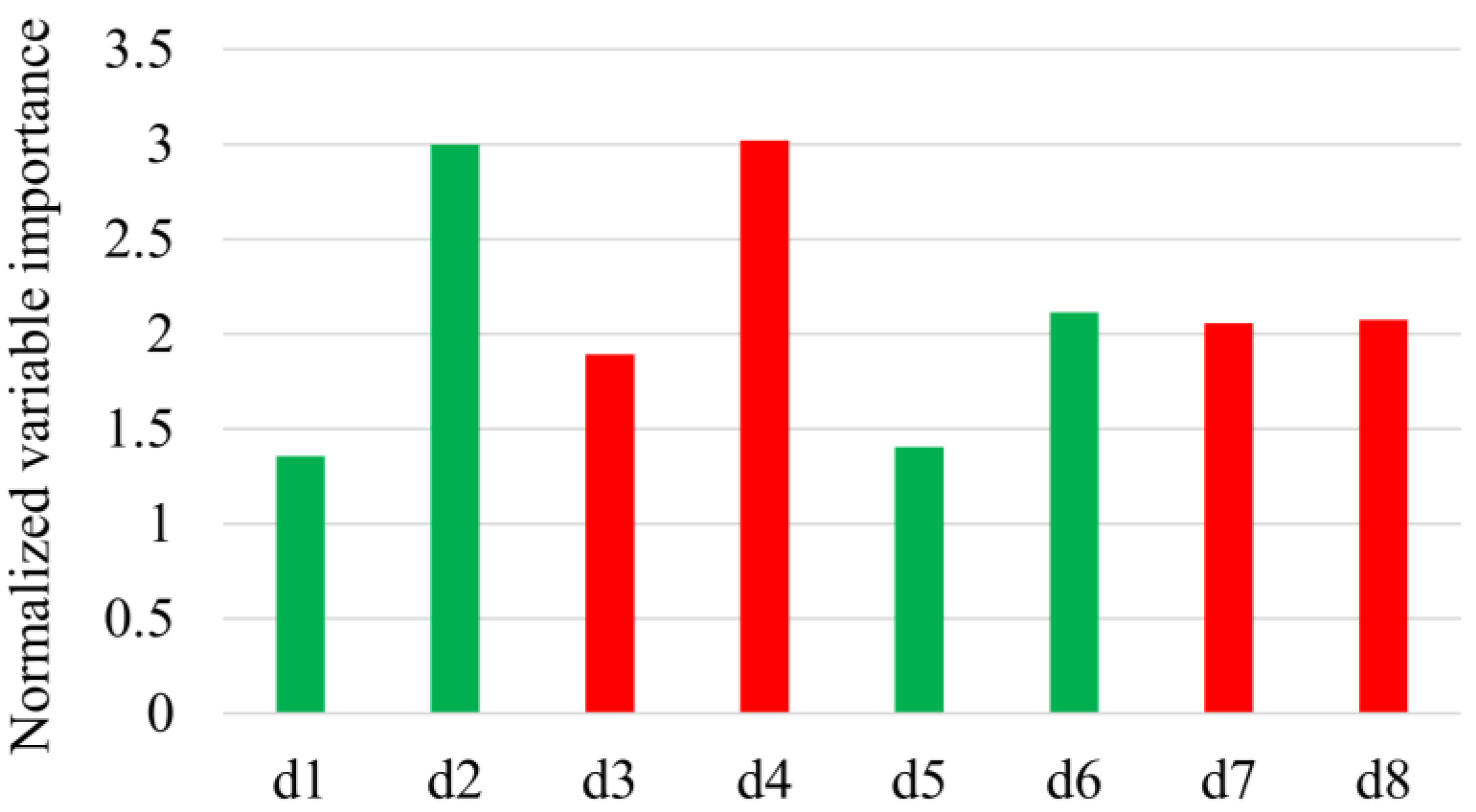
The comparison of the classifications using multi-temporal, multi-polarized data (FP SAR data) revealed the superiority of cross-polarized observations relative to those of co-polarized observations (see Table 5), which is supported by the RF variable importance analysis (see Figure 3). This is likely because cross-polarized observations are produced by volume scattering within the crop canopy and have a higher sensitivity to crop structures. Furthermore, as reported by a previous study [42], the HV intensity is highly correlated with leaf area index (LAI). The HV-polarized signal is also less sensitive to the row direction of planting crops. This reduces the variations in the cross-polarized SAR backscattering signatures of the same crops planted in varying row directions [
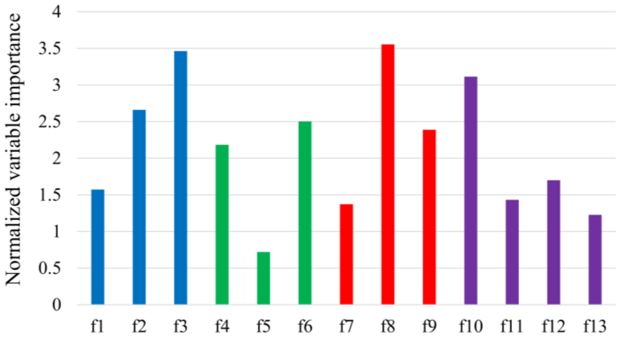
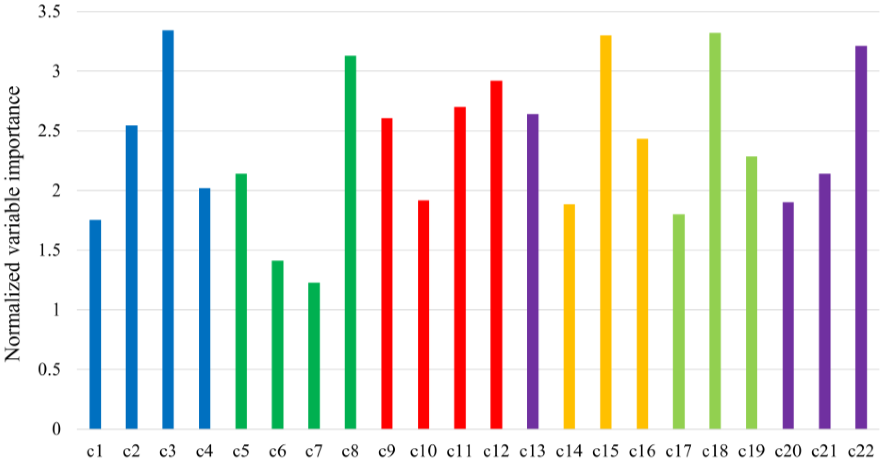
7]. Regarding the CP intensity features, σ R R 0 was the most important feature according to the RF variable importance (see Figure 7), and it also produced the highest classification accuracies when intensity features were compared (see Table 8 and Table 9).
Notably, in the mid-late growing season, differences in the cross-polarization SAR observations for various crop classes are potentially maximized due to both differences in canopy structures and moisture content, thus enhancing the discrimination between these classes [7]. Some studies, such as [43], reported that the late-July/early-August C-band data are optimal SAR observations for crop mapping, as crops exist in various stages of development, such as seeding (e.g., corn and soybeans), ripening (e.g., canola), and senesce or harvest (e.g., wheat and oats), at this time [7]. However, the phenological cycles of crops vary depending on local conditions (e.g., weather, soil water content) and management strategies (e.g., farmers’ decisions). For example, some crops may be planted much later due to a very long winter in years with extremely abnormal weather conditions [44]. The VV-polarization (i.e., see Table 5, S2, and Figure 3) was found to be the second-best polarization and was approximately 14.5% more accurate in terms of overall accuracy relative to HH (i.e., S1) for crop mapping. The results of our research endorse those of previous studies that confirmed the higher potential of HV- and VV-polarizations for crop mapping relative to HH-polarization [7,45]. Notably, some features of the CP SAR data, such as σ R V 0 , S 3 , and S 0 , are sensitive to the surface scattering [46] and were also found to be important CP SAR features (see Figure 7). This is particularly true for S 3 , as it was among the top-five most important CP SAR features. This finding is potentially explained by the fact that S3 is highly sensitive to the crop biomass, as [26] reported the best result for biomass inversion with S3 among all other CP SAR features.
Our results revealed the equal or slightly better ability of polarimetric decomposition methods compared to intensity channels for crop mapping either with FP or CP SAR data (e.g., see Table 9, S48 vs S51 and S52). In comparison, [18] reported the superiority of decomposition methods (e.g., Krogager decomposition) relative to intensity channels for crop mapping using ALOS PALSAR L-band data (~4% to 7% improvements). Nevertheless, they noted that C-band intensity observations (i.e., ASAR and RADARSAT-1) were advantageous relative to the L-band decomposition methods for crop classification, possibly due to the larger number of C-band acquisitions compared to those of L-band in that study. In general, the results of our study found that polarimetric decompositions are useful for discriminating differing crop types by characterizing various dominant scattering mechanisms during the stages of their developments.
The results also indicated that an improvement in overall accuracy was partial when polarimetric decomposition parameters were integrated with intensity observations. For example, S8 in Table 5 (all extracted features from the FP SAR data) was approximately 2.5% and 1.6% more accurate than S4 and S7, respectively. The minimal gain was also achieved by integrating intensity and decomposition features from the CP SAR data relative to those classifications based on either intensity (S37 vs S43 and S48 vs S54) or polarimetric decomposition features (S40 vs S43 and S52 vs S54). This finding corresponded to past studies that reported either a slight decline [18] or minimal improvement in overall accuracies [44] using L-band SAR data for crop mapping through the synergistic use of polarimetry and intensity features.
Regarding polarimetric decomposition methods, the variable importance analysis of RF indicated the highest and lowest contribution of volume and double-bounce scattering mechanisms, respectively, for crop mapping using both FP and CP SAR data. Previous research also found the lower contribution of double-bounce scattering for crop mapping [18], which was corroborated in our study. Double-bounce scattering, however, is of significance for monitoring wetland flooded vegetation and forest due to ground–trunk/stem interactions [47,48]. Surface/single scattering, which is produced by direct scattering from both soil and upper sections of crop canopies, was also found to be useful. Specifically, surface scattering is the dominant scattering mechanism during periods of crop emergence (early in the growing season), given that the ground is almost bare (very low vegetative cover) and, as such, there is negligible depolarization and random scattering. By mid-season, surface/odd-bounce scattering may be present; however, the enhanced interaction of the incident wave with the top layers of the crop canopies rather than surface scattering from soil is more pronounced [43]. During the mid-season, volume scattering becomes dominant due to reproduction, stem elongation, as well as significant seed and leaf development, increasing the chance of multiple interactions of the SAR signal within the randomly oriented crop canopies.
The results of H/A/alpha decomposition were well aligned with those of previous studies (e.g., [18,44]). Specifically, the RF variable importance indicated the greater contribution of alpha angle relative to those of entropy and anisotropy in this study (see Figure 3). McNairn and her colleagues in [18] also reported that alpha angle had discrimination potential for all crops during the entire growing season. They highlighted that the alpha angle could distinguish lower (e.g., forage crops) and more abundant (e.g., soybeans and corn) biomass crops at the beginning and end of the season. Canisius et al. in 2018 [49] also found that the alpha angle had a strong correlation with the LAI of wheat and, to a lesser extent, canola. Similar to our results, recent studies found the minimal discrimination potential of anisotropy for crop mapping using C- [49] and L-band [44] SAR data. Interestingly, α s was also ranked as the important features of the CP SAR data (see Figure 7, c12). The α s is similar to the alpha component of the Cloude-Pottier decomposition (i.e, an approximation to the α ) and determines the dominant scattering mechanims.
Comparison of classifications using simulated data at −19 and −24 dB revealed the marginal differences between the classification results of similar cases. This finding suggested that almost all crops had backscatter intensities higher than -19 dB (even at their early stages of development, for example, in May), which was at or higher than the noise floor of simulated SAR data in this study. Other studies, such as [42], also found HV backscatter intensity higher than or at −20 dB for similar crops (e.g., wheat and soybeans) during the early stages of the crop phenology using RADARSAT-2 data. The higher noise floor of simulated SAR data at −19 dB, however, is not problematic after the early stages of the crop development (e.g., mid-season). The reason is that all crops generally produce low backscattering intensities during emergence; however, intensities significantly increase as vegetative density increases during the growing season [42], resulting in backscattering values considerably higher than -19 dB in all polarization channels.
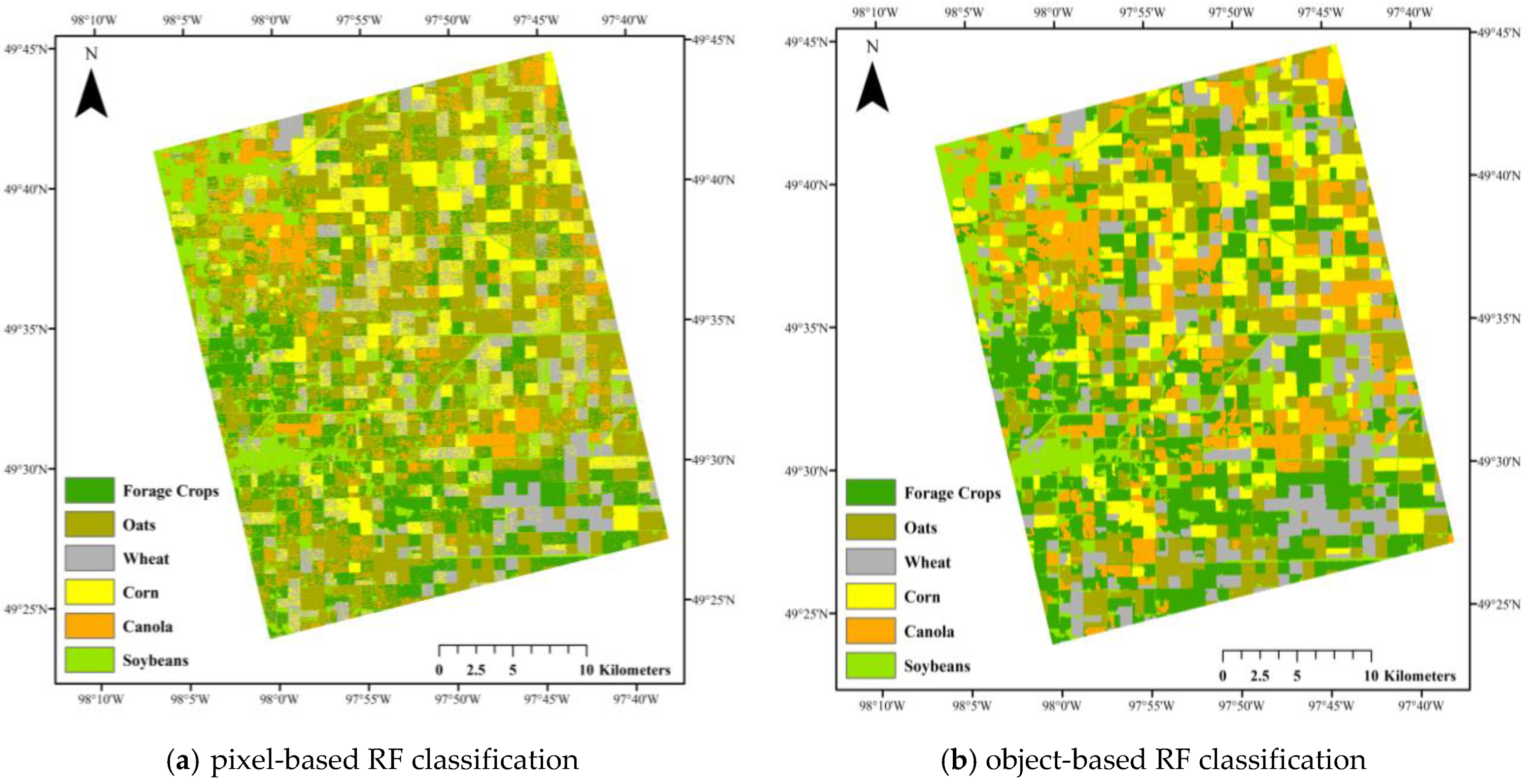
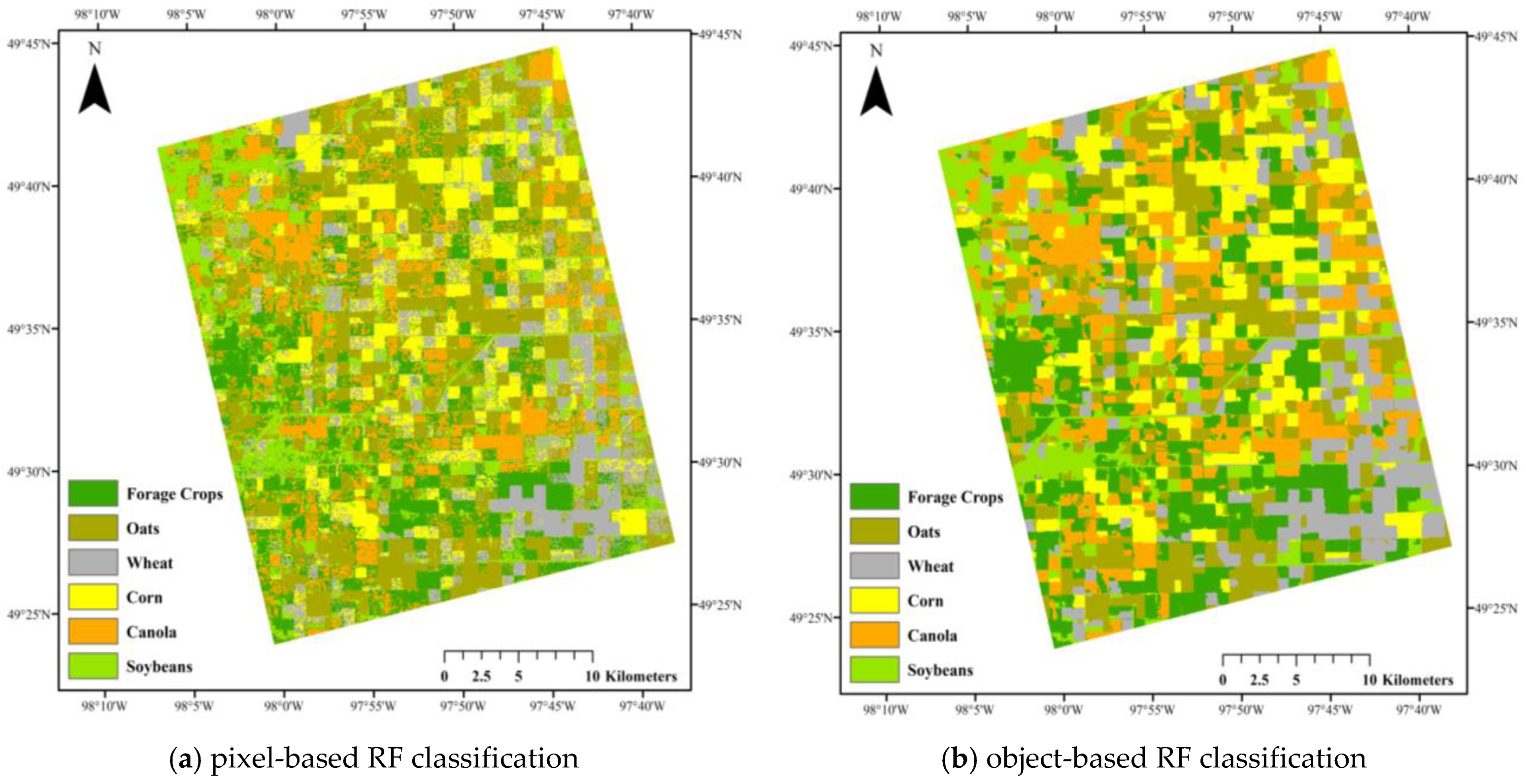
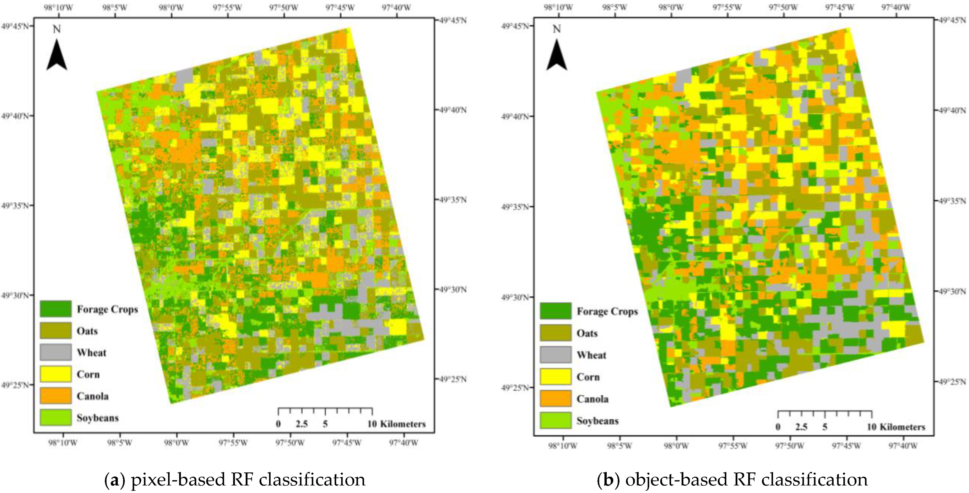
Importantly, the results in the final classification scheme using the object-based RF classification were promising, especially using both FP and CP SAR data (see Table 10). For example, 5 of 6 classes had producer’s accuracies approaching (i.e., wheat) or exceeding (i.e., oats, corn, canola, and soybeans) 85% using FP SAR data. Overall, target accuracies of 85% were achieved using this classification scenario [7]. CP SAR data were also useful with high producer’s accuracies for most classes (e.g., corn, canola, wheat, and oats). The success of CP SAR data for crop mapping is potentially explained by the fact that a circular polarization wave enhances interaction with the canopy and, as such, increases the chance of multiple scattering within crop canopies [50]. This is particularly true for crops such as canola and corn, that have stem, leaf, and seed with random orientations.
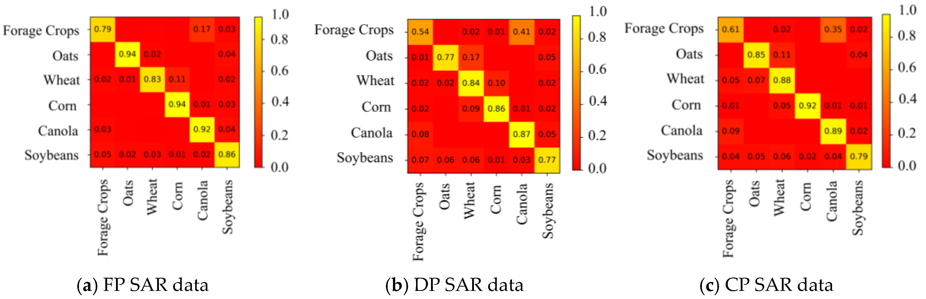
One possible reason for the lowest accuracy of the forage crops in all three cases (see Figure 12) is the difficulty in assigning an explicit SAR backscattering signature to this class, as it includes several species. Conversely, the confusion matrices demonstrated that larger biomass crops, such as corn and canola, were identified with producer accuracies above 85% using three SAR data types (see Figure 12). This is because these larger biomass crops have a random structure after flowering, which produces a large amount of volume scattering, thus simplifying their discrimination using PolSAR imagery. Wheat and oats were also classified with accuracies exceeding 83% using both FP and CP SAR data; however, confusion was present between these two classes in some cases. This is because these two classes have very similar canopy structures and relatively the same growing stages, which result in similar SAR backscattering responses.
Both wheat and oats are lower biomass crops with less random crop structures, allowing a deeper penetration of the SAR signal into their canopy. This enhances backscattering responses from the underlying soil, thus contributing to the misclassification between the two classes [43]. Accordingly, these classes have been merged into a single class (cereals) in several crop classification studies (e.g., [7]). One interesting observation was the higher producer accuracy of wheat using CP SAR data compared to that of FP SAR data. Although there was no apparent reason for this observation, this agreed, to some extent, with [20] who found the highest correlation between wheat dry biomass and the circular compared to the linear polarization ratios for the same test site in SMAPVEX12.
An improvement in overall accuracy could be achieved upon the inclusion of August SAR observations into the classification scheme. As mentioned above, the highest contrast in the crop structures is expected at this time of the crop phenological cycle under normal weather conditions, given that some crops (e.g., corn and soybeans) are likely to be in their seed developmental stages, whereas others (e.g., wheat and oats) are in their senescence and harvest stages [7]. Further improvement in the overall accuracy of crop mapping is expected upon the inclusion of multi-frequency SAR data. This is because, while C-band SAR data are useful for both lower and larger biomass crops, L-band may improve the discrimination capability for larger biomass crops (e.g., soybeans and corn), given the higher penetration depth of the latter SAR signal [18]. However, such multi-frequency SAR data demand acquisition from different satellites because currently operating SAR sensors do not collect multi-frequency data. Previous studies also reported that the synergistic use of optical and SAR data is promising, given that the former observation is sensitive to spectral and biophysical characterization of crops [51,52] while the latter is sensitive to their structural characteristics. This also addresses the intrinsic limitation of optical imagery (i.e., cloud and haze), which results in data gaps in classifications based only on optical data [7]. Notably, multi-source satellite imagery (optical and SAR) could be of particular use when there is a lack of multi-temporal data. An operational example of this approach is the annual crop inventory produced by Agriculture and Agri-Food Canada, which incorporates C-band RADARSAT-2 DP SAR data (VV/VH) with available optical data (depending on the cloud cover; [19]). Although the results of this study suggested that the simulated CP SAR data will be of great significance for crop mapping, these results should be further justified in different case studies when real CP SAR data are available by the RADARSAT Constellation Mission.

6. Conclusions

In this study, the capability of early- to mid-season (i.e., May to July) RADARSAT-2 SAR images were examined for crop mapping in an agricultural region in Manitoba, Canada. Various classification scenarios were defined based on extracted features from full polarimetry SAR data, as well as simulated dual and compact polarimetry SAR data. Both overall and individual class accuracies were compared for multi-temporal, multi-polarization SAR data using the pixel-based and object-based random forest classification schemes.
The classification results revealed the importance of multi-temporal SAR observations for accurate crop mapping. Mid-season C-band SAR observations (late July in this study) were found to be advantageous for crop mapping, as crops have already accumulated significant biomass and have transitioned into varying developmental stages, such as reproduction, seed development, and senescence. The results demonstrated a similar capability of decomposition parameters for crop mapping relative to the intensity channels for both FP and CP SAR data. The synergistic use of polarimetric decomposition and intensity features resulted in a marginal improvement in overall accuracies relative to classifications based only on SAR intensity and decomposition features. The variable importance analysis of RF found that for both FP and CP SAR data the volumetric component of the decomposition features and σ R R 0 and σ H V 0 intensities contribute more to the crop mapping. The reason is that these features have the highest sensitivity to variances in crop structures due to crop types and changing phenology.
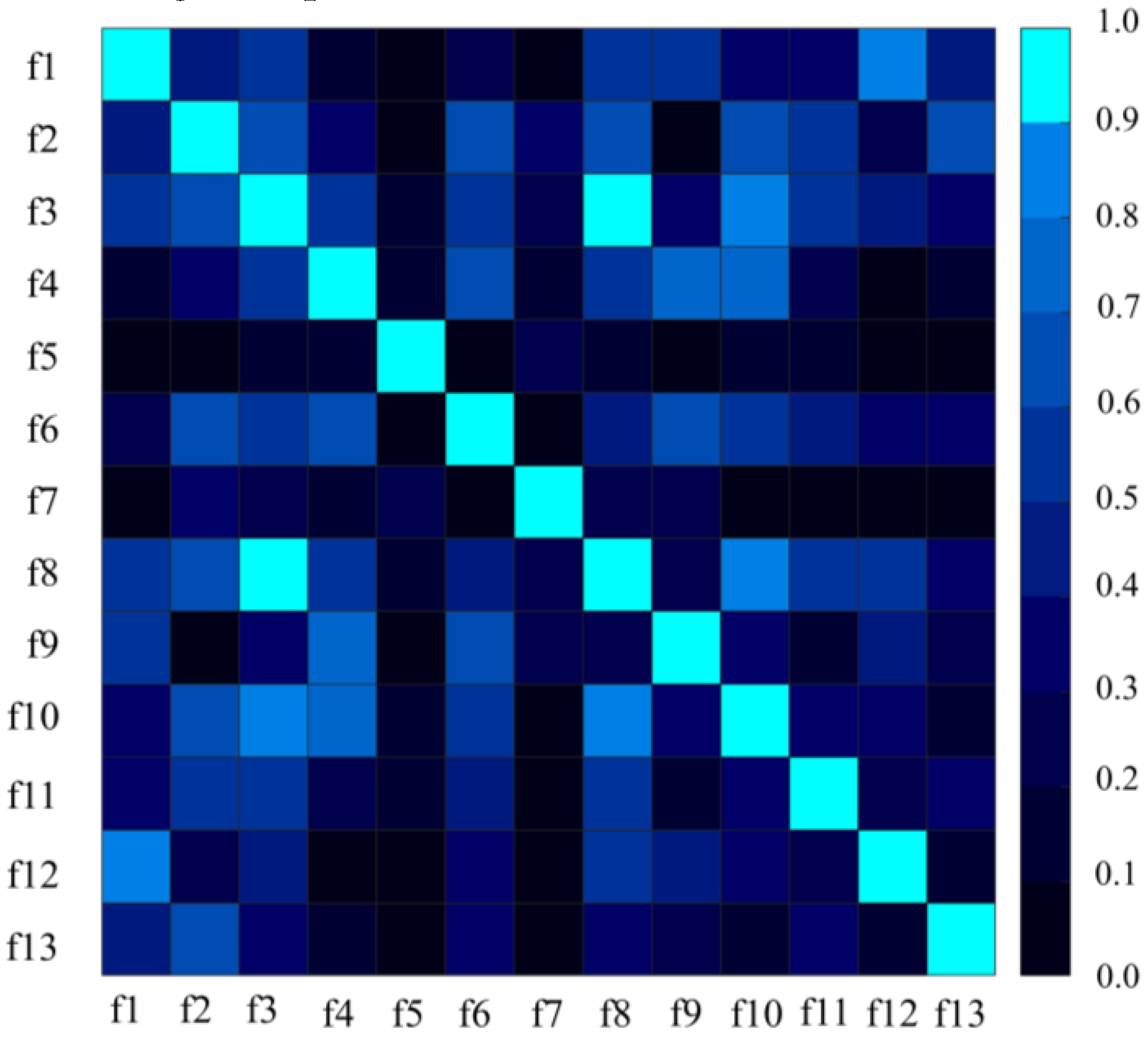
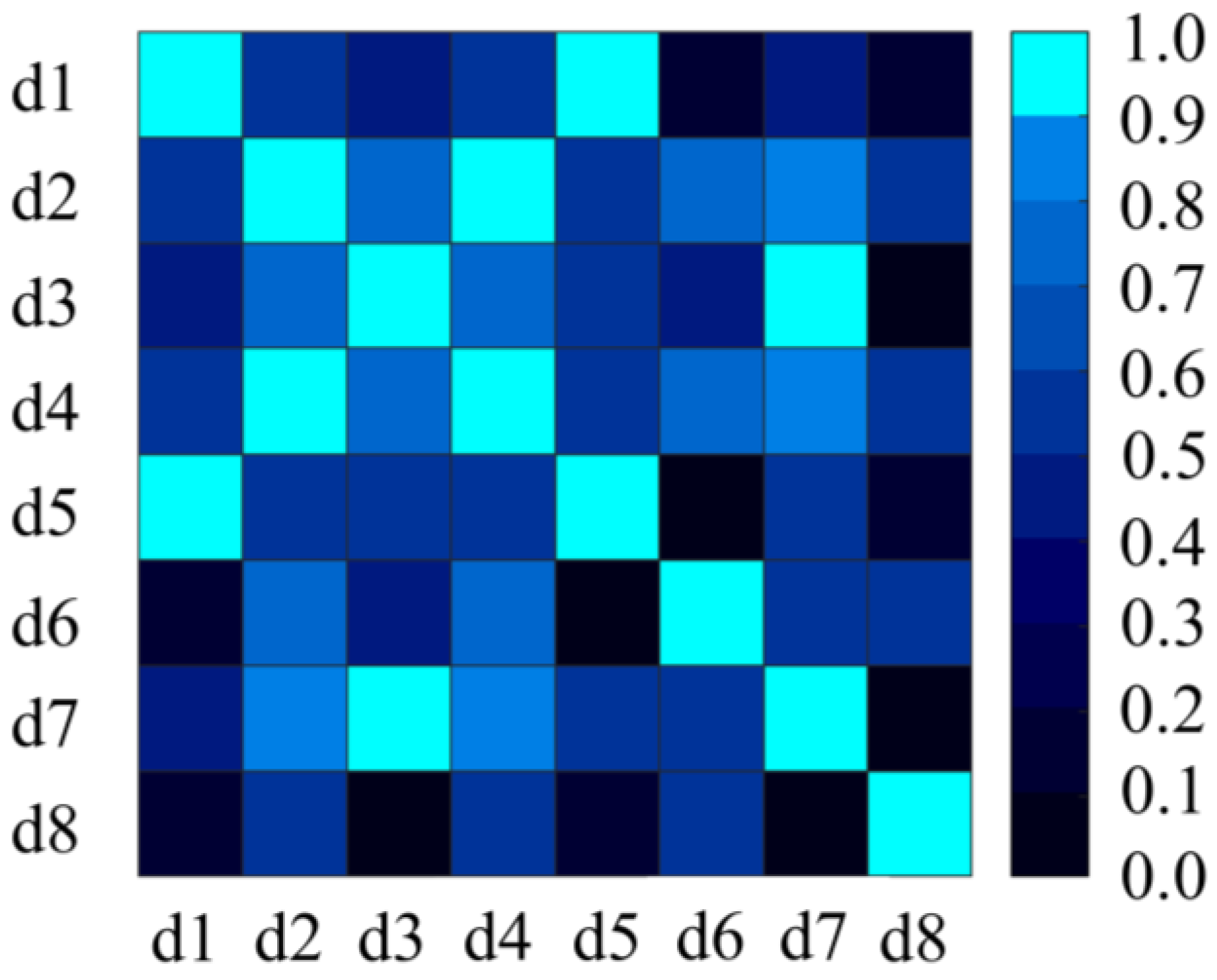
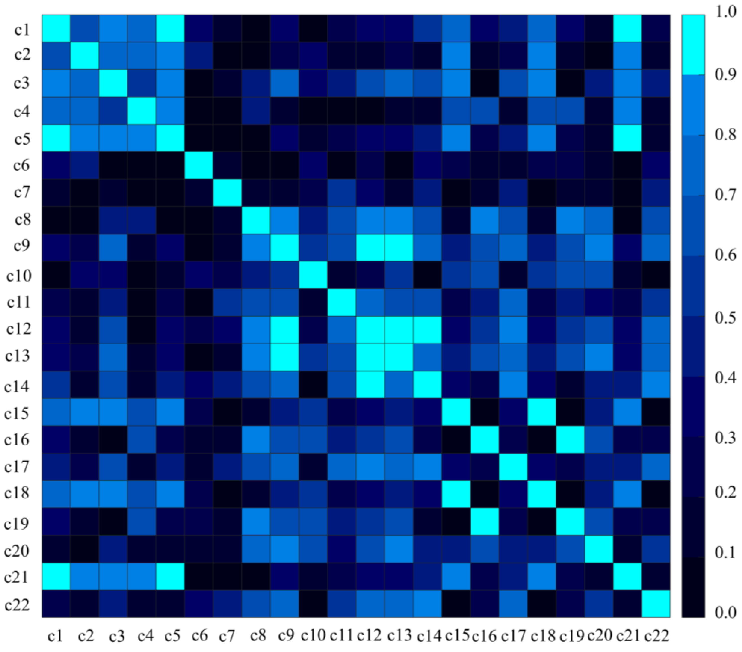
A Spearman correlation coefficient analysis revealed that there were high correlations between extracted features from FP, DP, and CP SAR data. This explained the lower gain in overall classification accuracy when highly correlated features were incorporated into the classification scheme. The highest classification accuracies of 88.2%, 82.1%, and 77.3% were achieved using uncorrelated features extracted from the FP, CP, and DP SAR data, respectively, with the object-based RF classification approach. Although the classification accuracy obtained from FP SAR data was higher than that of CP SAR data, the latter is more suitable for operational monitoring. Wider swath widths associated with CP will allow for sub-weekly observations, thus providing high temporal resolution data, an important factor for accurate crop mapping at a national scale.
The results of this research suggest that the CP mode available on the RADARSAT Constellation Mission will provide data of great interest for operational crop mapping. The analysis presented in this study contributes to further scientific research for agricultural applications and, importantly, demonstrates that RCM’s CP configuration will be a critical source of data to support Canada’s commitment to operational crop monitoring.

Author Contributions

M.M., F.M., and S.H. conceived and designed the experiments. M.M. and F.M. performed the experiments, analyzed the data, and wrote the paper. H.M., A.D., M.R., and B.S. contributed editorial input and scientific insights to further improve the paper. All authors reviewed and commented on the manuscript.

Funding

This project was undertaken with the financial support of the Research & Development Corporation of Government of Newfoundland and Labrador (now InnovateNL) under Grant to M. Mahdianpari (RDC 5404-2108-101).

Acknowledgments

The authors would like to thank the entire SMAPVEX12 crew who worked tirelessly to make the campaign a great success. The Canadian participation in SMAPVEX12 was partially funded by the Government Relative Initiatives Program (GRIP) of the Canadian Space Agency and the Growing Forward 2 (GF2) of the Agriculture and Agri-Food Canada.

Conflicts of Interest

The authors declare no conflicts of interest.

References

  1. Haboudane, D.; Tremblay, N.; Miller, J.R.; Vigneault, P. Remote estimation of crop chlorophyll content using spectral indices derived from hyperspectral data. IEEE Trans. Geosci. Remote Sens. 2008, 46, 423–437. [Google Scholar] [CrossRef]
  2. Belgiu, M.; Csillik, O. Sentinel-2 cropland mapping using pixel-based and object-based time-weighted dynamic time warping analysis. Remote Sens. Environ. 2018, 204, 509–523. [Google Scholar] [CrossRef]
  3. Steele-Dunne, S.C.; McNairn, H.; Monsivais-Huertero, A.; Judge, J.; Liu, P.-W.; Papathanassiou, K. Radar remote sensing of agricultural canopies: A review. IEEE J. Sel. Top. Appl. Earth Obs. Remote Sens. 2017, 10, 2249–2273. [Google Scholar] [CrossRef]
  4. Raney, R.K.; Cahill, J.T.S.; Patterson, G.; Bussey, D.B.J. The m-chi decomposition of hybrid dual-polarimetric radar data with application to lunar craters. J. Geophys. Res. Planets 2012, 117, E12. [Google Scholar] [CrossRef]
  5. Mahdianpari, M.; Salehi, B.; Mohammadimanesh, F. The Effect of PolSAR Image De-speckling on Wetland Classification: Introducing a New Adaptive Method. Can. J. Remote Sens. 2017, 43, 485–503. [Google Scholar] [CrossRef]
  6. Salberg, A.-B.; Rudjord, Ø.; Solberg, A.H.S. Oil spill detection in hybrid-polarimetric SAR images. IEEE Trans. Geosci. Remote Sens. 2014, 52, 6521–6533. [Google Scholar] [CrossRef]
  7. McNairn, H.; Champagne, C.; Shang, J.; Holmstrom, D.; Reichert, G. Integration of optical and Synthetic Aperture Radar (SAR) imagery for delivering operational annual crop inventories. ISPRS J. Photogramm. Remote Sens. 2009, 64, 434–449. [Google Scholar] [CrossRef]
  8. Mahdianpari, M.; Salehi, B.; Mohammadimanesh, F.; Brisco, B.; Mahdavi, S.; Amani, M.; Granger, J.E. Fisher Linear Discriminant Analysis of coherency matrix for wetland classification using PolSAR imagery. Remote Sens. Environ. 2018, 206, 300–317. [Google Scholar] [CrossRef]
  9. Dubois-Fernandez, P.C.; Souyris, J.-C.; Angelliaume, S.; Garestier, F. The compact polarimetry alternative for spaceborne SAR at low frequency. IEEE Trans. Geosci. Remote Sens. 2008, 46, 3208–3222. [Google Scholar] [CrossRef]
  10. Nord, M.E.; Ainsworth, T.L.; Lee, J.-S.; Stacy, N.J.S. Comparison of compact polarimetric synthetic aperture radar modes. IEEE Trans. Geosci. Remote Sens. 2009, 47, 174–188. [Google Scholar] [CrossRef]
  11. Mohammadimanesh, F.; Salehi, B.; Mahdianpari, M.; Brisco, B.; Gill, E. Full and Simulated Compact Polarimetry SAR Responses to Canadian Wetlands: Separability Analysis and Classification. Remote Sens. 2019, 11, 516. [Google Scholar] [CrossRef]
  12. Charbonneau, F.J.; Brisco, B.; Raney, R.K.; McNairn, H.; Liu, C.; Vachon, P.W.; Shang, J.; DeAbreu, R.; Champagne, C.; Merzouki, A. Compact polarimetry overview and applications assessment. Can. J. Remote Sens. 2010, 36, S298–S315. [Google Scholar] [CrossRef]
  13. Raney, R. Hybrid-polarity SAR architecture. In Proceedings of the Geoscience and Remote Sensing Symposium, Denver, CO, USA, 31 July–4 August 2006; pp. 3846–3848. [Google Scholar]
  14. Nunziata, F.; Migliaccio, M.; Li, X. Sea oil slick observation using hybrid-polarity SAR architecture. IEEE J. Ocean. Eng. 2015, 40, 426–440. [Google Scholar] [CrossRef]
  15. Mohammadimanesh, F.; Salehi, B.; Mahdianpari, M.; Brisco, B.; Motagh, M. Wetland water level monitoring using interferometric synthetic aperture radar (InSAR): A review. Can. J. Remote Sens. 2018, 1–16. [Google Scholar] [CrossRef]
  16. Thompson, A.A. Overview of the RADARSAT constellation mission. Can. J. Remote Sens. 2015, 41, 401–407. [Google Scholar] [CrossRef]
  17. Foody, G.M.; McCulloch, M.B.; Yates, W.B. Crop classification from C-band polarimetric radar data. Int. J. Remote Sens. 1994, 15, 2871–2885. [Google Scholar] [CrossRef]
  18. McNairn, H.; Shang, J.; Jiao, X.; Champagne, C. The contribution of ALOS PALSAR multipolarization and polarimetric data to crop classification. IEEE Trans. Geosci. Remote Sens. 2009, 47, 3981–3992. [Google Scholar] [CrossRef]
  19. Davidson, A.M.; Fisette, T.; McNairn, H.; Daneshfar, B. Detailed crop mapping using remote sensing data (Crop Data Layers). In Handbook on Remote Sensing for Agricultural Statistics; Handbook of the Global Strategy to Improve Agricultural and Rural Statistics (GSARS): Rome, Italy, 2017; Chapter 4; pp. 91–117. [Google Scholar]
  20. Wiseman, G.; McNairn, H.; Homayouni, S.; Shang, J. RADARSAT-2 polarimetric SAR response to crop biomass for agricultural production monitoring. IEEE J. Sel. Top. Appl. Earth Obs. Remote Sens 2014, 7, 4461–4471. [Google Scholar] [CrossRef]
  21. McNairn, H.; Jackson, T.J.; Wiseman, G.; Belair, S.; Berg, A.; Bullock, P.; Colliander, A.; Cosh, M.H.; Kim, S.-B.; Magagi, R. The Soil Moisture Active Passive Validation Experiment 2012 (SMAPVEX12): Prelaunch calibration and validation of the SMAP soil moisture algorithms. IEEE Trans. Geosci. Remote Sens. 2015, 53, 2784–2801. [Google Scholar] [CrossRef]
  22. Mahdianpari, M.; Salehi, B.; Mohammadimanesh, F.; Motagh, M. Random forest wetland classification using ALOS-2 L-band, RADARSAT-2 C-band, and TerraSAR-X imagery. ISPRS J. Photogramm. Remote Sens. 2017, 130, 13–31. [Google Scholar] [CrossRef]
  23. Mohammadimanesh, F.; Salehi, B.; Mahdianpari, M.; Homayouni, S. Unsupervised wishart classfication of wetlands in Newfoundland, Canada using polsar data based on fisher linear discriminant analysis. Int. Archiv. Photogramm. Remote Sens.Spat. Inf. Sci. 2016, 41, 305–310. [Google Scholar] [CrossRef]
  24. Raney, R.K. Hybrid-polarity SAR architecture. IEEE Trans. Geosci. Remote Sens. 2007, 45, 3397–3404. [Google Scholar] [CrossRef]
  25. Lee, J.-S.; Pottier, E. Polarimetric Radar Imaging: From Basics to Applications; CRC Press: Boca Raton, FL, USA, 2009; ISBN 1420054988. [Google Scholar]
  26. Zhang, W.; Li, Z.; Chen, E.; Zhang, Y.; Yang, H.; Zhao, L.; Ji, Y. Compact Polarimetric Response of Rape (Brassica napus L.) at C-Band: Analysis and Growth Parameters Inversion. Remote Sens. 2017, 9, 591. [Google Scholar] [CrossRef]
  27. Ballester-Berman, J.D.; Lopez-Sanchez, J.M. Time series of hybrid-polarity parameters over agricultural crops. IEEE Geosci. Remote Sens. Lett. 2012, 9, 139–143. [Google Scholar] [CrossRef]
  28. Cloude, S.R.; Goodenough, D.G.; Chen, H. Compact decomposition theory. IEEE Geosci. Remote Sens. Lett. 2012, 9, 28–32. [Google Scholar] [CrossRef]
  29. Espeseth, M.M.; Brekke, C.; Johansson, A.M. Assessment of RISAT-1 and Radarsat-2 for sea ice observations from a hybrid-polarity perspective. Remote Sens. 2017, 9, 1088. [Google Scholar] [CrossRef]
  30. Truong-Loi, M.-L.; Freeman, A.; Dubois-Fernandez, P.C.; Pottier, E. Estimation of soil moisture and Faraday rotation from bare surfaces using compact polarimetry. IEEE Trans. Geosci. Remote Sens. 2009, 47, 3608–3615. [Google Scholar] [CrossRef]
  31. Dabboor, M.; Geldsetzer, T. Towards sea ice classification using simulated RADARSAT Constellation Mission compact polarimetric SAR imagery. Remote Sens. Environ. 2014, 140, 189–195. [Google Scholar] [CrossRef]
  32. Marechal, C.; Pottier, E.; Hubert-Moy, L.; Rapinel, S. One year wetland survey investigations from quad-pol RADARSAT-2 time-series SAR images. Can. J. Remote Sens. 2012, 38, 240–252. [Google Scholar] [CrossRef]
  33. Blaschke, T. Object based image analysis for remote sensing. ISPRS J. Photogramm. Remote Sens. 2010, 65, 2–16. [Google Scholar] [CrossRef] [Green Version]
  34. Mahdianpari, M.; Salehi, B.; Mohammadimanesh, F.; Homayouni, S.; Gill, E. The First Wetland Inventory Map of Newfoundland at a Spatial Resolution of 10 m Using Sentinel-1 and Sentinel-2 Data on the Google Earth Engine Cloud Computing Platform. Remote Sens. 2019, 11, 43. [Google Scholar] [CrossRef]
  35. Benz, U.C.; Hofmann, P.; Willhauck, G.; Lingenfelder, I.; Heynen, M. Multi-resolution, object-oriented fuzzy analysis of remote sensing data for GIS-ready information. ISPRS J. Photogramm. Remote Sens. 2004, 58, 239–258. [Google Scholar] [CrossRef]
  36. Breiman, L. Random forests. Mach. Learn. 2001, 45, 5–32. [Google Scholar] [CrossRef]
  37. Belgiu, M.; Drăguţ, L. Random forest in remote sensing: A review of applications and future directions. ISPRS J. Photogramm. Remote Sens. 2016, 114, 24–31. [Google Scholar] [CrossRef]
  38. Rodriguez-Galiano, V.F.; Ghimire, B.; Rogan, J.; Chica-Olmo, M.; Rigol-Sanchez, J.P. An assessment of the effectiveness of a random forest classifier for land-cover classification. ISPRS J. Photogramm. Remote Sens. 2012, 67, 93–104. [Google Scholar] [CrossRef]
  39. Chan, J.C.-W.; Paelinckx, D. Evaluation of Random Forest and Adaboost tree-based ensemble classification and spectral band selection for ecotope mapping using airborne hyperspectral imagery. Remote Sens. Environ. 2008, 112, 2999–3011. [Google Scholar] [CrossRef]
  40. Congalton, R.G. A review of assessing the accuracy of classifications of remotely sensed data. Remote Sens. Environ. 1991, 37, 35–46. [Google Scholar] [CrossRef]
  41. Mohammadimanesh, F.; Salehi, B.; Mahdianpari, M.; Motagh, M.; Brisco, B. An efficient feature optimization for wetland mapping by synergistic use of SAR intensity, interferometry, and polarimetry data. Int. J. Appl. Earth Obs. Geoinf. 2018, 73, 450–462. [Google Scholar] [CrossRef]
  42. Liu, C.; Shang, J.; Vachon, P.W.; McNairn, H. Multiyear crop monitoring using polarimetric RADARSAT-2 data. IEEE Trans. Geosci. Remote Sens. 2013, 51, 2227–2240. [Google Scholar] [CrossRef]
  43. Jiao, X.; Kovacs, J.M.; Shang, J.; McNairn, H.; Walters, D.; Ma, B.; Geng, X. Object-oriented crop mapping and monitoring using multi-temporal polarimetric RADARSAT-2 data. ISPRS J. Photogramm. Remote Sens. 2014, 96, 38–46. [Google Scholar] [CrossRef]
  44. Whelen, T.; Siqueira, P. Use of time-series L-band UAVSAR data for the classification of agricultural fields in the San Joaquin Valley. Remote Sens. Environ. 2017, 193, 216–224. [Google Scholar] [CrossRef]
  45. Foody, G.M. Supervised image classification by MLP and RBF neural networks with and without an exhaustively defined set of classes. Int. J. Remote Sens. 2004, 25, 3091–3104. [Google Scholar] [CrossRef]
  46. Geldsetzer, T.; Arkett, M.; Zagon, T.; Charbonneau, F.; Yackel, J.J.; Scharien, R.K. All-season compact-polarimetry C-band SAR observations of sea ice. Can. J. Remote Sens. 2015, 41, 485–504. [Google Scholar] [CrossRef]
  47. Mahdianpari, M.; Salehi, B.; Mohammadimanesh, F.; Brisco, B. An Assessment of Simulated Compact Polarimetric SAR Data for Wetland Classification Using Random Forest Algorithm. Can. J. Remote Sens. 2017, 43, 468–484. [Google Scholar] [CrossRef]
  48. Mohammadimanesh, F.; Salehi, B.; Mahdianpari, M.; Brisco, B.; Motagh, M. Multi-temporal, multi-frequency, and multi-polarization coherence and SAR backscatter analysis of wetlands. ISPRS J. Photogramm. Remote Sens. 2018, 142, 78–93. [Google Scholar] [CrossRef]
  49. Canisius, F.; Shang, J.; Liu, J.; Huang, X.; Ma, B.; Jiao, X.; Geng, X.; Kovacs, J.M.; Walters, D. Tracking crop phenological development using multi-temporal polarimetric Radarsat-2 data. Remote Sens. Environ. 2018, 210, 508–518. [Google Scholar] [CrossRef]
  50. Homayouni, S.; McNairn, H.; Hosseini, M.; Jiao, X.; Powers, J. Quad and compact multitemporal C-band PolSAR observations for crop characterization and monitoring. Int. J. Appl. Earth Obs. Geoinf. 2019, 74, 78–87. [Google Scholar] [CrossRef]
  51. Mahdianpari, M.; Salehi, B.; Rezaee, M.; Mohammadimanesh, F.; Zhang, Y. Very Deep Convolutional Neural Networks for Complex Land Cover Mapping Using Multispectral Remote Sensing Imagery. Remote Sens. 2018, 10, 1119. [Google Scholar] [CrossRef]
  52. Rezaee, M.; Mahdianpari, M.; Zhang, Y.; Salehi, B. Deep Convolutional Neural Network for Complex Wetland Classification Using Optical Remote Sensing Imagery. IEEE J. Sel. Top. Appl. Earth Obs. Remote Sens. 2018, 11, 3030–3039. [Google Scholar] [CrossRef]
Figure 1. The geographic location of the study area.
Remotesensing 11 01582 g001
Figure 2. Mean JM distances for each crop to the others using intensity features extracted from (a) DP, (b) CP, and (c) FP SAR data.
Remotesensing 11 01582 g002aRemotesensing 11 01582 g002b
Figure 3. Normalized RF variable importance for extracted features from the FP SAR data (July 21). Please note that f1: σ H H 0 , f2: σ V V 0 , f3: σ H V 0 , f4: H , f5: A , f6: α , f7: F r e e m a n D u r d e n D o u b l e , f8: F r e e m a n D u r d e n V o l u m e , f9: F r e e m a n D u r d e n S u r f a c e , f10: Y a m a g u c h i V o l u m e , f11: Y a m a g u c h i H e l i x , f12: Y a m a g u c h i S u r f a c e , and f13: Y a m a g u c h i D o u b l e .
Remotesensing 11 01582 g003
Figure 4. The absolute value of the Spearman correlation between the extracted features from the FP SAR data. Please note that 0 and 1 indicate zero and the highest correlation, respectively.
Remotesensing 11 01582 g004
Figure 5. Normalized RF variable importance for extracted features from the simulated DP SAR data (July 21). Please note that d1: σ H H 0 , d2: σ H V 0 , d3: σ V V 0 , d4: σ V H 0 , d5: S p a n 1 , d6: R a t i o 1 , d7: S p a n 2 , and d8: R a t i o 2 . See Table 2 for abbreviations of features.
Remotesensing 11 01582 g005
Figure 6. The absolute value of the Spearman correlation between the extracted features from the simulated DP SAR data.
Remotesensing 11 01582 g006
Figure 7. Normalized RF variable importance for extracted features from the simulated CP SAR data (July 21). Please note that c1: σ R H 0 , c2: σ R V 0 , c3: σ R R 0 , c4: σ R L 0 , c5: S 0 , c6: S 1 , c7: S 2 , c8: S 3 , c9: μ c , c10: m , c11: δ , c12: α s , c13: μ , c14: m χ E , c15: m χ V , c16: m χ O , c17: m δ E , c18: m δ V , c19: m δ O , c20: ρ , c21: SEI, and c22: SEP. See Table 2 for abbreviations of features.
Remotesensing 11 01582 g007
Figure 8. The absolute value of the Spearman correlation between the extracted features from the simulated CP SAR data.
Remotesensing 11 01582 g008
Figure 9. The final land cover maps obtained from the uncorrelated FP SAR features using (a) pixel-based and (b) object-based RF classifications.
Remotesensing 11 01582 g009
Figure 10. The final land cover maps obtained from the uncorrelated DP SAR features using (a) pixel-based and (b) object-based RF classifications.
Remotesensing 11 01582 g010
Figure 11. The final land cover maps obtained from the uncorrelated CP SAR features using (a) pixel-based and (b) object-based RF classifications.
Remotesensing 11 01582 g011
Figure 12. The confusion matrices for the final classification maps with the object-based RF classification using the uncorrelated features extracted from (a) FP, (b) DP, and (c) CP SAR data.
Remotesensing 11 01582 g012
Table 1. Testing and training pixel counts for each crop in this study.
Class#Training Pixels#Testing PixelsTotal
Forage Crops12,29410,46122,755
Oats13,23812,96226,200
Wheat15,63211,97927,611
Corn12,847848921,336
Canola15,05613,68128,737
Soybeans14,06312,76626,829
Total83,13070,338153,468
Table 2. A description of simulated SAR features employed in this study.
Simulated DataFeature NameDescriptionFormulaReference
Dual-pol HH/HVIntensitySAR backscattering coefficients σ H H 0 , σ H V 0 N/A
Total power ( S p a n 1 ) | σ H H 0 | 2 +   | σ H V 0 | 2 N/A
Ratio ( R a t i o 1 ) | σ H H 0 | 2 | σ H V 0 | 2 N/A
Dual-pol VV/VHIntensitySAR backscattering coefficients σ V V 0 , σ V H 0 N/A
Total power ( S p a n 2 ) | σ V V 0 | 2 +   | σ V H 0 | 2 N/A
Ratio ( R a t i o 2 ) | σ V V 0 | 2 | σ V H 0 | 2 N/A
Compact-pol dataIntensitySAR backscattering coefficients σ R R 0 , σ R L 0 , σ R H 0 , σ R V 0 N/A
Stokes vector parametersThe first element S 0 = < | E R H | 2 + | E R V | 2 > [4]
The second element S 1 = < | E R H | 2 | E R V | 2 >
The third element S 2 = 2 R e < E R H E R V * >
The fourth element S 3 = 2 I m < E R H E R V * >
Stokes child parametersCircular polarization ratio μ c = S 0 S 3 S 0 + S 3 [12]
Degree of polarization m = S 1 2 + S 2 2 + S 3 2 S 0 2 [4]
Relative phase δ = tan 1 ( S 3 S 2 ) [12]
Ellipticity of the compact scattered wave α s = 1 2 tan 1 ( s 1 2 + s 2 2 S 3 ) [28]
CP decompositions m d e l t a m δ O = S 0 m ( 1 + sin δ ) 2 [12]
m δ E = S 0 m ( 1 sin δ ) 2
m δ V = S 0 ( 1 m )
m c h i m χ O = S 0 m ( 1 sin 2 χ ) 2 [4]
m χ E =   S 0 m ( 1 + sin 2 χ ) 2
m χ V = S 0 ( 1 m )
Wave descriptorsConformity coefficient μ = 2   I m < S R H S R V * > < S R H S R H * > + < S R V S R V * > [30]
Correlation coefficient ρ = | < S R H S R V * > < S R H S R H * > + < S R V S R V * > | [31]
Shannon entropy intensity S E I = 2 log ( π e T r ( T 2 ) 2 ) [31]
Shannon entropy polarimetry S E P = log ( 4 | T 2 | T r ( T 2 ) 2 )
Table 3. Different pixel-based classification scenarios examined in this study.
DataScenarioFeaturesNF: −19NF: −24# Features
FPS1HHN/AN/A4
S2VVN/AN/A4
S3HVN/AN/A4
S4IntensityN/AN/A12
S5Cloude-Pottier decompositionN/AN/A12
S6Freeman-Durden decompositionN/AN/A12
S7Yamaguchi decompositionN/AN/A16
S8All FP featuresN/AN/A52
DPS9HH 4
S10HV 4
S11VV 4
S12VH 4
S13HH, HV 8
S14VV, VH 8
S15Total power (HH, HV) 4
S16Total power (VV, VH) 4
S17Ratio (HH, HV) 4
S18Ratio (VV, VH) 4
S19All DP features (HH, HV) 16
S20All DP features (VV, VH) 16
DPS21HH 4
S22HV 4
S23VV 4
S24VH 4
S25HH, HV 8
S26VV, VH 8
S27Total power (HH, HV) 4
S28Total power (VV, VH) 4
S29Ratio (HH, HV) 4
S30Ratio (VV, VH) 4
S31All DP features (HH, HV) 16
S32All DP features (VV, VH) 16
CPS33RH 4
S34RV 4
S35RR 4
S36RL 4
S37All intensity 16
S38Stokes vector 16
S39Stokes child parameters 16
S40m-delta decomposition 12
S41m-chi decomposition 12
S42Wave descriptors 16
S43All CP features 88
CPS44RH 4
S45RV 4
S46RR 4
S47RL 4
S48All intensity 16
S49Stokes vector 16
S50Stokes child parameters 16
S51m-delta decomposition 12
S52m-chi decomposition 12
S53Wave descriptors 16
S54All CP features 88
Table 4. Classification results obtained from intensity features of FP SAR data (see S4 in Table 3), using pixel-based RF classifications.
DatesForage CropsOatsWheatCornCanolaSoybeans
UAPAUAPAUAPAUAPAUAPAUAPAOA (%)K
D1: May 100.290.290.280.300.320.290.290.280.250.210.410.4431.390.27
D2: June 030.370.380.310.300.410.410.440.540.470.460.310.2339.170.34
D3: June 270.370.410.820.890.440.460.450.470.390.390.390.2748.930.44
D4: July 210.500.600.760.840.480.450.510.490.550.520.520.4456.020.51
D1, D20.480.440.390.420.460.450.490.460.500.510.490.4349.250.45
D1, D2, D30.560.630.810.780.620.570.650.680.630.640.710.7069.120.63
D1, D2, D3, D4
(All dates)
0.760.730.940.920.740.710.760.800.750.770.840.8580.040.76
Table 5. Classification results obtained from extracted features from multi-temporal FP SAR data (see Table 3 for an exact description of extracted features in different scenario in this study).
ScenarioFeaturesForage CropsOatsWheatCornCanolaSoybeans
UAPAUAPAUAPAUAPAUAPAUAPAOA (%)K
S1HH0.420.460.710.740.510.460.520.550.460.470.430.3751.370.46
S2VV0.580.610.790.830.620.520.640.660.630.580.680.7666.160.62
S3HV0.620.630.920.910.650.560.700.720.690.650.650.7570.740.66
S4Intensity0.760.730.940.920.740.710.760.800.750.770.840.8580.040.76
S5Cloude-Pottier0.740.700.880.800.770.730.770.740.840.740.740.8278.760.74
S6Freeman-Durden0.760.770.950.930.730.670.750.800.790.780.840.8680.270.76
S7Yamaguchi0.740.740.940.940.790.730.790.840.720.730.860.8681.110.77
S8All FP features0.780.770.950.930.800.750.810.840.770.790.840.8782.770.79
Table 6. Classification results obtained from extracted features from simulated DP SAR data at a noise floor (NF) of −19 dB (see Table 3 for an exact description of extracted features in this table).
ScenarioFeaturesForage CropsOatsWheatCornCanolaSoybeans
UAPAUAPAUAPAUAPAUAPAUAPAOA (%)K
S9HH0.520.580.730.740.610.540.560.590.580.580.590.5359.60.54
S10HV0.650.710.870.850.710.700.800.770.760.730.660.6774.20.70
S11VV0.520.590.800.770.630.600.700.690.570.600.510.4862.40.58
S12VH0.650.710.870.850.710.700.800.770.760.720.660.6774.20.70
S13HH, HV0.720.640.870.790.630.720.800.790.770.740.690.7074.510.70
S14VV, VH0.740.650.870.760.640.730.810.820.750.810.790.8175.970.71
S15Total power0.600.600.680.700.590.470.610.650.490.590.750.6961.890.54
S16Total power0.620.670.790.760.590.500.690.690.590.640.640.6665.660.59
S17Ratio0.620.620.860.760.550.600.750.730.860.70.550.6569.010.63
S18Ratio0.680.660.780.700.670.730.690.720.850.780.630.6971.060.65
Table 7. Classification results obtained from extracted features from simulated DP SAR data at a noise floor (NF) of −24 dB.
ScenarioFeaturesForage CropsOatsWheatCornCanolaSoybeans
UAPAUAPAUAPAUAPAUAPAUAPAOA (%)K
S21HH0.520.580.730.740.610.540.560.590.580.580.580.5359.60.54
S22HV0.650.700.850.860.710.650.770.760.750.740.660.6973.30.69
S23VV0.530.590.800.770.640.600.700.690.570.610.510.4862.70.59
S24VH0.650.700.850.860.710.650.770.760.750.740.660.6973.30.70
S25HH, HV0.730.670.860.830.620.620.700.730.730.800.780.7673.550.68
S26VV, VH0.730.720.860.840.710.680.760.800.720.780.780.7576.240.71
S27Total power0.610.620.680.720.590.470.620.650.490.600.770.6862.500.55
S28Total power0.630.700.800.750.600.500.680.690.600.630.630.6666.040.59
S29Ratio0.650.650.860.830.580.560.710.710.860.770.600.7270.700.65
S30Ratio0.710.690.780.750.680.680.690.720.770.780.730.7372.420.67
S31All DP features0.720.720.860.830.620.620.700.730.750.780.780.7573.910.69
S32All DP features0.740.740.870.840.730.680.760.810.720.780.780.7576.880.72
Table 8. Classification results obtained from extracted features from simulated CP SAR data at a noise floor (NF) of −19 dB (see Table 3 for an overview of extracted features in this study).
ScenarioFeaturesForage CropsOatsWheatCornCanolaSoybeans
UAPAUAPAUAPAUAPAUAPAUAPAOA (%)K
S33RH0.520.590.760.760.630.550.590.610.590.580.590.5660.90.55
S34RV0.530.590.810.790.620.580.700.690.580.600.530.5163.10.59
S35RR0.630.690.820.830.720.680.770.740.720.700.690.6972.50.67
S36RL0.500.570.770.760.620.580.630.630.590.610.480.4360.10.55
S37All intensity0.690.650.810.820.700.680.770.810.690.720.760.7574.170.69
S38Stokes vector0.690.680.930.880.730.730.800.780.6760.80.800.7475.590.71
S39Stokes child0.610.650.830.840.780.720.810.800.690.690.680.7073.40.68
S40m-delta0.690.680.870.810.720.700.770.830.690.730.770.7575.430.70
S41m-chi0.710.640.850.810.700.750.800.820.680.750.780.7575.780.71
S42Wave descriptors0.700.660.820.790.680.760.810.810.730.730.740.7575.120.70
S43All CP features0.720.650.850.790.690.750.820.820.680.740.760.7775.540.71
Table 9. Classification results obtained from extracted features from simulated CP SAR data at a noise floor (NF) of −24 dB.
ScenarioFeaturesForage CropsOatsWheatCornCanolaSoybeans
UAPAUAPAUAPAUAPAUAPAUAPAOA (%)K
S44RH0.520.590.760.760.630.550.590.610.580.580.600.5561.00.55
S45RV0.540.590.810.790.630.580.690.680.570.600.540.5163.10.59
S46RR0.630.690.820.820.710.640.740.730.720.710.690.7171.80.66
S47RL0.510.570.770.760.630.580.630.630.590.610.480.4360.20.55
S48All intensity0.690.640.820.850.750.680.770.820.670.710.780.7675.010.70
S49Stokes vector0.69.0690.830.890.740.750.810.780.660.670.800.7576.080.71
S50Stokes child0.600.650.830.840.780.710.810.790.690.670.680.7273.20.67
S51m-delta0.700.660.870.860.710.660.740.790.650.730.790.7774.780.70
S52m-chi0.700.650.870.860.740.730.790.810.650.730.790.7776.080.71
S53Wave descriptors0.710.690.830.850.730.760.810.790.710.730.780.7776.690.72
S54All CP features0.720.660.860.850.740.760.820.810.670.730.790.7876.880.72
Table 10. The results of the final classification scheme in this study.
DataPixel-BasedObject-BasedOA (%)K
FP 84.300.80
88.230.86
DP 75.130.70
77.350.73
CP 76.680.72
82.120.79
Please note that the simulated DP and CP data at −19 dB (noise floor) were used for the final classification scheme.

