Oil-Slick Category Discrimination (Seeps vs. Spills): A Linear Discriminant Analysis Using RADARSAT-2 Backscatter Coefficients (σ°, β°, and γ°) in Campeche Bay (Gulf of Mexico)

Abstract

A novel empirical approach to categorize oil slicks’ sea surface expressions in synthetic aperture radar (SAR) measurements into oil seeps or oil spills is investigated, contributing both to academic remote sensing research and to practical applications for the petroleum industry. We use linear discriminant analysis (LDA) to try accuracy improvements from our previously published methods of discriminating seeps from spills that achieved ~70% of overall accuracy. Analyzing 244 RADARSAT-2 scenes containing 4562 slicks observed in Campeche Bay (Gulf of Mexico), our exploratory data analysis evaluates the impact of 61 combinations of SAR backscatter coefficients (σ°, β°, γ°), SAR calibrated products (received radar beam given in amplitude or decibel, with or without a despeckle filter), and data transformations (none, cube root, log₁₀). The LDA ability to discriminate the oil-slick category is rather independent of backscatter coefficients and calibrated products, but influenced by data transformations. The combination of attributes plays a role in the discrimination; combining oil-slicks’ size and SAR information is more effective. We have simplified our analyses using fewer attributes to reach accuracies comparable to those of our earlier studies, and we suggest using other multivariate data analyses—cubist or random forest—to attempt to further improve oil-slick category discrimination.

1. Introduction

The oil and gas industry has had deleterious ecological impacts on the waters of the Gulf of Mexico, which has experienced two very large offshore spillage episodes releasing tons of crude petroleum in this tropical marine environment (Figure 1): the Ixtoc-1 discharge off the Mexican coast in 1979 [1,2,3,4,5,6], and the Deepwater Horizon event off the U.S. coast in 2010 [7,8,9]. These two accidents are recognized as the largest peacetime oil-related environmental incidents [10,11,12]. The Gulf also contains a large number of oil seepage sites [13,14,15,16]. Among these, is the world’s largest active natural oil leak at the sea floor, the Cantarell Oil Seep [17,18] in Campeche Bay (Figure 1).

The use of satellite sensors to identify the sea-surface expression of oil slicks (oil seeps and oil spills) has been extensively studied by the ocean remote sensing scientific community, e.g., [14,15,16,17,18,19]. Together with mathematical simulations and field studies [20,21], satellites are able to provide means for effective surveillance and tracking of oil slicks, as well as to assist in guiding clean-up operations along shorelines [7,8,22]. Spaceborne microwave synthetic aperture radars (SAR) are well-suited for detecting oil slicks [23]. SAR faces two major challenges when it comes to discerning oil slicks: first, the separation of regions in which the return radar backscatter is smoothened from the chaotic rough sea clutter [18,24,25,26]; and second, the separation of the non-unique oil (slicks) signature from radar false targets (e.g., low wind, rain cells, etc.) [27,28]. A third challenge has emerged as a recent subject matter: the separation of oil (seeps) from oil (spills)—i.e., the discrimination of the slick category: seeps vs. spills [29,30,31,32,33,34].

This innovative seep–spill differentiation process contributes in various ways to ocean remote sensing, to offshore fossil fuel operational activities, to environmental preservation and cleanup, to the operation of fisheries, and to marine and coastal policy-making in general. The slick category discrimination provides the scientific community opportunities to put forth a set of systemic structural recommendations, or solutions, linking the petroleum industry with political, economic, social, and ecological issues—for instance, in oil-related management practices or in environmental monitoring strategy responses.

The presently available and upcoming C-band SAR satellite constellation missions (e.g., Sentinel-1 of the Copernicus Programme [35,36,37] and RADARSAT Constellation Mission [38,39]), along with the existing free open-source SAR processing toolboxes (e.g., SNAP [40] and POLSARPRO [41]), can provide academic centers, environmental agencies, nongovernmental organizations, and the petroleum industry itself with the required support to build libraries with the category of oil slicks in the vicinities of offshore oil and gas facilities. The scrutiny of these oil-slick category records is of great interest not only from the political-economic perspective (i.e., discovery of new exploration frontiers based on the identification of oil seeps observed in the surface of the ocean coming from active petroleum systems), but is also relevant from the social-ecological viewpoint (i.e., it can assist in reducing headline uproar inquires with reliable timely information with the detection of oil spills using more efficient environmental surveillance techniques).

Our objective in this paper is to use a simple, but mathematically robust multivariate data analysis technique (i.e., build an algorithm based on linear discriminant analysis (LDA) applied to SAR-derived measurements) to seek improvements in slick category differentiation. Evolving from our earlier investigations, which empirically reached almost 70% of overall accuracy to separate seeps from spills in Campeche Bay [29,30,31,32,33,34], we set out an exploratory data analysis to try, with more rigor, accuracy improvements in relation to our previous approach. The investigative nature of the research reported here aims to answer four scientific questions:

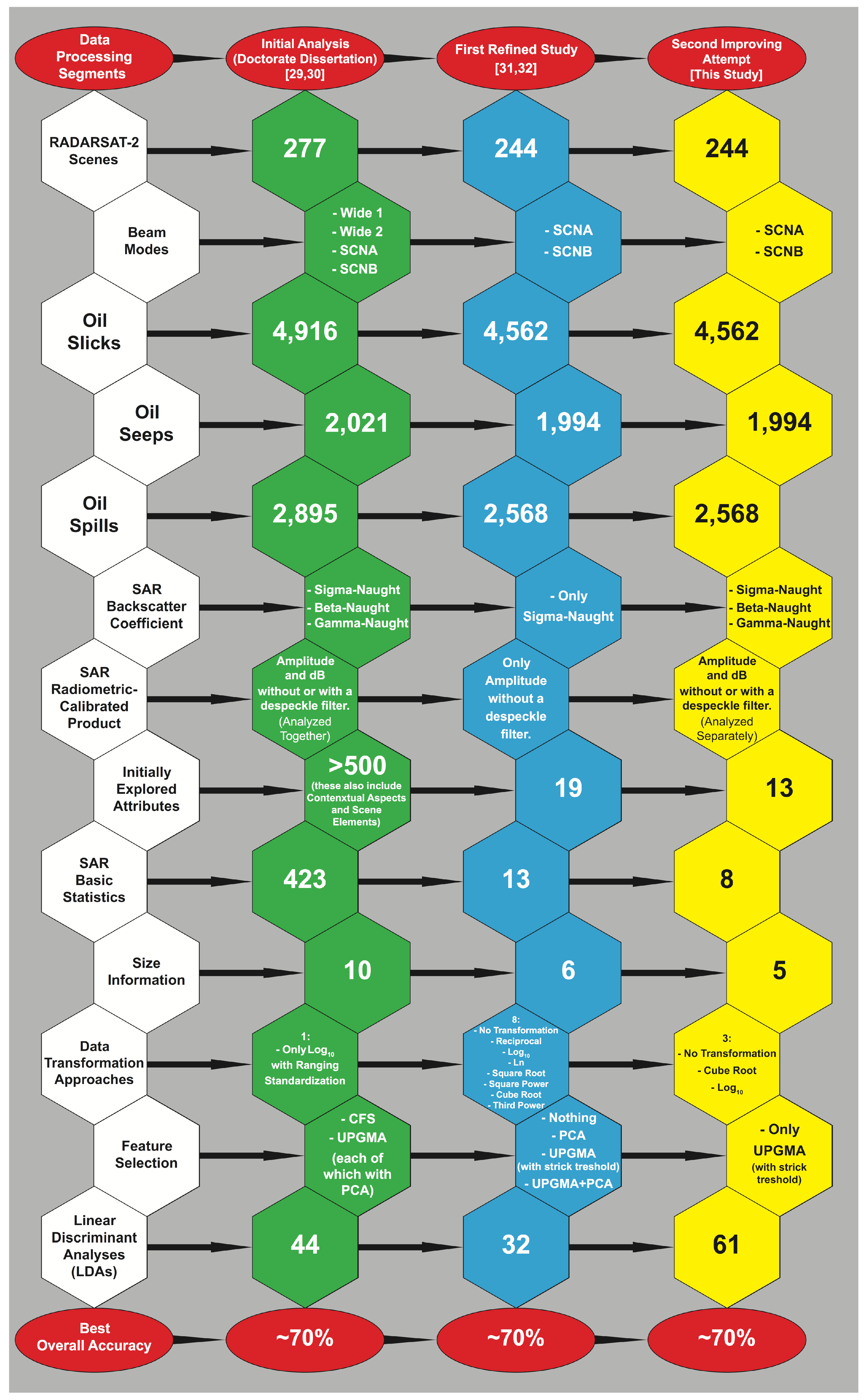
• Which SAR backscatter coefficient (i.e., sigma–naught (σ°), beta–naught (β°), and gamma–naught (γ°)) provides the most accurate seep–spill discrimination?
• Which SAR calibrated product (i.e., measures of the received radar beam given in amplitude or decibel, with or without a despeckle filter) leads to the best seep–spill discrimination?
• Which of the three tested data transformations (i.e., none, cube root, and log₁₀) leads to more effective discrimination between seeped and spilled oil?
• Which combination of attributes describing the oil-slicks’ signature (e.g., size information and SAR basic qualitative-quantitative statistics) better discriminates between the two oil-slick categories?

Our study contributes both to academic ocean remote sensing research and to practical applications in the oil and gas industry and elsewhere. We expect that approaches other than our LDA-based algorithms may also lead to improved seep–spill discrimination; however, these require further attention from the scientific community.

This manuscript adopts a customary writing structure: introduction (Section 1), methods (Section 2), results (Section 3), discussion (Section 4), and concluding remarks (Section 5). While Section 1 dwells upon our research motivations, justifications, and contributions, Section 2 presents information about the explored dataset (Section 2.1) and about a specific ongoing operational petroleum industry application currently applying our proven oil-slick remote sensing technique (Section 2.2), as well as it discloses the concepts for discriminating the oil-slick category (Section 2.3) and sets forth a description of our exploratory data analysis (Section 2.4).

2. Materials and Methods

Figure 1 depicts the study area: the oceanographically dynamic, southernmost bight of the Gulf of Mexico, Campeche Bay. Figure 2 presents the research rationale of our exploratory data analysis bridging academic research and the petroleum industry. The satellite images have been processed with PCI Geomatica (PCI Geomatics; Markham, ON, Canada). PAST (PAleontological STatistics: Oslo, Norway [42,43,44]) was used to complete the multivariate data analyses.

2.1. Dataset

One of the foremost difficulties in many ocean remote sensing studies is the availability of field information paired with concurrent satellite imagery—a good baseline training dataset is a primary prerequisite for the success of environmental analyses [45]. In this sense, we resorted to the satellite-field data put together by Pemex (Petróleos Mexicanos; Mexico City, Mexico) that carried out a decadal (2000–2012) environmental monitoring program in Campeche Bay (Figure 1). This database came from the dire necessity to survey oil slicks in the surroundings of its numerous fossil fuel facilities in this region [18,46,47,48,49]. The entire satellite database has 766 images from the Canadian C-band SAR satellites: RADARSAT-1 (482; 63%) and RADARSAT-2 (284; 37%); all scenes of the former are 8-bit HH polarized, whereas most of the latter are 16-bit VV polarized [50,51]. This multi-year data collection of SAR-observed oil slicks—14210 classified in 6202 seeps (44%) and 8008 spills (56%)—that have been identified by domain specialists and field-validated by Pemex, is comprehensively described elsewhere [29,33,34]; these authors also provide an outlook of Pemex’s monitoring system and a thorough picture of the observed slicks’ spatial–temporal distribution.

Here, our long-term exploratory data analysis explores a fraction (32%) of the entire satellite database: a total of 244 scenes from the low-cost, more numerously available RADARSAT-2 (16-bit VV), wider swath beam mode: ScanSAR Narrow—SCNA and SCNB, both having swath widths of 300 km and ground resolutions of 50 m [52]. This avoids the additional cross-comparison effects concerning technical differences of two the satellites. This dataset is the same one exploited earlier [31,32], and includes images from 2008 to 2012 that contain 4562 oil slicks; coincidently the same unbalanced proportion of the entire database: 1994 seeps (44%) and 2568 spills (56%). The experimental methodology applied to evaluate the outcomes of our LDAs uses all 4562 oil slicks for training the algorithms.

2.2. Proven Technique

The research reported here is a step in the evolution from a cutting-edge academic oil-slick remote sensing epistemology strategy to a specific ongoing operational application of the petroleum industry—Figure 2. Inside this scope, regarding the former, the initial concept and design directed at discriminating the slick categories (i.e., seeps vs. spills) using LDA applied to SAR measurements was developed by Carvalho (2015) [29]. In relation to the latter, a semi-public multinational oil and gas company (i.e., Brazilian Petroleum Corporation: Petrobras) is currently funding a research and development project—since 2018, with a five-year horizon—perhaps, to implement such an innovative oil-slick discrimination methodology to assist its strategic field operations to locate prospective offshore oil exploration frontiers in the Campos and Santos Basins, important physiographic provinces of the Brazilian Continental Margin [53,54]. Through its research headquarter, Leopoldo Américo Miguez de Mello Research and Development Centre (known as CENPES), Petrobras is jointly developing our freely-available seep–spill discrimination approach with researches at the Pontifical Catholic University of Rio de Janeiro (PUC-RJ).

2.3. Concepts for Discriminating the Oil-Slick Category

The data processing segments undergone to reach the existing expertise knowledge of discriminating seeps from spills are disclosed. A chronological outline of the published scientific literature on the subject of categorizing slicks into seeps and spills is given:

• [29,33,34] describe the dataset;
• [29,30] discuss the original exploratory multivariate data analysis—referred to as the initial exploratory analysis; and
• [31,32] present further developments of the original analysis in a more controlled fashion—referred to as the first refined study.

Collectively, these publications bring together our earlier investigations, having in common an overall accuracy of ~70% in discriminating the slick category. The current research is the second attempt at trying to improve the seep–spill discrimination, leading us to perform a more rigorous, detail-oriented approach.

2.3.1. Concept 1: SAR Signature

To cope with the seep–spill discrimination, the initial exploratory analysis used straightforward LDA-based algorithms applied to measurements of two forms of SAR signatures:

• SAR backscatter coefficients: σ°, β°, and γ° [55,56,57]; and
• SAR calibrated products: back-scattered radar beam measurements given in amplitude (amp) or in decibel (dB), both with or without the application of a despeckle filter [58].

Even though the relationship among σ°, β°, and γ° are geometrically related at the pixel level assuming the ocean to be a horizontally flat surface, the sea surface undergoes changes in height and inclination relative to the incident radar beam due to long-period waves [59]. Given that differences in sea surface heights are measured by satellite microwave altimeters (e.g., significant wave height [60,61]), we believe that such variations may influence the SAR backscatter coefficient within the oil slicks’ surface, thus affecting our ability to discriminate the slick category.

The calibrated products differ one from another mathematically, representing possible ways to influence the discrimination of seeps from spills. In fact, dB values are derived by applying a logarithm function (log₁₀) to the amplitude of the back-scattered radar beam (denoted amp) and multiplying it by a constant value (in this case: 20)—this dB transformation occurs in the pixel level. Moreover, despeckle filtering strategies also alter the value of each pixel (e.g., the Frost filter [62]).

At the outset of the initial analysis [29,30], the full SAR signature set was investigated together as one entity, then, all calibrated products (four) were analyzed together for each backscatter coefficient (three). On the other hand, only σ° amp with no despeckle filter (SIG.amp) was explored in the refined study [31,32], thus providing a firmer basis and more control in the understanding of the seep–spill categorization process.

2.3.2. Concept 2: Explored Attributes

The initial exploratory analysis experimentally choose the simpler as possible variables to represent four types of attributes: contextual aspects (33 in number; e.g., latitude, longitude, etc.), SAR scene elements (36; e.g., beam modes and incident angles), size information (10; e.g., area, perimeter, and several ratios using these fundamental morphological characteristics—e.g., perimeter/area, etc.), and SAR basic qualitative-quantitative statistics (423—including all SAR signature forms, e.g., central tendency, dispersion, etc.).

All size information ratios were identified following the literature but from studies differentiating oil (slicks) from the so-called look-alike features (e.g., low wind zones), rather than categorizing oil (seeps) from oil (spills) as in our analyses. The SAR basic statistics consist of quantities describing the received radar signal strength that are calculated with all pixels of each individual oil slick.

The knowledge evolution imparted by the initial analysis [29,30] that experimentally explored a broad set of attributes (i.e., >500 variables describing each oil slick) led to the first refined study drastically reducing the dimensionality by starting the analyses using only 19 variables that performed with comparable discrimination effectiveness [31,32]. This reduction in the number of attributes mostly refers to the elimination of: (1) contextual aspects, as their use provides an almost 100% site-specific flawless discrimination that may limit comparisons with other regions; (2) scene elements, as we only use one beam mode and do not consider incident angle variations within a given frame; (3) size information owing the same (or inverted) frequency distributions (i.e., equivalent statistical meanings); and (4) SAR basic statistics with intra-statistical correlation (i.e., highly correlated attributes), which are not suitable to be used in LDAs, because they do not bring useful information to discrimination processes [63].

The initial exploratory analysis [29,30] applied a negative value-scaling filter, whereas the first refined study [31,32] applied a minimum value-scaling filter. These linear scaling operations bring the information of each pixel to the positive domain, as the minimum value-scaling filter is applied to all pixels in oil slicks, in which the new positive value is derived by subtracting the minimum value of each oil slick from the original pixel value.

2.3.3. Concept 3: Data Transformations

The initial exploratory analysis explored a single non-linear normalization (log₁₀) and one linear standardization (Ranging). This contrasts with the first refined study in which the impact of eight non-linear transformations were tested: no transformation (x), reciprocal (1/x), logarithm base 10 (log₁₀(x)), napierian logarithm (ln(x)), square root (x^1/2), square power (x²), cube root (x^1/3), and third power (x³). This comparison revealed that cube root and log₁₀ performed superiorly than the other transformations, having similar seep–spill discrimination accuracies: overall accuracies of ~70%.

Notwithstanding the fact that the data were transformed in multiple ways to seek improvements in the discrimination process, to obtain the calibrated product in dB, log₁₀ was applied at the pixel level, whereas the data transformations, which include log₁₀, were applied to the attributes representing the entire oil slick’s surface (e.g., size information and SAR basic statistics).

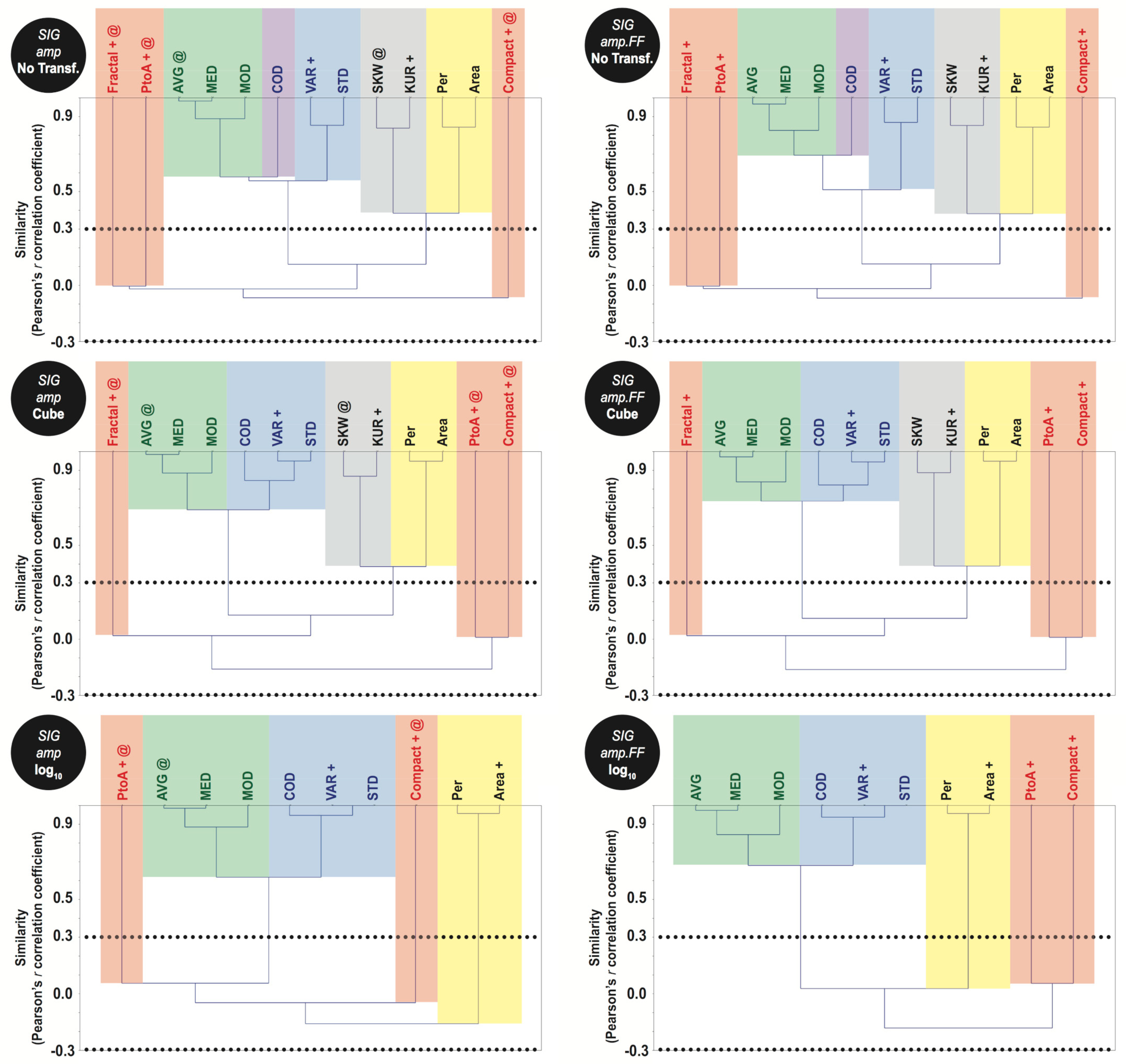
2.3.4. Concept 4: Feature Selection Methods

During the initial exploratory analysis [29,30], two feature selection methods were tested in the R-mode [64]. While dealing with large numbers of variables at the start (>500), these methods selected similar attributes:

• Correlation-Based Feature Selection (CFS): Automatic-configured routine specifying a “Merit” to evaluate inter-statistical correlations among different groups of variables using the information of the categories being discriminated [65,66].
• Unweighted Pair Group Method with Arithmetic Mean (UPGMA): Semi-automated method exploring rooted-tree diagrams (i.e., dendrograms). Its attribute selection process forms groups based on a similarity measure (e.g., Pearson’s r correlation coefficient) in which each element of the matrix undergoes a simple linear two-by-two correlation. This method is adjustable to the user’s needs as groups of correlated variables are relative to a user-defined cut-off to select them, that is, a phenon line (e.g., r = 0.5 and 0.9), which is a horizontal line draw across the dendrograms [67,68,69].

Once variables were selected with these methods, they were separately put onto an orthogonal transformation [64,69]:

• Principal Component Analysis (PCA): Linear transformation approach used to select the most relevant principal component (PC) axes. The PCs’ scores were the ones used as input to the LDA.

Conversely, during the refined study [31,32], four feature selection methods were tested:

• Do nothing—i.e., all variables were directly inserted onto the LDA;
• Using all variables straight to PCAs without passing thought the UPGMA selection;
• Same approach as used in the initial exploratory analysis [29,30] but using only the UPGMA analyses as it offers more control in the attribute selection process than the CFS. This time, the application of a stricter similarity phenon threshold (i.e., r = 0.3, instead of 0.5 or 0.9) guarantees variables are deemed to have no significant statistical correlation from one another [70]. This leads to using the values of the attributes directly to the LDA; instead of the PCs’ scores. This alternative circumvents the application of PCAs and simplifies the seep–spill discrimination process; and
• The sole and strict UPGMA cut-off but this time with PCA.

Of these four methods, the third has been reckoned to be the simplest, direct, and most efficient [31,32].

2.3.5. Concept 5: Linear Discriminant Analysis (LDA)

We have been exploring LDA-based algorithms to find a linear combination of predictors (i.e., attributes—e.g., size information and SAR basic statistics) to best separate targets (i.e., oil slicks) [64]. We deal with a classification problem of discriminating seeps from spills into mutually exclusive groups with this parametric method. The LDA is a simple, standard statistical binary classifier that produces a model whose effectiveness can be as good as more complex non-parametric regression algorithms [71,72] (i.e., machine learning techniques)—for instance, artificial neural network (ANN) or support vector machine (SVM) [28,63]. The use of such non-linear mappings to discriminate seeps from spills should be further explored.

The LDA specifies the maximum probability of an incorrect discrimination to be minimized [64]. It uses predetermined information (i.e., explored attributes) along with the a priori category membership (i.e., seep or spills). To this matter, the dependent variable (i.e., discriminant function: DF(x)), is given by the summation of all independent variables (x_n) multiplied by their weight (w_n), minus a constant offset (off), such that: DF(x) = (w₁x₁ + w₂x₂ + w_nx_n) − off. The independent variables are represented by the values of the explored attributes, whereas w_n and off are calculated by the best fit of the model [64,71,72].

The dependent variable is compared to the category membership to estimate the LDA power. To access the discrimination accuracy in our investigations, we used a two-by-two table (i.e., confusion matrix—

Table 1. Confusion matrix [73,74]. In our current research, our linear discriminant analyses (LDAs) explore a condensed two-by-two table format—refer to Table 3.

	LDA Oil Seeps	LDA Oil Spills	Known Oil Slicks
Known oil seeps	A	B	A + B
Known oil spills	C	D	C + D
LDA oil slicks	A + C	B + D	A + B + C + D

See Table 2 for A, B, C, and D, as well as for associated metrics [75,76,77].

[73,74]) and its associated standard statistical metrics—

Table 2. List of statistical standard metrics associated with the confusion matrix [75,76,77]. See Table 1 for A, B, C, and D. Bold indicates relevant metrics explored herein—refer to Table 3.

Diagonal of Table 1	A	=	Correctly identified oil seeps
	D	=	Correctly identified oil spills
	A + D	=	Correctly identified oil slicks
Off-Diagonal of Table 1	C	=	Misidentified oil seeps
	B	=	Misidentified oil spills
	C + B	=	Misidentified oil slicks
A + B + C + D		=	Known oil slicks (i.e., 4562)
Horizontal Analysis of Table 1	A + B	=	Known oil seeps (i.e., 1994)
	C + D	=	Known oil spills (i.e., 2568)
	A/(A + B)	=	Sensitivity
	D/(C + D)	=	Specificity
	B/(A + B)	=	False negative
	C/(C + D)	=	False positive
Vertical Analysis of Table 1	A + C	=	LDA classified oil seeps
	B + D	=	LDA classified oil spills
	A/(A + C)	=	Positive predictive value
	D/(B + D)	=	Negative predictive value
	C/(A + C)	=	Inverse of the positive predictive value
	B/(B + D)	=	Inverse of the negative predictive value
(A + D)/(A + B + C + D)		=	Overall accuracy

[75,76,77]. At present, best overall accuracies are about 70%, obtained from the analyses of several dataset combinations: 44 (initial analysis [29,30]) and 32 (first study [31,32]). The LDA-based algorithms were trained with all 4562 oil-slick samples.

2.4. Exploratory Data Analysis

Even though our current research follows an equivalent pattern as before (see Section 2.3), we take advantage of our previously acquired understanding [29,30,31,32,33,34] to reorganize the blueprint of our exploratory data analysis (Figure 2) into a more rigorous detail-oriented scheme:

• SAR Signature: To verify which combination of SAR backscatter coefficients with SAR calibrated products provides the finest discrimination accuracy, we separately perform a complete analysis exploring the full SAR signature set (12)—i.e., SIG.amp, SIG.amp.FF, SIG.dB, SIG.dB.FF, BET.amp, BET.amp.FF, BET.dB, BET.dB.FF, GAM.amp, GAM.amp.FF, GAM.dB, and GAM.dB.FF; respectively for σ°, β°, and γ°, given in amp and in dB, with or without a despeckle filter (FF; for Frost filter [62]). This differs from the initial exploratory analysis that analyzed all calibrated products together for each backscatter coefficient [29,30].
• Explored Attributes: We apply the minimum value-scaling filter, and because we also intend to reduce dimensionality, histograms and correlation matrices are examined in an attempt to reduce the number of variables included in our analyses.
• Data Transformations: To evaluate the impact of the two best non-linear transformations found in the first refined study (i.e., cube root and log₁₀) we compare them with the original data with no transformation.
• Feature Selection Methods: We also avoid PCAs and solely use dendrogram analyses with the strict phenon threshold (r = 0.3), as indicated by the results of the first refined study [31,32].
• Linear Discriminant Analysis (LDA): Our LDA-based algorithms involve an analysis of a number of combinations of the three backscatter coefficients, each of which is calculated from the four calibrated products and the three data transformations (36 instances). We also investigate the standalone use of the size information with the tested transformations (3 instances); these are referred to as size only. We also consider 22 extra combinations using several of the main 39–data instances analyzed together—“hybrid schemes”—resembling those used by [75,76]. Therefore, we investigate 61–dataset combinations. To this matter, due to the outsized amount of two-by-two tables analyzed in our current research, these dataset combinations are evaluated based on

  Table 3. Condensed confusion matrix form (i.e., Table 1) showing the statistical metrics (i.e., Table 2) explored herein to evaluate our linear discriminant analysis (LDA) algorithms.

  Oil Seeps		Oil Spills		Oil Slicks
  Correctly Identified oil seeps	Sensitivity	Correctly Identified oil spills	Specificity	Correctly Identified oil slicks	Overall accuracy
  	Positive predictive value		Negative predictive value

  , a condensed form of the classic confusion matrix design. We use this abridged-table format to simplify the visualization of our outcomes. The exploratory nature of our analyses focuses on exploring all 4562 oil slicks to train our LDA-based algorithms.

3. Results

The data processing segments aimed at discriminating the slick category using LDA-based algorithms are summarized in Figure 3.

3.1. Explored Attributes

We removed certain attributes at the start of our analyses using three major correlation matrices: one for each data transformation, accounting for the three backscatter coefficients and four calibrated products, accounting for the 19 variables from the first refined study [31,32]. Accordingly, herein, we simply explore the information of 13 variables, thus reducing the dimensionality of the problem in relation to our earlier investigations (Figure 3). This set of variables are collectively referred to as the oil-slicks’ signature:

• Area (Area);
• Perimeter (Per);
• Ratio between Per and Area (PtoA [78]);
• Compact index (4.π.Area/Per² [28]);
• Fractal index (2.ln(Per/4)/ln(Area) [79]);
• Average (AVG);
• Median (MED);
• Mode (MOD);
• Standard deviation (STD);
• Variance (VAR);
• Coefficient of dispersion (COD: the third interquartile minus the first, divided by their sum);
• Skewness (SKW); and
• Kurtosis (KUR).

The first five correspond to the size information and the next eight are the SAR basic qualitative-quantitative statistics. The latter are divided in: central tendencies (AVG, MED, and MOD), measures of dispersion (STD, VAR, and COD), and pixel distribution metrics (SKW and KUR).

An imperative information is that when log₁₀ is applied, only 10 variables are accounted, as Fractal, SKW, and KUR have negative values preventing their use.

3.2. Feature Selection Methods

The UPGMA dendrograms for the twelve σ° instances are shown in Figure 4 (SIG.amp and SIG.amp.FF) and Figure 5 (SIG.dB and SIG.dB.FF); those for β° and γ° are very similar to those of σ° independent of data transformation. Using the strict threshold (dotted horizontal phenon similarity line: r = 0.3), we select one variable (+) from each resulting group. Groups of similar (correlated) variables are color-coded to facilitate visual interpretation.

The central tendency (green) and dispersion (blue) variables group between each other, and together they form a single group (Figure 4: amp and amp.FF). The behavior of the central tendency and dispersion counterparts is disturbed when variables are dB transformed (purple), such that KUR becomes part of this group once no transformation or cube root occur (Figure 5: left); though, this is not observed in dB.FF (Figure 5: right). COD also stands out from grouping with the other dispersion variables in dB and dB.FF (Figure 5: purple), as well as in the original data with no transformation (Figure 4: amp and amp.FF). From this larger green-blue group VAR is selected.

The pixel distribution (gray) pairs with the twosome of Area and Per (yellow) while in amp and amp.FF (Figure 4). This pixel distribution behavior breaks down in dB and dB.FF (Figure 5: left and right). From this gray-yellow larger group KUR is selected.

The size information ratios (red) do not show correlation with any other attribute (r ~0.0). As such, they are selected when present—i.e., no transformation and cube root. They tend to assemble (Figure 4), but sometimes this do not hold true (Figure 5: purple).

A distinctive characteristic is revealed when analyzing dB (cube and log₁₀) and dB.FF (log₁₀)—see (*) in Figure 5. All variables possess significant statistical correlation—i.e., their relationships exceed below the phenon similarity strict threshold of r = −0.3. Although no variable should have been selected, to avoid such disrupting action we selected comparable attributes with the other analyses to perform a second round of dendrogram analysis only with these variables (+). Indeed, their selection shows no intra-correlation—this is also supported by the major correlation matrices.

Table 4. Uncorrelated variables (+) selected with the unweighted pair group method with arithmetic mean (UPGMA) dendrogram analyses for sigma–naught (SIG), beta–naught (BET), and gamma–naught (GAM), each of which calculated from four SAR calibrated products (received radar beam given in amplitude (amp) or decibel (dB), with or without a despeckle filter, i.e., FF: for Frost filter [62]), for the tested non-linear transformations: none (left), cube root (middle), and log₁₀ (right). The twelve SIG instances (shown in bold) have their dendrograms depicted in Figure 4 and Figure 5. See Section 3.1 for explored variables. Oil-slicks’ signature: size information (1–5) and SAR basic qualitative-quantitative statistics (6–13). Basic morphological features: 1 and 2. Basic morphological ratios: 3–5. Central tendencies: 6–8. Dispersion measures: 9–11. Pixel distribution metrics: 12 and 13.

(@) Explored in the first refined study [31,32]. (*) Second round of UPGMA analysis required; see the text for explanation and Figure 5 for visualization. (o) Variables not accounted for (see Section 3.1).

lists the UPGMA uncorrelated variables selected for each of the main 39–data instances. Most combinations (26) include the three size information ratios: PtoA, Compact, and Fractal – only in the log-transformed ones (13) whereby Fractal is not present as it accounts for negative values. Some combinations (12) also have Area selected, i.e., dB and dB.FF with no transformation and log₁₀. Of the 36–data instances exploring SAR basic statistics, VAR is selected in all of them. In almost all (18) not- and cube-transformed combinations, KUR is chosen, and in only three instances SKW is selected in its place: dB with no transformation. Thus, usually (in 15 instances), we have five attributes as the most frequently used in the LDA-based algorithms: PtoA, Compact, Fractal, VAR, and KUR; independent of SAR backscatter coefficient, SAR calibrated product, or data transformation. The number of selected attributes varies from two to six (Table 4):

• Two variables are selected in only one instance: size only log-transformed (1).
• Three attributes are chosen in eight instances: size only with no transformation and log₁₀ (2), and dB and dB.FF log-transformed (6).
• Four variables are selected in nine instances: cube-dB (3), and amp and amp.FF log-transformed (6).
• Five attributes are accounted in the largest set of instances (fifteen): amp and amp.FF with no transformation (6), and all cube-transformed ones (9) not including dB.
• Six variables are selected in six instances: when no transformation is applied to dB and dB.FF (6).

Comparing our SIG.amp dendrograms (Figure 4: left panels) with those from the refined study [31,32], the removal of six attributes to start the analysis (13 against 19) causes only a minor impact on the similarity of the retained variables, and yields small changes in the in-group configuration using the same strict similarity cut-off (r = 0.3). The main exception occurs in the log-transformation Figure 4 (bottom left), in which the size information similarities are altered, but not influencing the grouping of the variables, nor the selected features. The selection of uncorrelated attributes only varies between this research and prior approach [31,32] because we opt to select different variables within the formed groups (i.e., VAR instead of AVG, and KUR in lieu of SKW).

3.3. Linear Discriminant Analysis (LDA)

Because our analyses produced many two-by-two tables, we evoke an abridgment of the classic confusion matrix (Table 3) to display the LDA results of the main 39–data instances into a single table, as hierarchized in

Table 5. Outcomes of our linear discriminant analyses (LDAs). Refer to Table 3 for explanations.

Hierarchy	Data Transformation	Oil-Slicks’ Signature		Oil Seeps		Oil Spills		Oil Slicks
1	log10	Gamma-naught	dB	1293	64.84%	1848	71.96%	3141	68.85%
					64.23%		72.50%
2	log10	Beta-naught	dB	1292	64.79%	1848	71.96%	3140	68.83%
					64.21%		72.47%
3	log10	Sigma-naught	dB	1292	64.79%	1845	71.85%	3137	68.76%
					64.12%		72.44%
4	log10	Gamma-naught	dB.FF	1293	64.84%	1842	71.73%	3135	68.72%
					64.04%		72.43%
5	log10	Sigma-naught	dB.FF	1292	64.79%	1838	71.57%	3130	68.61%
					63.90%		72.36%
6	log10	Size only		1288	64.59%	1841	71.69%	3129	68.59%
					63.92%		72.28%
7	log10	Beta-naught	dB.FF	1288	64.59%	1840	71.65%	3128	68.57%
					63.89%		72.27%
8	log10	Sigma-naught	amp.FF	1321	66.25%	1806	70.33%	3127	68.54%
					63.42%		72.85%
9	log10	Sigma-naught	amp	1323	66.35%	1803	70.21%	3126	68.52%
					63.36%		72.88%
10	log10	Beta-naught	amp	1324	66.40%	1800	70.09%	3123	68.48%
					63.29%		72.87%
11	log10	Gamma-naught	amp	1320	66.20%	1803	70.21%	3124	68.46%
					63.31%		72.79%
12	log10	Gamma-naught	amp.FF	1320	66.20%	1802	70.17%	3122	68.44%
					63.28%		72.78%
13	log10	Beta-naught	amp.FF	1320	66.20%	1799	70.05%	3119	68.37%
					63.19%		72.75%
14	Cube root	Gamma-naught	amp.FF	1409	70.66%	1709	66.55%	3118	68.35%
					62.13%		74.50%
15	Cube root	Sigma-naught	amp.FF	1410	70.71%	1706	66.43%	3116	68.30%
					62.06%		74.50%
16	Cube root	Gamma-naught	dB.FF	1384	69.41%	1729	67.33%	3113	68.24%
					62.26%		73.92%
17	Cube root	Beta-naught	dB	1393	69.86%	1720	66.98%	3113	68.24%
					62.16%		74.11%
18	Cube root	Beta-naught	amp.FF	1409	70.66%	1703	66.32%	3112	68.22%
					61.96%		74.43%
19	Cube root	Gamma-naught	dB	1391	69.76%	1719	66.94%	3110	68.17%
					62.10%		74.03%
20	Cube root	Sigma-naught	dB.FF	1378	69.11%	1730	67.37%	3108	68.13%
					62.18%		73.74%
21	Cube root	Beta-naught	dB.FF	1385	69.46%	1722	67.06%	3107	68.11%
					62.08%		73.87%
22	Cube root	Sigma-naught	dB	1390	69.70%	1719	66.90%	3109	68.10%
					62.10%		74.00%
23	Cube root	Sigma-naught	amp	1405	70.46%	1701	66.24%	3106	68.08%
					61.84%		74.28%
24	Cube root	Beta-naught	amp	1402	70.31%	1699	66.16%	3101	67.98%
					61.73%		74.16%
25	Cube root	Gamma-naught	amp	1404	70.41%	1697	66.08%	3101	67.98%
					61.71%		74.20%
26	Cube root	Size only		1400	70.21%	1685	65.62%	3085	67.62%
					61.71%		73.94%
27	No transformation	Gamma-naught	dB.FF	1563	78.39%	1433	55.80%	2996	65.67%
					57.93%		76.88%
28	No transformation	Beta-naught	dB.FF	1560	78.23%	1426	55.53%	2986	65.45%
					57.74%		76.67%
29	No transformation	Sigma-naught	dB.FF	1557	78.08%	1427	55.57%	2984	65.41%
					57.71%		76.56%
30	No transformation	Gamma-naught	dB	1559	78.18%	1410	57.91%	2969	65.08%
					57.38%		76.42%
31	No transformation	Sigma-naught	dB	1555	77.98%	1407	54.79%	2962	64.93%
					57.25%		76.22%
32	No transformation	Beta-naught	dB	1554	77.93%	1403	54.63%	2957	64.82%
					57.15%		76.13%
33	No transformation	Gamma-naught	amp.FF	1580	79.24%	1354	52.73%	2934	64.31%
					56.55%		76.58%
34	No transformation	Gamma-naught	amp	1580	79.24%	1353	52.69%	2933	64.29%
					56.23%		76.57%
35	No transformation	Sigma-naught	amp.FF	1580	79.24%	1353	52.69%	2933	64.29%
					56.53%		76.57%
36	No transformation	Sigma-naught	amp	1579	79.19%	1352	52.65%	2931	64.25%
					56.49%		76.51%
37	No transformation	Beta-naught	amp.FF	1580	79.24%	1351	52.61%	2931	64.25%
					56.49%		76.54%
38	No transformation	Beta-naught	amp	1580	79.24%	1347	52.45%	2927	64.16%
					56.41%		76.49%
39	No transformation	Size only		1574	78.94%	1341	52.22%	2915	63.90%
					56.19%		76.15%

. These hierarchies are based on the analyses of the overall accuracy and associated metrics imparted by Table 3. The seep–spill discrimination accuracies of the 22 hybrid schemes (data not shown) fall within the accuracy limits of the main 39–data instances. Therefore, we focus on the information in Table 5, as it conveys the LDA outcomes for all 61–data combinations. These have been obtained after training the algorithms with all 4562 oil slicks. Other metrics can also evaluate the performance of discrimination algorithms (e.g., Cohen’s kappa coefficient); however, we choose those in Table 3 as our approach has an operational focus.

The discretization interval of our LDAs is 0.02%. This resolution limit represents the smallest detectable difference of the explored dataset—i.e., one misidentified slick: 1/4561. The worst overall accuracy is observed with the original data of the size only combination: 63.90% (2915 slicks correctly identified: 1574 seeps and 1341 spill). The most effective accuracy is observed with the log₁₀ GAM.dB combination: 68.85% (3141 slicks correctly identified: 1293 seeps and 1848 spill).

The first important aspect in Table 5 is that key hierarchy–accuracy groupings are formed. There are three major blocks influenced by the data transformations. Some combinations are deemed to perform better than others—top-down: log₁₀, cube root, and no transformation. Within these major blocks, the SAR calibrated products are grouped forming minor blocks; usually dB (with or without FF) summits most effectively (except in cube root, where amp.FF reaches better accuracy). The SAR backscatter coefficients are distributed within these minor blocks, where γ° tends to have better accuracies.

Quantifying the hierarchy misidentification of the data transformation blocks (Table 5), we observe that the log₁₀ combinations have the best overall accuracy (GAM.dB: 68.85%). The log₁₀ combinations have the best oil-spill identification rate (1848 GAM.dB and BET.dB) but correctly detect the least amount of oil seeps (1288: BET.dB.FF). On the other hand, the not-transformed original data are inversely propositional to log₁₀—i.e., have a poorer overall accuracy (size only: 63.90%) being the worst one to identify oil spills (1341: size only) but the best one to correctly identify oil seeps (1580: GAM and BET, both with amp and amp.FF).

Table 6. Statistics summary of our linear discriminant analyses (LDAs) based on the major blocks of data transformations (log₁₀, cube root, none) from the 39–data instances hierarchized in Table 5.

All Three Transformations	Oil Seeps	Sensitivity	Oil Spills	Specificity	Oil Slicks	Overall Accuracy
Maximum	1580	79.24%	1848	71.96%	3141	68.85%
Minimum	1288	64.59%	1341	52.22%	2915	63.90%
Average	1424	71.40%	1639	63.81%	3063	67.13%
Range	292		507		226
log10	Oil Seeps	Sensitivity	Oil Spills	Specificity	Oil Slicks	Overall Accuracy
Maximum	1324	66.40%	1848	71.96%	3141	68.85%
Minimum	1288	64.59%	1799	70.05%	3119	68.37%
Average	1305	65.45%	1824	71.04%	3129	68.60%
Range	36		49		22
Cube root	Oil Seeps	Sensitivity	Oil Spills	Specificity	Oil Slicks	Overall Accuracy
Maximum	1410	70.71%	1730	67.37%	3118	68.35%
Minimum	1378	69.11%	1685	65.62%	3085	67.62%
Average	1397	70.06%	1711	66.62%	3108	68.12%
Range	32		45		33
No Transformation	Oil Seeps	Sensitivity	Oil Spills	Specificity	Oil Slicks	Overall Accuracy
Maximum	1580	79.24%	1433	55.80%	2996	65.67%
Minimum	1554	77.93%	1341	52.22%	2915	63.90%
Average	1569	78.70%	1381	53.79%	2951	64.68%
Range	26		92		81

presents a summary of the seep–spill discrimination statistics regarding the transformation blocks. Even though the log-transformed combinations (GAM.dB: 68.85%) outperform the cube-combinations (GAM.amp.FF: 68.35%), the latter show more balanced seep–spill correct identification capabilities. The unbalanced seep (spill) log₁₀ dispersal is: min 1288 (1799) and max 1324 (1848). The balanced min seep (spill) correct cube root identification is 1378 (1685) and its max seep (spill) correct detection is 1410 (1730). Equivalently, the best original not-transformed data also have a fairly balanced seep (spill) identification rate; however, with less oil slicks correctly identified (GAM.dB.FF: 65.67%)—min 1554 (1341) and max 1580 (1433).

From Table 6 we also note the range (226) of the three transformations: oil slicks correctly identified varied from 3141 (log₁₀ GAM.dB) to as low as 2915 (not-transformed size only). While the oil seeps’ range (292) varied from 1580 (no transformation: GAM and BET, both with amp and amp.FF) to 1288 (log₁₀ BET.dB.FF), the oil spills’ range is larger (507) and goes from 1848 (log₁₀ GAM.dB and BET.dB) to 1341 (not-transformed size only). Some equivalence exists between the seep, spill, and slick ranges of the log₁₀ (36, 49, and 22) and cube (32, 45, and 33) combinations. The original data ranges are: 26 (seeps), 92 (spills), and 81 (slicks).

Table 6 also shows that, on average, the overall accuracy of all oil slicks is 67.13%. If considering the average of the log₁₀ (68.60%) and cube (68.12%) combinations, these have similar discrimination performances, though, as pointed out, the latter surpass the former with its more balanced seep–spill discrimination. The original data with no transformation had the lowest discrimination overall accuracy average: 64.68%.

The second remarkable aspect observed in Table 5 is related to the hierarchy-accuracy grouping of the original not-transformed data. None of its 13 data instances are valid. They had very low (<60%) specificity (i.e., of the a priori know spills, how many the LDA identifies correctly?) and positive predictive values (i.e., of the LDA-identified seeps, how many are actually seeps?). This means that the data needs to be normalized to achieve success in discriminating the oil-slick category using our linear approach.

The third noteworthy aspect observed in Table 5 concerns the choice of variables, i.e., oil-slicks’ signature: size information and SAR basic qualitative-quantitative statistics—see (@) in Table 4. To this matter, we call a comparison between our current research (Table 5) and the first refined study (

Table 7. Outcomes of the linear discriminant analyses (LDAs) from the first refined study [31,32]. Top: oil-slicks’ signature (SAR signature: sigma–naught with no despeckle filter—SIG.amp). Bottom: size information (size only: PtoA and Compact). See also Table 1, Table 2, Table 3, Table 4 and Table 5.

Hierarchy	Data Transformations	Oil-Slicks’ Signature	Oil Seeps		Oil Spills		Oil Slicks
1	log10	SIG.amp	1296	64.99%	1829	71.22%	3125	68.50%
				63.69%		72.38%
2	Cube root	SIG.amp	1407	70.56%	1711	66.63%	3118	68.35%
				62.15%		74.46%
3	No Transformation	SIG.amp	1570	78.74%	1344	52.34%	2914	63.88%
				56.19%		76.02%
Hierarchy	Data Transformations	Size Information	Oil Seeps		Oil Spills		Oil Slicks
1	log10	PtoA and Compact	1288	64.59%	1841	71.69%	3129	68.59%
				63.92%		72.28%
1	Cube root	PtoA and Compact	1417	71.06%	1667	64.91%	3084	67.60%
				61.13%		74.29%
3	No Transformation	PtoA and Compact	1575	78.99%	1338	52.10%	2913	63.85%
				56.15%		76.15%

). Even though the SAR basic statistics we select now (SIG.amp: VAR and KUR) are different from the ones of the refined study (SIG.amp: AVG and SKW), there is not much change in the discrimination power between the two analyses. This is independent of the way the data is transformed, for instance, SIG.amp: log₁₀ (68.52% against 68.50%), cube (68.08% against 68.35%), and no transformation (64.25% against 63.88%), respectively, for our current research and the first refined study [31,32].

The same holds true when we verify the size only combinations (see (@) in Table 4) between now (Table 5) and then (Table 7). In our current research we account for three size information variables (Table 4: PtoA, Compact, and Fractal), whereas in the refined study only two were used (Table 7: PtoA and Compact). Again, these discrimination outcomes are quite close, with size only log₁₀ categorizing exactly the same oil slicks in our current research (Table 5) and in the refined study (Table 7): log₁₀ (68.59% against 68.59%), cube (67.62% against 67.60%), and no transformation (63.90% against 63.85%), respectively, for our current research and the first refined study [31,32].

We also note in Table 7 that the analyses of the size and SAR signatures together (i.e., SIG.amp) do not impact the outcomes much. For the log-transformed discrimination accuracy, in fact, it worsens the overall accuracy: 68.59% (size only) and 68.50% (size and SAR together). However, it does impact the cube-transformed, improving its seep–spill categorization capacity: 67.60% and 68.35%, respectively. For the original not-transformed data, only one oil slick is differently classified. Similar patterns happen in our current analysis (Table 5).

The accuracy behavior of the oil-slicks’ signature (size and SAR), on the other hand, is actually slightly different once we account for the other SAR backscatter coefficients and SAR calibrated products (Table 5). In the relation to the data transformations, size only has the poorer performance of all instances in both no transformation (63.90%) and cube root (67.62%), but when the SAR signature is taken into account we obtain improved accuracies: no transformation (GAM.dB.FF: 65.67%) and cube root (GAM.amp.FF: 68.35%). Likewise, when we compare the log₁₀ instances size information without (size only: 68.59%) and with the SAR signature (GAM.dB: 65.85%), there is also an improvement; smaller though.

4. Discussion

We have focused on giving more rigor to our detail-oriented seep–spill discrimination (Section 2.4). This second data-driven effort to try to improve the slick category categorization has benefited from the findings of our earlier investigations (Section 2.3). The study presented herein bridges our academic oil-slick remote sensing investigation and a specific ongoing operational application of the petroleum industry (Section 2.2). Because the seep–spill discrimination research is at an early stage of development, there is a continuing necessity to devote scientific attention to it. As this need tends to increase with time, reliable means of improving the capabilities to differentiate the slick category are required [29,30,31,32,33,34]. There is a lack of information in the literature concerning this topic; see [29] and references therein. There have been a number of review papers, but these have focused on the detection and characterization of oil slicks in satellite remotely sensed images, and have not addressed the categorization of slicks into seeps or spills—e.g., [80].

We recognize our linear technique exploring LDA-based algorithms is one of several possible approaches leading to improving seep–spill discrimination skills. So far, our approach has been to explore simple methods before moving on to more complex ones. Other multivariate data analyses (e.g., cubist or random forest) may also lead to better slick category discrimination. Nevertheless, further studies are needed to investigate whether these approaches can be more successful in discriminating seeps from spills than our reported results: sound overall accuracy of about 70% and practical levels of the associated standard statistical metrics—e.g., ~80% of sensitivity, ~75% of specificity, ~65% and ~75% of positive and negative predictive values, respectively. These have been reached while evaluating our algorithms using all 4562 oil slicks for training. We look forward to see the exploratory data analysis promoted by our study motivating other scholars to investigate alternative methods to discriminate the categories of oil slicks at the sea surface.

The slick category of our earlier investigations occurred with practical overall accuracy levels of ~70% [29,30,31,32]. This was found when starting the analyses with different sets of variables (>500 in [29,30] and 19 in [31,32]) and selecting uncorrelated attributes in two different ways: CFS and the UPGMA dendrograms both together with PCA in [29,30], and the simple use of a stricter UPGMA phenon cut-off but without PCA in [31,32]. Notwithstanding the best seep–spill discrimination power of our current approach being comparable to our previous investigations (~70%), we have improved it in the sense that our LDA-based efficiency is improved as we started the analysis with only 13 variables, instead of >500 [29,30] or 19 [31,32] as before (Figure 3). To this matter, the outcomes of our simple LDA approaches can guide the selection of variables to be possibly used in more complex analyses. In fact, the possibility to explore fewer variables is indeed an advantage to any eventual operational use of our seep–spill discrimination strategy.

Regarding the UPGMA dendrograms (Figure 4 and Figure 5), we observe that the SAR basic statistics variables exhibit significant statistical correlation and group among themselves: the green-blue group. The pixel distribution metrics and the Area-Per pair also have significant statistical correlation: the gray-yellow group. From these two larger groups we selected VAR and KUR, while in the first refined study we chose AVG and SKW [31,32]. This difference is rooted in the analysis of the major correlation matrices that show the former pair has less correlation than the latter with all other variables in all 39–data instances. As before [31,32], the three uncorrelated size information ratios (red groups) have also been selected

Our discrimination accuracy results are based on the analysis of the overall accuracy associated with other standard statistical metrics (e.g., sensitivity, specificity, positive and negative predictive values; Table 3). The outcomes of several dataset combinations are presented in a single table (i.e., Table 5), from which three remarkable results can be highlighted:

• Three hierarchy-accuracy groups are formed, ruled by data transformation: log₁₀, cube root, and no transformation. While the SAR calibrated products influence a second grouping within the data transformation (dB owing a superior performance), a third grouping is formed within the second but accounting for the SAR backscatter coefficients (better accuracies are found with γ°);
• Even though the LDAs of the not-transformed original data have a good overall accuracy (GAM.dB.FF: 65.67%), their specificity and positive predictive values of ~50% prevent them from discriminating successfully between seeps and spills. This follows from the fact that normal distributions are a fundamental assumption of the LDA method [64,71,72]; and
• The combination of size information and SAR basic statistics variables is more successful in categorizing slicks into seeps or spills. However, a comparison of our current results with those of the first refined study (Table 7) indicates that the choice of different variables within these two types of attributes (i.e., oil-slicks’ size and SAR information) produces small changes in the discrimination power—e.g., log₁₀ SIG.amp (68.52% (only size with VAR and KUR) against 68.50% (only size with AVG and SKW)) or only size cube-transformed information (67.62% (PtoA, Compact, and Fractal) against 67.60% (PtoA and Compact only)).

The size only information has been accounted for herein, but not SAR only (Table 4). This comes from the fact that the first refined study revealed that if the size information is removed from the analysis, the LDA is ineffectual to categorize between seeps and spills [31,32]. This means that the sole use of the selected SAR basic qualitative-quantitative statistics does not achieve successful discrimination accuracies. Perhaps, the use of other variables may show different results though.

After the completion of our analyses, and the verification of the strong relationship among σ°, β°, and γ°, we come to conclude that our assumption that changes in the sea surface height associated with the variation would influence in the seep–spill discrimination is not valid. Even though we have not measured sea surface heights, our dataset spans for five years and accounted for a large variety of sea elevations—e.g., flat ocean conditions to long-period waves.

Recommendations for Future Work

If one is to consider an expansion of the seep–spill discrimination developed throughout our investigations, we suggest, besides categorizing the oil-slick category, the investigation of the categories’ classes or the type of oil, corresponding to Bentz’s Dissertation [28]. This means that, within the oil seep category, one can possibly use LDAs to separate different seepage clusters. Analogously, among the oil spills, the LDAs can be directed at differentiating the oil from different offshore oil and gas facilities.

Another matter of interest is the application of our linear methodology (i.e., LDA-based algorithm) to a dataset containing oil (slicks) and non-oil targets (i.e., radar false targets; e.g., low wind or upwelling zones) in a similar fashion as accomplished by [28]. However, she used ANN, SVM, etc., to differentiate the on-water oil (spills) from look-alike features.

An improvement to our seep–spill discrimination process could be the use of other variables to start the analysis. We suggest exploring the dynamic fractal [81], ratios accounting for the SAR signals inside and outside of the oil slicks to standardize for the wind influence [28], gapped pixel space from transect lines through the oil slicks [82], etc. These new attributes could bring further information to our capacity to differentiate the slick category. Their statistical correlation with the oil-slick size and SAR information explored in our analyses may not be significant, meaning they could improve our LDA-based algorithm’s accuracy.

Even though we meticulously and systematically analyzed all details of our exploratory data analysis, searching for improvements in the categorization of oil (slicks) into oil (seeps) and oil (spills) with a linear multivariate data analysis technique, it may be that the LDA approaches have reached their discrimination limits (i.e., ~70% of overall accuracy) while using this multi-year satellite-field baseline training dataset. Because we reached similar effectiveness with fewer attributes in relation to our previous findings [29,30,31,32], we suggest that other non-linear methods—for instance, cubist or random forest, or even other variants such as ANN or SVM [28,63,71,72]—should be further investigated to attempt to improve on our oil-slick discrimination approach using satellite SAR measurements.

We have demonstrated that non-linear transformations cause the largest impact on the success of the seep–spill categorization (Table 5). However, so far, we only have explored the simultaneous application of the same data transformations to all variables per LDA-based algorithm (i.e., log₁₀ to Area and to Per or cube root to Area and to Per, etc.). As such, another subject that we believe can further improve the discrimination power is to apply different non-linear transformations to different variables on the same LDA algorithm—e.g., log₁₀ to Area together with cube root to Per.

5. Conclusions

We addressed a scientific problem that has also been the focus of our earlier investigations (i.e., the initial exploratory analysis [29,30] and the first refined study [31,32]) to a transition to the petroleum industry’s operational application—i.e., the use of simple, mathematically-robust linear discriminant analysis (LDA) applied to SAR measurements to discriminate the oil-slick category (oil seeps vs. oil spills). This need continues to increase with time, as new offshore fossil fuel discoveries continue to be made, but with the requirement to assist ecological monitoring and response. In fact, the Brazilian Petroleum Corporation (Petrobras) is currently exploring our proven seep–spill discrimination methodology.

Our exploratory data analysis has focused on oil-slick category discrimination exploiting different SAR backscatter coefficients (i.e., sigma–naught (σ°), beta–naught (β°), and gamma–naught (γ°)) calculated from various SAR calibrated products (i.e., amplitude (amp) or decibel (dB) measures of the back-scattered radar beam, with or without a despeckle filter (FF; for Frost filter [62])) applied to three data transformations (none, cube root, and log₁₀). This resulted in 61–data combinations using several oil-slicks’ signature (i.e., size information and SAR basic qualitative-quantitative statistics). The worst overall accuracy of all is found with the original data of the size only combination (63.90%), whereas the best one is the log-transformed GAM.dB (68.85%).

We explore 244 RADARSAR-2 images containing 4562 slicks (1994 seeps and 2568 spills) observed in Campeche Bay, Gulf of Mexico, to address our four scientific questions:

• Although the three backscatter coefficients have similar success at categorizing seeped and spilled oil (independently of the applied calibrated product or data transformation), γ° is somewhat superior.
• The discrimination power of the four calibrated products is rather independent of backscatter coefficient but varies to some extent within data transformation. When log₁₀ is applied, dB (68.85%: GAM) is followed by dB.FF (68.72%: GAM) and by two amp forms. A baffling pecking order is observed with cube root, but even though it lacks a defined hierarchy pattern, amp.FF reaches better accuracy levels (68.35%: GAM) and amp the lowest (67.98%: GAM). With the not-transformed original data, dB.FF effectiveness is followed by dB, then by the two amp forms with no definite pattern; however, these have little practical meaning—see point 3 below.
• The data transformation exerts the most influence over the seep–spill discrimination, dictating the performance of our optimal linear models. Among the tested ones, the highest overall accuracy is the log-transformed (68.85%: GAM.dB), though the cube root has slightly more balanced seep–spill discrimination capabilities and is as successful: 68.35% (GAM.amp.FF). If the data is not normalized, the top overall accuracy is 65.67% (GAM.dB.FF); nevertheless, its LDAs are incapable of separating seeps from spills, as its specificity and positive predictive values are void (~50%).
• Concerning the use of different attributes describing the oil-slicks’ signature, a comparison with the first refined study (SIG.amp) demonstrates that even though different size and SAR signatures have been used between both of our investigations (AVG and SKW against VAR and KUR; and PtoA and Compact against PtoA, Compact, and Fractal, respectively, for the refined study and our research), the discrimination improvement is disappointingly small. Although, there is an improvement once other backscatter coefficients and calibrated products are investigated—e.g., cube root size only (67.62%) against cube root GAM.amp.FF (68.35%); the latter accounts for the same size information as the former, plus VAR and KUR.

Here, the best overall accuracy tops ~70% as before [29,30,31,32], reaching practical levels of associated statistical metrics: sensitivity (~80%), specificity (~75%), positive (~65%) and negative (~75%) predictive values. These are evaluated using all 4562 oil slicks for training the algorithms. The investigative nature of our research, besides providing answers to the four complex scientific questions based on the analysis of 61–dataset combinations, trimmed down the dimensionality to start the analysis to only 13 variables, instead of >500 in [29,30] and 19 in [31,32]. The opportunity to use fewer variables, associated with a sound seep–spill discrimination power, benefits a transitioning to operational applications of our methodology.

References

1. Jernelov, A.; Lindén, O. Ixtoc I: A case study of the world’s largest oil spill. AMBIO 1981, 10, 299–306. [Google Scholar]
2. Patton, J.S.; Rigler, M.W.; Boehm, P.D.; Fiest, D.L. Ixtoc I oil spill: Flaking of surface mousse in the Gulf of Mexico. Nature 1981, 290, 235–238. [Google Scholar] [CrossRef]
3. NOAA (National Oceanic and Atmospheric Administration). Proceedings of the Symposium on Prerliminary Results from the September 1979 Research/Pierce Ixtoc-1 Cruise, Department of Commerce, Miami, FL, USA, 9–10 June 1980.
4. NOAA (National Oceanic and Atmospheric Administration). The Ixtoc-1 Oil Spill: The Federal Scientific Response; Hooper, C.H., Ed.; Department of Commerce: Boulder, CO, USA, 1981.
5. Soto, L.A.; Botello, A.V.; Licea-Duán, S.; Lizárraga-Partida, M.L.; Yáñez-Arancibia, A. The environmental legacy of the Ixtoc-I oil spill in Campeche Sound, southwestern Gulf of Mexico. Front. Mar. Sci. 2014, 1, 1–9. [Google Scholar] [CrossRef]
6. Sun, S.; Hu, C.; Tunnell, J.W., Jr. Surface oil footprint and trajectory of the Ixtoc-I oil spill determined from Landsat/MSS and CZCS observations. Mar. Pollut. Bull. 2015, 101, 632–641. [Google Scholar] [CrossRef] [PubMed]
7. Leifer, I.; Lehr, W.J.; Simecek-Beatty, D.; Bradley, E.; Clark, R.; Dennison, P.; Hu, Y.; Matheson, S.; Jones, C.E.; Holt, B.; et al. Review—State of the art satellite and airborne marine oil spill remote sensing: Application to the BP Deepwater Horizon oil spill. Remote Sens. Environ. 2012, 124, 185–209. [Google Scholar] [CrossRef]
8. Garcia-Pineda, O.; Holmes, J.; Rissing, M.; Jones, R.; Wobus, C.; Svejkovsky, J.; Hess, M. Detection of oil near shorelines during the Deepwater Horizon oil spill using synthetic aperture radar (SAR). Remote Sens. 2017, 9, 567. [Google Scholar] [CrossRef]
9. Boufadel, M.C.; Gao, F.; Zhao, L.; Özgökmen, T.; Miller, R.; King, T.; Robinson, B.; Lee, K.; Leifer, I. Was the Deepwater Horizon well discharge churn flow? Implications on the estimation of the oil discharge and droplet size distribution. Geophys. Res. Lett. 2018, 45, 2396–2403. [Google Scholar] [CrossRef]
10. MPB (Marine Pollution Bulletin). The 1991 Gulf War: Coastal and Marine Environmental Consequences. Special issue examining the consequences of the 1991 Gulf War. Mar. Pollut. Bull. 1993, 27, 380. [Google Scholar]
11. Jernelov, A. The threats from oil spills: Now, then, and in the future. AMBIO A J. Hum. Environ. 2010, 39, 353–366. [Google Scholar] [CrossRef]
12. Hu, C.; Feng, L.; Holmes, J.; Swayze, G.A.; Leifer, I.; Melton, C.; Garcia, O.; MacDonald, I.; Hess, M.; Muller-Karger, F.; et al. Remote sensing estimation of surface oil volume during the 2010 Deepwater Horizon oil blowout in the Gulf of Mexico: Scaling up AVIRIS observations with MODIS measurements. J. Appl. Remote Sens. 2018, 12, 026008. [Google Scholar] [CrossRef]
13. Hu, C.; Li, X.; Pichel, W.G.; Muller-Karger, F.E. Detection of natural oil slicks in the NW Gulf of Mexico using MODIS imagery. Geophys. Res. Lett. 2009, 36, L01604. [Google Scholar] [CrossRef]
14. MacDonald, I.R.; Reilly, J.F., Jr.; Beat, S.E.; Venkataramaiah, R.; Sassen, R.; Guinasso, N.L., Jr.; Amos, J. Remote sensing inventory of active oil seeps and chemosynthetic communities in the Northern Gulf of Mexico. In Hydrocarbon Migration and its Near-Surface Expression; Schumacher, D., Abrams, M.A., Eds.; American Association of Petroleum Geologists: Tulsa, OK, USA, 1996; Chapter 3; pp. 27–37. [Google Scholar]
15. Garcia-Pineda, O.; MacDonald, I.; Zimmer, B.; Shedd, B.; Roberts, H. Remote-sensing evaluation of geophysical anomaly sites in the outer continental slope, northern Gulf of Mexico. Deep Sea Res. Part II Top. Stud. Oceanogr. 2010, 57, 1859–1869. [Google Scholar] [CrossRef]
16. WHOI (Woods Hole Oceanographic Institution). 2015 Natural Oil Seeps. Available online: https://www.whoi.edu/know-your-ocean/ocean-topics/seafloor-below/natural-oil-seeps/ (accessed on 26 June 2019).
17. Villarón, R.M. Geoquímica de reservatórios do campo Taratunich da área marinha de Campeche, México. M.Sc. Thesis, Universidade Federal do Rio de Janeiro (UFRJ), Rio de Janeiro, Brazil, 1998; p. 126. [Google Scholar]
18. Miranda, F.P.; Quintero-Marmol, A.M.; Pedroso, E.C.; Beisl, C.H.; Welgan, P.; Morales, L.M. Analysis of RADARSAT-1 data for offshore monitoring activities in the Cantarell Complex, Gulf of Mexico, using the unsupervised semivariogram textural classifier (USTC). Can. J. Remote Sens. 2004, 30, 424–436. [Google Scholar] [CrossRef]
19. Li, X.; Li, C.; Yang, Z.; Pichel, W. SAR imaging of ocean surface oil seep trajectories induced by near inertial oscillation. Remote Sens. Environ. 2013, 130, 182–187. [Google Scholar] [CrossRef]
20. Ozgokmen, T.M.; Beron-Vera, F.J.; Bogucki, D.; Chen, S.; Dawson, C.; Dewar, W.; Griffa, A.; Haus, B.K.; Haza, A.C.; Huntley, H.; et al. Research overview of the Consortium for Advanced Research on Transport of Hydrocarbon in the Environment (CARTHE). In Proceedings of the International Oil Spill Conference, Long Beach, CA, USA, 15–18 May 2014; pp. 544–560. [Google Scholar] [CrossRef]
21. Cheng, Y.; Li, X.; Xu, Q.; Garcia-Pineda, O.; Andersen, O.B.; Pichel, W.G. SAR observation and model tracking of an oil spill event in coastal waters. Mar. Pollut. Bull. 2011, 62, 350–363. [Google Scholar] [CrossRef] [PubMed]
22. Mano, M.F.; Beisl, C.H.; Landau, L. Identifying oil seep areas at seafloor using oil inverse modeling. In Proceedings of the AAPG International Conference & Exhibition, Milan, Italy, 23–26 October 2011. [Google Scholar]
23. Jackson, C.R.; Apel, J.R. Synthetic Aperture Radar Marine User’s Manual; NOAA/NESDIS, Office of Research and Applications: Washington, DC, USA, 2004; Available online: http://www.sarusersmanual.com (accessed on 26 June 2018).
24. Haykin, S.; Puthusserypady, S. Chaotic dynamics of sea clutter. Chaos 1997, 7, 777–808. [Google Scholar] [CrossRef] [PubMed]
25. Garcia-Pineda, O.; MacDonald, I.; Zimmer, B. Synthetic aperture radar image processing using the Supervised Textural-Neural Network Classification Algorithm. In Proceedings of the IEEE International Geoscience and Remote Sensing Symposium (IGARSS ’08), Boston, MA, USA, 8–11 July 2008; Volume IV, pp. 1265–1268. [Google Scholar]
26. Garcia-Pineda, O.; Zimmer, B.; Howard, M.; Pichel, W.; Li, X.; MacDonald, I.R. Using SAR images to delineate ocean oil slicks with a texture-classifying neural network algorithm (TCNNA). Can. J. Remote Sens. 2009, 35, 411–421. [Google Scholar] [CrossRef]
27. Bentz, C.M.; Lorenzzetti, J.A.; Kampel, M. Multi-sensor synergistic analysis of mesoscale oceanic features: Campos Basin, south-eastern Brazil. Int. J. Remote Sens. 2004, 25, 4835–4841. [Google Scholar] [CrossRef]
28. Bentz, C.M. Reconhecimento automático de eventos ambientais costeiros e oceânicos em imagens de radares orbitais. Ph.D. Dissertation, COPPE, Universidade Federal do Rio de Janeiro (UFRJ), Rio de Janeiro, Brazil, 2006; p. 115. [Google Scholar]
29. Carvalho, G.A. Multivariate data analysis of satellite-derived measurements to distinguish natural from man-made oil slicks on the sea surface of Campeche Bay (Mexico). Ph.D. Dissertation, COPPE, Universidade Federal do Rio de Janeiro (UFRJ), Rio de Janeiro, Brazil, 2015; p. 285. Available online: http://www.coc.ufrj.br/index.php?option=com_content&view=article&id=4618:gustavo-de-araujocarvalho (accessed on 26 June 2019).
30. Carvalho, G.A.; Minnett, P.J.; de Miranda, F.P.; Landau, L.; Paes, E.T. Exploratory data analysis of synthetic aperture radar (SAR) measurements to distinguish the sea surface expressions of naturally-occurring oil seeps from human-related oil spills in Campeche Bay (Gulf of Mexico). ISPRS Int. J. Geo.Inf. 2017, 6, 379. [Google Scholar] [CrossRef]
31. Carvalho, G.A.; Minnett, P.J.; Paes, E.T.; Miranda, F.P.; Landau, L. Refined analysis of RADARSAT-2 measurements to discriminate two petrogenic oil-slick categories: seeps versus spills. J. Mar. Sci. Eng. 2018, 6, 153. [Google Scholar] [CrossRef]
32. Carvalho, G.A.; Minnett, P.J.; Paes, E.T.; Miranda, F.P.; Landau, L. RADARSAT-2 measurements to investigate oil seeps from oil spills: A refined discrimination strategy. In Proceedings of the XIX Brazilian Remote Sensing Symposium (SBSR), Santos, São Paulo, Brazil, 14–17 April 2019; Volume 17, p. 4, ISBN 978-85-17-00097-3. Available online: https://proceedings.science/sbsr-2019/papers/radarsat-2-measurements-to-investigate-oil-seeps-from-oil-spills--a-refined-discrimination-strategy (accessed on 26 June 2019).
33. Carvalho, G.A.; Landau, L.; Miranda, F.P.; Minnett, P.; Moreira, F.; Beisl, C. The use of RADARSAT-derived information to investigate oil slick occurrence in Campeche Bay, Gulf of Mexico. In Proceedings of the XVII Brazilian Remote Sensing Symposium (SBSR), João Pessoa, Brazil, 25–29 April 2015; pp. 1184–1191. Available online: http://www.dsr.inpe.br/sbsr2015/files/p0217.pdf (accessed on 26 June 2019).
34. Carvalho, G.A.; Minnett, P.J.; Miranda, F.P.; Landau, L.; Moreira, F. The use of a RADARSAT-derived long-term dataset to investigate the sea surface expressions of human-related oil spills and naturally-occurring oil seeps in Campeche Bay. Can. J. Remote Sens. 2016, 42, 307–321. [Google Scholar] [CrossRef]
35. Attema, E.; Davidson, M.; Snoeij, P.; Rommen, B.; Floury, N. Sentinel-1 mission overview. In Proceedings of the IEEE International Geoscience and Remote Sensing Symposium (IGARSS ’09), Cape Town, South Africa, 12–17 July 2009; pp. 36–69. [Google Scholar] [CrossRef]
36. Panetti, A.; Torres, R.; Lokas, S.; Bruno, C.; Croci, R.; L’Abbate, M.; Marcozzi, M.; Pietropaolo, A.; Venditti, P. GMES Sentinel-1: Mission and satellite system overview. In Proceedings of the 9th European Conference on synthetic aperture radar, EUSAR, Nuremberg, Germany, 23–26 April 2012; pp. 162–165, ISBN 978-3-8007-3404-7. [Google Scholar]
37. Potin, P.; Rosich, B.; Miranda, N.; Grimont, P.; Shurmer, I.; O’Connell, A.; Krassenburg, M.; Gratadour, J.B. Sentinel-1 Constellation Mission Operations Status. In Proceedings of the IEEE International Geoscience and Remote Sensing Symposium (IGARSS ’18), Valencia, Spain, 22–27 July 2018. [Google Scholar]
38. Thompson, A.A. Overview of the RADARSAT Constellation Mission. Can. J. Remote Sens. 2015, 41, 401–407. [Google Scholar] [CrossRef]
39. Dabboor, M.; Iris, S.; Singhroy, V. The RADARSAT Constellation Mission in Support of Environmental Applications. Proceedings 2018, 2, 323. [Google Scholar] [CrossRef]
40. Zuhlke, M.; Fomferra, N.; Brockmann, C.; Peters, M.; Veci, L.; Malik, J.; Regner, P. SNAP (Sentinel Application Platform) and the ESA Sentinel 3 Toolbox. In Proceedings of the Sentinel-3 for Science Workshop, Venice, Italy, 2–5 June 2015; p. 21, ISBN 978-92-9221-298-8. [Google Scholar]
41. Pottier, E. Recent advances in the development of the open source Toolbox for Polarimetric and Interferometric Polarimetric SAR Data Processing: The PolSARpro v4.1.5 Software. In Proceedings of the IEEE International Geoscience and Remote Sensing Symposium (IGARSS ’10), Honolulu, HI, USA, 25–30 July 2010; pp. 2527–2530. [Google Scholar] [CrossRef]
42. Hammer, Ø.; Harper, D.A.T.; Ryan, P.D. PAST: PAleontological STatistics software package for education and data analysis. Palaeontol. Electron. 2001, 4, 1–9. [Google Scholar]
43. Hammer, Ø. PAST: Multivariate Statistics. 2015. Available online: http://folk.uio.no/ohammer/past/multivar.html (accessed on 26 June 2019).
44. Hammer, Ø. PAST: PAleontological STatistics, Reference Manual; Version 3.23; University of Oslo: Oslo, Norway, 2019; p. 271. Available online: http://folk.uio.no/ohammer/past/past3manual.pdf (accessed on 26 June 2019).
45. Thrasher, J.; Fleet, A.J.; Hay, S.H.; Hovland, M.; Düppenbecker, S. Understanding geology as the key to using seepage in exploration: Spectrum of seepage styles. In Hydrocarbon Migration and its Near-Surface Expression, AAPG Memoir 66; Schumacher, D., Abrams, M.A., Eds.; Association of Petroleum Geologists: Tulsa, OK, USA, 1996; Chapter 17; pp. 223–241. [Google Scholar]
46. Mendoza, A.; Miranda, F.; Bannerman, K.; Pedroso, E.; Herrera, M. Satellite environmental monitoring of oil spills in the south Gulf of Mexico. In Proceedings of the Offshore Technology Conference, Houston, TX, USA, 3–6 May 2004. Paper No. Oct 16410. [Google Scholar]
47. Quintero-Marmol, A.M.; Pedroso, E.C.; Beisl, C.H.; Caceres, R.G.; Miranda, F.P.; Bannerman, K.; Welgan, P.; Castillo, O.L. Operational applications of RADARSAT-1 for the monitoring of natural oil seeps in the South Gulf of Mexico. In Proceedings of the IEEE International Geoscience and Remote Sensing Symposium (IGARSS ’03), Toulouse, France, 21–25 July 2003; pp. 2744–2746. [Google Scholar] [CrossRef]
48. Quintero-Marmol, A.M.; Miranda, F.P.; Goodman, R.; Bannerman, K.; Pedroso, E.C.; Rodriguez, M.H. Emanacion natural de Cantarell: Laboratorio natural para experimentos de derrames de petroleo. In Proceedings of the International Oil Spill Conference (IOSC), Miami, FL, USA, 17 May 2005; pp. 1039–1044. [Google Scholar] [CrossRef]
49. Bannerman, K.; Rodriguez, M.H.; Miranda, F.P.; Pedroso, C.E.; Cáceres, R.G.; Castillo, O.L. Operational applications of RADARSAT-2 for the environmental monitoring of oil slicks in the southern Gulf of Mexico. In Proceedings of the IEEE International Geoscience and Remote Sensing Symposium (IGARSS ’09), Cape Town, South Africa, 12–17 July 2009; pp. iii-381–iii-383. [Google Scholar] [CrossRef]
50. Parashar, S.; Langham, E.; McNally, J.; Ahmed, S. RADARSAT mission requirements and concept. Can. J. Remote Sens. 1993, 19, 280–288. [Google Scholar] [CrossRef]
51. Morena, L.C.; James, K.V.; Beck, J. An introduction to the RADARSAT-2 mission. Can. J. Remote Sens. 2004, 30, 221–234. [Google Scholar] [CrossRef]
52. MDA (MacDonald, Dettwiler and Associates Ltd.). RADARSAT-2 Product Description; Technical Report RN-SP-52-1238, Issue/Revision: 1/13; MDA: Richmond, BC, Canada, 2016; p. 91. [Google Scholar]
53. Martins, L.R.; Coutinho, P.N. The Brazilian continental margin. Earth-Sci. Rev. 1981, 17, 87–107. [Google Scholar] [CrossRef]
54. Jennerjahn, T.C.; Knoppers, B.A.; de Souza, W.F.L.; Carvalho, C.E.V.; Mollenhauer, G.; Hobner, M.; Ittekkot, V. The tropical Brazilian continental margin. In Carbon and Nutrient Fluxes in Continental Margins; Liu, K.K., Atkinson, L., Quiñones, R., Talaue-McManus, L., Eds.; Springer: Berlin, Germany, 2010; pp. 427–442. [Google Scholar]
55. Freeman, A. Radiometric calibration of SAR image data. In Proceedings of the XVII Congress for Photogrammetry and Remote Sensing, Washington, DC, USA, 2–14 August 1992; pp. 212–222. [Google Scholar]
56. Laur, H.; Bally, P.; Meadows, P.; Sanchez, J.; Schaettler, B.; Lopinto, E.; Esteban, D. ERS SAR Calibration: Derivation of the Backscattering Coefficient Sigma-Naught in ESA ERS SAR PRI Products; Document No.: ES-TN-RS-PM-HL09; ESA (European Space Agency): Paris, France, 1998; p. 51. [Google Scholar]
57. Shepherd, N. Extraction of Beta Nought and Sigma Nought from RADARSAT CDPF Products; Technical Report, Revision 4, AS97-5001; Altrix Systems: Ottawa, ON, Canada, 2000; 16p. [Google Scholar]
58. MDA (MacDonald, Dettwiler and Associates Ltd.). RADARSAT-2 Product Definition; Technical Report RN-RP-51-2713, Issue/Revision: 1/10; MDA: Richmond, BC, Canada, 2011; p. 83. [Google Scholar]
59. Roriz, C.E.D. Detecção de exsudações de óleo utilizando imagens do satélite RADARSAT-1 na porção offshore do delta do Niger. M.Sc. Thesis, COPPE, Universidade Federal do Rio de Janeiro (UFRJ), Rio de Janeiro, Brazil, 2006; p. 267. [Google Scholar]
60. Cotton, P.D.; Carter, D.J.T. Cross calibration of TOPEX, ERS-I, and Geosat wave heights. J. Geophys. Res. 1994, 99, 25025–25033. [Google Scholar] [CrossRef]
61. Ebuchi, N.; Kawamura, H. Validation of wind speeds and significant wave heights observed by the TOPEX altimeter around Japan. J. Oceanogr. 1994, 50, 479–487. [Google Scholar] [CrossRef]
62. Frost, V.S.; Stiles, J.A.; Shanmugan, K.S.; Holtzman, J.C. A model for radar images and its application to adaptive digital filtering of multiplicative noise. IEEE Trans. Pattern Anal. Mach. Intell. 1982, 4, 157–166. [Google Scholar] [CrossRef]
63. McLachlan, G. Discriminant Analysis and Statistical Pattern Recognition; A Whiley-Interescience Publication; John Wiley & Sons; Inc.: Queensland, Australia, 1992; ISBN 0-471-61531-5. [Google Scholar]
64. Valentin, J.L. Ecologia Numérica—Uma Introdução à Análise Multivariada de Dados Ecológicos, 2nd ed.; Editora Interciência: Rio de Janeiro, Brazil, 2012; p. 153. ISBN 978-85-7193-230-2. [Google Scholar]
65. Hall, M.A. Correlation-based feature selection for machine learning. Ph.D. Dissertation, Department of Computer Science, The University of Waikato, Hamilton, New Zealand, 1999; p. 178. [Google Scholar]
66. Bouckaert, R.R.; Frank, E.; Hall, M.; Kirby, R.; Reutemann, P.; Seewald, A.; Scuse, D. WEKA Manual for Version 3-6-0; The University of Waikato: Hamilton, New Zealand, 2008; p. 212. [Google Scholar]
67. Sokal, R.R.; Rohlf, F.J. The Comparison of dendrograms by objective methods. Taxon 1962, 11, 33–40. [Google Scholar] [CrossRef]
68. Sneath, P.H.A.; Sokal, R.R. Numerical Taxonomy—The Principles and Practice of Numerical Classification; W.H. Freeman and Company: San Francisco, CA, USA, 1973; p. 573. ISBN 0-7167-0697-0. [Google Scholar]
69. Legendre, P.; Legendre, L. Numerical Ecology. In Developments in Environmental Modelling, 3rd ed.; Elsevier Science B.V.: Amsterdam, The Netherlands, 2012; p. 990. ISBN 978-0444538680. [Google Scholar]
70. Zar, H.J. Biostatistical Analysi, 5th ed.; Pearson New International Edition; Pearson: Upper Saddle River, NJ, USA, 2014; ISBN 1-292-02404-6. [Google Scholar]
71. Haykin, S. Neural Networks: A Comprehensive Foundation; Prentice Hall PTR: Upper Saddle River, NJ, USA, 1994; ISBN 0023527617. [Google Scholar]
72. Lohninger, H. Teach./Me Data Analysis (Text.-Only Light Edition); Springer: Berlin, Germany; New York, NY, USA; Tokyo, Japan, 1999; ISBN 3-540-14743-8. [Google Scholar]
73. Congalton, R.G. A review of assessing the accuracy of classification of remote sensed data. Remote Sens. Environ. 1991, 37, 35–46. [Google Scholar] [CrossRef]
74. Fawcett, T. An introduction to ROC analysis. Pattern Recognit. Lett. 2006, 27, 861–874. [Google Scholar] [CrossRef]
75. Carvalho, G.A. The Use of Satellite-Based Ocean Color Measurements for Detecting the Florida Red Tide (Karenia Brevis). M.Sc. Thesis, RSMAS/MPO, University of Miami (UM), Miami, FL, USA, 2008; p. 156. Available online: http://scholarlyrepository.miami.edu/oa_theses/116/ (accessed on 26 June 2019).
76. Carvalho, G.A.; Minnett, P.J.; Fleming, L.E.; Banzon, V.F.; Baringer, W. Satellite remote sensing of harmful algal blooms: A new multi-algorithm method for detecting the Florida Red Tide (Karenia brevis). Harmful Algae 2010, 9, 440–448. [Google Scholar] [CrossRef] [PubMed]
77. Carvalho, G.A.; Minnett, P.J.; Banzon, V.F.; Baringer, W.; Heil, C.A. Long-term evaluation of three satellite ocean color algorithms for identifying harmful algal blooms (Karenia brevis) along the west coast of Florida: A matchup assessment. Remote Sens. Environ. 2011, 115, 1–18. [Google Scholar] [CrossRef] [PubMed] [Green Version]
78. Fiscella, B.; Giancaspro, A.; Nirchio, F.; Pavese, P.; Trivero, P. Oil spill monitoring in the Mediterranean Sea using ERS SAR data. In Proceedings of the Envisat Symposium (ESA), Göteborg, Sweden, 16–20 October 2010; p. 9. [Google Scholar]
79. Pisano, A. Development of Oil Spill Detection Techniques for Satellite Optical Sensors and Their Application to Monitor Oil Spill Discharge in the Mediterranean Sea. Ph.D. Dissertation, Università di Bologna, Bologna, Italy, 2011; p. 146. [Google Scholar]
80. Brekke, C.; Solberg, A.H.S. Review: Oil spill detection by satellite remote sensing. Remote Sens. Environ. 2005, 95, 13. [Google Scholar] [CrossRef]
81. Bevilacqua, L.; Barros, M.M.; Galeão, A.C.R.N. Geometry, dynamics and fractals. J. Br. Soc. Mech. Sci. Eng. 2008, 30, 11–21. [Google Scholar] [CrossRef] [Green Version]
82. Silva, G.; de Miranda, F.P.; Vieira, J.A.; Rocha, A.C. Detecção e caracterização de alvos na imagem RADARSAT-1 da superfície do mar no Golfo do México utilizando diagramas de espaço de estado defasados. In Proceedings of the XIX Brazilian Remote Sensing Symposium (SBSR), Santos, São Paulo, Brazil, 14–17 April 2019. [Google Scholar]
Figure 1. The location of Campeche Bay (dotted box). The position of the Cantarell Oil Seep (dot), Ixtoc-1 platform (+), and the Deepwater Horizon well (x) are also shown. Courtesy of Adriano Vasconcelos (LabSAR/LAMCE/PEC/COPPE/UFRJ).
Remotesensing 11 01652 g001
Figure 2. Research rationale of our exploratory data analysis aimed to try to improve the slick category discrimination (seeps vs. spills) using linear discriminant analysis (LDA) applied to synthetic aperture radar (SAR) measurements. Circles’ colors: gray, red, and green (bridge the knowledge of our academic ocean remote sensing strategy and operational applications of the offshore petroleum industry); black (our main objective: categorize slicks into seeps or spills); white (our exploratory data analysis: site-, data-, and algorithm-specific); and blue (our four scientific questions). SAR backscatter coefficient: sigma–naught (σ°), beta–naught (β°), and gamma–naught (γ°). SAR calibrated product: reflected radar beam given in amplitude (amp) or in decibel (dB), with or without a despeckle filter. Data transformations: none, cube root, and log10. Oil-slicks’ signature: size information and SAR basic qualitative-quantitative statistics.
Remotesensing 11 01652 g002
Figure 3. Sequential portrayal of our exploratory data analysis compared to those of our earlier investigations [29,30,31,32]. See the text for more details.
Remotesensing 11 01652 g003
Figure 4. Unweighted pair group method with arithmetic mean (UPGMA) dendrogram analyses for sigma–naught (σ°) given in amplitude (amp), without (left) and with (right) a despeckle filter (FF; for Frost filter [62]), for the tested non-linear transformations: none (top), cube root (middle), and log10 (bottom). Dotted lines: strict similarity phenon thresholds (r = 0.3 and −0.3). Yellow and red: size information (basic morphological characteristics and their ratios, respectively). Green and blue: SAR basic qualitative-quantitative statistics (central tendencies and dispersion, respectively). Gray: pixel distribution metrics. Uncorrelated variables (+) selected in our current research; see also Table 4. The (@) indicates those explored in the first refined study (amp instances only [31,32]). For an explanation of the attributes, see Section 3.1.
Remotesensing 11 01652 g004
Figure 5. Unweighted pair group method with arithmetic mean (UPGMA) dendrogram analyses for sigma–naught (σ°) given in decibel (dB), without (left) and with (right) a despeckle filter (FF; for Frost filter [62]), for the tested non-linear transformations: none (top), cube root (middle), and log10 (bottom). Dotted lines: strict similarity phenon thresholds (r = 0.3 and −0.3). Yellow and red: size information (basic morphological characteristics and their ratios, respectively). Green and blue: SAR basic qualitative-quantitative statistics (central tendencies and dispersion, respectively). Gray: pixel distribution metrics. Purple: undefined group. Uncorrelated variables (+) selected in our current research; see also Table 4. The (*) indicates the requirement of a second round of dendrogram analysis; see Section 3.2. For an explanation of the attributes, see Section 3.1.
Remotesensing 11 01652 g005