Trends in the Seaward Extent of Saltmarshes across Europe from Long-Term Satellite Data

Abstract

Saltmarshes provide crucial functions for flora, fauna, and humankind. Thus far, studies of their dynamics and response to environmental drivers are limited in space and time. Satellite data allow for looking at saltmarshes on a large scale and over a long time period. We developed an unsupervised decision tree classification method to classify satellite images into saltmarsh vegetation, mudflat and open water, integrating additional land cover information. By using consecutive stacks of three years, we considered trends while taking into account water level variations. We used Landsat 5 TM data but found that other satellite data can be used as well. Classification performance for different periods of the Western Scheldt was almost perfect for this site, with overall accuracies above 90% and Kappa coefficients of over 0.85. Sensitivity analysis characterizes the method as being robust. Generated time series for 125 sites across Europe show saltmarsh area changes between 1986 and 2010. The method also worked using a global approach for these sites. We reveal transitions between saltmarsh, mudflat and open water, both at the saltmarsh lower edge and interior, but our method cannot detect changes at the saltmarsh-upland boundary. Resulting trends in saltmarsh dynamics can be coupled to environmental drivers, such as sea level, tidal currents, waves, and sediment availability.

1. Introduction

Saltmarshes are located in intertidal zones between land and sea, thus experiencing regular flooding [1,2]. They are highly productive ecosystems and provide several crucial ecosystem services [3]. Many fish and birds use these ecosystems as a hiding place from predators, for resting, feeding and breeding [4]. Saltmarshes are additionally one of the most important carbon sinks [5,6]. Their habitat loss is considered to influence both local and global climate [6,7,8] and model studies suggest that long-term saltmarsh habitat loss likely decreases rates of carbon storage [9]. Furthermore, they improve water quality and reduce the risk of flooding by reducing current and wave energy, allowing deposition of delivered sediments and stabilizing the shoreline. In particular, their function as a barrier between land and sea becomes increasingly important given the combination of accelerated sea level rise (SLR), increasing intensity of storm surges, and growing coastal population [10,11]. At the same time, saltmarshes are threatened by climate and environmental change and direct human impact [4,11,12].

Many empirical studies and theoretical modeling studies have been conducted on saltmarshes and their response to environmental change and relative SLR, e.g., [13,14,15,16,17,18,19]. Therefore, understanding of their dynamics and resilience to environmental changes is continuously expanding. The aims, scale, and investigated locations vary among studies, e.g., [13,14,15]. Existing numerical modeling approaches have their value for their respective scope. Nevertheless, most equations to predict saltmarsh habitat dynamics focus on selected drivers and are based on sparse, site-specific data [16]. A universal, not site-specific method to generalize saltmarsh dynamics and vulnerability to environmental changes is challenging to implement. This is because saltmarsh dynamics are diverse among different locations and their dynamics and feedbacks depend on various (combinations of) intrinsic and environmental biophysical variables [16].

Distinct and partly contrasting conclusions about saltmarsh evolution have been drawn in previous studies. Crosby et al. [17] projected that, even under the most optimistic Intergovernmental Panel on Climate Change (IPCC) emissions pathway, most of the saltmarshes will likely not keep up with SLR by 2100, while Kirwan et al. (2016) [18] state that saltmarsh elevation growths as fast as, or faster than historical SLR and projected saltmarsh survival under various future SLR scenarios. Schuerch et al. (2018) [19] modeled the extent of coastal wetlands by 2100 under different regionalized relative SLR scenarios taking into account the ability of coastal wetlands for vertical accretion and the available vertical and lateral space, thus impact of coastal population. They concluded from their global model simulations that area of global coastal wetlands could be increasing, provided they have sufficient accommodation space and sediment supply remains. Best et al. (2018) [20] assessed saltmarsh-mudflat resilience to SLR and state that sediment deposition and biomass accumulation are determinants for saltmarsh survival. They concluded from their model analysis that these variables make saltmarshes resilient at first, but that they start to drown after 50–60 years.

These partly contrasting conclusions highlight that large-scale, long-term investigations of saltmarsh dynamics could add an important perspective towards a universal understanding of their dependence on intrinsic and environmental biophysical variables. Satellite remote sensing provides global continuous data for decades now. Consequently, these techniques now allow for spatial detection of wetland habitat over time at the (inter-) annual and the climate-scale and thus complement estimates from theoretical modeling and empirical, site-specific studies [21,22,23,24]. Nevertheless, thematic mapping of wetlands are also often static in time, at coarse spatial resolution or performed on a local scale [25].

Reviews of remote sensing techniques for the identification of wetland vegetation mention many studies, which use multi-spectral data to perform supervised and unsupervised image classification in order to detect wetlands and wetland vegetation [25,26]. Some studies showed a successful use of supervised classification to monitor wetland evolution [22,23,24]. Murray et al. (2019) [27] successfully (overall accuracy > 80%) mapped intertidal flats globally over 33 years (1984–2016) by developing a globally distributed training data set to train a supervised machine-learning model. Nevertheless, a disadvantage of these supervised techniques is the need for generation of training data sets, which depends on a user’s skills [22,28].

In order to benefit from the growing amount of remotely sensed data with different spectral, spatial, and temporal resolutions [26], automated procedures to process and analyze them are necessary. The use of unsupervised classification methods is increasing and improves the use of earth observation data for long-term, large-scale land cover mapping regarding objectivity and automation [29].

Donchyts (2018) [30] studied automated methods of global surface water detection and developed an unsupervised method in Google Earth Engine (GEE) to detect surface water globally from satellite images at 30 m spatial resolution [31]. Van der Wal et al. (2010) [32] used an automated procedure to map the bathymetry and benthic algae biomass of tidal flats in the Netherlands and the United Kingdom using thousands of images. Murray et al. (2012) [33] derived Normalized Difference Water Index (NDWI) images from Landsat 5 TM and Landsat 7 ETM+ data, selected with regional tide models to map tidal flats in China and the Korean peninsula covering 13,800 km of coastline. For this classification, the accuracy assessment of >85% indicated successful performance of an unsupervised classification method.

The use of unsupervised decision tree (DT) classification procedures is a step towards automated land cover classification. DT classification implies several advantages as it is a simple, objective, flexible, computationally fast approach, which provides the opportunity to integrate data on different measurement scales [25,26,34,35]. In particular, for the classification of coastal areas, the ability to integrate additional data helps to improve their accurate detection [25,26]. Liu et al. (2008) [28] applied a DT classification procedure combined with local tidal information to monitor mangrove forest changes. With this, they handled the issue of confusing mangroves with other land cover types having similar spectral characteristics.

Considering existing methods for saltmarsh habitat observation from satellite images, their limitations and advantages, we introduce an unsupervised saltmarsh classification procedure. This procedure follows a univariate DT classification approach [34] and is developed in Google Earth Engine (GEE). Our method can be applied for investigations on different scales. With this, we present an opportunity to analyze the seaward extent of saltmarsh systems across Europe over a long time period. Derived long-term, large-scale data of changes of the seaward saltmarsh extent can be coupled to environmental drivers such as relative SLR, sediment availability, and tidal range. This can then be used to assess resilience of saltmarshes to environmental change.

The research questions addressed here are (1) How well can we detect trends of saltmarsh habitat change across Europe from satellite images? (2) How have European saltmarshes changed between 1986 and 2010? (3) How do trends of saltmarsh habitat change in Europe differ regionally?

2. Materials and Methods

2.1. System Description and Classification Principle

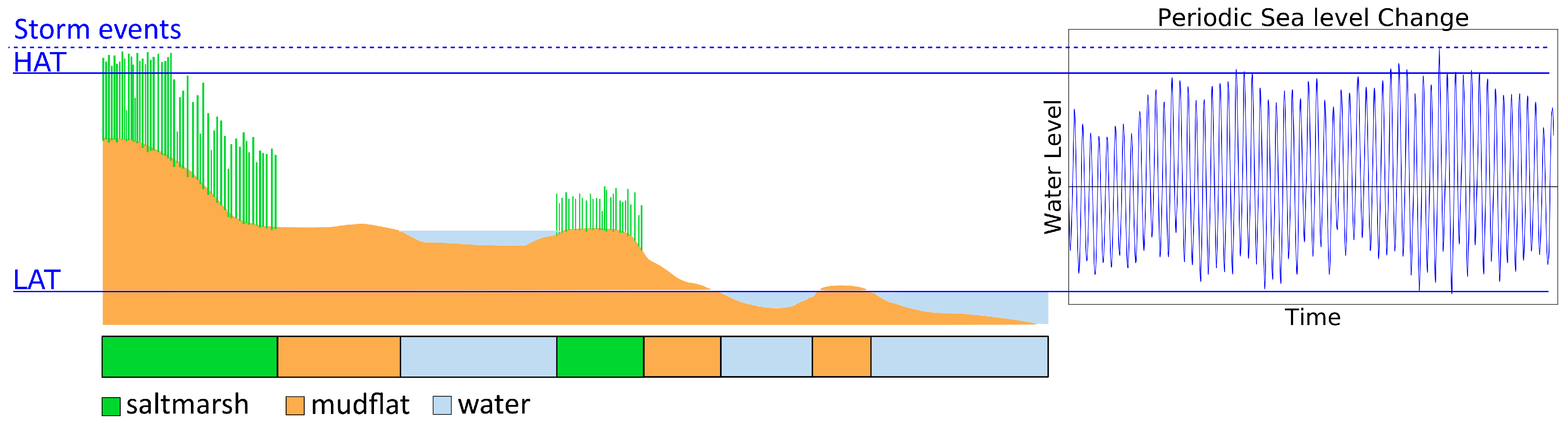
Coastal saltmarshes are located in intertidal zones and are periodically flooded due to astronomical tides and storm events [1]. With our method, we classify saltmarsh, mudflat, and open water. We define saltmarsh as the vegetated intertidal area and mudflat as the unvegetated intertidal area in this coastal ecosystem. As illustrated in Figure 1, periodic sea level changes cause the vegetated marshes as well as the unvegetated mudflats (s.l., these can also be, e.g., sandflats) are regularly or intermittently covered with water and are therefore not always visible from space. Open water is defined where area is covered with water at any tidal situation. The amplitude and frequency of the periodic sea level changes vary between sites [36].

Consequently, for the classification of this intertidal area based on one satellite image, we would need this image to show a lowest astronomical tide situation. This means that we need local tidal information to find such an image, if it even exists. In order to classify an image without the need for tidal information, we perform unsupervised classification on several images in an image collection containing images at different tidal situations over a specific period of time. A classified image resulting from such an image collection is hereafter referred to as time step. In theory, if we detect saltmarsh in one of the images within an image collection of one time step, we can conclude that this image is the one recording a tidal situation in which saltmarsh is exposed. For water, we can assume that a pixel which is water in all the images within the image collection of one time step is open water. However, in practice, satellite images, even if atmospherically corrected, are contaminated by e.g., atmospheric influences and radiometric noise and classification errors occur. Moreover, short-term variations occur due to actual changes of the classes in these ecosystems such as marsh and mudflat erosion and expansion [2,37,38,39] or seasonal changes of the vegetation. Therefore, our method requires a minimum fraction (hereafter referred to as frequency threshold) of the images in the image collection to be classified as saltmarsh or water, before it is classified as such for the given time step. Furthermore, we found that we need the given image collection to contain satellite images over three years to have sufficient observations for the classification decision, mainly due to high cloud cover in some areas. Consequently, a classified image for a given time step is based on data over three years in line with the long-term (interannual) changes we are focusing on in this paper. This procedure and the frequency threshold selection are described in detail in Section 2.4.

2.2. Data Description

Landsat data are commonly used for land cover classifications due to the feasibility of their spatial resolution (30 m), revisit period (16 days), spatial coverage (185 × 185 km), and their consistency over time [26,29]. We applied our method to Landsat data as these specifications are suitable for our approach as well.

We used surface reflectance data from the Landsat Surface Reflectance Climate Data Record (Landsat CDR) data set provided by the United States Geological Survey (USGS) and NASA and processed by the Landsat Ecosystem Disturbance Adaptive Processing System (LEDAPS). This Landsat Level-2A product includes atmospherically corrected Landsat 4-5 Thematic Mapper (TM), Landsat-7 Enhanced Thematic Mapper Plus (ETM+), and Landsat-8 Operational Land Imager(OLI) images at a global scale, covering the time period from 1982 to 2018. Results from assessments of the Landsat CDR surface reflectance data showed that the images are suitable as ready-to-use products for environmental studies, especially over large areas [40,41].

We developed and implemented our classification procedure in Google Earth Engine (GEE) and obtained the Landsat products from the GEE data catalog. GEE is a browser-based developer platform for geospatial and remote sensing analysis with access to a multi-petabyte database of satellite images and products.

We only included Landsat 5 TM imagery in this study, which covers the time period from 1985 to 2011 (27 years) because systematic biases appear among the sensors, which would lead to inaccurate and inconsistent time series, and affect products like the normalized difference vegetation index (NDVI) [42].

We focus on coastal waters and intertidal areas. Therefore, we masked all other areas based on the CORINE Land Cover 2012 (CLC2012) inventory (see Section 2.4) provided by the European Environment Agency (EEA). This product has been derived from satellite data and provides land cover information for the whole of Europe containing 44 different land cover classes and has a spatial resolution of 100 m [43].

2.3. Detecting and Masking Unusable Data

We performed saltmarsh classifications for European saltmarshes based on surface reflectance Landsat 5 TM data covering the time period 1985 to 2011. The Landsat 5 TM surface reflectance images come with image properties providing image quality assessment and percentage cloud cover. Before we perform the decision tree classification chain illustrated in Figure 2, we use these properties to filter for images with a quality assessment greater than 7 (0 = worst, 9 = best) and cloud cover lower than 60%. Within a filtered image collection, we used the provided pixel quality assessment (pixel_qa) band to mask clouds, cloud shadows, as well as snow and ice. Furthermore, we use the atmospheric opacity (sr_atmos_opacity) band to mask pixels characterized by high atmospheric contamination and the radiometric saturation (radsat_qa) band to mask oversaturated pixels.

A classified image of a given time step represents an image collection of three years as we are interested in long-term habitat changes and our method requires sufficient observations for each pixel, which is not given by smaller image collections due to atmospheric influence from clouds, cloud shadow, or aerosols and erroneous pixels. With a given time step resulting from an image collection over three years, we also avoid confusing short-term variability of reflectance values with actual habitat variability [22,30]. Furthermore, sufficient images recorded during different water levels are needed, in order to discriminate between intertidal areas and permanent water (see Section 2.4).

After masking unusable pixels, we analyze data availability. We calculate data availability per pixel, i.e., the count of how often a pixel is not masked from all the images in the three years’ image collection of each time step. Then, we calculate the mean value of this per-pixel data availability over the area the method is applied to and exclude a whole time step from the classification if this mean value is below 10 images. With this, we already exclude time steps based on image collections containing a high amount of cloudy satellite images, thus preventing large areas of the study sites from being masked. This would happen because we then look at the per-pixel number of available images and mask out those pixels in each time step with less than 5 observations because the smaller the number of observations, the more likely it is that no image at the lowest tide exists in an image collection. We found these thresholds empirically by looking at the classification results of different study sites with different thresholds and compared those to high resolution images in Google Earth. To allow for a comparison over time, the same pixels have to be masked in all time steps of the generated time series. Therefore, a mask is applied in the end of the procedure, to mask all the pixels which have been masked in any time step over the time series in a specific study area.

2.4. Unsupervised Saltmarsh Classification Procedure

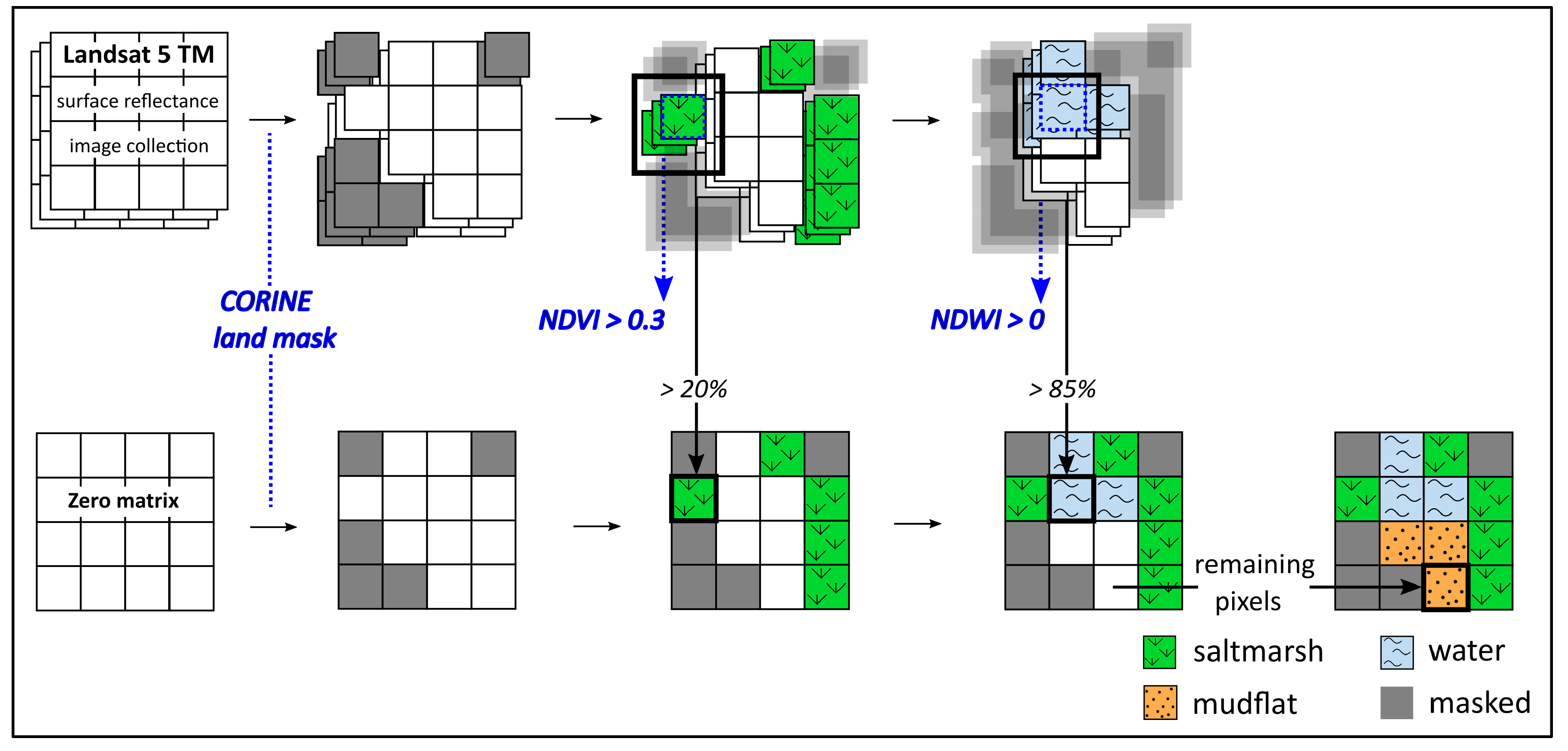
The classification procedure follows an univariate decision tree (DT) classification approach [34,35] by making step by step decisions for each pixel (Figure 2). It is a simple, flexible approach which allows for integrating other environmental data and can be applied on different scales [25,26,34,35].

We start the classification procedure by masking land areas using additional land cover information. This is necessary to exclude terrestrial vegetation, which would be detected as saltmarsh area in our method. In order to do that, we build a land mask by reclassifying the CORINE CLC2012 data set. This land mask included all CORINE land cover classes except maritime wetlands (saltmarshes, intertidal flats, salines) and marine waters (coastal lagoons, estuaries, ocean). Together, these maritime wetland and marine water classes, which are all non-terrestrial data, define the area of interest for our further classification. For the pixels within this non-terrestrial area, which meet the requirement R_RED > 0% and R_NIR > 2% [32], we calculate the Normalized Difference Vegetation Index (NDVI) [44,45]

$$\mathrm{NDVI}=\frac{{\mathrm{R}}_{\mathrm{NIR}}-{\mathrm{R}}_{\mathrm{RED}}}{{\mathrm{R}}_{\mathrm{NIR}}+{\mathrm{R}}_{\mathrm{RED}}},$$

(1)

where vegetation is defined as NDVI >0.3. We chose this threshold to be >0.3 to not include algae that may occur on the mudflats [32]. The classification is done for each of the satellite images. We then classify a pixel as saltmarsh in the three-year result if it is classified as vegetation in more than 20% of all the classified images in a specific three year image collection for that pixel. By setting a threshold, we avoid overestimation of saltmarsh area due to, for example, erroneous pixels, or blooms of benthic algae. After that decision, we move to the next decision step for the remaining pixels. We calculated the Normalized Difference Water Index (NDWI) [46]

$$\mathrm{NDWI}=\frac{{\mathrm{R}}_{\mathrm{GREEN}}-{\mathrm{R}}_{\mathrm{NIR}}}{{\mathrm{R}}_{\mathrm{GREEN}}+{\mathrm{R}}_{\mathrm{NIR}}},$$

(2)

where water is defined as NDWI > 0. Again, this is done for all the images. We classify a pixel finally as water if it is classified as water in more than 85% of all classified images in the image collection of the respective three-year time step for a specific pixel. We chose this frequency threshold (Section 2.1) to take into account the fact that water may not be detected in all the images with the chosen NDWI threshold. Considering the fact that, for some pixels, only a small amount of observations are available, a higher frequency threshold would result in underestimation of water pixels if misclassification occurs in only a small amount of images within the image collection. At the same time, the frequency threshold cannot be too low as it would overestimate water and underestimate mudflats considering the possibility of very high water levels which occur less often (e.g., spring tide, storms). After having classified first the saltmarsh pixels, and then the water pixels, the remaining pixels are intertidal, not-vegetated areas, here classified as mudflat.

The order of decisions starts with the classes that are most distinguishable from other land cover classes with optical satellite data, followed by those that are more likely to be confused with other land cover classes. Specifically, we chose to classify vegetated areas before detecting water pixels as dark vegetated areas can result in high water index values, which would lead to false detection of water [31], and with this an underestimation of saltmarsh habitat.

2.5. Thematic Classification Performance

To validate the classification, we obtained data of the Western Scheldt from Rijkswaterstaat, the Dutch Ministry of Transport, Public Works and Water Management. They provide spatial data that give information on emersion frequencies and define a threshold (of 4% emersion time) below which the area is defined as water. We used this data set to validate the distinction between water and mudflats in our classification by reclassifying this according to Rijkswaterstaat’s definition of a pixel being water with a flooding frequency >96%. The data set is based on echo sounding and laser altimetry bathymetric data, coupled to a hydrodynamic model SCALWEST [47,48]. In addition, we used their geomorphological maps of the Western Scheldt, based on 1:10,000 false color aerial photographs [49]. From this data set, we extracted the area that is defined as saltmarsh with >50% vegetation cover, to validate our saltmarsh detection.

From these data, we extracted the classes saltmarsh, mudflat and water. Subsequently, we compare each pixel in our classification result to the respective pixel in the validation data set. Both data sets were masked to the CORINE data set as described above, in order to consider misclassifications arising from the use of CORINE classification as land mask. Furthermore, we masked those pixels in the validation data set, which are masked in the classification result due to missing data. We validated the results of the saltmarsh-mudflat–water classification of the Western Scheldt for the time steps 1995 (with a validation data set from 1996), 2004, 2007 (emersion frequency data set from 2008) and 2010 as validation data that are available for these years. We performed the validation in Google Earth Engine (GEE-script https://code.earthengine.google.com/81b0eca8b4c14d3083660ac3c06c2e46).

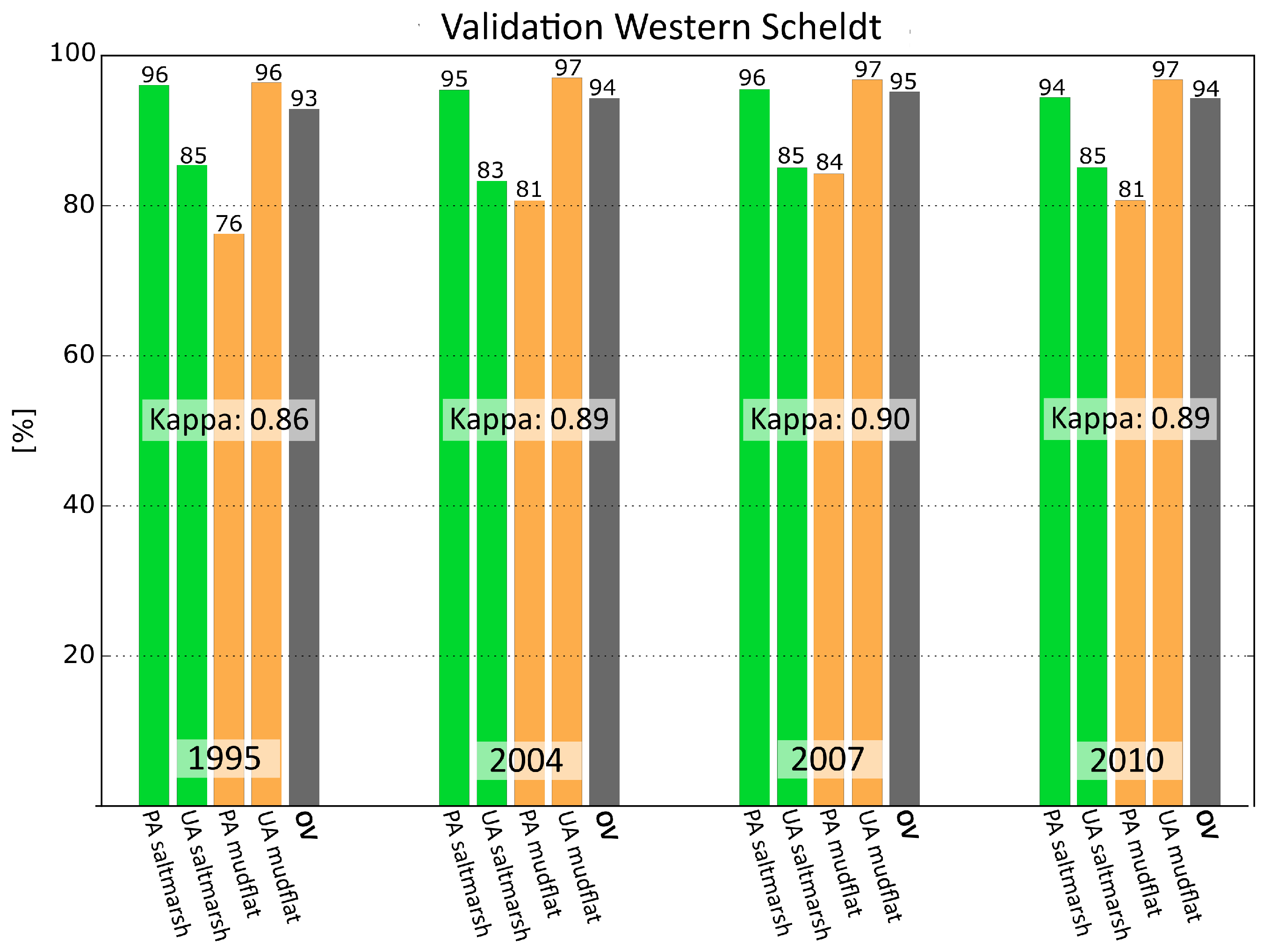
We computed user accuracy (UA) and producer accuracy (PA), as well as overall accuracy (OA), and the Kappa coefficient as described in Stehman (1997) [50]. The OA is the ratio of correctly classified pixels and the total number of pixels in the image. The UA for class x is the probability that a pixel defined as class x in the classification result is defined as class x in the validation data set as well. The PA for class x is the probability that a pixel defined as class x in the validation data set is defined as class x in the classification result as well. The Kappa coefficient is another variable to assess the overall classification performance. It can be a value between −1 and 1, with 1 indicating a full concordance [50].

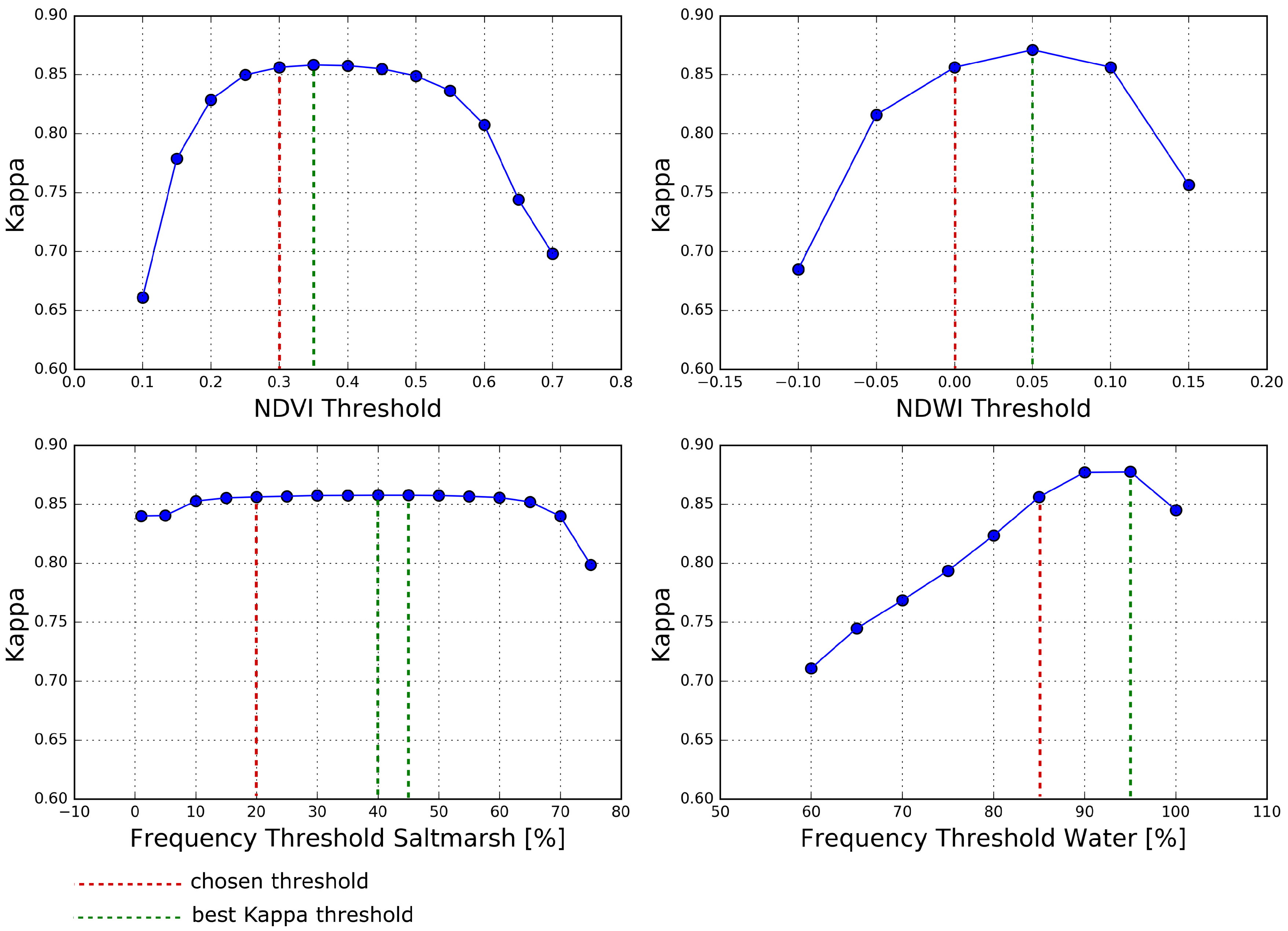
We additionally performed sensitivity analysis using the validation data set of the Western Scheldt of 1996. We tested the sensitivity of the method to the chosen NDVI and NDWI thresholds as well as to the chosen frequency thresholds of the image collections. We did this by performing our classification procedure with different thresholds and computing the Kappa coefficient as described above.

2.6. Method Implementation Using Other Sensors

For further assessment of our classification method, we performed the unsupervised saltmarsh classification based on Landsat 7 ETM+ data and correlated predicted saltmarsh area and predicted mudflat area based on Landsat 5 TM data to those based on Landsat 7 ETM+ data, for the time steps of the overlapping time period of both sensors (2001–2010). We included as many of our study sites as possible, but excluded those sites for which less than two overlapping time steps in the time series were available due to high cloud cover or low quality images. Time steps of the Landsat 7 ETM+ time series were excluded under the same conditions as done in the Landsat 5 TM time series (see Section 2.3). With this trend comparison, we assessed the consistence of the unsupervised DT classification approach and checked whether or not it is applicable for saltmarsh classification using data from other sensors than Landsat 5 TM.

2.7. Method Application

We applied our method to look at saltmarsh changes across Europe. We included the European saltmarsh sites until 58${}^{\circ }$ North, which are documented by McOwen et al. (2017) [4]. From this global data set, we included all European saltmarsh sites (systems with saltmarsh and mudflat and/or water) larger than 20 km², as well as 16 sites between 5 km² and 20 km², provided the resulting time series had at least six time steps, as for some regions high cloud cover led to many missing data points in the time series. Furthermore, we aimed to select whole basins, bays, or estuaries comprising several saltmarshes.

Under these requirements, we included 125 study sites covering the North-Atlantic/North Sea, the Baltic Sea, and the Mediterranean Sea. We applied our unsupervised classification procedure to these study sites in Google Earth Engine (GEE).

In order to detect saltmarsh habitat change, we performed trend analysis of the resulting time series derived for each study site. As the study sites vary in size, we performed this for both absolute (km²) and relative (%) saltmarsh area. Due to strong atmospheric influences in some areas and erroneous pixels caused by the sensor’s technical limitations, data availability is reduced in some areas, which partly resulted in missing pixels and outlier values. Therefore, we chose the Mann–Kendall trend test [51,52] to test for a significant linear upward or downward trend with a significance level of 0.05. This non-parametric test does not require normally distributed data and is robust against missing and outlier values, which makes it suitable for trend detection in the derived time series.

We additionally compared the trends of the different seas by calculating the mean area of saltmarsh and mudflat (km²) over the investigated time period 1886 to 2010 for the North Atlantic/North Sea basin, the Mediterranean Sea, and the Baltic Sea. Then, we applied the Mann–Kendall trend test to the resulting time series, as done for the study site’s time series of the saltmarsh area.

We performed the statistical data analysis in the programming language Python. The results were visualized in QGIS 3.0.

2.8. Alternative Global Application

We tested a solution to apply our method on a global scale. We produced a global land mask aiming to mask land areas without masking saltmarsh area which is often classified as land class in land cover data sets. We used the global land cover data set GlobCover 2009 derived from ENVISAT’s Medium Resolution Imaging Spectrometer (MERIS) provided by the European Space Agency (ESA) at 300 m spatial resolution and combined this with the saltmarsh polygons by McOwen et al. (2017). We converted the saltmarsh polygons by McOwen et al. (2017) to raster data and uploaded the resulting data set to GEE. Then, we masked all the pixels which are neither water according to GlobCover 2009 nor defined as saltmarsh area by any McOwen polygon.

We used this mask and applied our method to the same 125 study sites across Europe, and calculated the relative trends (%/year) and the absolute trends (km²/year) for each study site, in the exact way as done using CORINE data to mask land. We compared the trends resulting from the DT classification procedure using CORINE data as land mask (hereafter referred to as European land mask solution) and the trends resulting from the DT classification procedure using a combination of GlobCover 2009 and saltmarsh polygons by McOwen et al. (2017) (hereafter referred to as global land mask solution).

3. Results

3.1. Unsupervised Saltmarsh Classification Procedure

The work results in an GEE-script where the Western Scheldt functions as a template for the application to other areas (Appendix A). Users can change the definition of the desired location (latitude, longitude) and the definition of a region of interest polygon defining the study site. For sites outside Europe, we propose an alternative to the CORINE land cover data set as a solution to mask land areas, which is described in Section 2.8. Paragraphs can be commented out in the script to reduce the time series.

Depending on what is needed, the following exports are possible: (1) number of saltmarsh pixels for each time step, (2) number of mudflat pixels for each time step, (3) number of total pixels in each study area and (4) classified image for each time step.

3.2. Thematic Classification Performance

Figure 3 illustrates the results of the unsupervised saltmarsh classification’s validation, which we carried out for the Western Scheldt 199F5, 2004, 2007, and 2010. Both the overall accuracy exceeding 90% in all validated years and the Kappa coefficient always being above 0.85 indicate an almost perfect classification performance [53,54]. By comparing the saltmarsh’s PA and the saltmarsh’s UA, it can be observed that saltmarsh area is slightly overestimated as the UA for this class is always smaller than its PA. For mudflat pixels, the opposite can be observed.

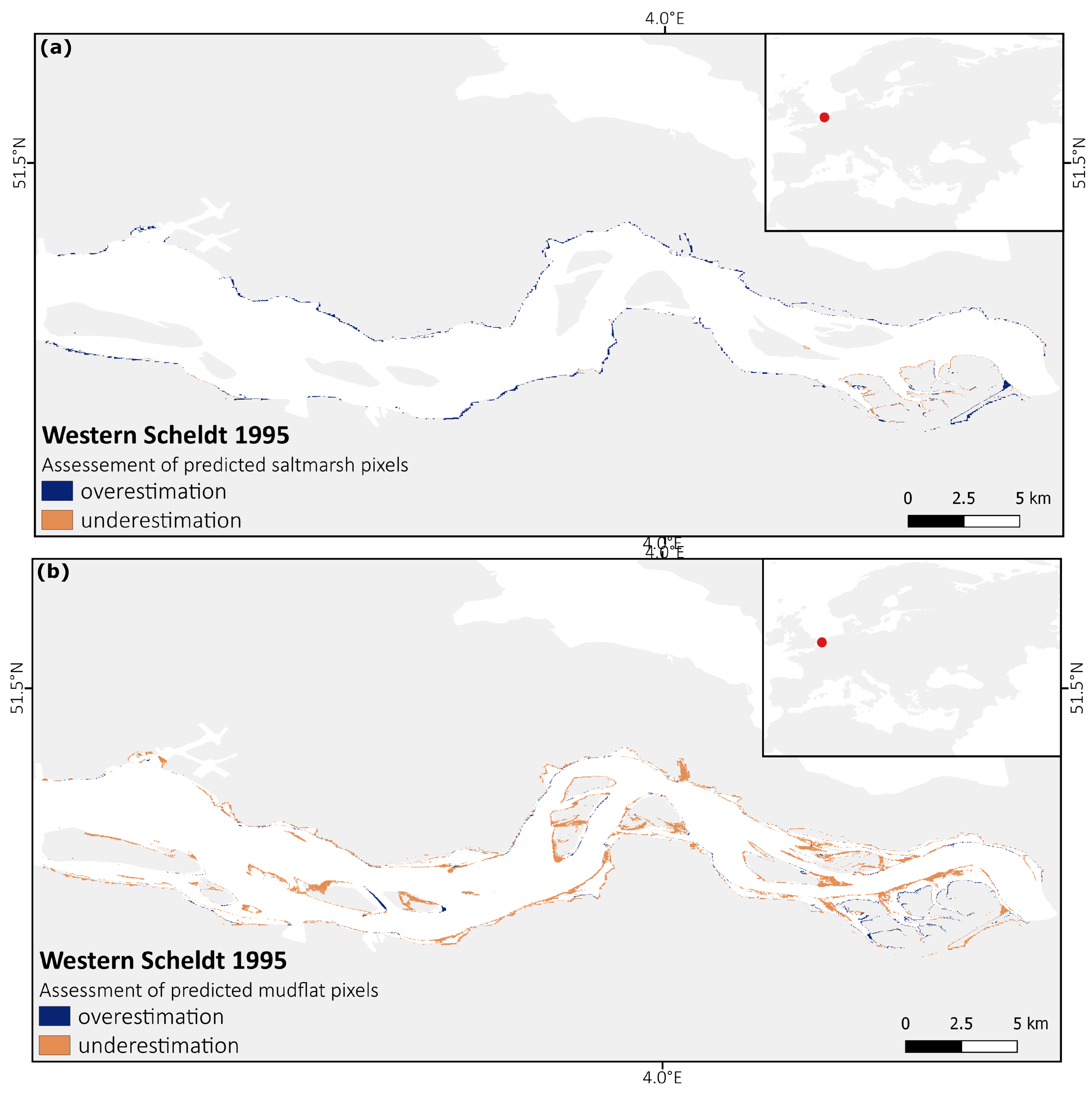
A change detection between the validation image and the classification result for the Western Scheldt in 1995 (Figure A1) gives a spatial overview about where misclassified pixels occur. Figure A1a shows where saltmarsh pixels have been wrongly classified as well as where saltmarsh area is overestimated (false positive) or underestimated (false negative). Figure A1b shows the same for mudflat pixels.

Misclassified saltmarsh pixels (Figure A1) mainly occur at the edge between land and coastal areas. Underestimation of saltmarsh can particularly be observed at the edges between the classes saltmarsh and mudflat. The overall amount of misclassified saltmarsh pixels is very low, which is shown by both, the results of the Kappa statistics (Figure 3), and the change detection between the validation image and the classified image of the Western Scheldt 1995 (Figure A1a). Compared to that, for mudflat pixels the results of the Kappa statistics (Figure 3) and the spatial overview (Figure A1b) show that misclassified pixels (mainly underestimation) occur primarily at the interface between mudflat and water.

The analysis of the method’s sensitivity to NDVI and NDWI thresholds as well as to frequency thresholds (Figure 4) indicates good classification performance in the Western Scheldt 1995 for a wide range of thresholds around the chosen ones. NDVI thresholds between 0.2 and 0.6 and NDWI thresholds between −0.05 and 0.1 result in Kappas above 0.8. Frequency thresholds which decide whether or not a pixel is saltmarsh in the final classification can range between 1% and 70% without the Kappa falling below 0.8. The frequency threshold for the decision about a pixel finally being water or not can range between 80% and 100% and still show good concordance between the classified image and the validation data set.

3.3. Method Implementation Using Other Sensors

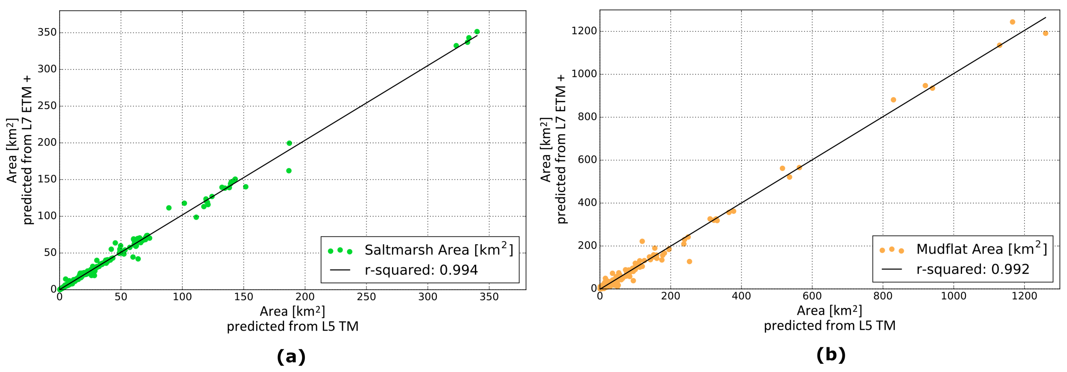
High correlations can be observed when comparing classification results predicted with Landsat 5 TM data and those predicted with Landsat 7 ETM+ data (Figure 5), for both saltmarsh (r-squared = 0.994, p = 0) and mudflat (r-squared = 0.992, p = 0). The slopes of the linear fit are 1.017 for predicted saltmarsh area and 1.005 for predicted mudflat area. Consequently, the area predicted from Landsat 5 TM and Landsat 7 ETM+ images is almost similar with slightly more saltmarsh area being classified from Landsat 7 ETM+ images than from Landsat 5 TM images.

3.4. Saltmarsh Change across Europe

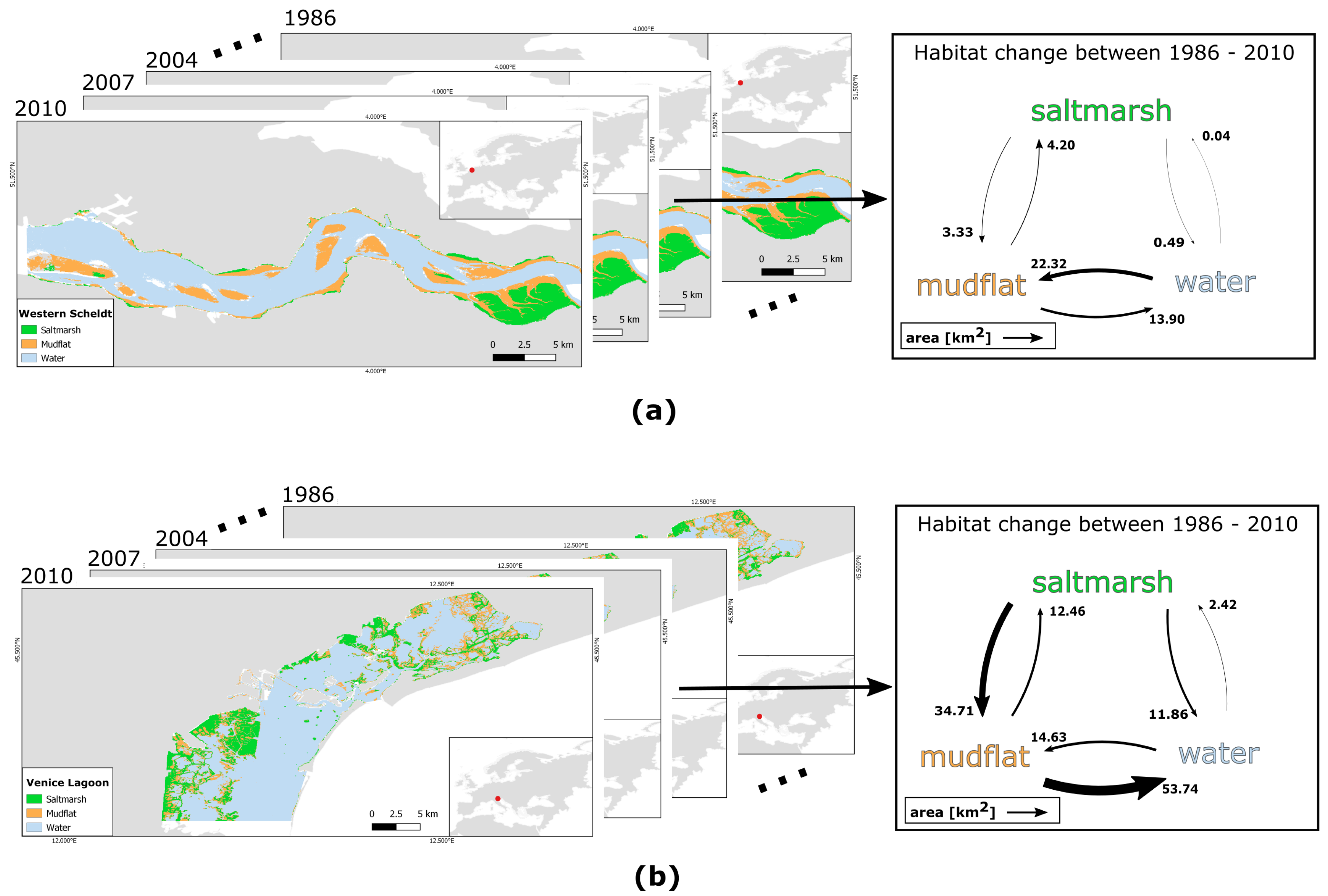
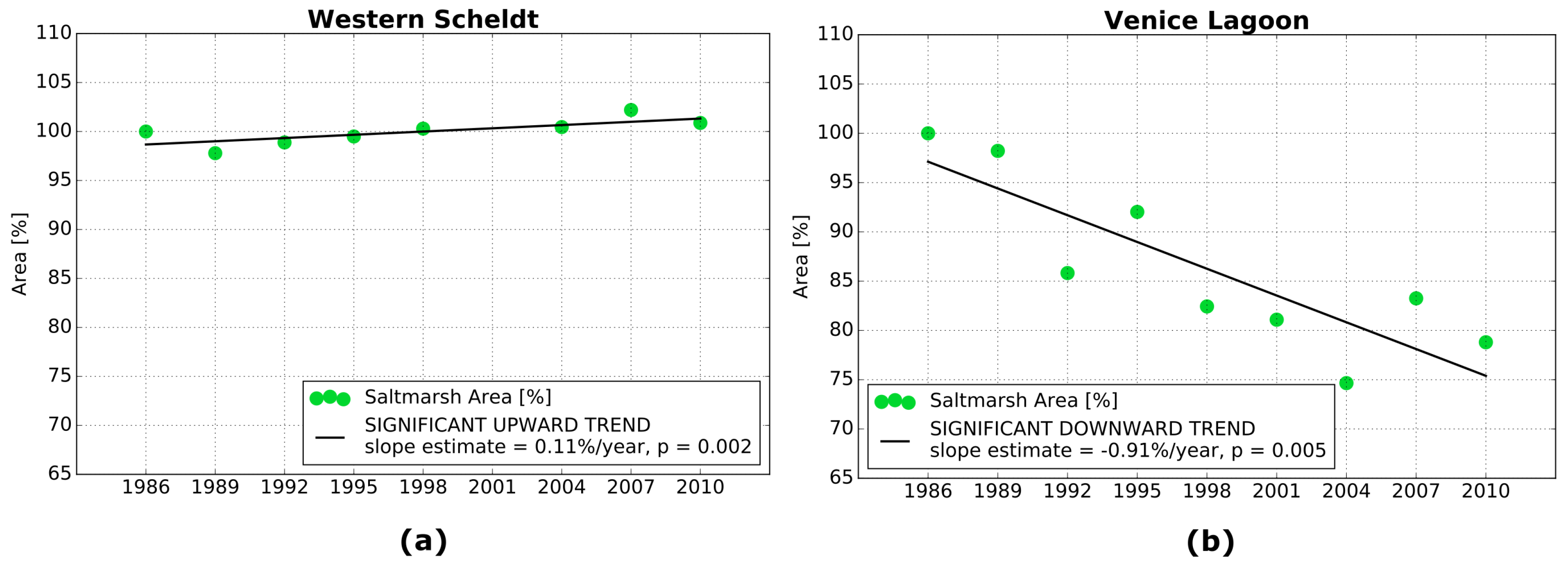
Resulting long-term changes in saltmarsh area of the 125 study sites are provided as an Excel-sheet in the supplementary material. Figure 6 shows time series of the classification results for the Western Scheldt and the Venice Lagoon. These study sites are shown here as examples with the Western Scheldt experiencing overall saltmarsh gain and the Venice Lagoon experiencing overall saltmarsh loss relative to mudflat and open water. Missing values can be observed, resulting from unusable pixels like clouds, cloud shadows, snow, or low quality pixels being masked during the decision tree classification procedure. This especially occurs in areas with high cloud cover, like the Western Scheldt.

The ability to derive saltmarsh classification time series from 1986 to 2010 for each study site, allows for observing the dynamics in the intertidal zone. This is illustrated in Figure 6 in the right part for the examples Western Scheldt and the Venice Lagoon. It shows the area size of each class becoming another class when comparing time step 1986 and time step 2010. In this example, in the Western Scheldt, net transition was largest from class water to mudflat, whereas, in the Venice Lagoon, net transition was largest from mudflat to water, followed by a net transition from saltmarsh to mudflat.

Figure 7 shows the relative trends in saltmarsh area for the two examples, the Western Scheldt and the Venice Lagoon. For the Western Scheldt, a significant upward trend of saltmarsh area can be observed from 1986 (47.817 km²) to 2010 (48.236 km²), whereas, in the Venice Lagoon, the saltmarsh area is decreasing significantly over time (from 149.345 km² in 1986 to 117.661 km² in 2010).

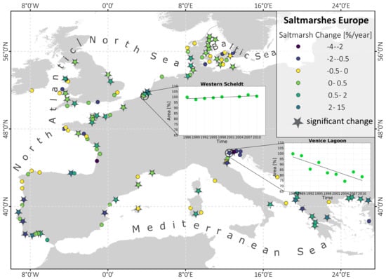
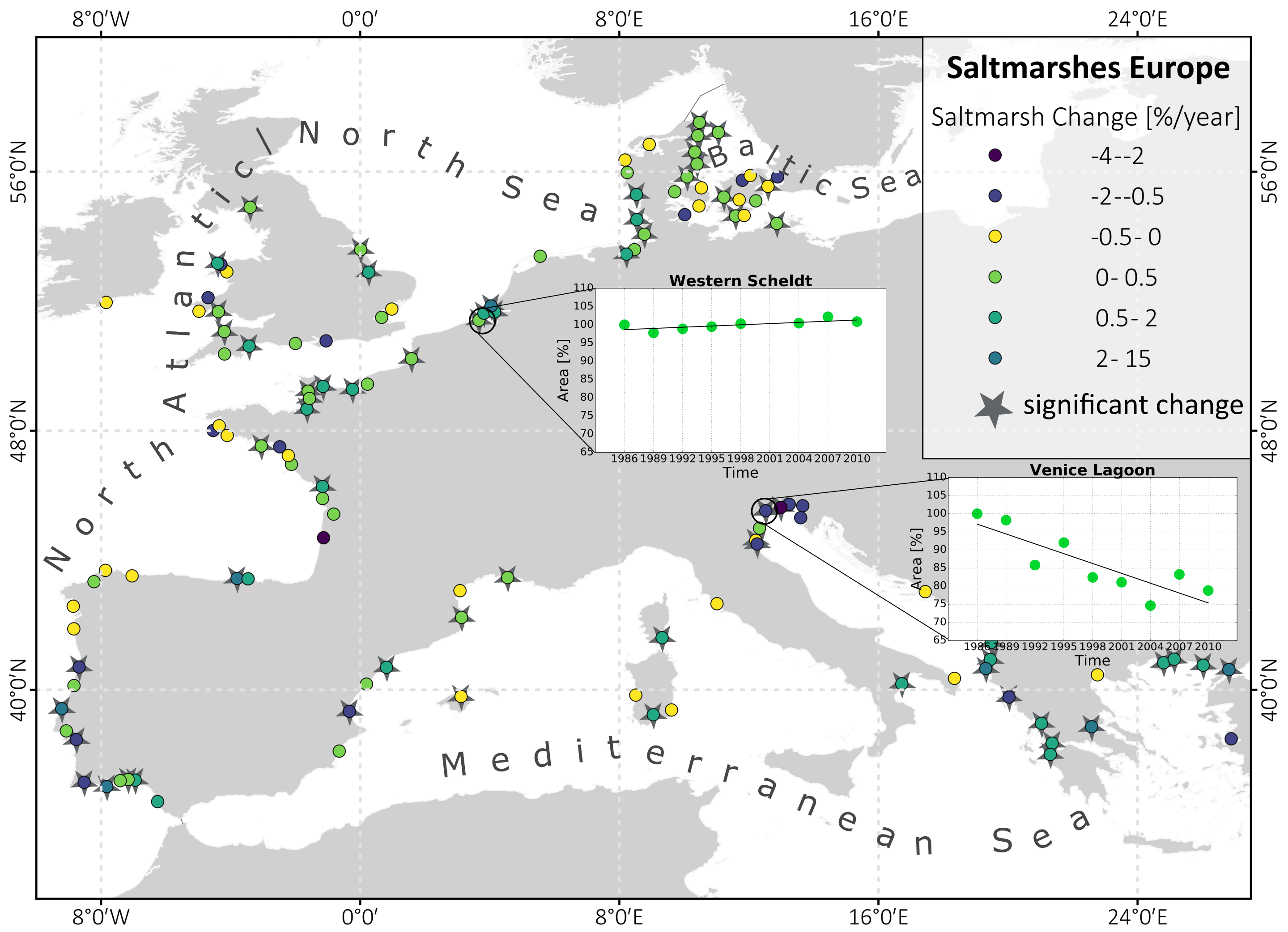
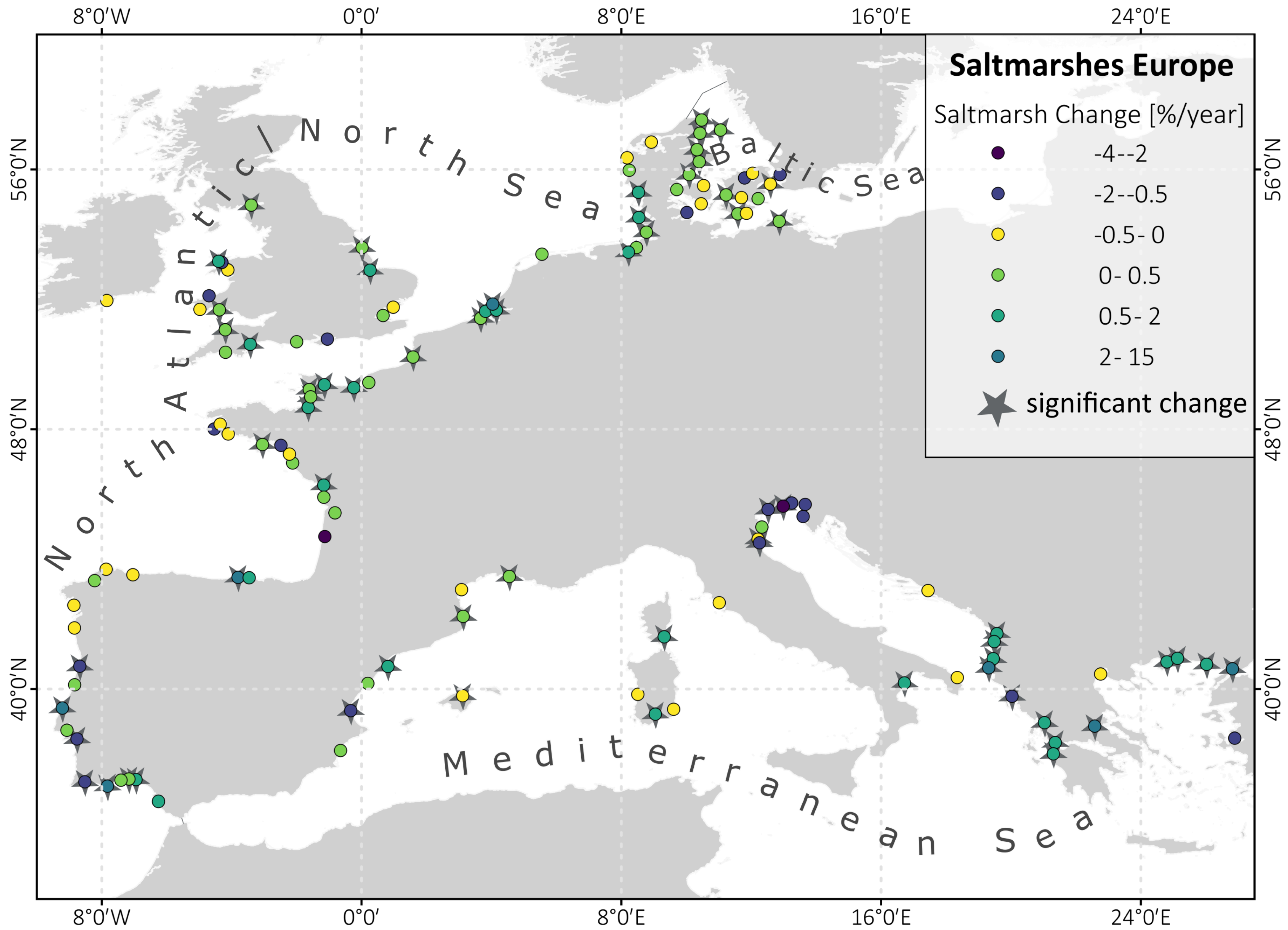
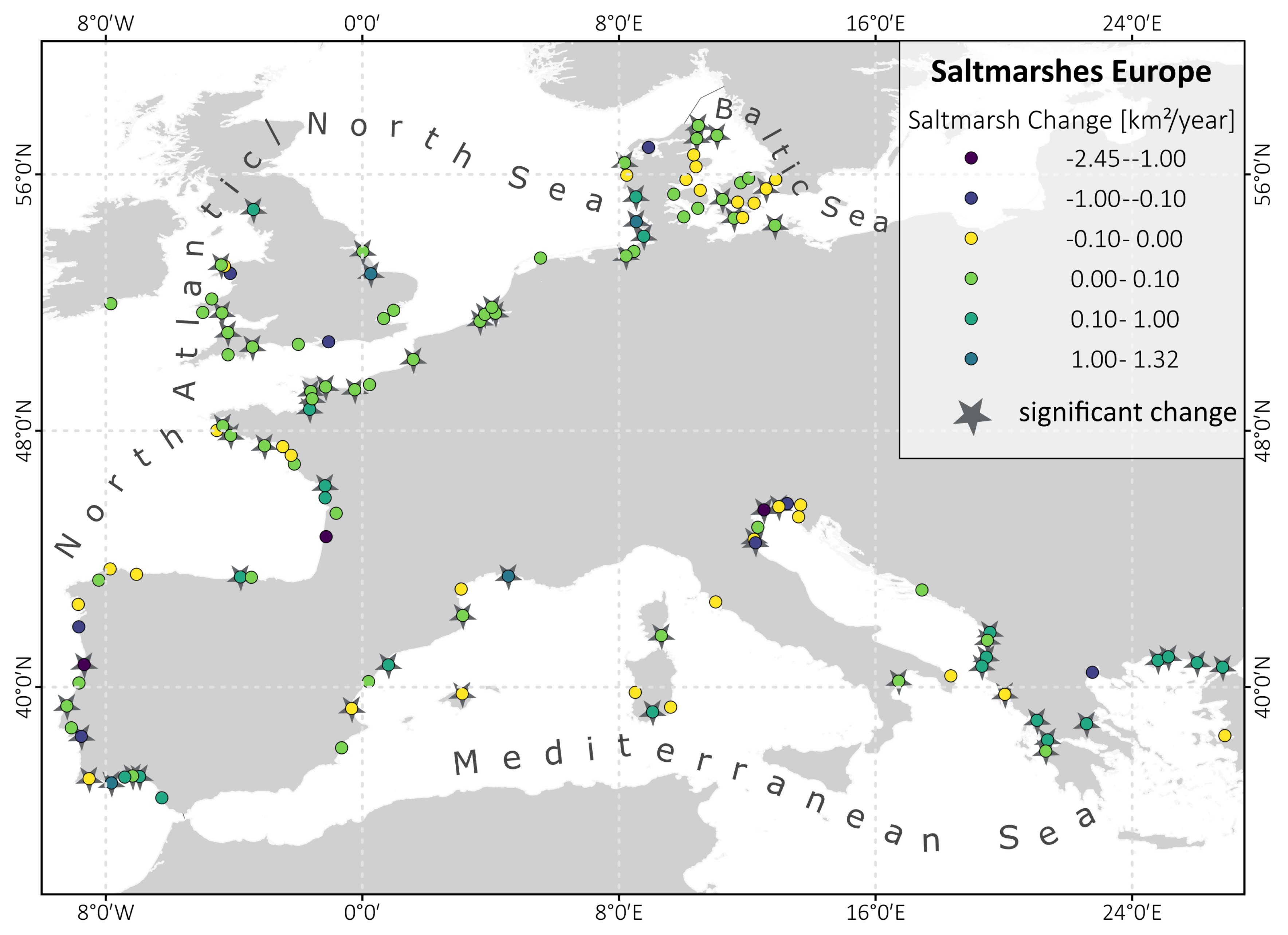
Based on such time series analysis for 125 study sites, we generated maps showing trends of seaward saltmarsh change across Europe. Annual rates of relative seaward habitat change (%) from 1986 to 2010 are illustrated in Figure 8, whereas annual rates of absolute habitat change (km²) of the same locations are provided in Figure A2. The stars indicate that a significant upward or downward trend was detected by the Mann–Kendall trend test. A third map shows how the selected study sites vary in size (Figure A3).

Trends of saltmarsh extent at the seaward boundary from 1986 to 2010 vary in space and some patterns can be observed by comparing the detected rates of relative habitat change of the three seas: the majority of the study sites in the North Atlantic/North Sea basin experience significant gain in saltmarsh area, especially in the northern part. The highest rates of relative saltmarsh gain (2 to 15%) can be observed along the Dutch coast, the coast of Northern Spain, and at the Portuguese coast. Sites with lower, but significant relative rates between 0.5% and 2.0% appear along the North Atlantic coast, as well as rates <0.5%. High rates of saltmarsh loss can also be observed in the North Atlantic/North Sea along the Portuguese coast. In the Mediterranean Sea, saltmarshes at the Albanian and the Greece coast show predominantly saltmarsh gain with yearly rates of 2 to 15% and rates of 0.5 to 2%, whereas, on the north-east coast of Italy, the Slovenian, and the Croatian coast high rates of saltmarsh loss may occur (−4% to −2% and −2% to −0.5%). Furthermore, several study sites show very small rates (<0.5%), often detected as not significant trends. In the Baltic Sea, most of the sites show significant saltmarsh gain, but at very small rates (<0.5%).

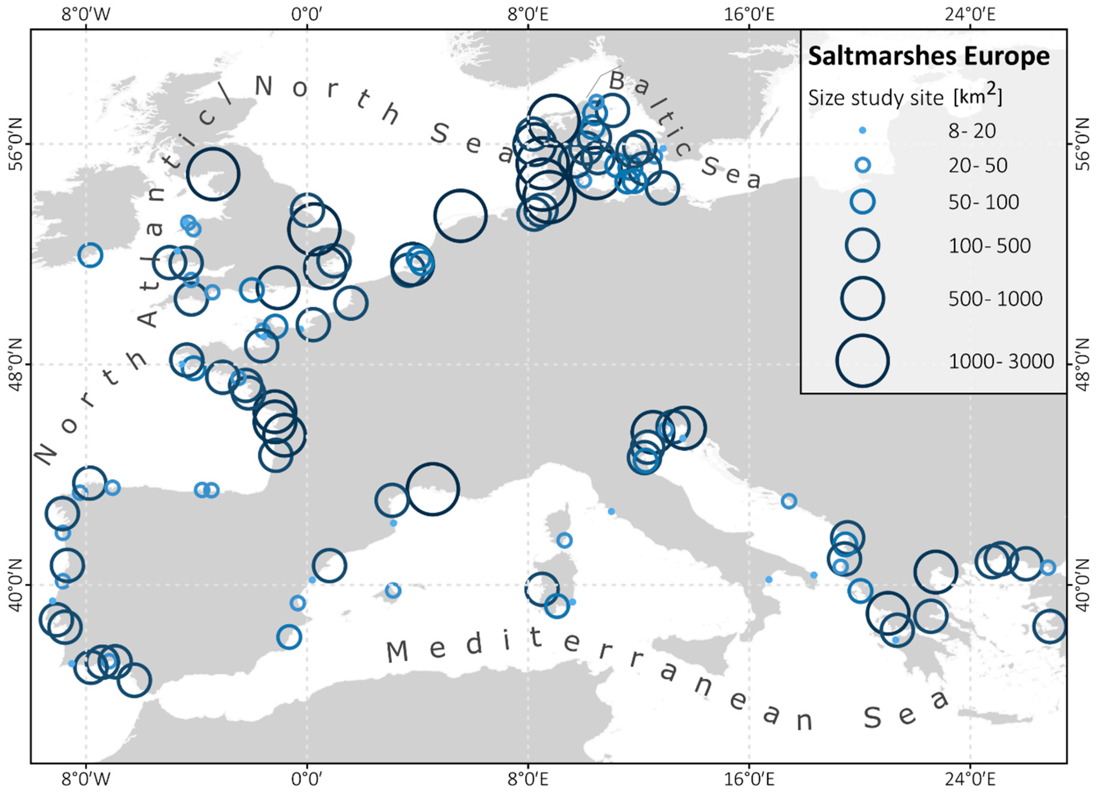
The smallest study site covers an area of about 20 km² and the largest study site covers an area of about 8330 km², which makes it important to look at both absolute and relative saltmarsh dynamics. Nevertheless, both maps show similar patterns (Figure 8 and Figure A2).

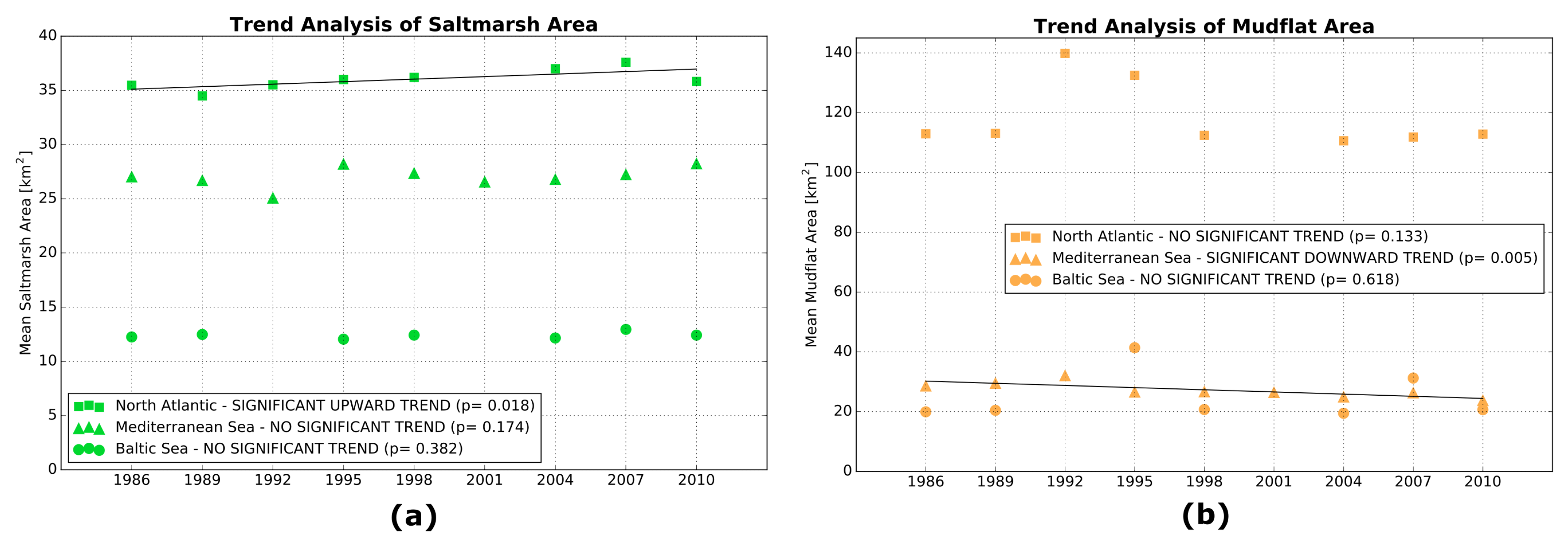
Figure 9 shows a time series of mean saltmarsh area and mean mudflat area of all study sites in the North Atlantic/North Sea basin, the Mediterranean Sea, and the Baltic Sea.

Mean saltmarsh area differs between the European seas with the largest in the North Atlantic/North Sea ranging from 33.2 km² to 36.6 km². Mean saltmarsh area in the Mediterranean Sea ranges between 26.3 km² and 29.6 km², and the smallest mean saltmarsh area can be observed in the Baltic Sea (12.1 km² to 12.6km²). The same order applies for mean mudflat area which is by far largest in the North Atlantic/North Sea, albeit the mean mudflat area size in the Mediterranean Sea is almost the same as in the Baltic Sea.

Mean saltmarsh area is increasing significantly in the North Atlantic/North Sea with a yearly rate of 0.09 km² per year. For the mudflat area in the Mediterranean Sea, a significant downward trend has been detected with −0.23 km² per year.

3.5. Alternative Global Application

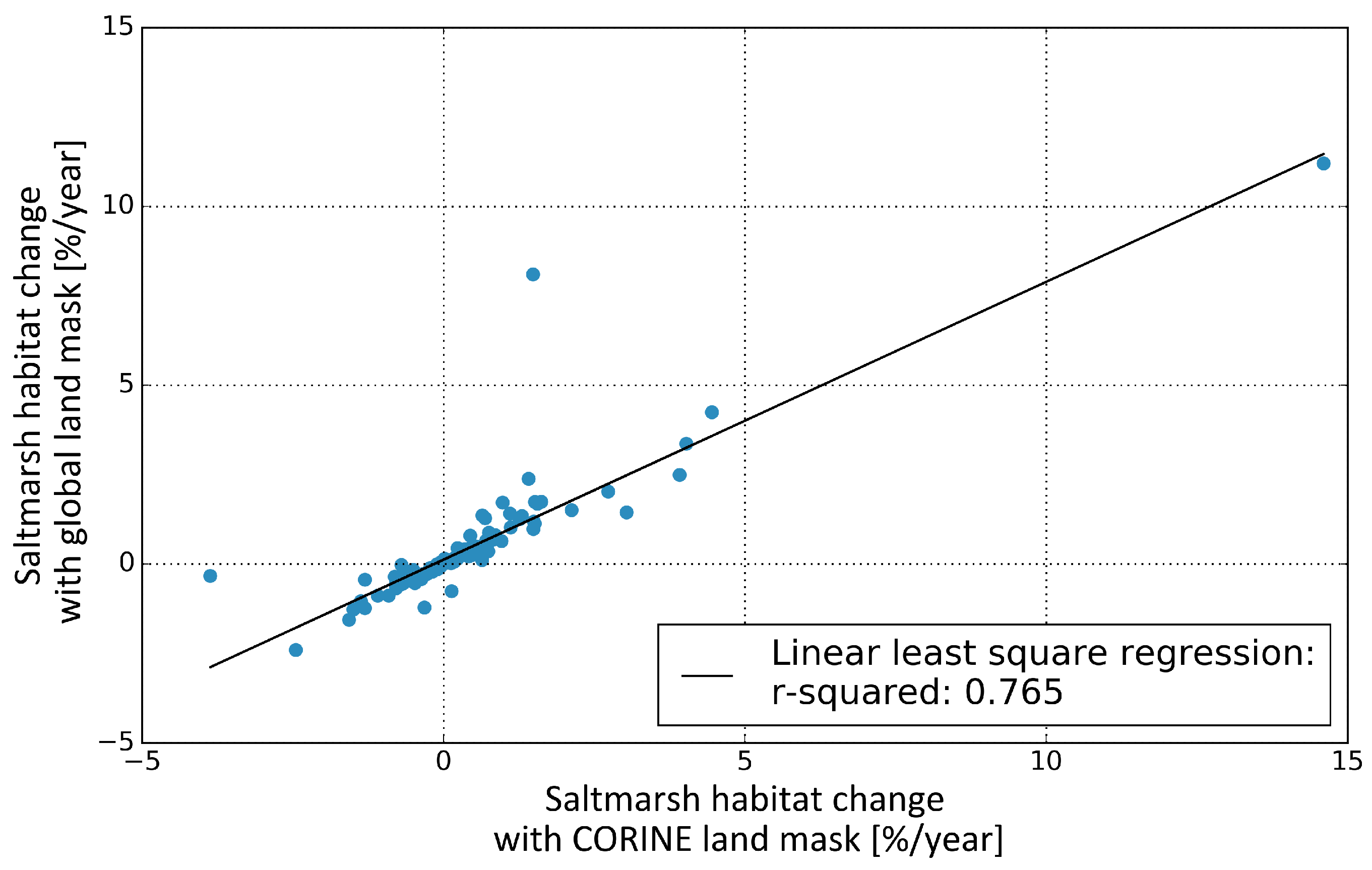
Figure 10 shows the correlation between the relative trends (%/year) resulting from the European land mask solution and the trends resulting from the global land mask solution.

The plot shows a high correlation (r-squared = 0.765, p = 0). Two outliers can be observed; the study sites Kotychi Lagoon (ID 35 in Table S1, Supplementary Material) with a significant trend of 1.49%/year (European land mask solution) and 8.10%/year (global land mask solution); and the study site Bibione Lagoon (ID 48) with a significant trend of −3.87%/year (European land mask solution) and a non-significant trend of −0.34%/year (global land mask solution). For four study sites, the trend’s sign changes with the method from negative (European land mask solution) to positive (global land mask solution), but none of these trends are significant. The slope of the linear fit (0.777) shows overall stronger yearly changes in saltmarsh area predicted by the European land mask solution than predicted by the global land mask solution.

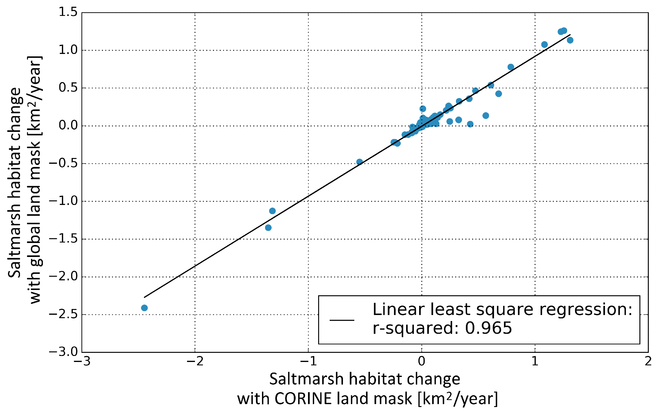
The plot comparing the absolute trends (km²/year) resulting from the European and the global land mask solution (Figure A4) shows an even higher correlation between the estimated trends (r-squared = 0.965, p = 0). The slope of the linear fit (0.926) being very close to one demonstrates that the absolute yearly trends are very similar for the two methods.

4. Discussion

4.1. Unsupervised Saltmarsh Classification Procedure

This method can easily be applied to multiple saltmarsh sites worldwide, enabling investigations on different scales, without the need for training areas. Furthermore, the user does not have to search for single images of particular sites, in order to find cloud-free images and deal with changing tidal water levels. Instead, these issues are solved in the classification procedure by using multi-temporal image collections.

4.2. Thematic Classification Performance

The presented method to classify saltmarshes unsupervised achieved an almost perfect performance [53,54] for the Western Scheldt at all available data sets. The classification of saltmarsh area was more successful than the classification of mudflat area. This is shown by the results of the Kappa statistics, the spatial overview of misclassified pixels, as well as the plots of predicted saltmarsh area and predicted mudflat area derived from Landsat 5 TM and Landsat 7 ETM+ data.

The observation that most of the overestimated saltmarsh pixels occur at the edges between saltmarsh and land areas can be explained by technical limitations: We used the CORINE land cover data set to mask land areas. Its low spatial resolution of 100 m led to overestimation of saltmarsh area because the 100 m × 100 m pixels covered parts of the vegetated land areas. Underestimation of saltmarsh pixels mostly appears at the edges between saltmarsh and mudflat because the geomorphological data defining saltmarsh area are provided as vector data sets. In order to use these data sets for validation, we had to convert them from vector to raster data, which produced mixed pixels at the edges of the vector data sets. We defined those mixed pixels as not being saltmarsh pixels in the validation image, accepting underestimation of saltmarsh area according to the validation. Despite misclassifications emerging from the described technical limitations, only very few wrongly classified saltmarsh pixels can be observed.

Overestimated mudflat pixels occur at the same positions where saltmarsh area was underestimated caused by the same technical limitations as described for saltmarsh pixels. Nevertheless, for predicted mudflat pixels, there is a greater mismatch between the validation image and the classified image, which cannot be explained only by technical limitations. Underestimation of mudflat pixels mainly occurs at the mudflat–water interface. It may result from the combination of three error sources: (1) We used validation data sets provided by Rijkswaterstaat showing flooding frequencies of a certain year. Our classification results for this year represents three years, thus actual changes may have occurred, especially regarding the dynamic interface of the intertidal and subtidal zones; (2) The detection of the exact edge between mudflat and water depends on the available number of observations for each area, as we conclude about intertidal and subtidal pixels based on their flooding frequencies. This approach implies misclassification if the tidal levels are above low tide in most of the available images for the respective area and time step. This results in underestimation of mudflat area, as these parts appear to be always covered with water. We presume that this may occur in other areas as well, especially in those with high cloud cover. (3) The order of decisions in the decision tree (DT) classification procedure may additionally lead to falsely classified mudflat pixels. Pixels are classified as mudflat if those pixels have not been classified as water or saltmarsh. Consequently, erroneous pixels that have not been detected and masked in the preprocessing step are left in the end and with this wrongly defined as mudflat.

In total, the thematic classification performance marks the unsupervised DT classification procedure as being very successful, at least for the Western Scheldt. We expect the described technical errors affecting the detection of saltmarsh pixels to emerge in a similar manner when applying the unsupervised DT classification procedure to other areas.

The sensitivity analysis shows that the method is robust to the chosen NDVI, NDWI as well as the chosen frequency thresholds to decide about pixels finally being saltmarsh or water. Nevertheless, we could only test this for one study site. Therefore, the thresholds showing the highest Kappa here may not be best to classify other study sites, depending on vegetation characteristics, such as species, density and health. Furthermore, NDVI values of saltmarshes often vary intra-annually, e.g., [55,56]. An NDVI threshold of 0.3 is used here in combination with a low frequency threshold of 20% as saltmarsh vegetation often shows higher NDVI thresholds during the growing season [55,56]. More cloud-free images are available during this season as it is often associated with low cloud cover. For the NDWI threshold, we chose the one that is commonly and successfully used for detecting water [30].

The frequency threshold for saltmarsh seems to be very robust when looking at the Western Scheldt’s classification. Likewise, the frequency threshold of water does not appear to be critical. In the case of the Western Scheldt, the classification result even shows a high Kappa when choosing a frequency threshold of 100% for water. We chose a lower frequency threshold to cover areas with very little amount of observations due to clouds that would lead to overestimation of mudflat when misclassifications occur in some images, yet sufficiently high to not underestimate intermittently emergent mudflat area. Indeed, the sensitivity analysis confirmed that Kappa values would drop for the Western Scheldt when the frequency threshold would be below 80%.

The thematic classification assessment described here is only performed for the Western Scheldt as only for this area we had access to validation data sets. Despite the validation results indicating almost perfect performance of our classification procedure, validation of further study sites would be preferable in order to validate our method for a planetary-scale application.

4.3. Method Implementation Using Other Sensors

Our comparison of results from Landsat 7 ETM+ and Landsat 5 TM shows that this method can be performed using data from other sensors than Landsat 5 TM. Consequently, the method can be applied using satellite data from Landsat 8 OLI or Sentinel 2 as soon as sufficient data are available. The use of Sentinel 2 would bring some advantages. The 10 m spatial resolution of Sentinel 2 would lead to more accurate results. Furthermore, the higher revisit time of five days instead of 16 days may enable the generation of time series with smaller time steps of one or two years instead of three years as more observations are available within an image collection.

4.4. Evaluation of Saltmarsh Trend Detection

Our method to detect saltmarsh habitat change comes with some limitations. The main issue is the inability to differentiate between terrestrial vegetation and saltmarsh vegetation. This is important if we want to capture all aspects of saltmarsh habitat change, and assess changes in total saltmarsh area. We used land cover information to outline the intertidal area which we classify into saltmarsh, mudflat, and water in order to detect saltmarsh habitat change. Limitations of this method have to be considered: (1) The classification result depends on the land cover data used to mask terrestrial areas; (2) The inability to distinguish between terrestrial vegetation and saltmarsh vegetation hides transitions of saltmarsh vegetation to terrestrial land cover or land use classes, such as agricultural land; (3) By masking land areas at a certain point in time, we cannot detect changes beyond the landward boundary as these areas remain masked; (4) Errors in the land cover data used as land mask may affect the resulting trends of saltmarsh area change, e.g., if parts of a study site where large changes occur are defined as terrestrial land cover type by the land cover data set. These areas would be masked over the entire time period so that relative changes would appear to be less strong than in reality. Furthermore, relative changes may appear to be stronger if stable parts of a study site are masked.

Using a buffer around the coastline to delimit the study area and to avoid the need for additional land cover information has been considered but does not work. (1) A buffer around the coastline would include terrestrial vegetation in most places and with this overestimate saltmarsh area; (2) Saltmarshes vary in size. Therefore, finding a universal buffer size for all study sites is challenging and may result in errors; (3) The buffer size may result in terrestrial vegetation being the determinant of the trend detection. In our method, we exclude these landward changes. Our method is therefore not suitable for detecting changes in total saltmarsh area (e.g., saltmarsh loss caused by land use change and urbanisation is not detected). However, our method can detect changes in saltmarsh area at the seaward boundary.

For intertidal saltmarsh, adding a decision to differentiate between terrestrial vegetation and saltmarsh vegetation can be readily implemented based on flooding frequency, so that land cover data would not be required. In this decision, we would classify all those vegetated pixels as terrestrial vegetation that are never covered with water. This method would not work in areas where saltmarsh vegetation is high and saltmarsh vegetation stands out of the water, even during storm events (e.g., for reeds). As such high water events are rare and may come with high cloud cover, a satellite image taken during such an event may not be available within a three-year image collection. Changes in the upland saltmarsh boundary may therefore not be detected. However, the method would allow for detecting changes in the lower intertidal zones, without the need for a land mask. Balke et al. (2016) [36] found that the lower limit of pioneer saltmarsh is roughly above Mean High Water Neap level, i.e., where days without inundation occur. It is particularly at the lower saltmarsh boundary and the saltmarsh interior where responses of saltmarsh to sea level, tidal currents, and waves can be expected, including erosion, accretion, drowning, or vegetation establishment of the saltmarsh. Our method is highly suitable to assess these saltmarsh dynamics.

Readily available additional spatial information on elevation (e.g., SRTM, ASTER or LIDAR data) could also help to define an upland boundary. Veldkornet et al. (2015) [57] found that terrestrial vegetation occurred mostly above 2.5 m above sea level in South African estuaries. However, this may not work in all sites. In the Western Scheldt, for example, saltmarsh may even be situated higher than embanked land. Nevertheless, additional elevation data can help to better characterize saltmarsh changes, e.g., [58]. Future work may also involve the inclusion of other (remote sensing) data for better separating saltmarsh vegetation from other land cover classes.

SAR-data for instance penetrate through vegetation at specific wavelengths and can give information on the occurrence of water on the ground. This may be used in combination with optical data, e.g., when combining Sentinel-1 and Sentinel-2 data over the same time period.

Our current DT classification method provides several opportunities. It can detect dynamics at the saltmarsh-mudflat edge, and the mudflat–water edge, and can detect degradation of vegetation within the saltmarsh. These dynamics can be detected on a large scale and linked to environmental drivers like tidal range, sediment concentration, waves and relative SLR.

Our method can additionally be modified in a way that it can be used to look at changes in, e.g., phenology.

Furthermore, its flexibility provides other opportunities. Different data sources can be implemented in the procedure, including remotely sensed data or environmental data. For an application of the method on a regional or local scale, where additional, more detailed data sets are available, the procedure can be adjusted in order to get detailed results for the respective area.

4.5. Saltmarsh Changes across Europe

The sites of the Western Scheldt and Venice Lagoon were taken as an example of a site with net saltmarsh gain and loss, respectively. We show two main differences between the Western Scheldt and the Venice Lagoon: (1) In the Western Scheldt, overall gain of saltmarsh can be observed, even though saltmarsh loss happens at some places in the basin. This has been detected by local investigations as well [48]. In contrast, the dynamics of the Venice Lagoon show that this site experiences overall loss of saltmarsh area, which can be found in literature [59,60,61]. (2) Habitat changes in the Western Scheldt mainly occur between mudflat and water, as well as between saltmarsh and mudflat, and almost no dynamics can be observed between saltmarsh and water in the Western Scheldt. In comparison, in the Venice Lagoon, dynamics occur additionally between saltmarsh and water, which indicates that, in this area, besides lateral erosion, saltmarsh loss happens due to drowning, which may be increased by subsidence occurring in the Venice Lagoon [62,63]. The contrasting tidal regime of the Western Scheldt and the Venice Lagoon may contribute to the observed differences, with the Western Scheldt being exposed to macrotidal conditions [14], and the Venice Lagoon being characterized as microtidal saltmarsh [64]. Several studies found that saltmarshes with higher tidal range are more resilient to erosion than those with small tidal range [19,65,66,67,68].

We detected relative rates (%/year) of the seaward extent of European saltmarshes mostly ranging around −0.5% and 0.5% with largest losses in East Italy. Similar findings are reported in literature reviewing global wetland loss [69].

A number of differences in long-term saltmarsh change can be observed between the different basins North Atlantic/North Sea, Mediterranean Sea and the Baltic Sea. In particular, the Baltic saltmarshes show very limited change. Note that the study sites in the Baltic Sea are all agglomerated in the west, as in the east only very small single saltmarsh sites are documented. In contrast, in the North Atlantic/North Sea and in the Mediterranean Sea, saltmarsh sites are spread along the coast. Consequently, differences within these seas are more likely, as likely a larger variation in environmental conditions is covered.

The time series of mean saltmarsh area and mean mudflat area in the North Atlantic/North Sea, the Mediterranean Sea and the Baltic Sea indicate that, in contrast to saltmarshes in the Mediterranean Sea, saltmarshes in the North Atlantic/North Sea are fronted by large mudflats. Tidal ranges in the North Atlantic/North Sea being generally higher than in the Mediterranean Sea and in the Baltic sea [70] likely explain the occurrence of large mudflats in the North Atlantic/North Sea. Furthermore, saltmarsh sites in the North Atlantic/North Sea often occur as part of estuaries that comprise several saltmarshes and large mudflats (e.g., Western Scheldt).

By looking at the continuously positive trends of mean saltmarsh area of the European seas, it seems like, overall, saltmarsh area in Europe is stable or even increases between 1986 and 2010, although the trends vary among saltmarshes. Indeed, there are several saltmarsh sites that experience high rates of net saltmarsh loss, as also documented in existing literature of large-scale wetland change [69]. As elaborated above, we did not include changes in saltmarsh at the saltmarsh-upland boundary.

The generated maps of European saltmarsh trends and the analysis of the mean saltmarsh and the mean mudflat area within the European seas give an overview about where significant seaward saltmarsh habitat changes occur. In addition, the existence of different saltmarsh-mudflat–water systems with distinct driving environmental variables is indicated and the opportunity to investigate their contribution to the dynamics of the saltmarsh is given.

Coastal ecosystems like saltmarshes are considered to be incorporated in coastal protection measures [11,71], which requires long-term monitoring to assess the ecosystem’s long-term persistence [11]. Furthermore, large-scale mapping of wetlands is scarce but needed to address major differences in estimates of wetland area and wetland change [25].

We show how satellite images can be used to detect long-term dynamics at the seaward boundary of saltmarshes on different scales (local, regional, global). Such spatial data derived from satellite imagery enable further comprehensive analysis as rates of changes in saltmarsh extent relative to open water and mudflat can be coupled to intrinsic and environmental biophysical variables [23,24]. This may add to enhanced understanding of saltmarsh dynamics and their response to environmental changes and relative SLR.

4.6. Alternative Global Application

For applications to study sites outside Europe, we tested an alternative to the CORINE land cover data set. The high correlation between saltmarsh trends resulting from the European land mask solution and the global land mask solution indicates that the method can be applied on a global scale the same way as done for the 125 study sites across Europe, including its advantages and limitations. Nevertheless, the trends change slightly from the European land mask solution to the global land mask solution and, for some study sites, strong differences in the trends can be observed. These differences may arise for different reasons. Some areas which are defined as saltmarsh by McOwen et al. (2017) are defined as inland marsh in the CORINE data set, thus these parts are masked as land areas in the European land mask solution. Furthermore, for some study sites, the occurrence of saltmarsh is indicated by a point instead of a polygon in the data set by McOwen et al. (2017). In this case, it may happen that saltmarsh area is masked as land area by the global land cover data set GlobCover 2009. Other differences between the trends of the two land mask solutions may arise from the inclusion of inland water bodies by GlobCover 2009, which may be detected as vegetation in some years, e.g., small lakes that are occasionally covered with aquatic vegetation. Moreover, it may happen that saltmarsh pixels are masked because the McOwen polygon does not cover the whole saltmarsh area.

The comparison of the trends from the European and the global land mask solution indicates that it can be applied on a global scale, in order to detect transitions between saltmarsh, mudflat and open water. Further method development should focus on the detection of landward changes and transitions of saltmarsh vegetation to terrestrial vegetation or other classes, without the need for a land mask.

5. Conclusions

This paper presents a procedure for unsupervised saltmarsh classification from satellite images in Google Earth Engine, which follows a decision tree classification approach. We applied this procedure to Landsat 5 TM surface reflectance data from 1985 to 2011. The assessment of our results shows that our method can detect saltmarsh trends at the seaward boundary across Europe from satellite images with the possibility to be applied outside of Europe as well. This allows for analyzing long-term saltmarsh dynamics for various study sites exposed to distinct environmental conditions. We show that trends of saltmarsh habitat change at the seaward boundary fluctuate across Europe. Regional differences in saltmarsh habitat trends could be identified between and within the North Atlantic/North Sea, the Baltic Sea, and the Mediterranean Sea. This implies that contrasting systems of saltmarshes exist due to different intrinsic and environmental biophysical variables influencing saltmarsh dynamics. The conducted investigation of changes in the intertidal zone based on unsupervised classification demonstrates that the introduced method is a powerful tool for further comprehensive analysis as it can be applied on different scales. Future work involves linking dynamics of saltmarshes, mudflats and open water to intrinsic and environmental biophysical variables, such as sea level change, in order to draw conclusions about saltmarsh response to environmental changes. In addition, further work can focus on improving methods to include the saltmarsh–upland boundary automatically, so that the method can be used to detect changes in total saltmarsh area.

References

- Adam, P. Saltmarsh Ecology; Cambridge University Press: Cambridge, UK, 1990. [Google Scholar]
- Allen, J.R.L. Morphodynamics of Holocene salt marshes: A review sketch from the Atlantic and Southern North Sea coasts of Europe. Quat. Sci. Rev. 2000, 19, 1155–1231. [Google Scholar] [CrossRef]
- Costanza, R.; d’Arge, R.; De Groot, R.; Farber, S.; Grasso, M.; Hannon, B.; Limburg, K.; Naeem, S.; O’Neill, R.V.; Paruelo, J.; et al. The value of the world’s ecosystem services and natural capital. Nature 1997, 387, 253. [Google Scholar] [CrossRef]
- McOwen, C.; Weatherdon, L.V.; Van Bochove, J.W.; Sullivan, E.; Blyth, S.; Zockler, C.; Stanwell-Smith, D.; Kingston, N.; Martin, C.S.; Spalding, M.; et al. A global map of saltmarshes. Biodivers. Data J. 2017, 5. [Google Scholar] [CrossRef] [PubMed]
- Luisetti, T.; Jackson, E.L.; Turner, R.K. Valuing the European ‘coastal blue carbon’storage benefit. Mar. Pollut. Bull. 2013, 71, 101–106. [Google Scholar] [CrossRef] [PubMed]
- Beaumont, N.J.; Jones, L.; Garbutt, A.; Hansom, J.; Toberman, M. The value of carbon sequestration and storage in coastal habitats. Estuar. Coast. Shelf Sci. 2014, 137, 32–40. [Google Scholar] [CrossRef] [Green Version]
- Irving, A.D.; Connell, S.D.; Russell, B.D. Restoring coastal plants to improve global carbon storage: Reaping what we sow. PLoS ONE 2011, 6, e18311. [Google Scholar] [CrossRef] [PubMed]
- Pendleton, L.; Donato, C.D.; Murray, B.C.; Crooks, S.; Jenkins, W.A.; Sifleet, S.; Craft, C.; Fourqurean, J.W.; Kauffman, J.B.; Marbá, N.; et al. Estimating Global “Blue Carbon” Emissions from Conversion and Degradation of Vegetated Coastal Ecosystems. PLoS ONE 2012, 7, e43542. [Google Scholar] [CrossRef]
- Kirwan, M.L.; Mudd, S.M. Response of salt-marsh carbon accumulation to climate change. Nature 2012, 489, 550. [Google Scholar] [CrossRef]
- Shepard, C.C.; Crain, C.M.; Beck, M.W. The Protective Role of Coastal Marshes: A Systematic Review and Meta-analysis. PLoS ONE 2011, 6, e27374. [Google Scholar] [CrossRef]
- Bouma, T.J.; van Belzen, J.; Balke, T.; Zhu, Z.; Airoldi, L.; Blight, A.J.; Davies, A.J.; Galvan, C.; Hawkins, S.J.; Hoggart, S.P.G.; et al. Identifying knowledge gaps hampering apllication of intertidal habitats in coastal protection: Opportunities & steps to take. Coast. Eng. 2014, 87, 147–157. [Google Scholar]
- Doody, J.P. ‘Coastal Squeeze’—An historical perspective. J. Coast. Conserv. 2004, 10, 129–138. [Google Scholar] [CrossRef]
- Morris, J.T.; Sundareshwar, P.V.; Nietch, C.T.; Kjerfve, B.; Cahoon, D.R. Responses of Coastal Wetlands to Rising Sea Level. Ecology 2002, 83, 2869–2877. [Google Scholar] [CrossRef]
- Temmerman, S.; Govers, G.; Meire, P.; Wartel, S. Modelling long-term tidal marsh growth under changing tidal conditions and suspended sediment concentrations, Scheldt estuary, Belgium. Mar. Geol. 2003, 193, 151–169. [Google Scholar] [CrossRef]
- Belliard, J.P.; Di Marco, N.; Carniello, L.; Toffolon, M. Sediment and vegetation spatial dynamics facing sea-level rise in microtidal salt marshes: Insights from an ecogeomorphic model. Adv. Water Resour. 2016, 93, 249–264. [Google Scholar] [CrossRef]
- Fagherazzi, S.; Kirwan, M.L.; Mudd, S.M.; Guntenspergen, G.R.; Temmerman, S.; D’Alpaos, A.; van de Koppel, J.; Rybczyk, J.M.; Reyes, E.; Craft, C.; et al. Numerical Models of Salt Marsh Evolution: Ecological, Geomorphic and Climatic Factors. Rev. Geophys. 2012, 50, 1–28. [Google Scholar] [CrossRef]
- Crosby, S.C.; Sax, D.F.; Palmer, M.E.; Booth, H.S.; Deegan, L.A.; Bertness, M.D.; Leslie, H.M. Salt marsh persistence is threatened by predicted sea-level rise. Estuar. Coast. Shelf Sci. 2016, 181, 93–99. [Google Scholar] [CrossRef] [Green Version]
- Kirwan, M.L.; Temmerman, S.; Skeehan, E.E.; Guntenspergen, G.R.; Fagherazzi, S. Overestimation of marsh vulnerability to sea level rise. Nat. Clim. Chang. 2016, 6, 253–260. [Google Scholar] [CrossRef]
- Schuerch, M.; Spencer, T.; Temmerman, S.; Kirwan, M.L.; Wolff, C.; Lincke, D.; McOwen, C.J.; Pickering, M.D.; Reef, R.; Vafeidis, A.T.; et al. Future response of global coastal wetlands to sea-level rise. Nature 2018, 561, 231. [Google Scholar] [CrossRef]
- Best, Ü.S.N.; Van der Wegen, M.; Dijkstra, J.; Willemsen, P.W.J.M.; Borsje, B.W.; Roelvink, D.J.A. Do salt marshes survive sea level rise? Modelling wave action, morphodynamics and vegetation dynamics. Environ. Model. Softw. 2018, 109, 152–166. [Google Scholar] [CrossRef]
- Shaikh, M.; Green, D.; Cross, H. A remote sensing approach to determine environmental flows for wetlands of the Lower Darling River, New South Wales, Australia. Int. J. Remote Sens. 2001, 22, 1737–1751. [Google Scholar] [CrossRef]
- Ozesmi, S.L.; Bauer, M.E. Satellite remote sensing of wetlands. Wetl. Ecol. Manag. 2002, 10, 381–402. [Google Scholar] [CrossRef]
- Kearney, M.S.; Rogers, A.S.; Townshend, J.R.; Rizzo, E.; Stutzer, D.; Stevenson, J.C.; Sundborg, K. Landsat imagery shows decline of coastal marshes in Chesapeake and Delaware Bays. Eos Trans. Am. Geophys. Union 2002, 83, 173–178. [Google Scholar] [CrossRef]
- Kearney, M.S.; Rogers, A.S. Forecasting sites of future coastal marsh loss using topographical relationships and logistic regression. Wetl. Ecol. Manag. 2010, 18, 449–461. [Google Scholar] [CrossRef]
- Hu, S.; Niu, Z.; Chen, Y. Global wetland datasets: A review. Wetlands 2017, 37, 807–817. [Google Scholar] [CrossRef]
- Adam, E.; Mutanga, O.; Rugege, D. Multispectral and hyperspectral remote sensing for identification and mapping of wetland vegetation: A review. Wetl. Ecol. Manag. 2010, 18, 281–296. [Google Scholar] [CrossRef]
- Murray, N.J.; Phinn, S.R.; DeWitt, M.; Ferrari, R.; Johnston, R.; Lyons, M.B.; Clinton, N.; Thau, D.; Fuller, R.A. The global distribution and trajectory of tidal flats. Nature 2019, 565, 222. [Google Scholar] [CrossRef] [PubMed]
- Liu, K.; Li, X.; Shi, X.; Wang, S. Monitoring mangrove forest changes using remote sensing and GIS data with decision-tree learning. Wetlands 2008, 28, 336. [Google Scholar] [CrossRef]
- Gómez, C.; White, J.C.; Wulder, M.A. Optical remotely sensed time series data for land cover classification: A review. ISPRS J. Photogramm. Remote Sens. 2016, 116, 55–72. [Google Scholar] [CrossRef] [Green Version]
- Donchyts, G. Planetary-Scale Surface Water Detection from Space. Ph.D. Thesis, Delft University of Technology, Delft, The Netherlands, 2018. [Google Scholar]
- Donchyts, G.; Schellekens, J.; Winsemius, H.; Eisemann, E.; van de Giesen, N. A 30 m resolution surface water mask including estimation of positional and thematic differences using Landsat 8, SRTM and OpenStreetMap: A case study in the Murray-Darling Basin, Australia. Remote Sens. 2016, 8, 386. [Google Scholar] [CrossRef]
- Van der Wal, D.; Wielemaker-van den Dool, A.; Herman, P.M.J. Spatial Synchrony in Intertidal Benthic Algal Biomass in Temperate Coastal and Estuarine Ecosystems. Ecosystems 2010, 13, 338–351. [Google Scholar] [CrossRef] [Green Version]
- Murray, N.; Phinn, S.; Clemens, R.; Roelfsema, C.; Fuller, R. Continental scale mapping of tidal flats across East Asia using the Landsat archive. Remote Sens. 2012, 4, 3417–3426. [Google Scholar] [CrossRef]
- Friedl, M.A.; Brodley, C.E. Decision Tree Classification of Land Cover from Remotely Sensed Data. Remote Sens. Environ. 1997, 61, 399–409. [Google Scholar] [CrossRef]
- Pal, M.; Mather, P.M. An assessment of the effectiveness of decision tree methods for land cover classification. Remote Sens. Environ. 2003, 86, 554–565. [Google Scholar] [CrossRef]
- Balke, T.; Stock, M.; Jensen, K.; Bouma, T.J.; Kleyer, M. A global analysis of the seaward salt marsh extent: The importance of tidal range. Water Resour. Res. 2016, 52, 3775–3786. [Google Scholar] [CrossRef] [Green Version]
- Herman, P.M.; Middelburg, J.J.; Heip, C.H.R. Benthic community structure and sediment processes on an intertidal flat: Results from the ECOFLAT project. Cont. Shelf Res. 2001, 21, 2055–2071. [Google Scholar] [CrossRef]
- Yang, S.; Li, H.; Ysebaert, T.; Bouma, T.; Zhang, W.; Wang, Y.; Li, P.; Li, M.; Ding, P. Spatial and temporal variations in sediment grain size in tidal wetlands, Yangtze Delta: On the role of physical and biotic controls. Estuar. Coast. Shelf Sci. 2008, 77, 657–671. [Google Scholar] [CrossRef]
- Bouma, T.; Van Belzen, J.; Balke, T.; Van Dalen, J.; Klaassen, P.; Hartog, A.; Callaghan, D.; Hu, Z.; Stive, M.; Temmerman, S.; et al. Short-term mudflat dynamics drive long-term cyclic salt marsh dynamics. Limnol. Oceanogr. 2016, 61, 2261–2275. [Google Scholar] [CrossRef]
- Masek, J.G.; Vermote, E.F.; Saleous, N.E.; Wolfe, R.; Hall, F.G.; Huemmrich, K.F.; Gao, F.; Kutler, J.; Lim, T.K. A Landsat surface reflectance dataset for North America, 1990-2000. IEEE Geosci. Remote Sens. Lett. 2006, 3, 68–72. [Google Scholar] [CrossRef]
- Vuolo, F.; Mattiuzzi, M.; Atzberger, C. Comparison of the Landsat Surface Reflectance Climate Data Record (CDR) and manually atmospherically corrected data in a semi-arid European study area. Int. J. Appl. Earth Obs. Geoinf. 2015, 42, 1–10. [Google Scholar] [CrossRef]
- Young, N.E.; Anderson, R.S.; Chignell, S.M.; Vorster, A.G.; Lawrence, R.; Evangelista, P.H. A survival guide to Landsat preprocessing. Ecology 2017, 98, 920–932. [Google Scholar] [CrossRef] [Green Version]
- Büttner, G. CORINE land cover and land cover change products. In Land Use and Land Cover Mapping in Europe; Springer: Berlin, Germany, 2014; pp. 55–74. [Google Scholar]
- Rouse, J.W., Jr.; Haas, R.H.; Schell, J.A.; Deering, D.W. Monitoring Vegetation Systems in the Great Plains with ERTS; NASA Spec. Publ.; NASA: Washington, DC, USA, 1974; pp. 309–317.
- Tucker, C.J. Red and photographic infrared linear combinations for monitoring vegetation. Remote Sens. Environ. 1979, 8, 127–150. [Google Scholar] [CrossRef] [Green Version]
- McFeeters, S.K. The use of the Normalized Difference Water Index (NDWI) in the delineation of open water features. Int. J. Remote Sens. 1996, 17, 1425–1432. [Google Scholar] [CrossRef]
- Graveland, J. Fysische en Ecologische Kennis en Modellen voor de Westerschelde: Wat Is Beleidsmatig Nodig en Wat Is Beschikbaar voor de M.E.R. Verruiming Vaargeul? Report RIKZ/2005.018; Ministry of Transport, Public Works and Water Management: Middelburg, The Netherlands, 2005; pp. 1–107. [Google Scholar]
- Van der Wal, D.; Wielemaker-Van den Dool, A.; Herman, P.M.J. Spatial patterns, rates and mechanisms of saltmarsh cycles (Westerschelde, The Netherlands). Estuar. Coast. Shelf Sci. 2008, 76, 357–368. [Google Scholar] [CrossRef]
- De Jong, J.W.; Reitsma, J.W. Toelichting bij de Geomorfologische Kartering Westerschelde 2010 op Basis van False Colour-Luchtfoto’s 1:10.000; Report for Rijkswaterstaat Bureau Waardenburg: Delft, The Netherlands, 2011; pp. 1–66. [Google Scholar]
- Stehman, S.V. Selecting and Interpreting Measures of Thematic Classification Accuracy. Remote Sens. Environ. 1997, 62, 77–89. [Google Scholar] [CrossRef]
- Mann, H.B. Nonparametric tests against trend. Econometrica 1945, 13, 245–259. [Google Scholar] [CrossRef]
- Kendall, M.G. Rank Correlation Measures; Charles Griffin: London, UK, 1975; Volume 202, p. 15. [Google Scholar]
- Landis, J.R.; Koch, G.G. The Measurement of Observer Agreement for Categorical Data. Biometrics 1977, 33, 159–174. [Google Scholar] [CrossRef] [PubMed]
- Congalton, R.G.; Green, K. Assessing the Accuracy of Remotely Sensed Data: Principles and Practices; CRC Press: Boca Raton, FL, USA, 2008. [Google Scholar]
- Jialin, L.; Hanbing, Z.; Xiaoping, Y. Study on the seasonal dynamics of zonal vegetation of NDVI/EVI of costal zonal vegetation based on MODIS data: A case study of Spartina alterniflora salt marsh on Jiangsu Coast, China. Afr. J. Agric. Res. 2011, 6, 4019–4024. [Google Scholar]
- Sun, C.; Fagherazzi, S.; Liu, Y. Classification mapping of salt marsh vegetation by flexible monthly NDVI time-series using Landsat imagery. Estuar. Coast. Shelf Sci. 2018, 213, 61–80. [Google Scholar] [CrossRef]
- Veldkornet, D.; Adams, J.; Potts, A. Where do you draw the line? Determining the transition thresholds between estuarine salt marshes and terrestrial vegetation. S. Afr. J. Bot. 2015, 101, 153–159. [Google Scholar] [CrossRef]
- Goodwin, G.C.; Mudd, S.M. High Platform Elevations Highlight the Role of Storms and Spring Tides in Salt Marsh Evolution. Front. Environ. Sci. 2019, 7, 1–14. [Google Scholar] [CrossRef]
- Day, J.W., Jr.; Scarton, F.; Rismondo, A.; Are, D. Rapid deterioration of a salt marsh in Venice Lagoon, Italy. J. Coast. Res. 1998, 14, 583–590. [Google Scholar]
- Day, J.; Rismondo, A.; Scarton, F.; Are, D.; Cecconi, G. Relative sea level rise and Venice lagoon wetlands. J. Coast. Conserv. 1998, 4, 27–34. [Google Scholar] [CrossRef]
- Solidoro, C.; Bandelj, V.; Bernardi, F.A.; Camatti, E.; Ciavatta, S.; Cossarini, G.; Facca, C.; Franzoi, P.; Libralato, S.; Canu, D.M.; et al. Response of Venice Lagoon Ecosystem to Natural and Anthropogenic Pressures over the Last 50 Years; Coastal Lagoons: Systems of Natural and Anthropogenic Change; CRC Press, Taylor and Francis: Boca Raton, FL, USA, 2010; pp. 483–511. [Google Scholar]
- Carbognin, L.; Teatini, P.; Tosi, L. Eustacy and land subsidence in the Venice Lagoon at the beginning of the new millennium. J. Mar. Syst. 2004, 51, 345–353. [Google Scholar] [CrossRef]
- Da Lio, C.; Teatini, P.; Strozzi, T.; Tosi, L. Understanding land subsidence in salt marshes of the Venice Lagoon from SAR Interferometry and ground-based investigations. Remote Sens. Environ. 2018, 205, 56–70. [Google Scholar] [CrossRef]
- Ladd, C.J.T. Patterns and Processes of Saltmarsh Area Change at Three Spatial Scales. Ph.D. Thesis, Bangor University, Bangor, UK, 2018. [Google Scholar]
- Stevenson, J.C.; Ward, L.G.; Kearney, M.S. Vertical accretion in marshes with varying rates of sea level rise. In Estuarine Variability; Elsevier: Amsterdam, The Netherlands, 1986; pp. 241–259. [Google Scholar]
- Reed, D.J. The response of coastal marshes to sea-level rise: Survival or submergence? Earth Surf. Process. Landf. 1995, 20, 39–48. [Google Scholar] [CrossRef]
- Kirwan, M.L.; Guntenspergen, G.R. Influence of tidal range on the stability of coastal marshland Matthew. J. Geophys. Res. Earth Surf. 2010, 115. [Google Scholar] [CrossRef]
- D’Alpaos, A.; Mudd, S.M.; Carniello, L. Dynamic response of marshes to perturbations in suspended sediment concentrations and rates of relative sea level rise. J. Geophys. Res. Earth Surf. 2011, 116. [Google Scholar] [CrossRef] [Green Version]
- Davidson, N.C. How much wetland has the world lost? Long-term and recent trends in global wetland area. Mar. Freshw. Res. 2014, 65, 934–941. [Google Scholar] [CrossRef]
- Pickering, M.; Horsburgh, K.; Blundell, J.; Hirschi, J.M.; Nicholls, R.J.; Verlaan, M.; Wells, N. The impact of future sea-level rise on the global tides. Cont. Shelf Res. 2017, 142, 50–68. [Google Scholar] [CrossRef] [Green Version]
- Temmerman, S.; Meire, P.; Bouma, T.J.; Herman, P.M.J.; Ysebaert, T.; De Vriend, H.J. Ecosystem-based coastal defence in the face of global change. Nature 2013, 504, 79–83. [Google Scholar] [CrossRef]
Figure 1.
Schematic illustration of a coastal saltmarsh at different tidal situations. Amplitude and frequency of the periodic sea level change vary among sites. The bar shows the classification based on images at different tidal situations.
Figure 2.
Unsupervised decision tree classification procedure in Google Earth Engine performed for each time step in the time series of each study site. A classified image results from a Landsat 5 TM surface reflectance image collection of three years. The classification result defines the classes saltmarsh vegetation, mudflat, and open water.
Figure 3.
Validation results for the Western Scheldt 1995, 2004, 2007 and 2010. Calculated producer accuracy (PA), user accuracy (UA), for the classes saltmarsh and mudflat, and overall accuracy (OA), and the Kappa coefficient (Kappa) for the saltmarsh–mudflat–water classification are presented.
Figure 4.
Sensitivity analysis of our unsupervised classification method to NDVI and NDWI thresholds and the frequency thresholds defining saltmarsh and water in the final classification. Kappa is computed for different thresholds based on the validation data set of the Western Scheldt 1995.
Figure 5.
Correlation between (a) predicted saltmarsh area (slope: 1.017) and (b) predicted mudflat area (slope: 1.005) between 2000 and 2011 detected by unsupervised saltmarsh classification from Landsat 5 TM (x-axis) and Landsat 7 ETM+ (y-axis) data.
Figure 6.
Time series of the classification results for (a) the Western Scheldt and (b) the Venice Lagoon from 1986 (representing the years 1985, 1986, 1987) to 2010 (representing the years 2009, 2010, 2011). On the left time series resulting from the decision tree (DT) classification of saltmarsh, mudflat, and water. The gray areas indicate land and the white areas indicate ocean around the study site. On the right, habitat change between the classes saltmarsh, mudflat, and water from 1986 to 2010 is shown. The black arrows indicate the size of the area becoming another class.
Figure 7.
Time series of saltmarsh area (%) in the (a) Western Scheldt and (b) the Venice Lagoon. The straight lines show the linear fit of the data points and are derived by performing Mann–Kendall trend test with 0.05 level of significance.
Figure 8.
Map of European saltmarshes showing annual relative (%/year) change in the seaward extent of saltmarshes and whether or not the detected trends between 1986 and 2010 are significant.
Figure 9.
Time series of (a) mean saltmarsh area, (b) mean mudflat area of the North Atlantic (squares), the Mediterranean Sea (triangles), and the Baltic Sea (circles) with time on the x-axis and mean area (km2) on the y-axis. The straight lines show the slope of significant linear trends detected by the Mann–Kendall trend test with 0.05 level of significance.
Figure 10.
Correlation between saltmarsh trends (%/year) resulting from decision tree (DT) classification using CORINE data set as land mask (European land mask solution) on the x-axis and relative saltmarsh trends resulting from DT classification using the produced global land mask (global land mask solution) on the y-axis.
© 2019 by the authors. Licensee MDPI, Basel, Switzerland. This article is an open access article distributed under the terms and conditions of the Creative Commons Attribution (CC BY) license (http://creativecommons.org/licenses/by/4.0/).
Share and Cite
MDPI and ACS Style
Laengner, M.L.; Siteur, K.; van der Wal, D. Trends in the Seaward Extent of Saltmarshes across Europe from Long-Term Satellite Data. Remote Sens. 2019, 11, 1653. https://0-doi-org.brum.beds.ac.uk/10.3390/rs11141653
AMA Style
Laengner ML, Siteur K, van der Wal D. Trends in the Seaward Extent of Saltmarshes across Europe from Long-Term Satellite Data. Remote Sensing. 2019; 11(14):1653. https://0-doi-org.brum.beds.ac.uk/10.3390/rs11141653
Chicago/Turabian StyleLaengner, Marieke Liesa, Koen Siteur, and Daphne van der Wal. 2019. "Trends in the Seaward Extent of Saltmarshes across Europe from Long-Term Satellite Data" Remote Sensing 11, no. 14: 1653. https://0-doi-org.brum.beds.ac.uk/10.3390/rs11141653
Note that from the first issue of 2016, this journal uses article numbers instead of page numbers. See further details here.