Remote Sensing-Based Assessment of the Crop, Energy and Water Nexus in the Central Valley, California


1
Department of Civil and Environmental Engineering, University of California, Los Angeles, CA 90095, USA
2
School of Earth Systems and Sustainability, Southern Illinois University Carbondale, Carbondale, IL 62901, USA
*
Author to whom correspondence should be addressed.
Remote Sens. 2019, 11(14), 1701; https://0-doi-org.brum.beds.ac.uk/10.3390/rs11141701
Submission received: 1 June 2019
/
Revised: 16 July 2019
/
Accepted: 17 July 2019
/
Published: 18 July 2019
(This article belongs to the Special Issue Value and Potential of Remote Sensing Data for Food, Energy, and Water Nexus)
Abstract
:An integrated assessment of crop-energy-water (CEW) nexus is critical to understand the tradeoffs and synergies for better management of sustainable agricultural systems. In this study, we evaluate the historic evolution of CEW interactions in the Central Valley, California, a critical agricultural region that produces approximately 50% of US fruits, nuts and vegetables. Specifically, we consider three nexus elements, including water use for irrigation (blue water), energy use for groundwater pumping, and crop yield (for all crops aggregated, almond and cotton). To quantify the interactions between CEW elements, we estimate the water use for cropping (water footprint) and energy use for cropping (energy footprint). We conduct the analyses for four historical periods, i.e., 2007–2009 (Drought 1), 2010–2011 (Post-drought 1), 2012–2015 (Drought 2) and 2016–2018 (Post-drought 2). We find that the southern regions (San Joaquin and Tulare) are susceptible to greater stress on energy and water, especially during droughts. The groundwater footprint (GWF) has been continuously increasing due to greater crop water use and a shift from row crops to profitable water-intensive tree crops. The GWF in Tulare during Drought 2 was around 60% higher than Drought 1, where the GWF in Tulare was almost twice that of Sacramento. The energy and water uses for almond production have increased during the recent periods, whereas their uses have mostly decreased for cotton. On average, energy and water footprints under almond crop scenario are around 3–3.5 times as much as the footprints under all crops scenario.
1. Introduction
There is a growing interest towards better understanding the interactions (nexus) between crops, energy and water (CEW) due to the limitation of available resources and growing demand (as population increases and climate changes) [1]. In general, a CEW nexus inquiry aims towards maximizing the synergies and minimizing tradeoffs for sustainable development. In the past decade, numerous studies focused on conceptualizing the complex interactions among multiple nexus components at different levels (regional and national) in terms of environmental, social, economic and political dimensions [2,3,4,5,6]. The interactions between CEW components usually vary by sectors (agriculture vs municipal), climate (arid vs humid) and economy (developed vs underdeveloped). In this study, we assess critically important but technically challenging relationships between crop, energy and water in the agricultural sector. The study focuses on the Central Valley of California, which is one of the most agriculturally intensive regions in US.
Central Valley (CV) of California is a highly productive agricultural region, growing around 50% of U.S. fruits, nuts and vegetables. The high productivity is made possible by complex surface water supply network and conjunctive use of surface and groundwater. Naturally, there is a precipitation gradient with a relatively wetter north and drier south (see Figure 3a). The imbalance in natural water supply is mitigated to some extent through surface water transfers from the northern to the southern part of CV. The surface water supply primarily originates from surrounding headwater watersheds, mostly from Sierra Mountains (east) and northern Sacramento watershed. However, groundwater plays a critical role in meeting the agricultural demand, especially during droughts (2007–2009 and 2012−2015). In general, more than 74% of surface water withdrawal in the CV is used for agricultural purposes [7]. During droughts, the reduction in surface water supply contributes to agricultural and economic loss in California. For example, the 2014 drought brought around $2.2 billion economic loss, which also had a severe impact on the region’s ecology and environment [8]. Moreover, due to continuous abstraction of the groundwater in the past decade (prominently in southern regions), groundwater decline rate has increased to 7.2 ± 1.0 km3/yr during the period of April 2006 to March 2010 and peaked at 11.2 km3/yr during 2012–2016 in the CV [9]. This increase in groundwater abstraction subsequently boosted the energy use for pumping, an increase from 5442 GWh in 2008 to 7179 GWh in 2011 [10]. The drought also reduced hydroelectricity production and increased energy use in different sectors, further exacerbating the stress on energy supply. Furthermore, crop production in the CV plays an important role in shaping the demand pattern, which has been gradually shifting over past decades. For example, since tree crops (fruits and nuts) are more profitable, there has been a gradual increase in tree crop farmland in contrast to a decrease in row crops. Unlike row crops that can be fallowed during stressed periods, tree crops require continuous water supply for sustaining productivity, which eventually poses greater stress to both water and energy.
In the past decade, the CV has experienced substantial climate variability with two severe droughts (2007–2009 and 2012–2015) and a recent wet period (2016–2018). Moreover, the future climate is expected to increase the frequency of droughts along with increased agricultural and urban demand (as temperature rises) [11]. Therefore, it is important to have a better understanding of the interactions between CEW in the CV during the past decade.
In this study, we evaluate the historical evolution of two important CEW metrics: (i) water required per unit crop production [water footprint] and (ii) groundwater pumping energy required per unit crop production [energy footprint]. We use remote sensing products, an existing cropland use database, and outputs from a complex groundwater-surface water hydrologic model to calculate the metrics over CV. Earlier studies have estimated water footprints of crops over the entire U.S. [12,13] and California [14,15,16], while not separating surface water and groundwater footprints. Although separate surface water and groundwater footprints were estimated at the county level over the CV during 2012–2014 drought periods [17], the study did not capture the full spectrum of historical changes in water footprints but only considered simplified representation of surface water-groundwater dynamics. Moreover, albeit aggregated energy consumption estimation of groundwater abstraction for the entire California [18], the energy footprints at relatively higher spatial and temporal resolutions were not available. As remote sensing provides a unique opportunity for characterizing CEW interactions at different spatial and temporal scales, we use remote sensing products to fill the data gaps in the characterization of the CEW nexus in higher spatial detail and over a longer time period.
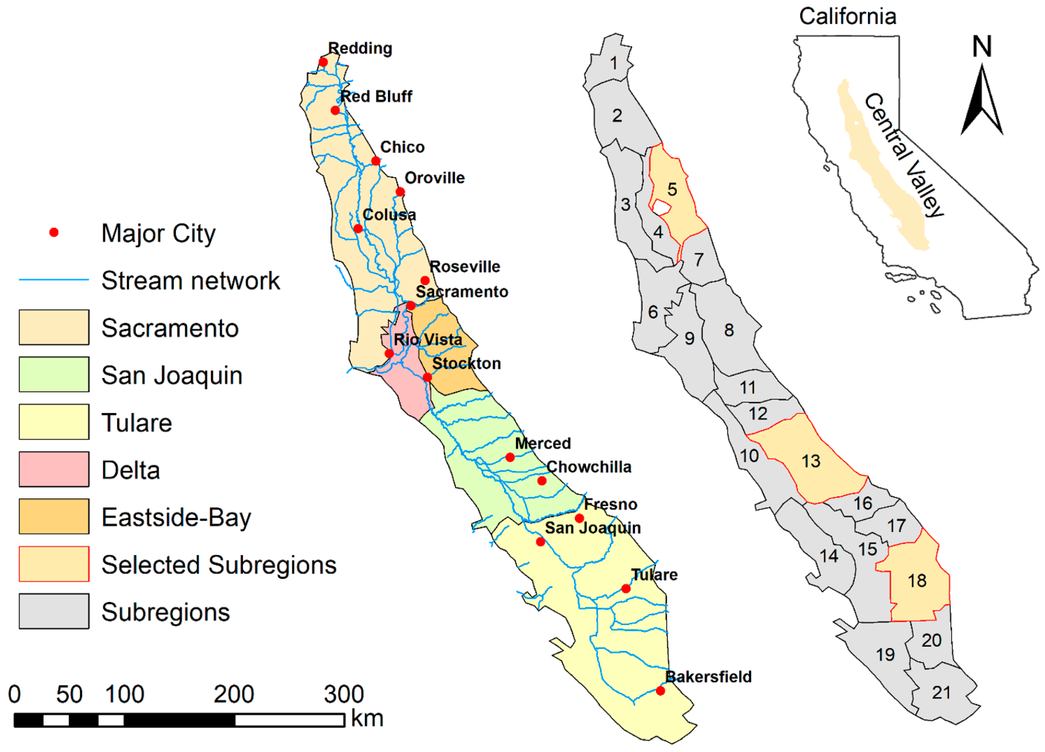
The CV consists of three major hydrologic regions (according to California Department of Water Resources [CDWR]), i.e., Sacramento, San Joaquin and Tulare (Figure 1), which is divided into 21 subregions by CDWR (Figure 1), where subregions 1 to 7 are in Sacramento, 11 to 13 in San Joaquin and 14 to 21 in Tulare. In this study, we focus on three subregions (one from each hydrologic region) for analyzing the nexus interaction, i.e., subregion 5, subregion 13 and subregion 18 (hereafter, referred as Sub-5, Sub-13 and Sub-18 respectively). These subregions are selected from different parts of CV to represent the diversity in climate (wetter north and drier south), water/energy supply and demand, cropping patterns, and irrigation practices.
The objective of this research is to use remote sensing and hydrologic models to assess the relationships between crops, energy and water as a nexus in the CV. To address this objective, the study aims to address the following questions: (i) how have the water and energy footprints changed over the past decade? and (ii) how do the dry and wet years impact the crop-energy-water relationships? We expect this study will (i) provide an insight into the evolution and interactions of selected nexus components, and (ii) demonstrate how remote sensing can help fill the gap in CEW nexus studies.
2. Materials and Methods
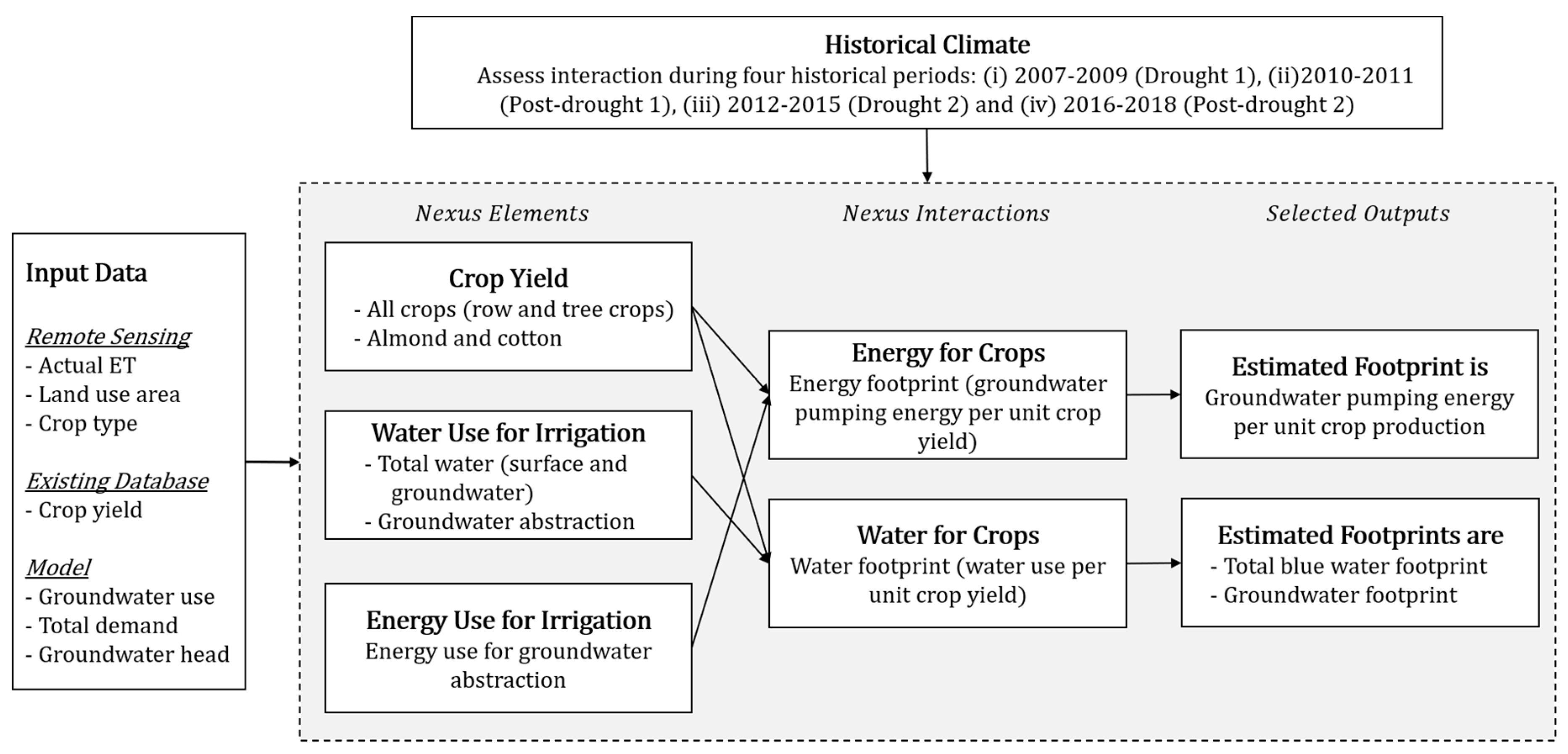
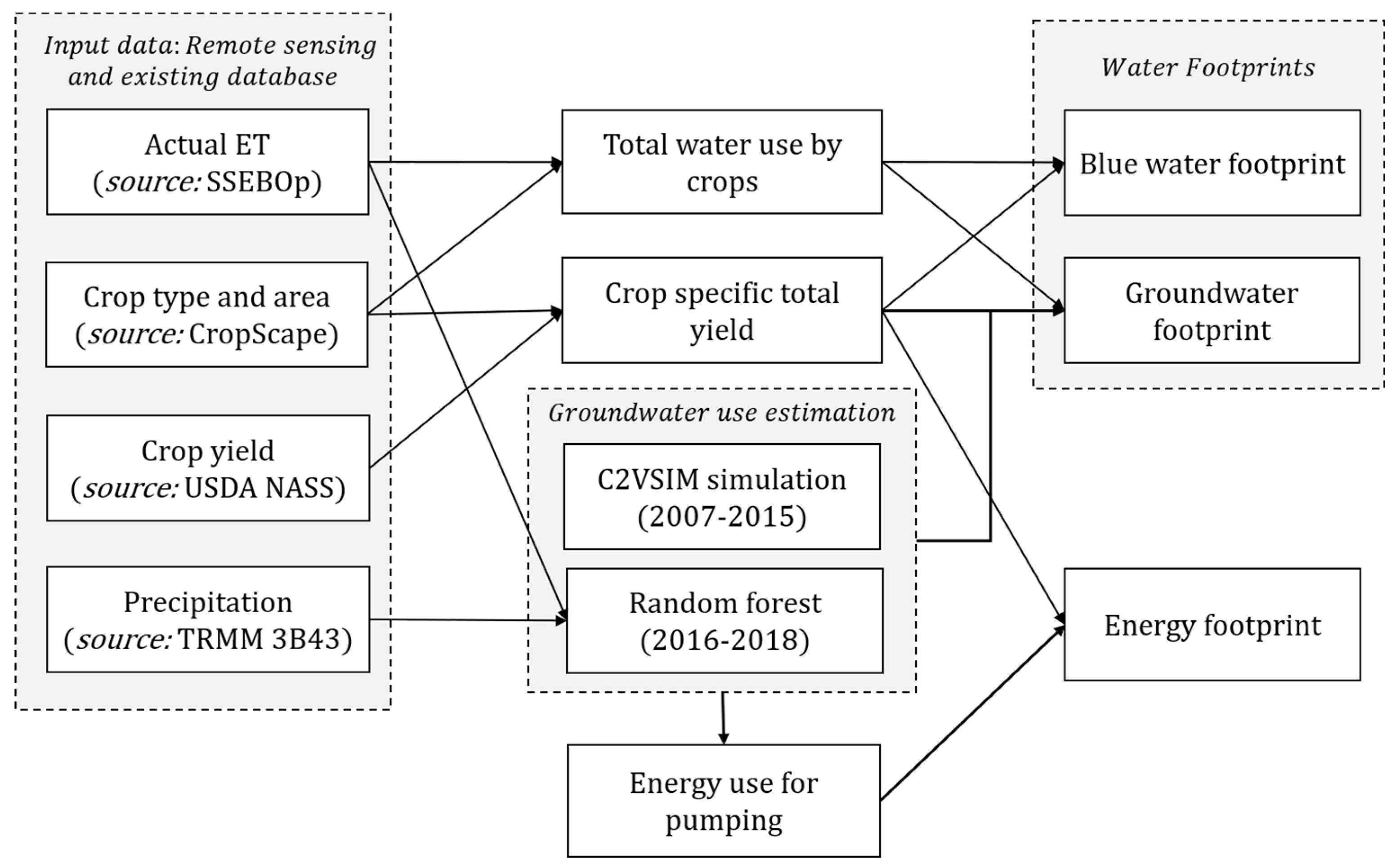
This section describes the detailed procedure used to identify the evolution and variability in the CEW nexus. The focused variables that we consider for assessing the nexus interactions include (i) crop yield (for all crops aggregated, almond and cotton), (ii) water use for irrigation (blue water), and (iii) energy use for groundwater pumping. We compare the historical changes (year 2007 to 2018) in the above three nexus components and analyze their relationships. Figure 2 shows a conceptual framework consisting of nexus components for this study. In the following subsections, we first describe the key data sources and then discuss the methods used to quantify the changes in CEW components. Finally, we show the steps followed to calculate (i) water use per unit crop yield (water footprint) and (ii) groundwater pumping energy use per unit crop yield (energy footprint) in the CV.
2.1. Data Collection
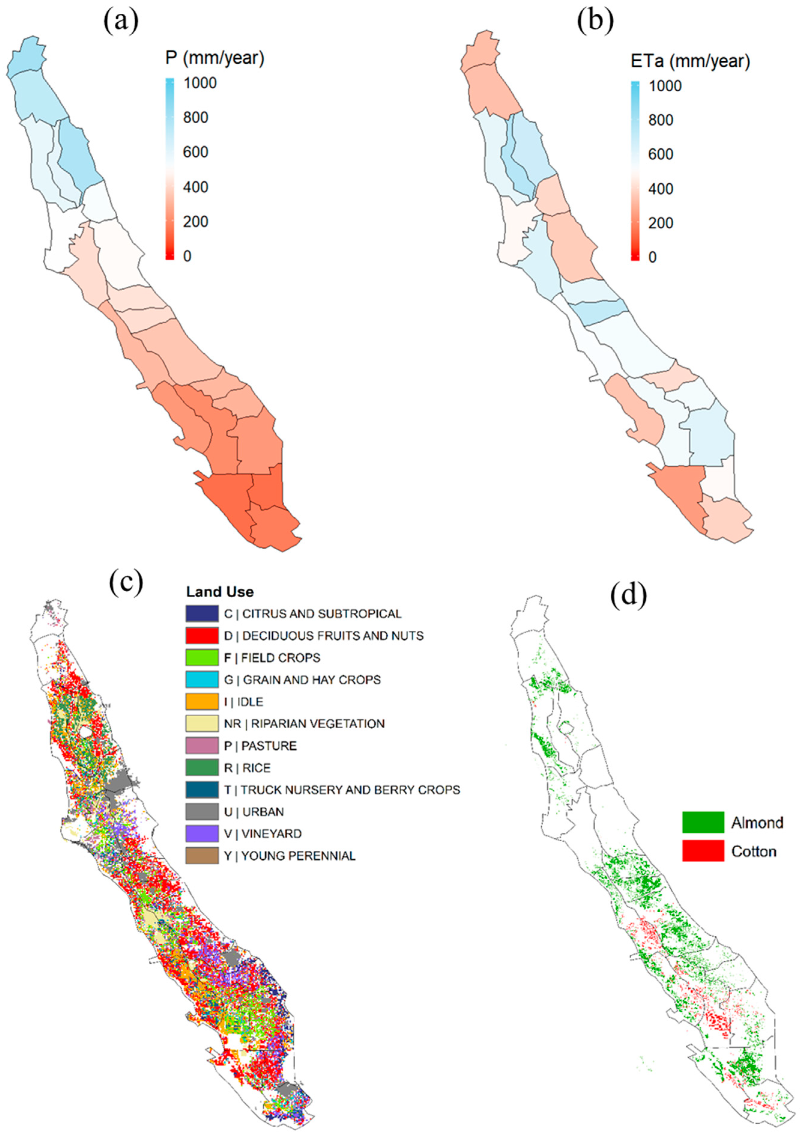
The study uses data from multiple sources (Table 1), with a focus on remote sensing products (i.e., precipitation, actual evapotranspiration, and cropping pattern) and numerical model outputs on groundwater use. Precipitation data is obtained from the Tropical Rainfall Measuring Mission (TRMM-3B43) [19]. TRMM-3B43 is a combined product of microwave satellite imagery from TRMM Microwave Imager (TMI), geostationary satellite infrared sensors, and rain gauges. The precipitation product has widely been applied in the field of hydrology, environment, water resources, meteorology, and agriculture, and has been validated by different projects [20,21,22]. We use the TRMM-3B43 product available at 0.25-degree (~27 km) resolution for the period of 2007–2018, which was then aggregated into each subregion to obtain average precipitation time series (Figure 3a). The actual evapotranspiration (ETa) is obtained from the Simplified Surface Energy Balance (SSEBop) model [23] for the same period. The SSEBop uses the Simplified Surface Energy Balance approach [24] that combines ET fractions derived from 1 km MODIS thermal imagery, which is based on similar principles adopted by SEBAL [25] and METRIC models [26]. We extract SSEBop-based ETa to estimate total water use in each subregion (Figure 3b).
The land use and crop type data used in this study are obtained from the U.S. Department of Agriculture, National Agricultural Statistics Service (USDA-NASS) Cropland Data Layer (CDL) [27]. The CDL is available through a web service CropScape [28]. USDA-NASS annually generates cropland layers over the entire U.S. at 30 m resolution (56 m for 2007 only). The CDL data is created using multiple satellite products including Landsat 5 Thematic Mapper (TM), Landsat 7 Enhanced TM Plus (ETM+), Advanced Wide Field Sensors (AWiFS), and Landsat 8 Operational Land Imager (OLI) [29,30,31,32]. The CDL provides spatially explicit crop type information with high spatial accuracy for major crops such as corn, soybeans and wheat [33]. The data is available for a limited time period over California (2007 to 2018). Figure 3c shows the spatial distribution of major cropping patterns in 2014, and Figure 3d highlights the spatial distribution of almond and cotton over CV. In general, most of the almond and cotton are produced in San Joaquin and Tulare regions. We extract crop areas for each crop type at the subregion level from the CDL dataset. Furthermore, we obtain crop yield information from the USDA-NASS existing database publicly available for California [34]. The crop yield information is available for more than 200 commodities on an annual basis (up to 2016) at the county level.
2.2. Crop Yield Estimation
The CV cropping patterns have been evolving in the past few decades. Here, we use crop yield for comparison among regions. There are more than 100 different types of crops cultivated in California with considerable regional variability. County-wide crop-specific yield (tons per acre) data in California are available at USDA-NASS [33]. The selected subregions primarily overlap Tulare County (Sub-18), Merced County (Sub-13) and Butte County (Sub-5). We use crop yield (tons per acre) data for each crop in the selected regions from the USDA-NASS database for the period of 2007 to 2016. We calculate the area of each crop type (individual and aggregated) from the CDL data (as described in the previous section) available for the period of 2007–2018. Total crop production (tons) for each crop is calculated from the product of yield (tons per km2) and the total crop area (km2) in each subregion. However, the land use data is available up to 2018, whereas the crop yield data is available up to 2016. For the extended period with no yield data (2017–2018), we assume the yield (tons/km2) is the same as the mean of last 2 years (2015–2016). In general, crop yield changes gradually in consecutive years except when there is exceptional climatic anomaly. Therefore, the assumption should facilitate a reasonable estimation of crop yield in the last 2 years of the study period (2017–2018).
2.3. Water Use Estimation
The water component of the nexus focuses on irrigation water use or blue water. Here, we use ETa to represent total crop water use, because more than 90% of annual ETa in the CV is supplied by irrigation (use groundwater and/or surface water sources) [35]. We also separate the total blue water use into surface water and groundwater components. To estimate groundwater use, we rely on the California Central Valley Groundwater-Surface Water Simulation Model (C2VSIM), which is a calibrated hydrological model capable of simulating detailed surface water and groundwater dynamics over the entire CV. The C2VSIM has been widely used for simulating surface water and groundwater dynamics in the CV, and the fine-grid version of the model simulation is available from October 1973 to September 2015 (see Ref. [36] for details about the C2VSIM model). We extract the surface water and groundwater use for irrigation in each subregion for the period (January 2007 to September 2015) and calculate the fraction of irrigation water supply coming from the groundwater, i.e., groundwater fraction (GF). The product of annual average GF and annual average ETa results in the actual evapotranspiration from groundwater irrigation. The GF after 2015 (years after C2VSIM simulation ends) is estimated using a linear regression model. The steps to develop the linear regression model and predict GF are as follows. First, we establish a linear regression model with annual groundwater abstraction as the dependent variable and GF as the independent variable. We use C2VSIM abstraction and derive GF for the period 2000–2015 to develop the regression model. Second, we use the groundwater abstraction (which is presented in detail in the following section) and the regression model to estimate GF for the recent data gap period (October 2015 to December 2018).
2.3.1. Estimate Groundwater Abstraction
The C2VSIM output on groundwater abstraction is only available until September 2015. To amend the data gap from then to the current time period (October 2015 to December 2018), we estimate the groundwater abstraction using a random forest regression model. The random forest regression technique has been widely applied for data classification and model fitting [37,38,39,40]. The method considers building an ensemble of random decision trees to create a ‘forest’, which can be trained with available datasets (a supervised algorithm). As the size of the tree grows, the data is randomly sampled at every node and the samples having the lowest mean squared error are retained [39]. Two important benefits of using the random forest technique are (i) flexible model structure that does not require pre-knowledge about data distribution, and (ii) relatively low computational cost [41]. These merits make the random forest an ideal model to estimate groundwater pumping with remote sensing products as predictor(s). The random forest model is established for each subregion on a monthly basis. We use precipitation and ETa as predictors and groundwater pumping rate (the monthly total withdrawal volume) as the response variable. The precipitation data is from TRMM-3B43 and actual evapotranspiration data from SSEBop, both of which are remote sensing products (see Section 2.1 for detail of the datasets). ETa is chosen because its variation directly corresponds to the agricultural demand. Since most of the precipitation occurs in the winter and almost none during the high demand period (summer), we experiment with different lag periods (0 to 7 month lag) and find precipitation with a 6-month lag sensitive to groundwater abstraction. This lag may be due to the fact that the winter streamflow is stored and released for irrigation in the summer, thus reducing the need for pumping to compensate the irrigation deficit. In addition, adding other potential variables like NDVI, potential evapotranspiration and crop area are found to not significantly contributable to the variability of groundwater pumping. The groundwater pumping rate for the period 2007–2015 is obtained from the C2VSIM output.
The random forest model is first calibrated and validated for the period January 2004 to December 2014, and is then used to estimate groundwater abstraction for the period with the data gap (October 2015 to December 2018). The performance of the random forest model is evaluated using Kling-Gupta efficiency (KGE) as shown in Equations (1) and (2). Although the stepwise linear regression model shows reasonable accuracy, we only choose the random forest for prediction.
where KGE is Kling-Gupta efficiency and CC is the Pearson correlation coefficient. c and r are computed and observed values; and are the standard deviations of computed and observed variables; and are the mean of estimated and available groundwater pumping rates respectively, and is the number of monthly time steps.
In addition to the estimation of groundwater abstraction for all crops (aggregated value for all crop scenario), we calculate groundwater abstraction for another two crops, i.e., almond and cotton. Since there is no spatially distributed abstraction data available for different crop types, we estimate the groundwater abstraction for the selected crop based on the fraction of total ETa of the crop. The calculation of ETa for a specific crop type is described below.
2.3.2. Estimate ETa for Specific Crops
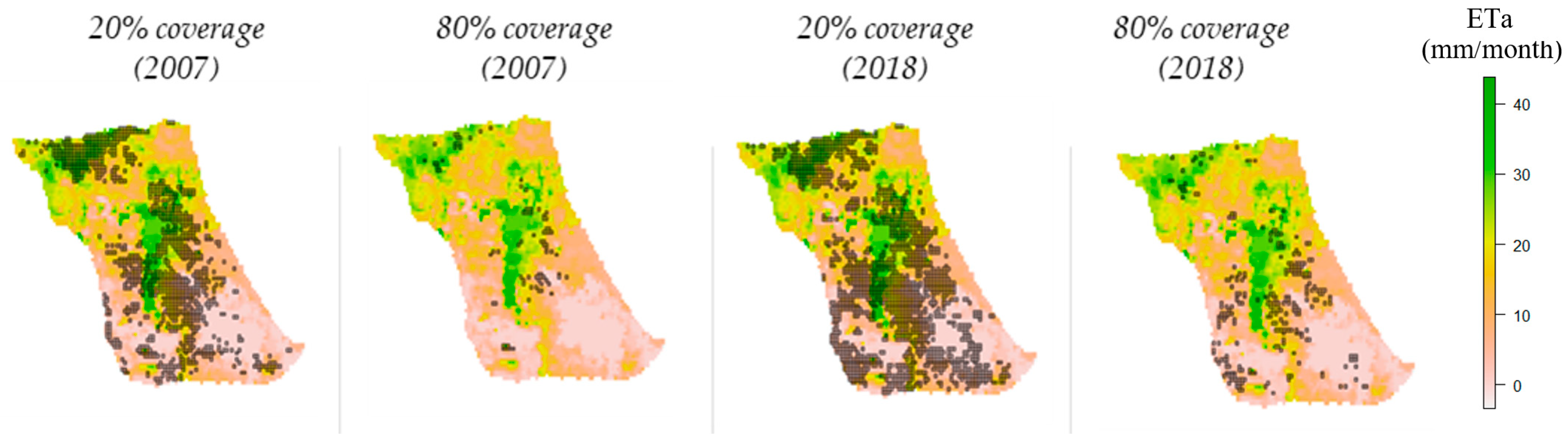
We use ETa to estimate water use for irrigation. The ETa data is extracted from a remote sensing product (SSEBop) at monthly time steps for the period of January 2007 to December 2018. Since the study focuses on agricultural water use, we extract ETa only for those SSEBop grid cells that are mostly covered by the crops of interest, the spatial extents of which come from the USDA-NASS CDL. However, there is a substantial difference in the resolutions of the ETa product (8 km) and land use data (30 m). We followed the following steps to resolve the discrepancy: (1) identify grids having more than 80% of crops (80% threshold selected to be on the conservative side); (2) calculate average ETa in the selected grids; and (3) estimate the total ETa volume using the product of the crop area and the ETa calculated in the previous step. In this study, we present analyses for aggregated crops (hereafter, all crops), almond (a highly profitable tree crop in California) and cotton (an important row crop in California). Figure 4 illustrates the selected ETa grids with different fractions of almond. The process is iterated for each year to estimate the crop-specific ETa in each year.
2.4. Energy Use Estimation
In general, energy consumption for groundwater pumping depends on several factors such as groundwater head, pump specification and efficiency, and the type of irrigation. However, it is difficult, if not impossible, to obtain most of the information at all locations for long time periods. Here, we use the average of energy used for per unit amount of groundwater pumping. Previous studies showed that the average energy use for groundwater pumping (average pumping efficiency is ~50%) is around 0.00051 kWh to lift 1 m3 of groundwater for 1 m [10]. Therefore, we use Equation (3) to estimate energy use for groundwater pumping, which is a function of the groundwater volume being pumped and the depth of groundwater (or lifting height). The process of estimating groundwater abstraction is discussed in the previous section. To estimate groundwater depth monthly, we follow these steps: (i) calculating the change in groundwater depth from the ratio of groundwater storage change (simulated by C2VSIM) and the area of the subregion (5, 13 and 18), and (ii) then compute cumulative groundwater depth using Equation (4).
where, is energy use for groundwater pumping (kWh), is the volume of groundwater being pumped (m3), and is the groundwater lifting height (m). GWs is the groundwater storage, is the month ( = 1 in first month of the estimation period), and denotes the area of the subregion. The initial depth of the groundwater table () is obtained from the previous study [42].
Since the C2VSIM output is available up to September 2015, we extrapolate the data into the rest of the study period (up to 2018). We apply the ordinary linear regression with groundwater pumping as the predictive variable and energy use as the dependent variable (at annual scale). The regression model shows a high coefficient of determination (R2 > 0.99). Therefore, we use the developed regression model to estimate energy use for an extended time period (October 2015 to December 2018).
2.5. Water and Energy Footprints Estimation
Water footprint assessment [43] provides an estimate of consumptive water use for different crops. In the agricultural context, consumptive water use includes the water from managed irrigation source (or “blue water”) and effective rainfall (or “green water”). In this study, we report blue water footprint for all crops (aggregated), almond and cotton. In general, green water accounts for less than 10% of the consumptive use [8], and the majority of the consumptive water comes from blue water. This is primarily because the rain occurs during winters but water demand for cropping peaks in late springs and summers. Surface water stored in headwater reservoirs in the winters is released and delivered for irrigation during high-demand periods, whereas additional irrigation deficit is satisfied by groundwater. In general, blue water footprint (BWF) varies with cropping patterns, farming decisions, climate, and crop response. The BWF is calculated using a similar method to that used in Reference [43] as shown in Equation (5). By providing evapotranspiration coming from groundwater and surface water, the BWF component coming from each water sources can be determined. The Equations (5) and (6) are used for calculating total Blue Water Footprint (BWF) and Groundwater Footprint (GWF).
where, annual ETa (actual evapotranspiration) is in m3 and crop yield is in tons, the unit of BWF (or GWF) is m3 of water per ton of crop yield, and is the groundwater component of total water used by crops.
Similar to the water footprint, we calculate the energy footprint for all crops (aggregated), almond and cotton. The energy footprint for this study is the amount of groundwater pumping energy (kWh) required annually to produce crops per ton. The Equation (7) shows the formula of energy footprint (EF).
In addition, we calculate the amount of energy used per unit volume of groundwater abstraction (EGA). The value of EGA provides a useful measure for understanding relative stress on the energy sector for groundwater abstraction (Equation (8)).
In sum, an illustration of the steps used to calculate the water and energy footprint using remotely sensed data and existing database is shown in Figure 5. A detailed description of the methodology has been presented in this and above in other sections.
3. Results and Discussion
3.1. Historical Precipitation and Cropping Patterns
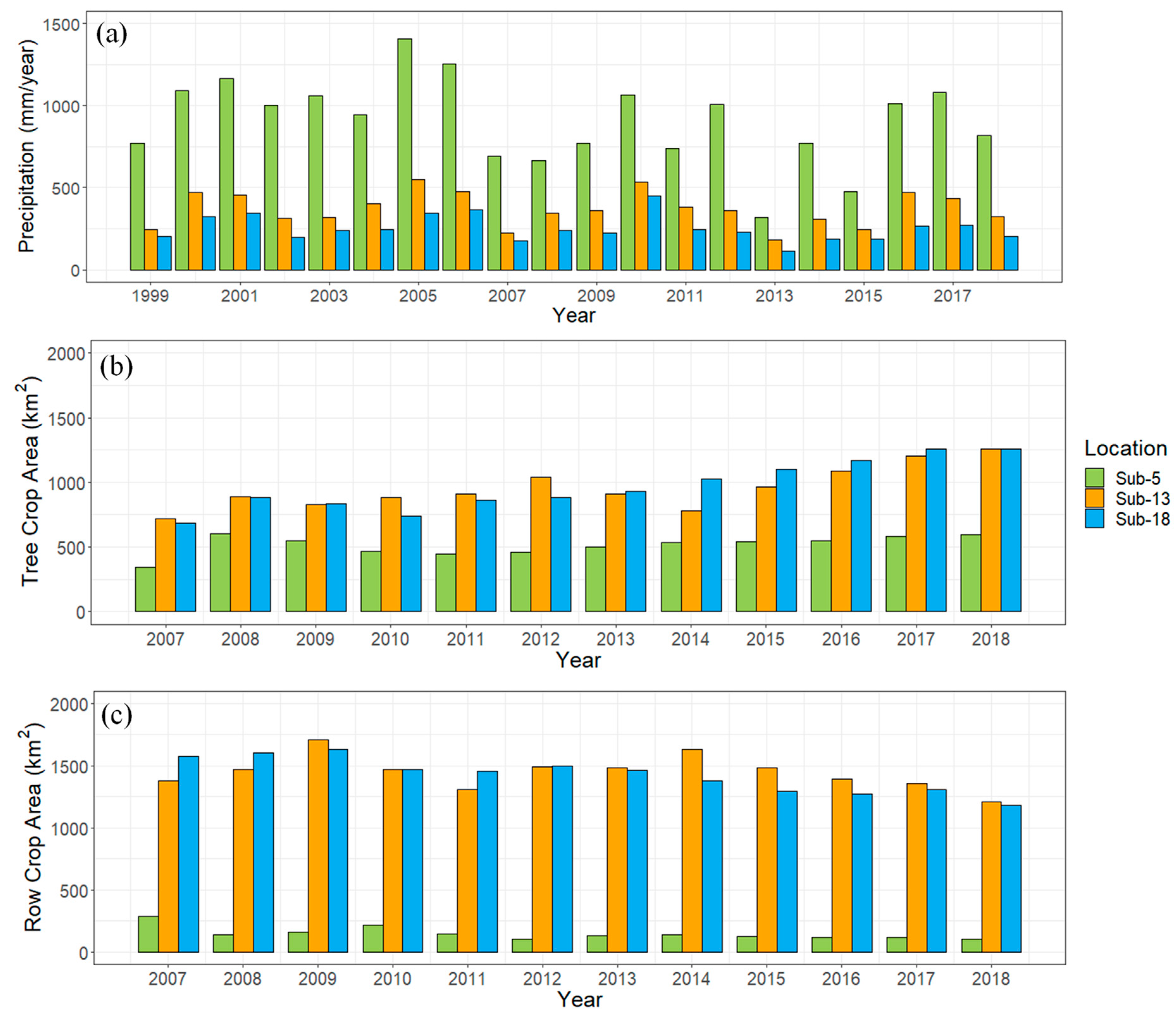
Climate plays important roles in shaping the agricultural production, energy production (hydropower) and use, and surface water-groundwater distribution. In general, there exists a north–south precipitation gradient with higher precipitation in the north (due to large amount of moisture from westerly winds) and relatively lower in the south [44]. A series of droughts in the past decade critically stressed the CV. The annual precipitation over Sacramento (Sub-5), San Joaquin (Sub-13) and Tulare (Sub-18) for the period of 1999 to 2018 is shown in Figure 6a. The precipitation was relatively lower during the two major droughts which occurred in the periods of 2007–2009 and 2012–2015. Other than drought periods, there were also a few wet periods like year 2005, 2010 and 2017.
The crop distribution in the CV has been evolving in the past decades. We calculate the area of row crops and tree crops from the USDA-NASS (discussed in Section 2.1) for the period 2007–2018, and the crop patterns prior to the period are obtained from C2VSIM model inputs. In general, there has been a downward trend in row crops and an upward trend in high-value tree crops (Figure 6b,c). Sub-13 has more farmland than the other two subregions. Tree crops generally have an increasing trend in Sub-13. In all cases, row crops have a general decreasing trend. Despite multiple drought events in the past decade, the crop area of high-value tree crops continues to increase. Tree crops exert extra pressure on groundwater resources especially during droughts [9], as tree crops cannot be fallowed like row crops and must be irrigated without interruption to sustain production. Tree crops like almond and pistachio nuts bring greater economic return, which lead farmers to prefer these over other traditional crops like cotton.
3.2. Historical Changes in Groundwater Use
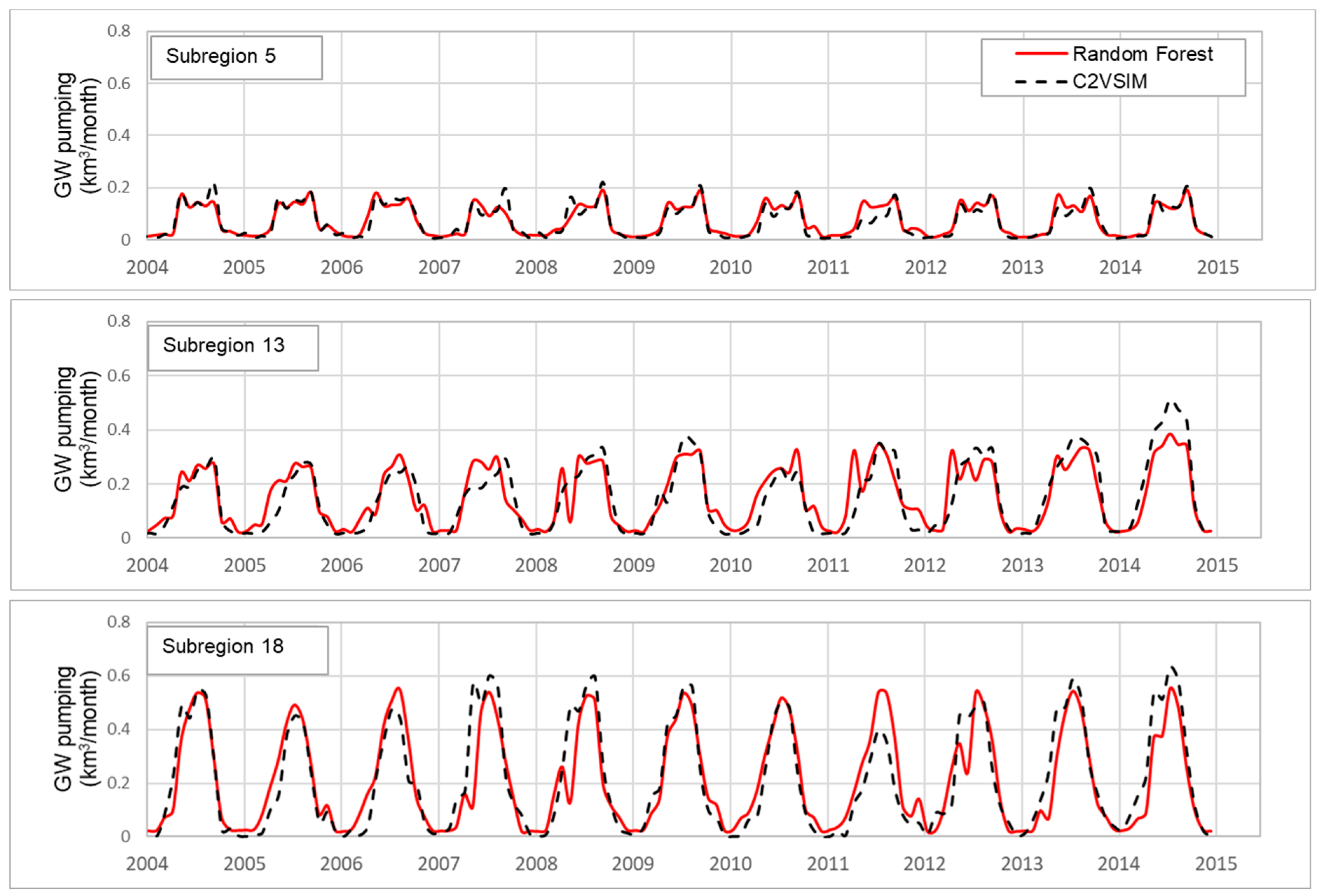
As described in Section 2.3.1, groundwater pumping information is required to estimate (1) the fraction of water use that originates from groundwater, and (2) the energy used for groundwater pumping. Figure 7 shows the estimated vs C2VSIM groundwater abstraction for three subregions at monthly time scale. The model has been calibrated for multiple periods between January 2004 to September 2015, which includes both dry and wet years (calibration for years 2004–2006, 2009–2010, and 2013–2014, and validation for the rest years). The Kling-Gupta Efficiency (KGE) for subregions 5, 13 and 18 are 0.91, 0.81 and 0.88 respectively for the calibration periods, and 0.85, 0.80 and 0.79 respectively for the validation periods. The KGE values for the selected subregions are reasonable, indicating the method can be used to predict the groundwater abstraction for the data gap period of October 2015 to December 2018. The period of 2016 to 2018 is relatively wet when the model is expected to provide a reasonable estimate, as we found that the model performs better during normal (years having average precipitation) and wet years (Figure 7). For any calculation involving groundwater abstraction, we use C2VSIM abstraction estimation up to September 2015 and predict values (using the developed model) for the period of October 2015 to December 2018.
3.3. Spatial and Temporal Variation in Water Footprints
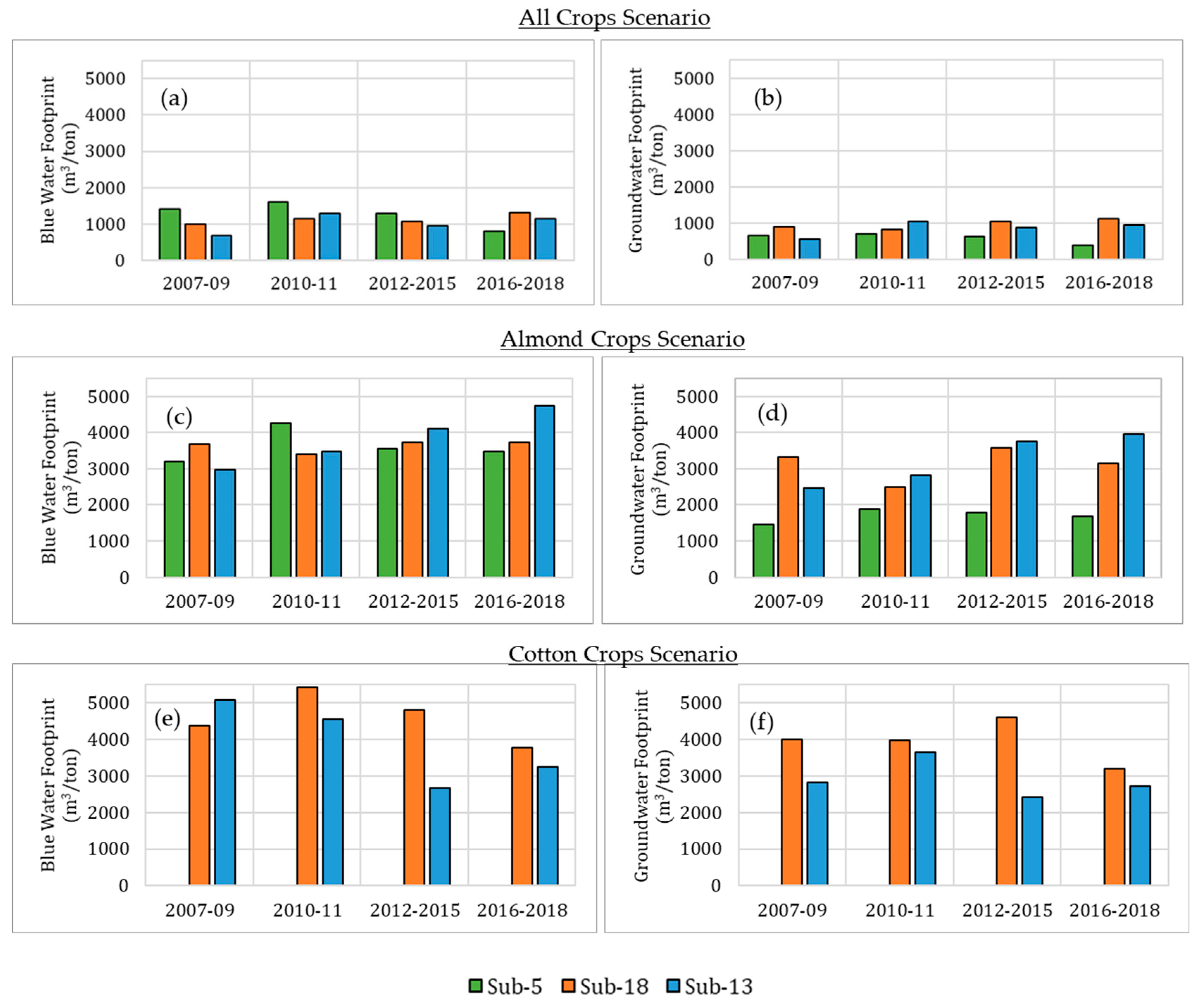
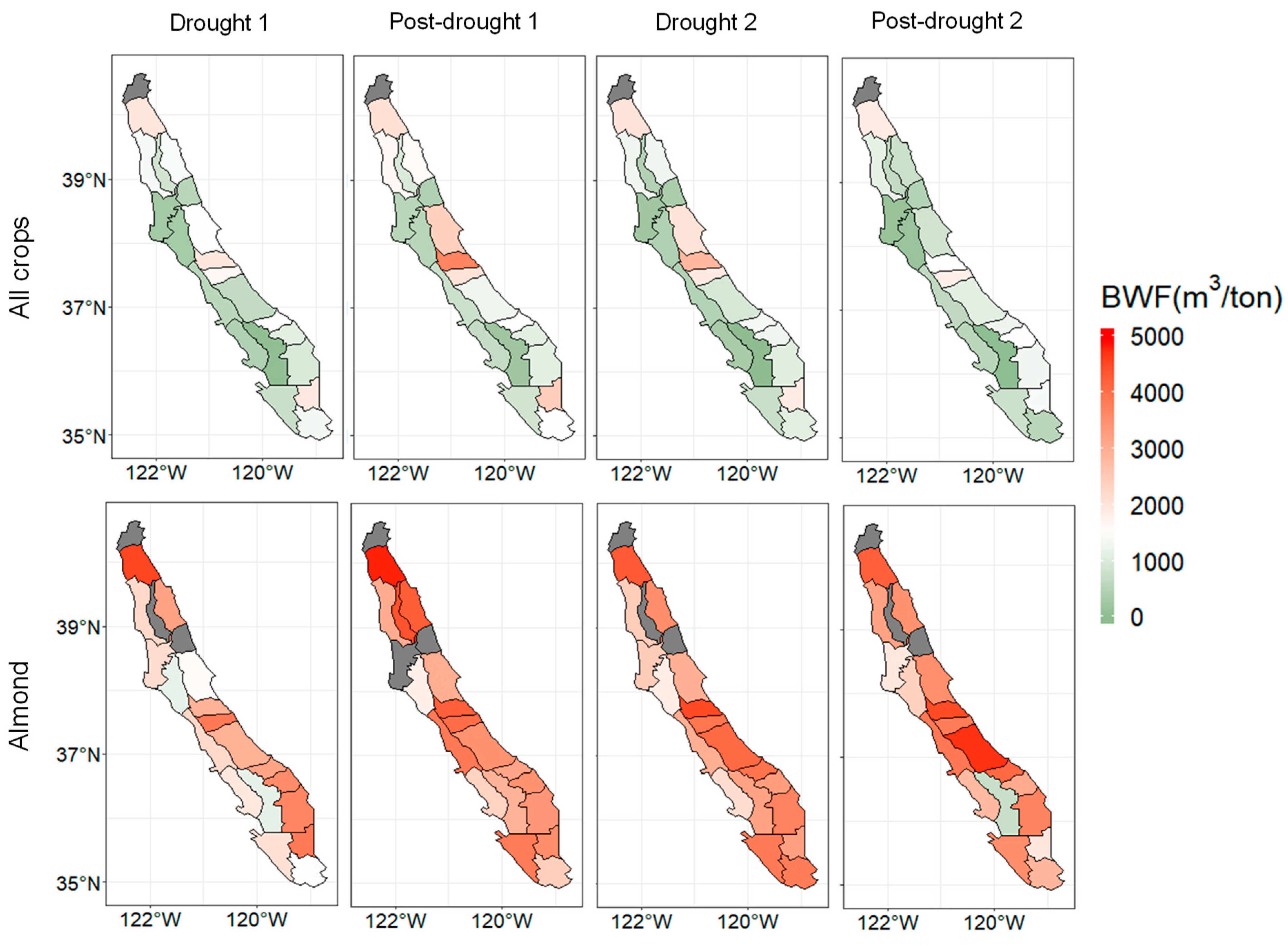
BWFs and GWFs for three crop scenarios (all crops averaged, almond and cotton) in Sacramento (Sub-5), San Joaquin (Sub-13) and Tulare (Sub-18) are shown in Figure 8. We compare the footprints for four historical periods, i.e., drought 1 (2007–2009), post-drought 1 (2010–2011), drought 2 (2012–2015) and post-drought 2 (2016–2018). Comparisons between the two drought periods and wet periods allow us to understand the characteristics of BWFs and GWFs under extreme and moderate scenarios. Based on the historical BWF estimates under all crop-averaged scenarios, (Figure 8a) we find (i) in Sub-5, that the BWFs show a decreasing trend irrespective of drought years (the BWF during post-drought 2 is almost half of that during post-drought 1), which indicates increased water use efficiency; (ii) in contrast, the BWF in Sub-13 are higher during post-droughts than the drought periods, where the BWF in post-drought 1 (~1300 m3/ton) is around twice compared to drought 1 (~672 m3/ton) and higher in post-drought 2 than drought 2; and (iii) the BWF in Sub-18 gradually increases (around 331 m3/ton higher BWF in post-drought 2 compared to drought 1), which may be due to decreased crop yield, increased water use (due to warmer temperature), or lower water use efficiency. Moreover, we compare the spatial distribution of BWFs (Figure 9), which shows that BWFs in subregion 8, 11, 12, and 20 are relatively higher than that in other subregions.
Similar to the BWF, a comparison of GWFs among selected regions and for different scenarios is shown in Figure 8b. Based on the GWF estimates under all crop scenarios, we find (i) on average, BWFs are around 110%, 20% and 20% higher than GWFs in Sub-5, Sub-18 and Sub-13 respectively, indicating higher groundwater dependency in Sub-13 and Sub-18 compared to higher surface water dependency in Sub-5; and (ii) the trend and interannual variability patterns in GWF are similar to those in BWF, i.e., Sub-5 shows a decreasing trend, Sub-18 shows an increasing trend and Sub-13 has higher GWF during post-droughts. Although total harvested area has decreased during past droughts (173,200 hectares cropland fallowed in 2014), the GWF increased in the southern CV [8]. Such an increase can be attributed to a shift towards high water intensive crops (fruits, nuts and vineyards) and continuously increasing temperature.
We compare the BWF and GWF of almond crop for the study regions in Figure 8c,d. The BWF for almond is on average around 30% higher than the BWF under all crops scenario. Average BWF for almond is 3556 m3/ton and GWF is 2167 m3/ton (averaged over three study subregions and periods). A previous study [45] found that the BWF for almond in 2011 is 3652 m3/ton, which is very close to our estimate. Based on the water footprint estimation (BWF and GWF) for almond crops, we find (i) in Sub-5, water footprints (both BWF and GWF) are relatively higher during post-drought 1, but about similar during other periods, indicating relatively stable water use efficiency in Sub-5; (ii) Sub-18 shows relatively higher sensitivity to droughts (especially GWF), where GWFs during drought 1 and drought 2 are around 33% and 44% higher than post-drought 1; (iii) in Sub-13, water footprints (both BWF and GWF) gradually increase throughout the historical period, where the GWF during post-drought 2 is around 60% higher than drought 1; and (iv) on average, the GWFs in Sub-18 and Sub-13 are around 84% and 92% higher than that of Sub-5 respectively. The increasing GWF in Sub-13 is higher than Sub-18 during drought 2 and later, indicating higher water stress in the southern part of the CV. Additionally, we compare the spatial distribution of BWF of almond (Figure 9) and find that the BWFs of almond have increased in most of the subregions during the recent study period. During post-drought 2, BWF is relatively higher in Sub-11 and Sub-13. Moreover, we also compare BWFs and GWFs of cotton crops (Figure 8e,f) for Sub-18 and Sub-13 (Sub-5 is not considered due to a lack of explicit cotton grids, see Figure 3d). We find that the BWFs during the later periods (drought 2 and post-drought 2) are relatively lower. On average, the BWF in Sub-18 is around 1.18 times as much as that in Sub-13. The GWF in Sub-18 is relatively higher during droughts (17% higher than average during drought 2), whereas the GWF in Sub-13 is relatively stable but higher during post-drought 1 (26% higher than average). On average, the BWF of cotton is around 3.7 times as much as the BWF of all crops scenario.
3.4. Spatial and Temporal Variation in Energy Footprints
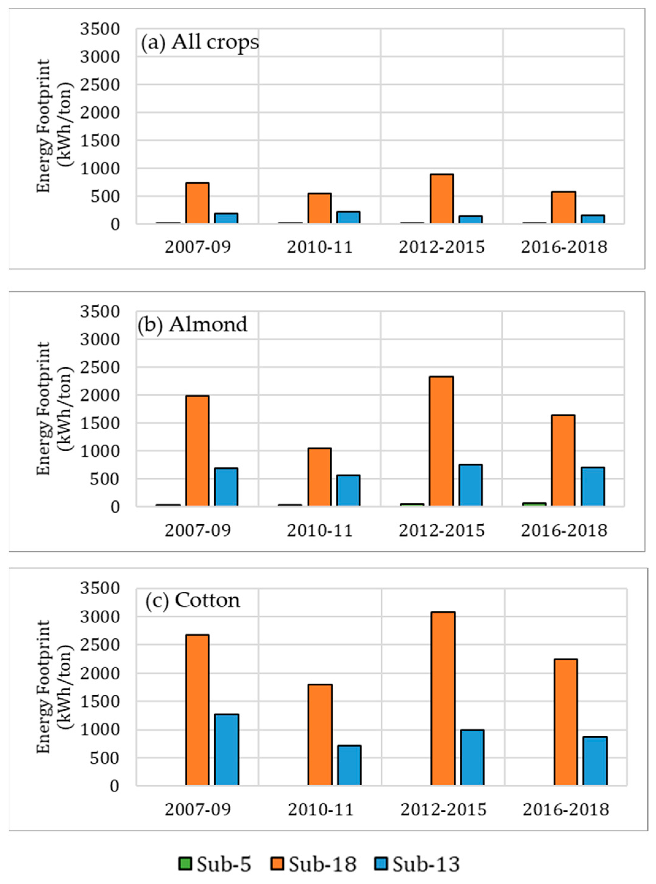
EFs under three cropping scenarios in three selected subregions are shown in Figure 10. Similar to water footprints shown in the previous section, climate remains an important driver to affect the spatiotemporal patterns of EFs. Based on the historical EFs, spatially we find that the EF under all crops scenario in Sub-18 is around 4 and 40 times as much as Sub-13 and Sub-5 respectively. EF under almond crop scenario in Sub-18 is around 2.6 and 35 times as much as Sub-13 and Sub-18 respectively. Furthermore, the EF in Sub-18 under cotton crop scenario is around 2.5 times as much as Sub-13. The high value of EF in Sub-18 may be explained by a high volume of groundwater abstraction and greater lifting height. Temporally, in all cases, EF is highest during drought 2, indicating the greatest stress brought by the most recent drought on energy supply for groundwater pumping. On average, EFs under almond crop and cotton crop scenarios are around 3 and 3.9 times as much as the EF under all crops scenario.
3.5. Spatial and Temporal Variation in Energy Use for Water
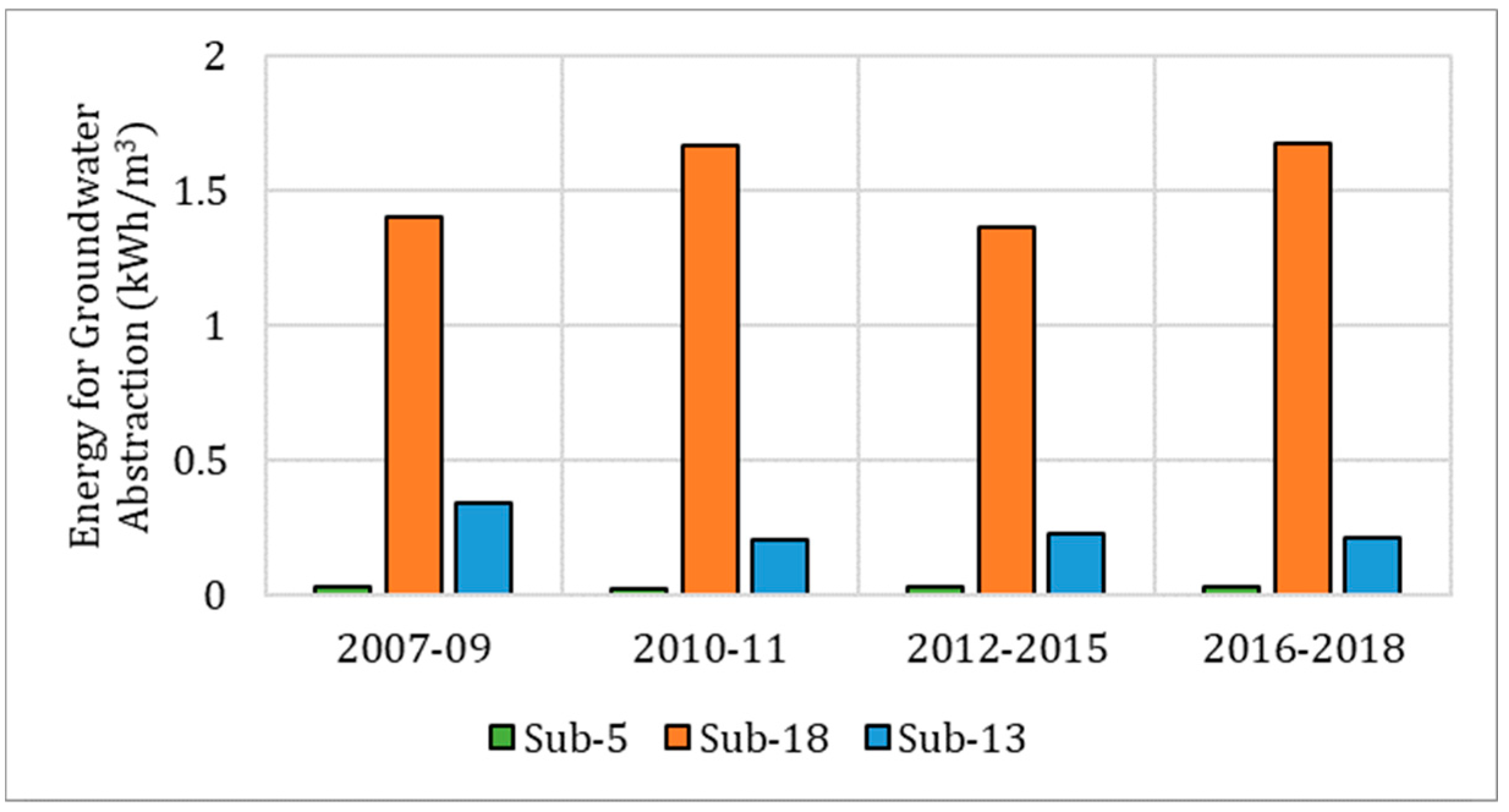
In addition to the estimation of water and energy footprints, we compute the EGA in the selected subregions (Figure 11). The average EGA in Sub-5, Sub-18 and Sub-13 are 0.03 kWh/m3, 0.66 kWh/m3 and 0.25 kWh/m3 respectively. The highest EGA in Sub-18 is due to its greatest lifting height as described before. The interannual variability in EGA in Sub-18 is the highest with relatively greater magnitude during post-droughts. On average, the EGA in Sub-13 is around 63% lower than that in Sub-18. In addition, the amount of energy used per unit of groundwater abstraction in Sub-13 is relatively lower in the later years than its beginning (drought 1), which indicates increased groundwater use efficiency. Furthermore, the average EGA in Sub-5 is around 95% lower than that in Sub-18. The lower EGA in the northern region (Sub-5) is attributed to the lower lifting height for groundwater pumping (due to the relatively shallower groundwater level).
4. Conclusions
An understanding of the CEW nexus in the agriculture sector is critical to improve natural resources management in agricultural regions. In this study, we assess the CEW nexus in three subregions of Central Valley, i.e., Sacramento (subregion 5), San Joaquin (subregion 13) and Tulare (subregion 18), which have distinct water availability conditions. The specific nexus elements considered include water use (blue water) and energy use for groundwater pumping, and crop production (all crops, almond and cotton). To characterize the CEW nexus, we use remote sensing, hydrologic models and machine learning techniques to quantify two nexus metrics, inlcuding (i) water use for crops (water footprint) and (ii) energy use for crops (energy footprint). The results of this study are presented over four historical periods having diverse climatic conditions, including Drought 1 (2007–2009), Post-drought 1 (2010–2011), Drought 2 (2012–2015), and Post-drought 2 (2016–2018). Based on the results, we conclude that:
- The Central Valley has experienced increased stress of water and energy supplies to meet ever-increasing agricultural demand, which was worsened during the two major droughts in the past decade. The highest impact (negative) of droughts occurred in water-scarce southern regions, San Joaquine and Tulare. The GWFs of high water consumptive tree crop (almond) in Tulare and San Joaquine are around 84% and 92% higher than those in Sacramento on average.
- The water footprint of almond in recent years is higher than almost all other crops. The total blue water footprint for almond has been increasing, with the highest increasing rate in San Joaquine. In contrast, the total blue water footprint for cotton has decreased in recent years. The groundwater footprint in Tulare increased during both droughts (with the highest magnitude during the most recent megadrought). Groundwater footprint in Sacramento is relatively less than that in the other subregions, but has a modest increasing trend.
- The energy footprint (energy for groundwater pumping) for all crops scenario in Tulare is substantially higher than other regions. For almond and cotton, both Tulare and San Joaquine subregions have higher energy footprints than the scenario of all crops. On average, energy footprints under almond and cotton crops are around 3 to 3.9 times as much as the energy footprint under all crops scenario.
In this study, remote sensing is used to parameterize factors (e.g., precipitation, ETa, and cropping area) that are critical to characterize the CEW nexus in spatially and temporally explicit manners over a broad agricultural region, Central Valley. For example, both precipitation and evapotranspiration are important components of the hydrologic cycle, and their magnitude and spatial patterns will affect the availability of surface water supplies and thereby differential groundwater footprints and energy footprints related to pumping. Although the results are aggregated and analyzed at the subregion level in this paper, remote sensing allows more spatially and temporally detailed inquiry into the CEW nexus in variable scales. The methodology framework introduced in this paper may be transferrable to other agriculturally important regions (e.g., the U.S. High Plains Aquifer) for the characterization of the CEW nexus across different spatial and temporal scales.
Author Contributions
Conceptualization, M.G. and R.L.; methodology, S.A.; formal analysis, S.A. and R.L.; investigation, S.A. and M.G.; resources, M.G.; data curation, S.A.; writing—original draft preparation, S.A.; writing—review and editing, R.L.; visualization, S.A.; supervision, M.G.; funding acquisition, M.G.
Funding
This research was funded by The University of California Research Initiatives Award, grant number LFR-18-548316.
Acknowledgments
We are grateful to Tariq Kadir and Emin Dogrul from California’s Department of Water Resources for technical assistance in the use of C2VSIM.
Conflicts of Interest
The authors declare no conflict of interest. The funders had no role in the design of the study; in the collection, analyses, or interpretation of data; in the writing of the manuscript, or in the decision to publish the results.
References
- United Nations (UN) 2015 Transforming Our World: The 2030 Agenda for Sustainable Development. Available online: https://sustainable development.un.org/post2015/transformingourworld (accessed on 12 May 2019).
- Lawford, R.; Bogardi, J.; Marx, S.; Jain, S.; Wostl, C.P.; Knuppe, K.; Ringler, C.; Lansigan, F.; Meza, F. Basin perspectives on the water–energy–food security nexus. Curr. Opin. Environ. Sustain. 2013, 5, 607–616. [Google Scholar] [CrossRef]
- Howells, M.; Hermann, S.; Welsch, M.; Bazilian, M.; Segerström, R.; Alfstad, T.; Gielen, D.; Rogner, H.; Fischer, G.; Van Velthuizen, H.; et al. Integrated analysis of climate change, land-use, energy and water strategies. Nat. Clim. Chang. 2013, 3, 621. [Google Scholar] [CrossRef]
- Scott, C.A. The water-energy-climate nexus: Resources and policy outlook for aquifers in Mexico. Water Resour. Res. 2011, 47. [Google Scholar] [CrossRef] [Green Version]
- Smajgl, A.; Ward, J.; Pluschke, L. The water–food–energy Nexus–Realizing a new paradigm. J. Hydrol. 2016, 533, 533–540. [Google Scholar] [CrossRef]
- Biggsa, E.M.; Bruceb, E.; Boruffc, B.; Duncana, J.M.; Horsleyc, J.; Paulic, N.; McNeilld, K.; Neefd, A.; Ogtrope, F.V.; Curnowf, J.; et al. Imanarig Sustainable development and the water–energy–food nexus: A perspective on livelihoods. Environ. Sci. Policy 2015, 54, 389–397. [Google Scholar] [CrossRef]
- Maupin, M.; Kenny, J.; Hutson, S.; Lovelace, J.; Barber, N.; Linsey, K. Estimated Use of Water in the United States in 2010; U.S. Geological Survey: Reston, VA, USA, 2014; Volume 1405, p. 53.
- Howitt, R.; Medellın-Azuara, J.; MacEwan, D.; Lund, J.; Sumner, D. Economic Analysis of the 2014 Drought for California Agriculture; University of California, Davis-Center for Watershed Sciences: Yolo, CA, USA, 2014. [Google Scholar]
- Xiao, M.; Koppa, A.; Mekonnen, Z.; Pagán, B.R.; Zhan, S.; Cao, Q.; Aierken, A.; Lee, H.; Lettenmaier, D.P. How much groundwater did California’s Central Valley lose during the 2012–2016 drought? Geophys. Res. Lett. 2017, 44, 4872–4879. [Google Scholar] [CrossRef]
- Dale, L. Quantifying Groundwater Pumping Energy Use and Costs in California to Improve Energy and Water Systems Reliability; ETA Seminar, Lawrence Berkeley National Laboratory Technical report; University of California, Davis-Center for Watershed Sciences: Yolo, CA, USA, 2016. [Google Scholar]
- Diffenbaugh, N.S.; Swain, D.L.; Touma, D. Anthropogenic warming has increased drought risk in California. Proc. Natl. Acad. Sci. USA 2015, 112, 3931–3936. [Google Scholar] [CrossRef] [Green Version]
- Mubako, S.T.; Lant, C.L. Agricultural virtual water trade and water footprint of U.S. States. Ann. Assoc. Am. Geogr. 2013, 103, 385–396. [Google Scholar] [CrossRef]
- Mekonnen, M.; Hoekstra, A. The green, blue and grey water footprint of crops and derived crop products. Hydrol. Earth Syst. Sci. 2011, 15, 1577–1600. [Google Scholar] [CrossRef] [Green Version]
- Fulton, J.; Cooley, H.; Gleick, P.H. California’s Water Footprint; Technical Report; Pacific Institute: Oakland, CA, USA, 2012. [Google Scholar]
- Fulton, J.; Cooley, H.; Gleick, P.H. Water footprint outcomes and policy relevance change with scale considered: Evidence from California. Water Resour. Manag. 2014, 28, 3637–3649. [Google Scholar] [CrossRef]
- Mubako, S.T.; Lahiri, S.; Lant, C.L. Input-output analysis of virtual water transfers: Case study of California and Illinois. Ecol. Econ. 2013, 93, 230–238. [Google Scholar] [CrossRef]
- Marston, L.; Konar, M. Drought impacts to water footprints and virtual water transfers of the Central Valley of California. Water Resour. Res. 2017, 53, 5756–5773. [Google Scholar] [CrossRef]
- CPUC (California Public Utilities Commission). Embedded Energy in Water Studies: Study 3 End-Use Water Demand Profiles; California Public Utilities Commission: San Francisco, CA, USA, 2011. Available online: ftp://ftp.cpuc.ca.gov/gopherdata/energy%20efficiency/Water%20Studies%203/End%20Use%20Water%20Demand%20Profiles%20 Study%203%20FINAL.PDF (accessed on 27 April 2017).
- Huffman, G.J.; Bolvin, D.T.; Nelkin, E.J.; Wolff, D.B.; Adler, R.F.; Gu, G.; Hong, Y.; Bowman, K.P.; Stocker, E.F. The TRMM multisatellite precipitation analysis (TMPA): Quasi-global, multiyear, combined-sensor precipitation estimates at fine scales. J. Hydrometeorol. 2007, 8, 38–55. [Google Scholar] [CrossRef]
- Li, X.-H.; Zhang, Q.; Xu, C.-Y. Suitability of the TRMM satellite rainfalls in driving a distributed hydrological model for water balance computations in Xinjiang catchment, Poyang lake basin. J. Hydrol. 2012, 426, 28–38. [Google Scholar] [CrossRef]
- Sahoo, A.K.; Sheffield, J.; Pan, M.; Wood, E.F. Evaluation of the tropical rainfall measuring mission multi-satellite precipitation analysis (TMPA) for assessment of large-scale meteorological drought. Remote Sens. Environ. 2015, 159, 181–193. [Google Scholar] [CrossRef]
- Zhang, A.; Jia, G. Monitoring meteorological drought in semiarid regions using multi-sensor microwave remote sensing data. Remote Sens. Environ. 2013, 134, 12–23. [Google Scholar] [CrossRef]
- Senay, G.B.; Budde, M.; Verdin, J.P. Enhancing the Simplified Surface Energy Balance (SSEB) approach for estimating landscape ET: Validation with the METRIC model. Agric. Water Manag. 2011, 98, 606–618. [Google Scholar] [CrossRef]
- Senay, G.B.; Bohms, S.; Singh, R.; Gowda, P.A.; Velpuri, N.M.; Alemu, H.; Verdin, J.P. Operational evapotranspiration mapping using remote sensing and weather datasets: A new parameterization for the SSEB approach. J. Am. Water Resour. Res. 2013, 49, 577–591. [Google Scholar] [CrossRef]
- Bastiaanssen, W.G.M.; Menenti, M.; Feddes, R.A.; Holtslag, A.A.M. The surface energy balance algorithm for land (SEBAL): Part 1 formulation. J. Hydrol. 1998, 212–213, 198–212. [Google Scholar] [CrossRef]
- Allen, R.G.; Tasumi, M.; Trezza, R. Satellite-based energy balance for mapping evapotranspiration with internalized calibration (METRIC–Model. ASCE J. Irrig. Drain. Eng. 2007, 133, 380–394. [Google Scholar] [CrossRef]
- USDA NASS CDL. CropScape–Cropland Data Layer. 2018. Available online: https://nassgeodata.gmu.edu/CropScape (accessed on 5 March 2019).
- Han, W.; Yang, Z.; Di, L.; Zhang, B.; Peng, C. Enhancing agricultural geospatial data dissemination and applications using geospatial Web services. IEEE J. Sel. Top. Appl. Earth Obs. Remote Sens. 2014, 7, 4539–4547. [Google Scholar] [CrossRef]
- Boryan, C.; Yang, Z.; Mueller, R.; Craig, M. Monitoring US agriculture: The US Department of Agriculture, National Agricultural Statistics Service, Cropland Data Layer Program. Geocarto Int. 2011, 26, 341–358. [Google Scholar] [CrossRef]
- Daggupati, P.; Douglas-Mankin, K.R.; Sheshukov, A.Y.; Barnes, P.L.; Devlin, D.L. Field-level targeting using SWAT: Mapping output from HRUs to fields and assessing limitations of GIS input data. Trans. ASABE 2011, 54, 501–514. [Google Scholar] [CrossRef]
- Johnson, D.M. A 2010 map estimate of annually tilled cropland within the conterminous United States. Agric. Syst. 2013, 114, 95–105. [Google Scholar] [CrossRef]
- Stern, A.; Doraiswamy, P.C.; Hunt, E.R. Changes of crop rotation in Iowa determined from the United States Department of Agriculture, National Agricultural Statistics Service cropland data layer product. J. Appl. Remote Sens. 2012, 6, 063590. [Google Scholar] [CrossRef]
- Han, W.; Yang, Z.; Di, L.; Mueller, R. CropScape: A Web service-based application for exploring and disseminating US conterminous geospatial cropland data products for decision support. Comput. Electron. Agric. 2012, 84, 111–123. [Google Scholar] [CrossRef]
- USDA NASS. 2016, Quick Stats. Available online: http://quickstats.nass.usda.gov (accessed on 10 March 2013).
- Velpuri, N.M.; Senay, G.B. Partitioning evapotranspiration into green and blue water sources in the conterminous United States. Sci. Rep. 2017, 7, 6191. [Google Scholar] [CrossRef] [PubMed]
- Brush, C.F.; Dogrul, E.C.; Kadir, T.N. Development and Calibration of the California Central Valley Groundwater-Surface Water Simulation Model (C2VSim); Version 3.02-CG; Bay-Delta Office, California Department of Water Resources: Sacramento, CA, USA, 2013.
- Prieto, C.; Le Vine, N.; Kavetski, D.; Garcia, E.; Medina, R. Flow prediction in ungauged catchments using probabilistic Random Forests regionalization and new statistical adequacy tests. Water Resour. Res. 2019, 55, 4364–4392. [Google Scholar] [CrossRef]
- Liaw, A.; Wiener, M. Classification and regression by random forest. R News 2002, 2, 18–22. [Google Scholar]
- Breiman, L. Random forests. Mach. Learn. 2001, 45, 5–32. [Google Scholar] [CrossRef]
- Breiman, L.; FriedmanJ, H.; Olshen, R.A.; Stone, C.J. Classification and Regression Trees; CRC Press: Boca Raton, FL, USA, 1984. [Google Scholar]
- Peñas, F.J.; Barquín, J.; Snelder, T.H.; Booker, D.J.; Álvarez, C. The influence of methodological procedures on hydrological classification performance. Hydrol. Earth Syst. Sci. 2014, 18, 3393–3409. [Google Scholar] [CrossRef]
- Li, R.; Ou, G.; Pun, M.; Larson, L. Evaluation of Groundwater Resources in Response to Agricultural Management Scenarios in the Central Valley, California. J. Water Resour. Plan. Manag. 2018, 144, 04018078. [Google Scholar] [CrossRef]
- Hoekstra, A.Y.; Chapagain, A.K.; Aldaya, M.M.; Mekonnen, M.M. The Water Footprint Assessment Manual. Setting the Global Standard; Earthscan: London, UK, 2011; Volume 1, p. 224. [Google Scholar]
- Cooper, M.G.; Schaperow, J.R.; Cooley, S.W.; Alam, S.; Smith, L.C.; Lettenmaier, D.P. Climate Elasticity of Low Flows in the Maritime Western US Mountains. Water Resour. Res. 2018, 54, 5602–5619. [Google Scholar] [CrossRef]
- Fulton, J.; Norton, M.; Shilling, F. Water-indexed benefits and impacts of California almonds. Ecol. Indic. 2019, 96, 711–717. [Google Scholar] [CrossRef]
Figure 1.
The map shows major cities and hydrologic regions (left), and Subregions (right) in the Central Valley, California. The highlighted subregions in the right are the selected subregions for this study (subregion 5, 13 and 18).
Figure 1.
The map shows major cities and hydrologic regions (left), and Subregions (right) in the Central Valley, California. The highlighted subregions in the right are the selected subregions for this study (subregion 5, 13 and 18).

Figure 2.
The research framework that represents the connectivity of CEW nexus components and the workflow for analyses.
Figure 2.
The research framework that represents the connectivity of CEW nexus components and the workflow for analyses.

Figure 3.
Climate and land use conditions in CV. (a) Mean annual precipitation and (b) mean annual ETa in the CV (averaged over the period 2007–2018). The precipitation and ETa data are obtained from TRMM-3B43 and SSEBop. Spatial distribution of (c) major cropping pattern and (d) almond and cotton in 2014. The land use data is available through CDWR at https://gis.water.ca.gov/app/cadwrlanduseviewer/.

Figure 4.
Actual Evapotranspiration in Sub-13. The grids (black) represent ETa cells having different percentages (at least 20% and 80%) of almond crops. For our purpose, we use only 80% coverage (at least). Here, we show both low (20%) and high (80%) fractional coverage of almond to represent the spatial distribution of almond throughout the subregion. All the selected grids are plotted over ETa on January, 2003.

Figure 5.
Illustration of steps used to calculate water and energy footprints. Items in the gray box on the left are the data sources which are primarily remote sensing products.
Figure 5.
Illustration of steps used to calculate water and energy footprints. Items in the gray box on the left are the data sources which are primarily remote sensing products.

Figure 6.
(a) Precipitation over selected subregions of Sacramento, San Joaquin and Tulare (the precipitation data is extracted from TRMM-3B43), (b) tree crop area in selected regions, and (c) row crop area in the selected regions.
Figure 6.
(a) Precipitation over selected subregions of Sacramento, San Joaquin and Tulare (the precipitation data is extracted from TRMM-3B43), (b) tree crop area in selected regions, and (c) row crop area in the selected regions.

Figure 7.
Groundwater abstraction comparison between random forest estimation and C2VSIM (reference) for three subregions.
Figure 7.
Groundwater abstraction comparison between random forest estimation and C2VSIM (reference) for three subregions.

Figure 8.
Total Blue Water Footprints (left column) and Groundwater Footprints (right column) in three study regions for all crops, almond and cotton.
Figure 8.
Total Blue Water Footprints (left column) and Groundwater Footprints (right column) in three study regions for all crops, almond and cotton.

Figure 9.
Blue Water Footprints for all crops (top row) and almond crops (bottom row) during four study periods. Grey color indicates no-value, which is due to a lack of explicit agricultural crop grids in a subregion.
Figure 9.
Blue Water Footprints for all crops (top row) and almond crops (bottom row) during four study periods. Grey color indicates no-value, which is due to a lack of explicit agricultural crop grids in a subregion.

Figure 10.
Energy Footprints in three study regions for (a) all crops, (b) almond, and (c) cotton.

Figure 11.
Energy use per unit groundwater abstraction (kWh/m3) in three study subregions.


Table 1.
Sources of data used in the study.
| Data Type | Data Name | Minimum Mapping Unit | Temporal Resolution | Source Type |
|---|---|---|---|---|
| Precipitation | TRMM-3B43 | 0.25 degree | Monthly | Remote Sensing Products |
| Actual evapotranspiration | SSEBop | 8 km | Monthly | Remote Sensing Products |
| Crop yield | USDA-NASS | County level | Yearly | Existing Database |
| Land Use | USDA-NASS CDL | 30 m (for most years) | Yearly | Remote Sensing Products |
| Groundwater abstraction | CDWR records | Subregion scale | Monthly | C2VSIM model |
© 2019 by the authors. Licensee MDPI, Basel, Switzerland. This article is an open access article distributed under the terms and conditions of the Creative Commons Attribution (CC BY) license (http://creativecommons.org/licenses/by/4.0/).
Share and Cite
MDPI and ACS Style
Alam, S.; Gebremichael, M.; Li, R. Remote Sensing-Based Assessment of the Crop, Energy and Water Nexus in the Central Valley, California. Remote Sens. 2019, 11, 1701. https://0-doi-org.brum.beds.ac.uk/10.3390/rs11141701
AMA Style
Alam S, Gebremichael M, Li R. Remote Sensing-Based Assessment of the Crop, Energy and Water Nexus in the Central Valley, California. Remote Sensing. 2019; 11(14):1701. https://0-doi-org.brum.beds.ac.uk/10.3390/rs11141701
Chicago/Turabian StyleAlam, Sarfaraz, Mekonnen Gebremichael, and Ruopu Li. 2019. "Remote Sensing-Based Assessment of the Crop, Energy and Water Nexus in the Central Valley, California" Remote Sensing 11, no. 14: 1701. https://0-doi-org.brum.beds.ac.uk/10.3390/rs11141701
Note that from the first issue of 2016, this journal uses article numbers instead of page numbers. See further details here.