Modeling Mid-Season Rice Nitrogen Uptake Using Multispectral Satellite Data

Abstract

Mid-season nitrogen (N) application in rice crops can maximize yield and profitability. This requires accurate and efficient methods of determining rice N uptake in order to prescribe optimal N amounts for topdressing. This study aims to determine the accuracy of using remotely sensed multispectral data from satellites to predict N uptake of rice at the panicle initiation (PI) growth stage, with a view to providing optimum variable-rate N topdressing prescriptions without needing physical sampling. Field experiments over 4 years, 4–6 N rates, 4 varieties and 2 sites were conducted, with at least 3 replicates of each plot. One WorldView satellite image for each year was acquired, close to the date of PI. Numerous single- and multi-variable models were investigated. Among single-variable models, the square of the NDRE vegetation index was shown to be a good predictor of N uptake (R${}^2$ = 0.75, RMSE = 22.8 kg/ha for data pooled from all years and experiments). For multi-variable models, Lasso regularization was used to ensure an interpretable and compact model was chosen and to avoid over fitting. Combinations of remotely sensed reflectances and spectral indexes as well as variety, climate and management data as input variables for model training achieved R${}^2$< 0.9 and RMSE < 15 kg/ha for the pooled data set. The ability of remotely sensed data to predict N uptake in new seasons where no physical sample data has yet been obtained was tested. A methodology to extract models that generalize well to new seasons was developed, avoiding model overfitting. Lasso regularization selected four or less input variables, and yielded R${}^2$ of better than 0.67 and RMSE better than 27.4 kg/ha over four test seasons that weren’t used to train the models.

1. Introduction

Nitrogen (N) is a key input for plant development due to its role in the production of chlorophyll, which is crucial for photosynthesis [1]. It has a significant role in attaining crop yield potential [2] and quality [3]. However, excessive N fertilization results in pollution, leading to negative environmental outcomes [4]. Further, N use efficiencies are often low, which leads to non-optimal production costs [5].

Rice N application can be optimized to meet desired targets [6], such as yield, financial return on N cost [7], quality and protein content [8]. If too little N is available to the plants, the crop will not reach its yield potential [9]. If too much N is applied, there is a risk that the crop will lodge, thus decreasing yield and increasing the time needed to harvest [10]. Excess N also increases the risk of low temperature induced floret sterility, thereby reducing yield [11] and also increases the risk of disease [10]. Rice protein is determined by N status, with high levels of N resulting in lower cooked rice quality [8].

A single pre-season N application is less effective than split application with mid-season topdressing [12]. The Oryza-0 crop model has been used in simulations to optimize N application splits to optimize yield [7]. The most effective time for a mid-season application is at the panicle initiation (PI) stage [13], which occurs at the start of the reproductive phase of rice development, when the panicle begins to form in the base of the stem [14]. Typically, a base N rate is applied at the start of the season, then tissue tests are done mid-season to determine additional N top-dressing rates [15].

Pre-season soil tests have not proven to be a reliable way to determine paddy soil N requirements [16,17]. Detailed recommendations of N top-dressing rates as a function of PI N uptake and rice variety have been developed, utilising physical samples of plants at PI [15,18]. Site-specific management of rice N application has been shown to both improve yield [19] and reduce total N applied [20]. This improves farming profitability (due to reduced input costs and increased revenue) and environmental outcomes (due to reduced N loss to the atmosphere and water systems) [21]. N requirements also vary spatially within paddies [22], which motivates the application of spatially varying N at PI to match requirements. Studies of the application of such precision agriculture variable-rate techniques in wheat [23] and sugarcane [24] have shown improvement in N use efficiency.

There are a number of methods to determine N uptake at PI, with varying degrees of cost-effectiveness, practicability, accuracy and spatial resolution. Plant tissue samples can be collected and analyzed, however growers have little time and motivation to perform this task [15]. When they do take samples, they are often only at a few points and so may not encompass the variability in their paddies. In addition, sample sizes are small in size (typically 0.2 m${}^2$), so sampling location can have a large impact on the degree to which the samples accurately represent the variation of N uptake across a site. Point measurements of rice N status can also be made using in-field sensors, such as SPAD meters [1]. However, measuring individual leaves results in limited accuracy due to leaf-to-leaf variation, and many leaves must be sampled to represent plant N uptake adequately [12]. These point sampling methods are labour intensive and therefore have seen limited adoption. Therefore, developing an operational remote sensing based method to determine N uptake is of great interest, as it captures spatial variation and may eliminate the need for field sampling. Typically industry desires variable N prescription maps with rates separated into 30 kg/ha classes (as aerial spreaders are probably not much more accurate than this and there is minimal impact on yield at PI topdressing rates less than 30 kg/ha [15]). Therefore, N uptake prediction errors of less than 30 kg/ha are required [18].

Canopy chlorophyll content has strong relationships with remotely sensed reflectances, and canopy nitrogen (N) content is strongly related to chlorophyll content [25]. Thus, remotely sensed data can be used to predict canopy nitrogen content. Vegetation indexes using bands in the red-edge (740 nm), near infrared (790 nm) and green (550 nm) regions are particularly important to predict canopy N status [26]. Chlorophyll content is strongly related to the red-edge and green absorption of leaves, while near infrared characteristics are related to structure and leaf thickness [26].

Sensor types include optical cameras (3 bands—red, green blue) [27], multispectral sensors (often adding near-infrared and red-edge bands to optical bands) [21] and hyperspectral sensors [28], which capture reflectance at over many narrow bands. Hyperspectral data was used to investigate determining N content at the heading stage [29], and at the panicle formation stage [28,30]. Significantly different relationships between plant N status and hyperspectral data (measured in field with hyperspectral spectroradiometers) were found before and after heading [31], explained by rice plant morphological differences. They found linear combinations of reflectance bands resulted in better prediction than ratio indexes or normalized difference indexes. The derivatives of reflectance with respect to wavelength may give greater accuracy across varieties, regions and seasons as shown in [28]. Despite the accuracy and predictive power available from hyperspectral measurements, there are significant drawbacks including the cost of the sensors and data processing power required to derive useful models [32]. These limit the current applicability of hyperspectral sensors to monitor rice crops for industry-wide commercial applications. However, these studies using hyperspectral sensors have shown the most important wavelengths for sensing N status, and therefore what wavelengths would be desired in multispectral sensors for this application. Multispectral sensors are relatively cost-effective, and have been used to predict rice N uptake with reasonable accuracy [27], particularly when the sensor includes detection of the red-edge part of the spectrum.

Some studies have used hand-held or proximal sensors [31]. Mounting sensors on unmanned aerial vehicles (UAVs) allows collecting within-field variability data in much less time than using proximal sensors [21,33,34]. Some proximal sensing systems use active sensors, where the incident radiation is generated by the device. In contrast, most UAV systems utilise passive sensors, which rely on incident radiation from the sun and measure reflected radiation. Thus they require irradiance measurement or measurement of a known reflectance target in order to generate radiometrically corrected reflectance data [35]. Thus, to generate accurate data, it is crucial to ensure sensors are calibrated accurately for current radiance conditions [36], which may limit widespread grower adoption. The restrictive regulations on UAV operations, including line-of-sight and non-autonomous requirements, and the costs of acquiring images over larger areas currently render UAVs un-economical for large-area industry-wide application [37]. Satellite-based multispectral data for rice N sensing is an alternative [38,39].

To achieve the goal of an operational remote-sensing based model to predict N uptake, a crucial factor is the stability of models over seasons, locations, varieties and management practices such as planting dates. Significant seasonal variation in models has been observed, attributed to differences in environmental conditions [29]. These drivers, such as cumulative temperature and solar radiation, affect the dynamics of N uptake in rice [40]. Soil N is also dynamic, and models that seek to address this were discussed in [41]. Thus, it may be necessary to account for date differences between image captures and the dates that the actual N uptake is required.

Relatively few reports [29,30] train models on one or more seasons and test the model’s prediction accuracy on a separate season. If a model is required to predict future seasons N uptake from past data, it is important to separate model training, validation and testing data based on season, rather than randomly selecting points from all available seasons data. Another important factor for models is that they be interpretable and easily integrated into geographic information system (GIS) platforms. These goals may not be achieved if black-box machine learning methods are used, such as support vector machine (SVM) models and neural networks. Similar to [21], we employed multi-variable linear regression using the Lasso regularization technique to select a subset of the most important predictors, while discarding less important predictors.

Our work is part of a project to provide an operational tool to Australian rice growers, to generate spatial maps of optimal N prescription rates to be applied at panicle initiation using remote sensing. It aims to provide a viable alternative to manual plant sampling, which has suffered limited industry adoption due to the time and effort required. Plant sampling also provides limited spatial resolution so is not useful for potential variable-rate applications. We assessed the stability of remotely sensed data over four seasons, two sites, four varieties and different sowing dates. Optimal combinations of data input variables to best predict N uptake were found, using data from WorldView satellite multispectral sensors, as well as climate, variety and management data. The WorldView sensors were chosen as they offer a combination of high spectral and spatial resolution. They are thus able to test our methodology of generating multi-season models of N uptake with fewer limitations from the sensors themselves. We draw conclusions on the best performance that can be expected in the study environment, and discuss potential transfer of the methodology to other, more cost effective, sensors.

2. Materials and Methods

2.1. Experiments

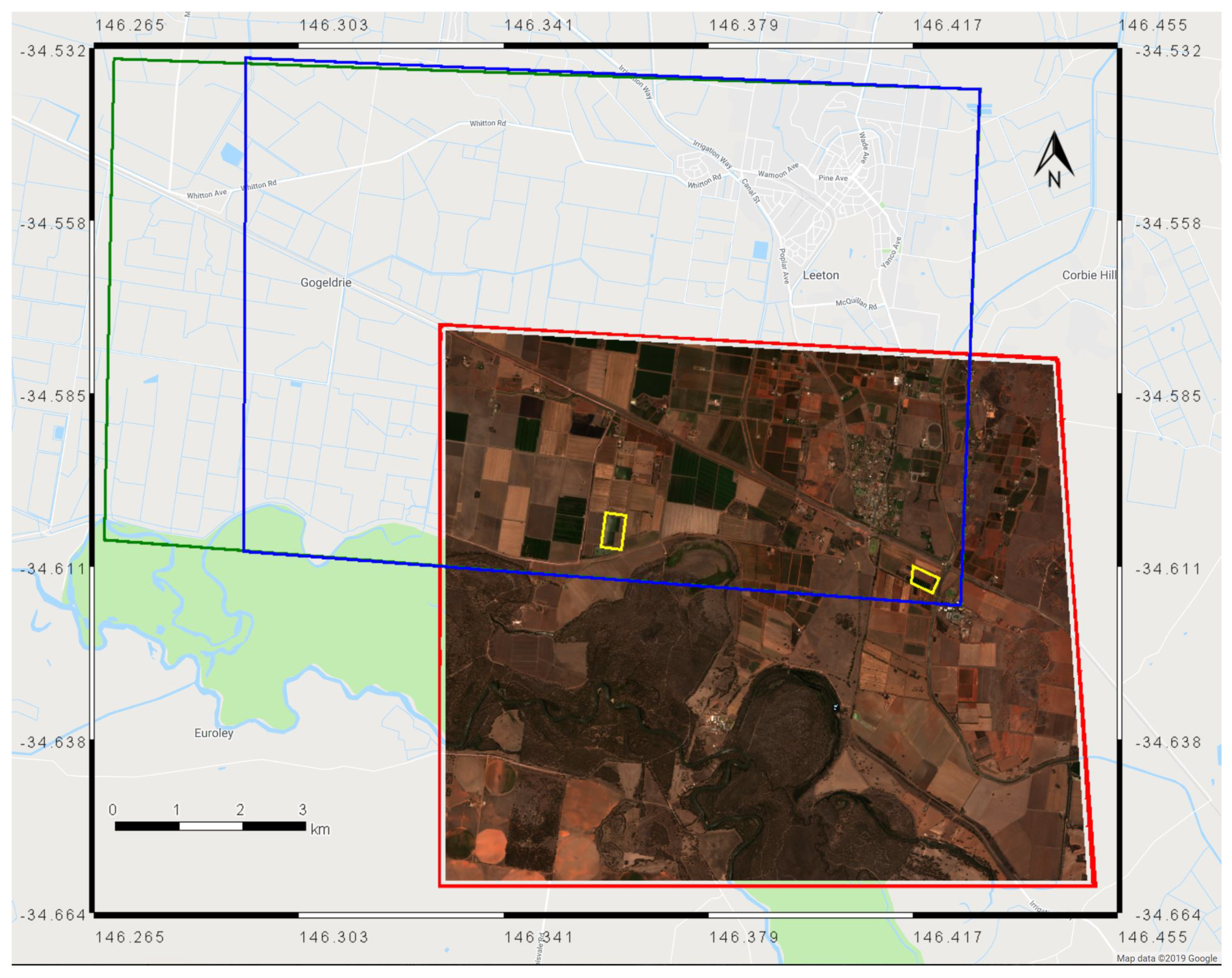
The study was based in Leeton, NSW, Australia. A list of all the experiments used in this work is given in

Table 1. Table of experiments, indicating management dates and N rates, rice varieties and number of plots. For experiments with multiple sowing dates, the early date is denoted SD1 and the later SD2.

Year	Site	Exp	N Rates (kg/ha)	Varieties	Plots	First Flush	Perm Water	Sample	Image
2015	LFS		0, 60, 120, 180, 240	R, S, L, T	80	16 Oct 2014	20 Nov 2014	29 Dec 2014	21 Dec 2014
2015	YAI	SD1	0, 60, 120, 180	R, S, L, T	48	10 Oct 2014	19 Nov 2014	30 Dec 2014	21 Dec 2014
2015	YAI	SD2	0, 60, 120, 180	R, S, L, T	48	27 Oct 2014	27 Nov 2014	5 Jan 2015	21 Dec 2014
2016	LFS	SD1	75, 150, 225, 300	R, S, L, T	48	21 Oct 2015	26 Nov 2015	30 Dec 2015	30 Dec 2015
2016	LFS	SD2	75, 150, 225, 300	R, S, L, T	48	5 Nov 2015	4 Dec 2015	31 Dec 2015	30 Dec 2015
2016	YAI		0, 60, 120, 180, 240	R, S, L, T	60	15 Oct 2015	20 Nov 2015	30 Dec 2015	30 Dec 2015
2017	LFS		0, 60, 120, 180, 240, 300	R, S, L, T	72	31 Oct 2016	2 Dec 2016	6 Jan 2017	7 Jan 2017
2017	YAI		0, 60, 120, 180, 240	R, S, L, T	60	20 Oct 2016	1 Dec 2016	9 Jan 2017	7 Jan 2017
2018	LFS		0, 60, 120, 180, 240, 300	R, L, T	54	30 Oct 2017	30 Nov 2017	6 Jan 2018	9 Jan 2018
2018	YAI		0, 60, 120, 180	R, L, T	36	27 Oct 2017	1 Dec 2017	6 Jan 2018	9 Jan 2018

. It includes data from four rice growing seasons (harvest in autumn each year from 2015–2018), four rice varieties (Reiziq™, Sherpa™, Langi and Topaz™), multiple sowing dates and two sites with differing soil types (Yanco Agriculture Institute (YAI) [146.425E, 34.618S] and Leeton Field Station (LFS) [146.361E, 34.606S]). The soil types of these sites according to the definitions in [42] are red-brown earth at YAI, and self-mulching clay at LFS. Further soil properties at these sites are described in [30]. Sowing date is usually a day before the date of first flush shown in Table 1. One image per season was acquired from the WorldView-2 (2015 and 2016) or WorldView-3 (2017 and 2018) satellites, with image dates close to PI dates. The study area is shown in Figure 1, together with the satellite image capture areas and field sites.

All experiments were drill sown at 0.19 m row spacing and flush irrigated until the 3 to 4 leaf growth stage (see growth stage definitions in [43]). Several nitrogen rates were applied at this stage with urea spread on the dry soil surface prior to the application of permanent water to the experiments. Table 1 shows the WorldView image dates, first flush (FF) date, permanent water (PW) date, and physical sampling dates. It also shows the number of plots, rice varieties (R = Reiziq™, S = Sherpa™, L = Langi, T = Topaz™) and N rates for each experiment. N rates were within the range 0 to 300 kg/ha, with rates per season and experiment indicated in Table 1. There are at least three replicates of each N × variety treatment in each experiment. Plot sizes ranged from 6.3 × 5.7 m${}^2$ to 10.5 × 11.4 m${}^2$. Each plot was sampled on a number of dates, only the sample date closest to the image date is shown in Table 1.

2.2. PI N Sampling Methodology

Panicle initiation (PI) occurs at the start of the reproductive phase in rice growth. There are methods to predict the timing of PI using environmental variables [44]. Field sampling was used to determine the exact time of PI, defined as the time when three out of ten main stems have a panicle 1–3 mm long [14].

Above ground plant samples were collected from each plot at PI from an area of six plant rows (0.19 m row spacing) by one metre. Five whole plant grab samples including leaves and stems (approximately 20 g each) were collected from each sample to create a 100 g subsample which was dried in a microwave oven before being dried overnight in a conventional oven at 60 ${}^{°}$C. This subsample was ground and analysed for N concentration by Dumas combustion [45] and multiplied by the measured dry matter weight to calculate PI nitrogen uptake.

2.3. Climate Data

In order to assess the possibility that climate variation from season-to-season could affect the relationship between rice N uptake at PI and remotely sensed data, weather data for each of the seasons was obtained and processed. Aggregated climate parameters between critical management and measurement days were calculated, these days being the first flush (FF), the date permanent water (PW) was applied, the date the N uptake was sampled and the date the satellite image was captured.

Growth degree days [46] was calculated. The base temperature was set to 10 ${}^{°}$C, which is commonly used in the Australian rice growing system [44]:

$$\mathrm{GDD}=\sum _{t_0}^{t_N}(T_{\max }+T_{\min })/2-10,$$

(1)

where $t_0$ and $t_N$ are the beginning and end days of the GDD summation, and $T_{\max }$ and $T_{\min }$ are the daily maximum and minimum temperatures, respectively.

The sum of solar radiation between dates was calculated by accumulating daily solar radiation. Reference evapotranspiration (ETo) in mm was calculated from weather observations using the standardized ASCE equation [47]. In this work, the sum of these parameters between two dates will be indicated using nomenclature such as GDD(image-FF) for the accumulated growth degree days between the image date and first flush date.

2.4. Worldview Satellite Data

The 21 December 2014 and 30 December 2015 images were from the WorldView-2 satellite, with 2 m resolution for the multispectral bands. The 7 Januar 2017 and 9 January 2018 images were from the WorldView-3 satellite, with 1.2 m multispectral resolution. All imagery was acquired under cloud-free conditions. The band definitions of the sensors on both platforms are shown in

Table 2. WorldView-2 and WorldView-3 band definitions.

Abbreviation	Band	Band Edges (nm)
c	Coastal	400–450
b	Blue	450–510
g	Green	510–580
y	Yellow	585–625
r	Red	630–690
re	Red edge	705–745
nir	Near infrared	770–895
nir2	Near infrared 2	860–1040

.

The satellite images were imported into Google Earth Engine [48] where subsequent image analysis was performed. The at-sensor pixel data were converted to top-of-atmosphere reflectance using the metadata supplied with the images, and the procedure given by the image provider at https://www.digitalglobe.com/resources. Then, atmospheric haze correction was applied using the Dark Object Subtraction method [49].

Shapefiles of each of the trial plots for each season, site and experiment were created and overlaid on the satellite imagery. The averages of each of the eight band reflectances for each plot were calculated (with plot boundaries internally buffered by 1 m to avoid edge effects), and exported as a data table for further analysis.

2.5. Data Pre-Processing

Data analysis was performed using the Python programming language in Google’s Colaboratory cloud-based environment. Extensive use was made of tools such as Pandas [50], and the scikit-learn [51] and StatsModels [52] packages for statistical modeling. Data from the various sources was merged:

• Satellite remote sensed data (average band reflectances per plot).
• Aggregated climate (GDD, Solar, ETo) data and number of days between dates of first flush, permanent water, sample collection, image capture.
• Field rice sample data (N uptake per plot). For most experiments in Table 1, the plots were sampled numerous times to correspond with dates of image capture and growth stage. So the dataset had a row for each of these samples (i.e., multiple rows per plot).

As well as the raw reflectances, ratio and normalized difference indexes were calculated. It is commonly understood that taking ratios of remotely-sensed reflectances provides some normalization against the effects of variable radiance and atmospheric absorption between image captures. Therefore, as well as investigating the relationship between the band reflectances and N uptake, 2-band ratio spectral indexes (RSIs) and normalized difference spectral indexes (NDSI) from the 8 reflectance bands were investigated, defined as [28]:

$$\begin{array}{cc}\hfill \mathrm{RSI}(b1,b2)& =b1/b2\hfill \end{array}$$

(2)

$$\begin{array}{cc}\hfill \mathrm{NDSI}(b1,b2)& =(b1-b2)/(b1+b2)\hfill \end{array}$$

(3)

For example, the widely used normalized difference vegetation index (NDVI) is NDSI(nir,r), and the normalized difference red edge (NDRE) is NDSI(nir,re). All possible RSIs and NDSIs from all independent combinations of the eight reflectance bands in Table 2 were calculated and added to the dataset.

A number of additional vegetation indexes that aren’t RSIs or NDSIs were also trialled. These were shown to be significant for predicting N uptake in previous works [25,28]:

$$\begin{array}{cc}\hfill \mathrm{CIre}& =nir/re-1\hfill \end{array}$$

(4)

$$\begin{array}{cc}\hfill \mathrm{CIg}& =nir/g-1\hfill \end{array}$$

(5)

$$\begin{array}{cc}\hfill \mathrm{SAVI}(\mathrm{nir},\mathrm{re})& =(1-0.08)\times (nir-re)/(nir+re-0.08)\hfill \end{array}$$

(6)

2.6. N Uptake Models

2.6.1. Single-Variable Models

Data from all the experiments was pooled. As the N uptake was sampled on multiple dates for each experiment, data from the sample dates closest to the image dates was chosen for preliminary analyses, which are the sample dates shown in Table 1.

Correlation analysis was performed of all RSI and NDSI bands against N uptake, to determine which are likely to be the dominant predictors. This indicates how well a linear model can describe the relationship between N uptake and spectral indexes:

$$y=a\times x+b$$

(7)

where a and b are the slope and intercept of the model, y is N uptake and x is the spectral index being assessed. This nomenclature is used throughout this paper. The coefficient of determination R${}^2$ was used to quantify the power of each index to explain the variance in the N uptake:

$${\mathrm{R}}^2=1-\frac{{\sum }_{i=0}^{N-1}{(y_i-{\widehat{y}}_i)}^2}{{\sum }_{i=0}^{N-1}{(y_i-\overline{y})}^2}$$

(8)

where N is the number of observations, ${\widehat{y}}_i$ is the i-th model prediction and $y_i$ is the i-th observation, and $\overline{y}$ is the mean of the observations.

Models were further evaluated using the root mean squared error (RMSE):

$$\mathrm{RMSE}=\sqrt{\sum _{i=0}^{N-1}{(y_i-{\widehat{y}}_i)}^2/N}$$

(9)

RMSE is an easily interpretable measure of model performance as it retains the units of the quantity being observed and predicted. In our case, this is kg/ha of N uptake. Note, in other studies, N uptake or plant nitrogen accumulation (PNA) is reported in g/m${}^2$, which can be converted to N uptake in kg/ha by multiplying by ten.

Model coefficients were tested for significance at the p = 0.05 level using the StatsModels Ordinary Least Squares methods (statsmodels.regression.linear_model.OLS).

Following this, nonlinear transformations were investigated to enable models to better fit N uptake. These included the exponential transformation:

$$\begin{array}{cc}\hfill y& =b{\exp }^{a\times x}\hfill \end{array}$$

(10)

$$\begin{array}{cc}\hfill \ln y& =a\times x+\ln b\hfill \end{array}$$

(11)

where a and b are the regression coefficients. N uptake is denoted by y in this and following equations, and x is the vegetation index being used (for example, NDRE). The second line indicates that by taking the logarithm of both sides of the equation, the model can be fit using linear regression. The disadvantage of this formulation is that the predicted variable, $\ln y$, no longer has units of kg/ha.

A second transformation involved squaring the unitless input vegetation index. It will be shown that this linearizes the N uptake vs. index relationship, when the selected index is NDRE, and also renders the y-intercept insignificant. This squared transformation is:

$$y=a\times x^2+b\approx a\times x^2$$

(12)

where a is the slope of the N uptake vs. $x^2$ line, and b is the intercept.

In order to assess the effect of secondary factors (such as season, variety, site, sowing date) on the models, Equation (12) was fit to subsets of the data. The regression lines for each subset were assessed for significant difference from the regression line of the whole dataset by first dividing the N uptake by $a\times {\mathrm{NDRE}}^2$ (with a set to the extracted coefficient for the whole dataset), then applying the Tukey HSD test at the alpha = 0.05 level (using the statsmodels.stats.multicomp.pairwise_tukeyhsd component of the StatsModels package in Python [52]).

2.6.2. Multi-Variable Models

The analysis then proceeds to multi-variable linear regression, to investigate how much more accurate the N uptake model can be across seasons, varieties, sites, management with more complex models. The possible inputs to the model are: reflectances, RSIs, NDSIs, varieties, all combinations of dates between [first flush, permanent water, image, sample], as well as the growth degree days, solar radiation, rain and evapotranspiration over these days.

Relationships between N uptake and input variables often followed a squared rather than linear trend. In addition, interaction between many of the input variables was found to be significant, as evidenced by variable selection methods (described below) making use of these interaction terms. Therefore, the input variables were transformed with a second-order polynomial so that squared terms of all input variables, and cross terms between all combinations of input variables were generated. As a simple example, if the raw input variables were [NDRE, NDVI], the transformed variables would be [NDRE${}^2$, NDRE × NDVI, NDVI${}^2$]. In practice, we considered models with up to 33 variables (including remotely sensed bands, variety, climate parameters, important dates), giving 594 transformed variables. The input variables were then scaled using the standard scaler in scikit-learn (sklearn.preprocessing.StandardScaler). This centers and normalizes the variances of each of the input variable data, which is important for fitting models with regularization (described below).

In order to produce models that are interpretable and straightforward to implement in a variety of GIS platforms, black-box models such as SVM models and neural networks were avoided. Instead, we used linear regression with Lasso regularization from the scikit-learn package (sklearn.linear_model.Lasso). This has the advantage of selecting the most important input variables and setting all others to 0, because it uses L1 regularization [53]. The Lasso objective is to minimize the following, with $w_j$ being the coefficient of each input variable $x_j$ and ${}_i$ denoting observation number:

$$\sum _i{(y_i-\sum _j{x}_{ij}{w}_j)}^2+\alpha \sum _j\left|w_j\right|$$

(13)

The Lasso $\alpha$ parameter multiplies the L1 term, so larger values of $\alpha$ result in more compact models (more coefficients $w_j$ set to 0). The relative importance of the input variables can be assessed by examining the magnitude of the remaining coefficients.

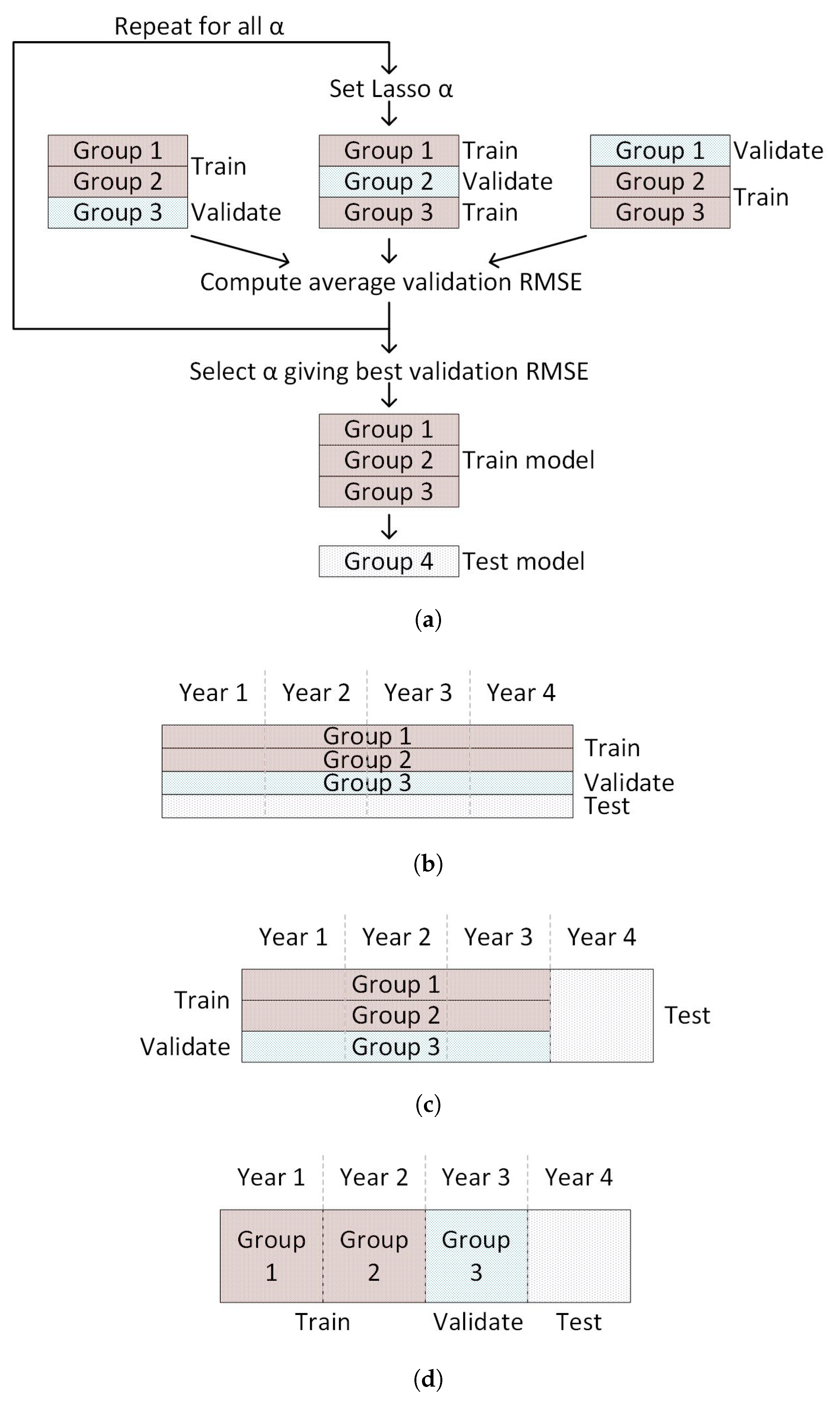
Three-fold cross validation was used to select the best Lasso $\alpha$ using the GridSearchCV tool in scikit-learn (sklearn.model_selection.GridSearchCV [51]). This splits the training/validation data into three groups, training a model on two and validating (assessing the accuracy of model predictions using a score such as RMSE) on the third. The procedure is illustrated in Figure 2a. This is done three times, first with groups 1 & 2 as training data and group 3 as validation data, then groups 1 & 3 as training data and group 2 as validation data, then groups 2 & 3 as training data and group 1 as validation data. The average of the validation scores (RMSE of N uptake prediction) is taken. This process is repeated as the Lasso $\alpha$ was swept. The $\alpha$ that gives the best average RMSE score is selected. The model is then re-trained with this best $\alpha$ with all the training/validation data. Finally, this model was evaluated on it’s ability to predict the held back test data.

2.6.3. Multi-Season Models

Three ways of splitting the multi-season data into training, validation and test sets were evaluated. The first is shown in Figure 2b. The entire data set was split randomly into training/validation and test data, with 30 % of the data held for test.

However, for operational use, models need to be trained on previous season data to predict N uptake at PI for a new season, so that topdressing can be applied soon after an image is captured. To assess the ability of the remotely sensed data to achieve this aim, a second method of splitting data took the training data from three seasons and the extracted model was tested on the fourth season data, as shown in Figure 2c. Three-fold cross validation was used with Lasso regression to select the best $\alpha$, with randomly selected training and validation points from three season’s data. Then this model’s prediction was tested on the remaining season’s data. The WorldView 8-band reflectances were used as the input variables, with the NDRE${}^2$ band added, which was found to increase accuracy. It will be shown that this method overfits the model to the three training seasons, and so does not generalize well to the fourth test season.

To seek to solve this overfitting issue, a different cross-validation method was used to select the optimal Lasso $\alpha$ from the three training seasons, shown in Figure 2d. Rather than randomly assigning points from the three training seasons to model training and validation sets over three folds, the training and validation sets included two seasons and one season respectively. This was implemented using the Leave One Group Out method in scikit-learn (sklearn.model_selection.LeaveOneGroupOut) [51]. For example, for testing the model on the 2018 season, the cross validation for Lasso model training used [training, validation] folds of [2015 + 2016, 2017], [2015 + 2017, 2016], [2016 + 2017, 2015] to select $\alpha$, before testing the final model on the 2018 data. Because the model training process is validating performance against a held out season data in each of the cross validation folds, the model can then generalize better to a totally new season, as overfitting to within-season data is avoided.

3. Results

3.1. Correlation between Remotely Sensed Data and N Uptake

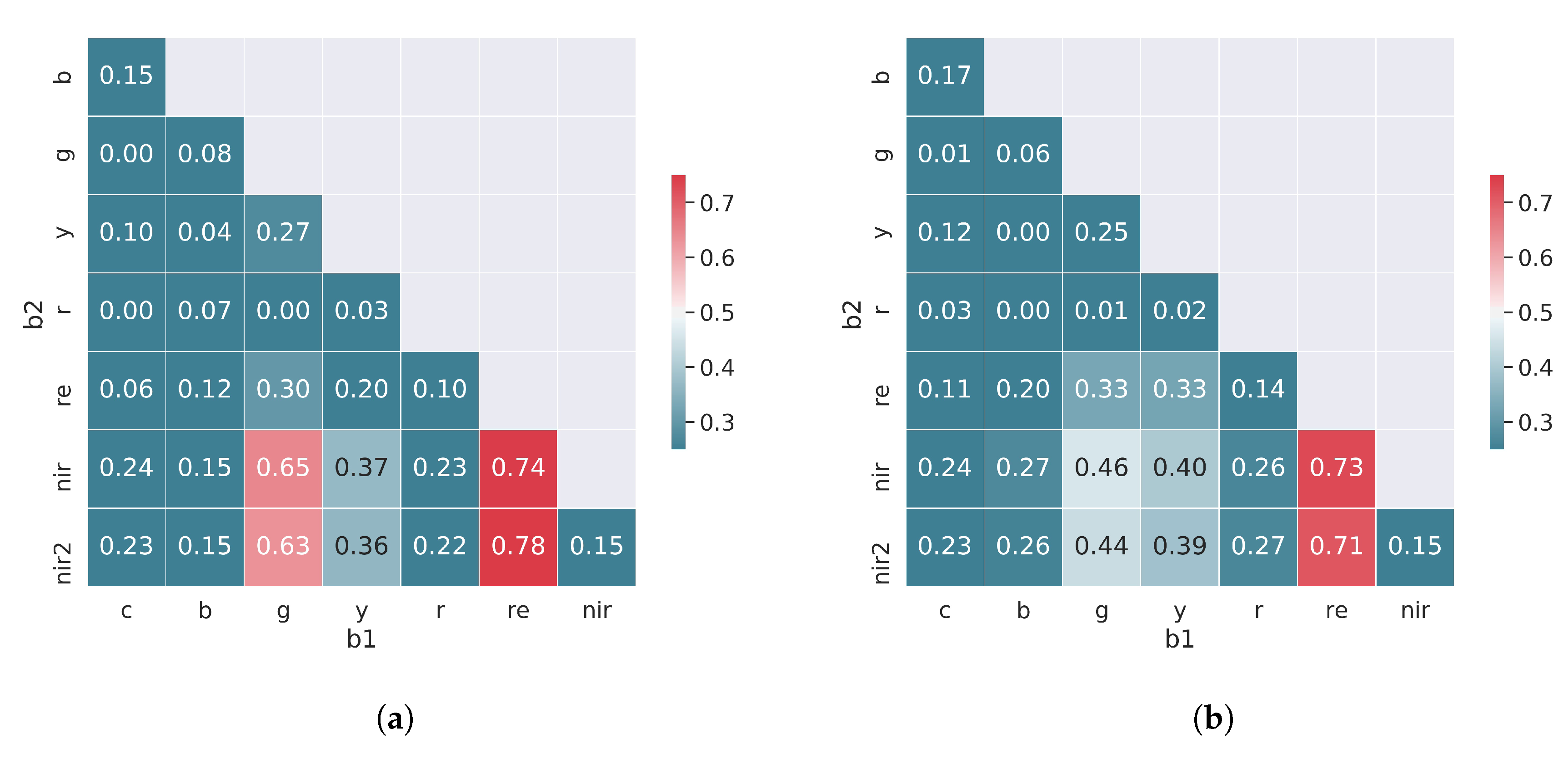
The correlation between each of the RSIs and NDSIs and N uptake for the pooled data from all experiments was assessed using the coefficient of determination (R${}^2$). The results are shown in Figure 3. The best ratio index is RSI(nir2,re) with R${}^2=0.78$, closely followed by RSI(nir,re) with R${}^2=0.74$. For the normalized difference indexes, the best index is NDRE = NDSI(nir,re), with R${}^2=0.73$. These results indicate ratio indexes are at least as good as normalized difference indexes for predicting N uptake. The single-variable linear regression analysis that follows uses NDRE as the input variable. The performance using other combinations of bands will be described in following sections.

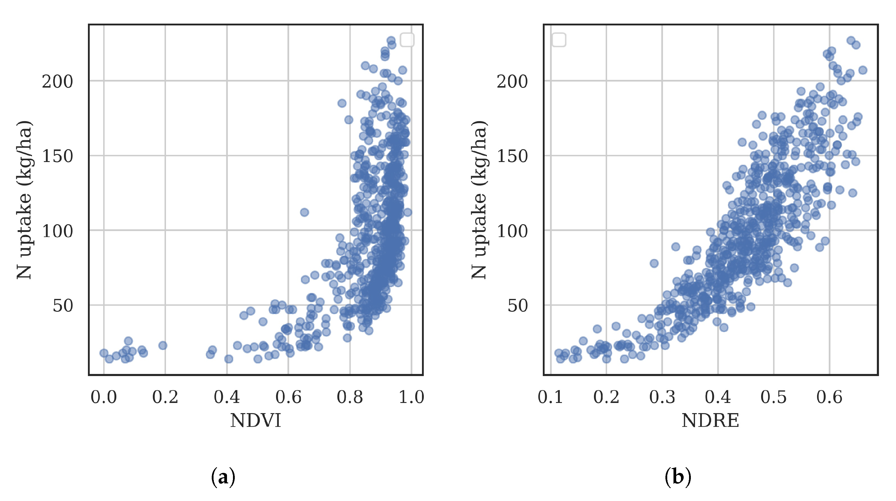
NDVI (R${}^2$ = 0.26) does not perform as well as NDRE (R${}^2$ = 0.73), as seen in Figure 3. The reason for this is indicated in Figure 4. NDVI saturates at large values of N uptake. In contrast, NDRE continues to increase at high values of N uptake, making it a better predictor.

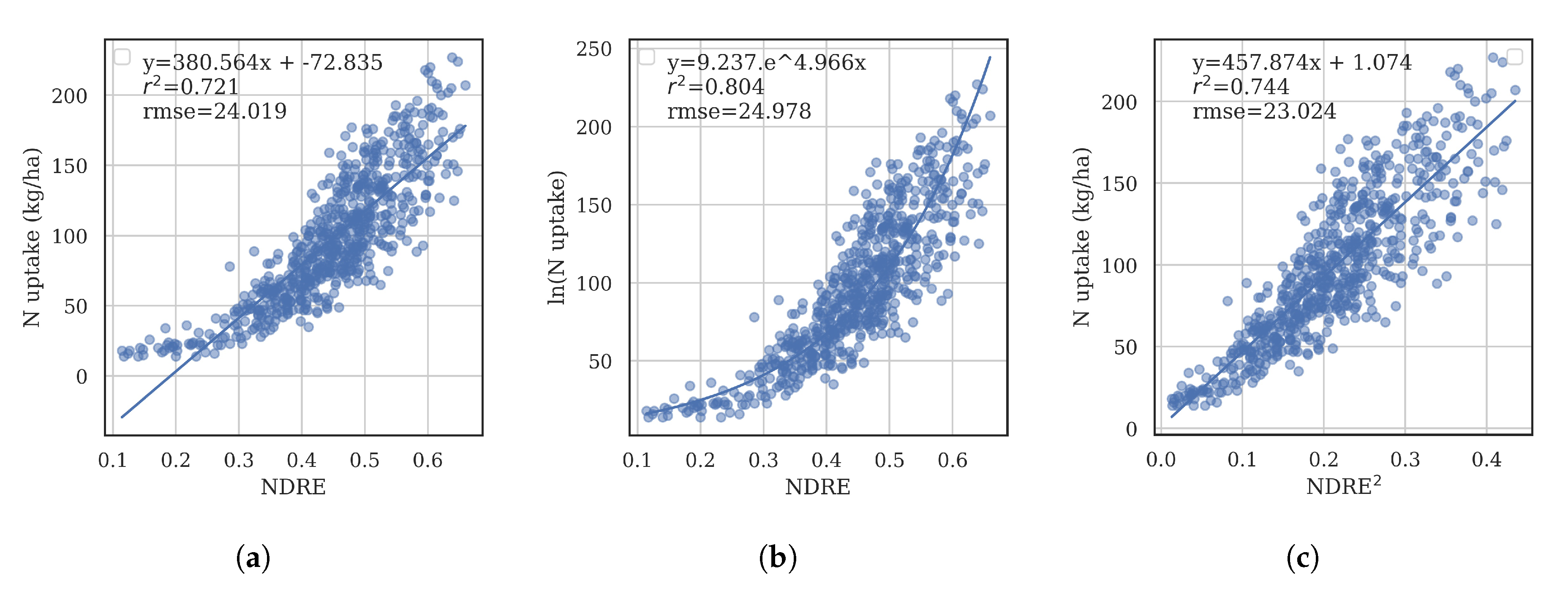
There is a nonlinear relationship between NDRE and N uptake, evident in Figure 4b. Fitting a linear model leads to large residuals at high and low values of N uptake. Various equations were used to attempt to capture this relationship. Two are shown in Figure 5. An exponential relationship appears to fit the trend of the data closely, as seen in Figure 5b. This is described by Equation (10). The disadvantage of this formulation is that the predicted variable (logarithm of N uptake) no longer has units of kg/ha, making evaluation statistics such as RMSE difficult to interpret.

Another possibility to describe the nonlinear relationship between NDRE and N uptake is shown in Figure 5c, where instead of transforming the predicted variable (N uptake), we square the unitless input variable NDRE. This model is described by Equation (12). This transformation linearizes the N uptake vs. index relationship. It also gives a lower RMSE than the linear or ln(N) options and the predicted variable retains physical units of kg/ha.

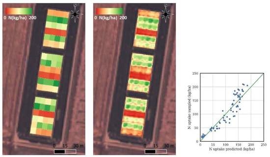
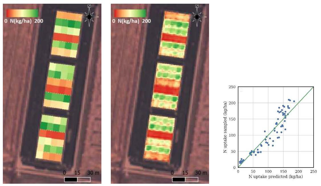
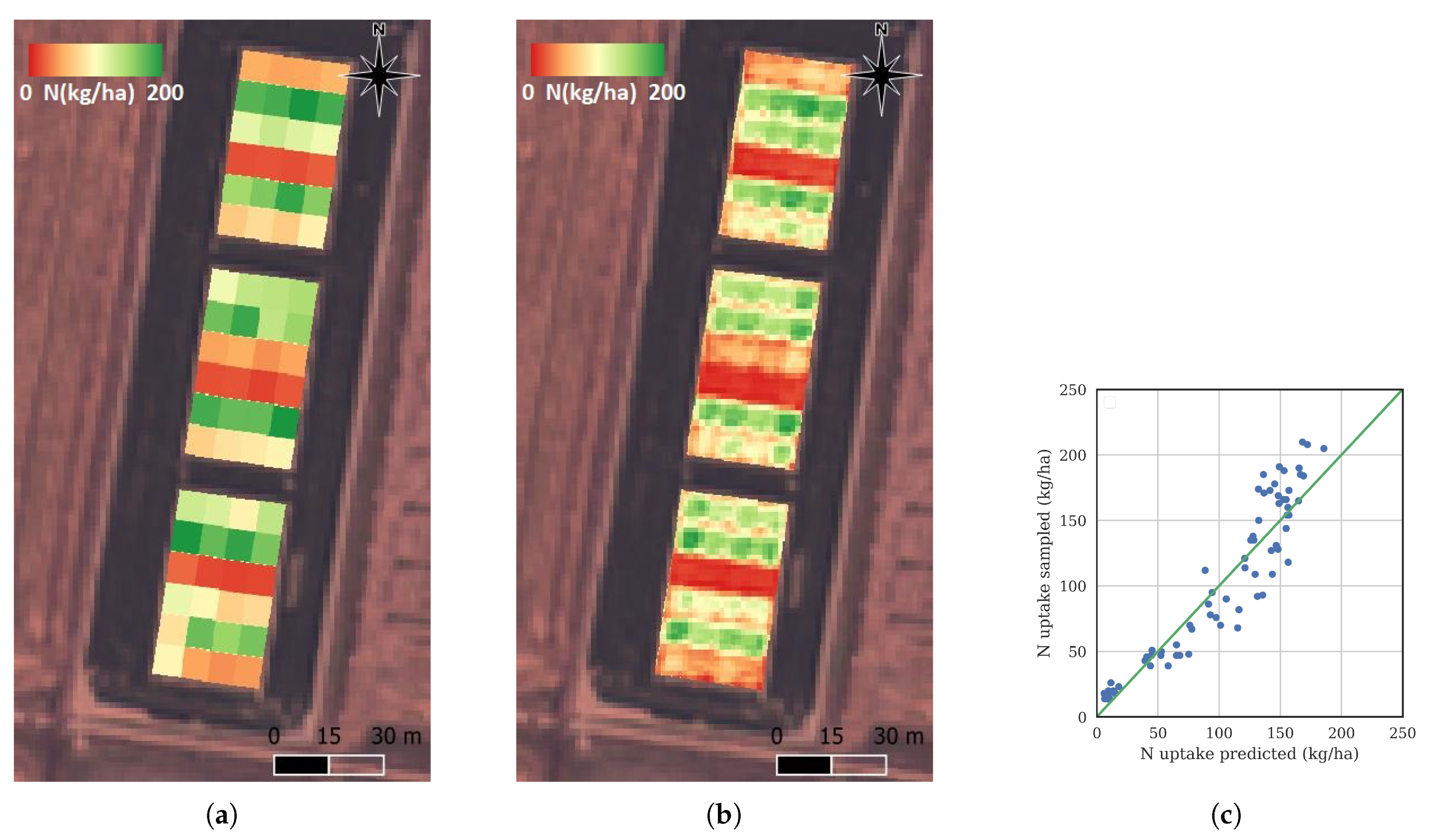
The y-intercept of the N uptake vs. NDRE${}^2$ model was not significant at p < 0.05, so was omitted. The slope was significant at p < 0.05. The resulting model equation fit to the four-season dataset is $y=a\times x^2=457\times {\mathrm{NDRE}}^2$. The residuals were examined and followed a normal distribution. Maps of modeled N uptake were generated using this equation and NDRE computed from the satellite images. Figure 6 shows the measured and predicted N uptake map from the 2017 season at the LFS site. Good agreement is observed, with R${}^2$ = 0.88 and RMSE = 21.3 kg/ha.

3.2. Effect of Secondary Variables On Models

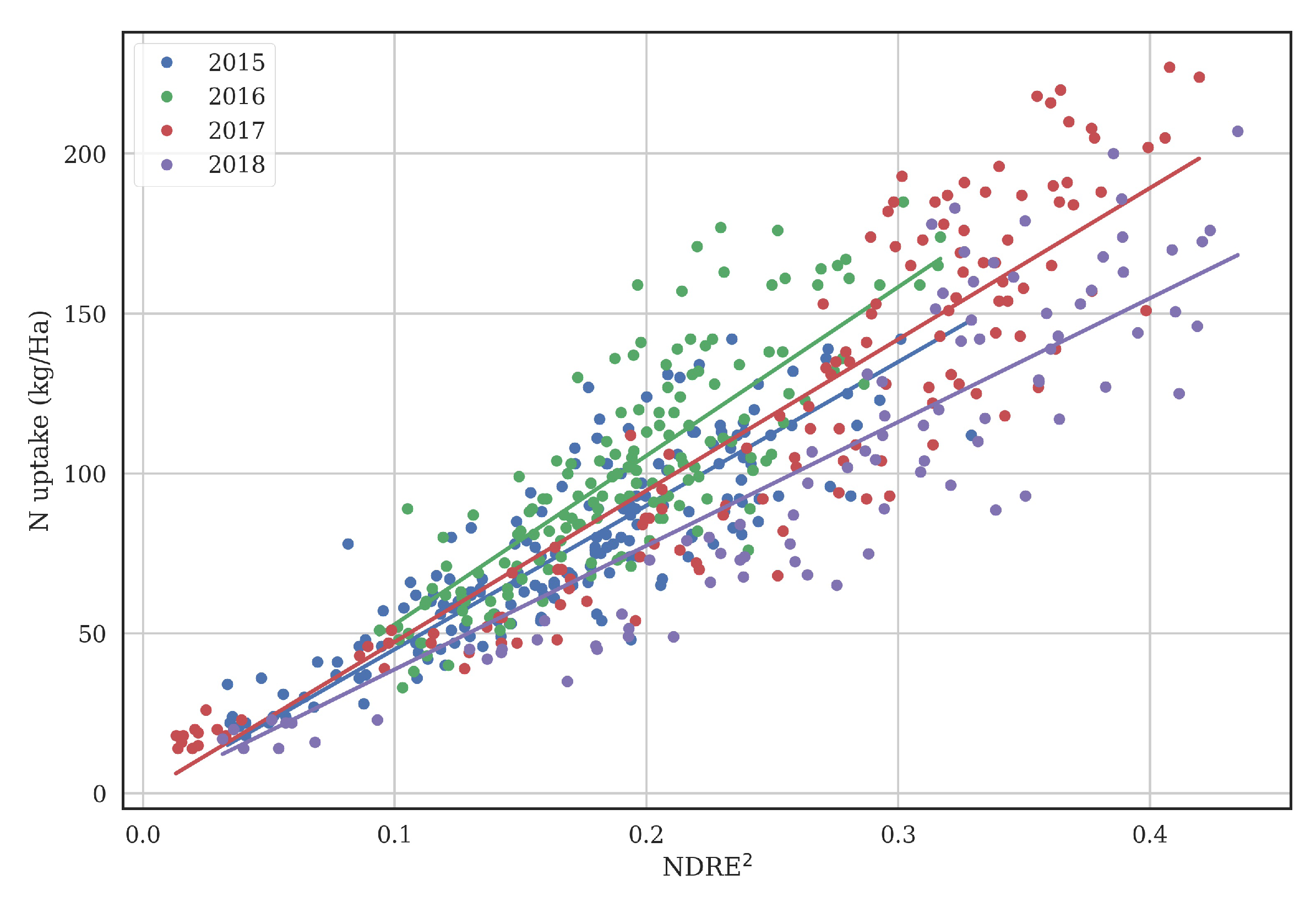
The dataset was split into batches, based on (i) year, (ii) variety, (iii) site and (iv) sowing date; in order to assess the effect of these factors on the relationship between remotely sensed data and N uptake. Equation (12) was fit to each of the subsets of data. The results are shown in

Table 3. Linear regression results for N uptake vs. NDRE${}^2$, with separate regression coefficients for different groupings of experiments.

Variable	Value	Points	a	R${}^2$	RMSE (kg/ha)	Group
ALL	ALL	554	457	0.75	22.8
Year	2015	176	450	0.71	15.5	b
	2016	156	528	0.69	19.2	c
	2017	132	473	0.85	23.1	bc
	2018	90	387	0.80	22.7	a
Variety	Sherpa™	116	491	0.81	19.5	b
	Reiziq™	146	409	0.76	22.9	a
	Langi	146	464	0.79	21.2	b
	Topaz™	146	499	0.79	20.5	b
Site	LFS	302	452	0.83	20.0	a
	YAI	252	463	0.61	25.6	a
Sow date	Early	296	485	0.77	21.0	a
	Late	258	431	0.77	22.9	a

. The statistically significant differences in the subsets are indicated in the Group column of the table. There are significant differences in the model slopes (a) between different years, from 387 (2018) to 528 (2016). The regressions per year are shown in Figure 7. There are significant differences between the Reiziq™model and the other variety models. There are no significant differences between sites or sowing time (before or after 25-October).

3.3. Effect of Different Sampling and Image Dates

There were multiple sample dates for each of the experiments (see Section 2.5), though the analysis up until now has only made use of the sample data closest to the date where the satellite image was captured. Nitrogen uptake is dynamic, so it is reasonable to expect the actual N uptake at the image date will be different to the sampled N uptake if the sample was taken on a different date. To test the effect of different sampling and image dates, sample data from all dates was used, and the data was separated into buckets of 10 days between image and sample date. The model of Equation (12) was fit to each bucket. The results are shown in

Table 4. Linear regression results for N uptake vs. NDRE${}^2$, with separate regression coefficients for different number of days between N uptake sampling and image capture, binned into 10 day buckets.

Days (Image-Sample)	Points	a	R${}^2$
−30	176	586	0.59
−20	48	492	0.27
−10	284	534	0.64
0	600	451	0.76
10	36	336	0.63

. As expected, generally when the N uptake was sampled after the image capture (negative Days(image-sample)), the regression slope is steep, as the N uptake would have increased relative to NDRE${}^2$. The best relationship is observed when the sampling date is close to the image date, as indicated by the highest R${}^2$ = 0.76 with Days(image-sample) = 0.

3.4. Improving the Accuracy of The Model

Up until now, a single input variable model has been used (Equation (12) with $x=$ NDRE). In this section, more complex multi-variable linear regression models are explored, using Lasso regression to avoid overfitting and to eliminate insignificant variables, as described in Section 2.6.2.

First, data for training/validating and testing the models are randomly chosen from all four seasons, as shown in Figure 2b. The results are shown in

Table 5. Results from multi-variable regression models with all season data pooled, and train/test points randomly selected (as shown in Figure 2b). #X is the number of raw input variables. #(X)${}^2$ is the number of input variables after the polynomial is applied. # selected X is the number of variables selected after Lasso regularization. Most important X shows the three most important variables.

Input Variables	Best $\mathit{\alpha }$	# X	# (X)${}^2$	# Selected X	Train R${}^2$	Test R${}^2$	Train RMSE	Test RMSE	Three Most Important X
NDVI	0	1	1	1	0.24	0.30	38.1	41.4	NDVI
NDRE	0	1	1	1	0.72	0.74	23.2	25.5	NDRE
NDRE${}^2$	0	1	1	1	0.74	0.77	22.3	23.7	NDRE${}^2$
CIre	0	1	1	1	0.73	0.77	22.8	23.8	CIre
CIg	0	1	1	1	0.63	0.67	26.7	28.5	CIg
SAVI	0	1	1	1	0.62	0.67	26.9	28.5	SAVI(nir,re)
RSI4	0.01	6	27	19	0.83	0.82	18.2	20.8	RSI(r,g) × RSI(re,g), RSI(r,g), RSI(re,g)
RSI8	0.1	28	434	24	0.86	0.85	16.2	19.5	RSI(nir2,re) × RSI(nir2,nir),
									RSI(b,c) × RSI(re,r), RSI(nir2,c) × RSI(nir2,re)
NDSI4	0.04	6	27	10	0.82	0.82	18.4	21.0	NDSI(nir,re)${}^2$, NDSI(r,g) × NDSI(re,g),
									NDSI(r,g)${}^2$
NDSI8	0.1	28	434	21	0.86	0.85	16.2	18.9	NDSI(nir2,re)${}^2$, NDSI(re,c)${}^2$,
									NDSI(y,c) × NDSI(r,b)
R4	0.004	4	14	13	0.87	0.87	15.7	17.7	nir${}^2$, re × nir, r × re
R8	0.004	8	44	29	0.90	0.90	13.9	16.0	b × r, c × b, c${}^2$
R8 × variety	0.02	12	90	36	0.91	0.89	13.3	16.2	nir2${}^2$, g × re, g × nir
R8 × climate	0.02	29	464	39	0.92	0.91	12.7	14.6	nir2${}^2$, re × nir, nir × Rain(image-PW)
R8 × variety × climate	0.020	33	594	61	0.93	0.91	11.7	14.9	re × r, nir × Sow_week, nir × Rain(image-PW)
As above, all sample dates	0.004	33	594	110	0.93	0.90	12.4	14.2	y × Sow_week, nir × Solar(image-PW), g × re

. Models with different numbers and combinations of input variables were tested. Many multispectral sensors have less bands than the 8 bands of the WorldView sensors (Table 2). Therefore, models were generated using only 4 out of the 8 possible bands to test degradation in accuracy expected with less capable sensors. These four bands are g, r, re, nir.

The first group of models at the top of Table 5 shows results from single input variable models (Lasso $\alpha$ = 0 as no variable selection is needed). The second group of models in the middle of the table includes all RSIs and NDSIs formed by combinations of all reflectance bands. Results are shown for all combinations of 4 bands b, g, r and nir (RSI4 and NDSI4), as well as all combinations of WorldView sensor’s 8 bands (RSI8 and NDSI8). The third group of models are for combinations of the raw reflectance bands without taking ratios or normalized differences (R4 and R8). The final models also add variety and climate data. The model in the last row adds in all sample data, with multiple sample dates per image capture (see Section 2.5).

For each combination of input variables, the table indicates the best Lasso $\alpha$, which gave the lowest validation RMSE. It also shows the number of raw input variables (# X), the total number of input variables after processing with a second-order polynomial (# (X)${}^2$), and the number of variables that were retained after Lasso regularization (# selected X). The last column in the table shows the 3 most significant input variables used in the model.

For the single-input variable models, NDRE${}^2$ is the best predictor of N uptake, with test RMSE of 23.7 kg/ha.

Models using combinations of RSIs and NDSIs achieve similar performance, with 8 bands improving RMSE by 1–2 kg/ha relative to 4 bands. NDSIs using 8 bands yielded N uptake RMSE of 18.9 kg/ha.

Using the raw reflectances (R4 and R8 in the third section of Table 5) instead of RSIs or NDSIs yields lower errors by around 3 kg/ha. Adding variety data does not improve the model. Adding climate and management date variables (R8 × climate) does improve the model by around 1.5 kg/ha to 14.6 kg/ha. The most important bands in the models are re, nir and nir2.

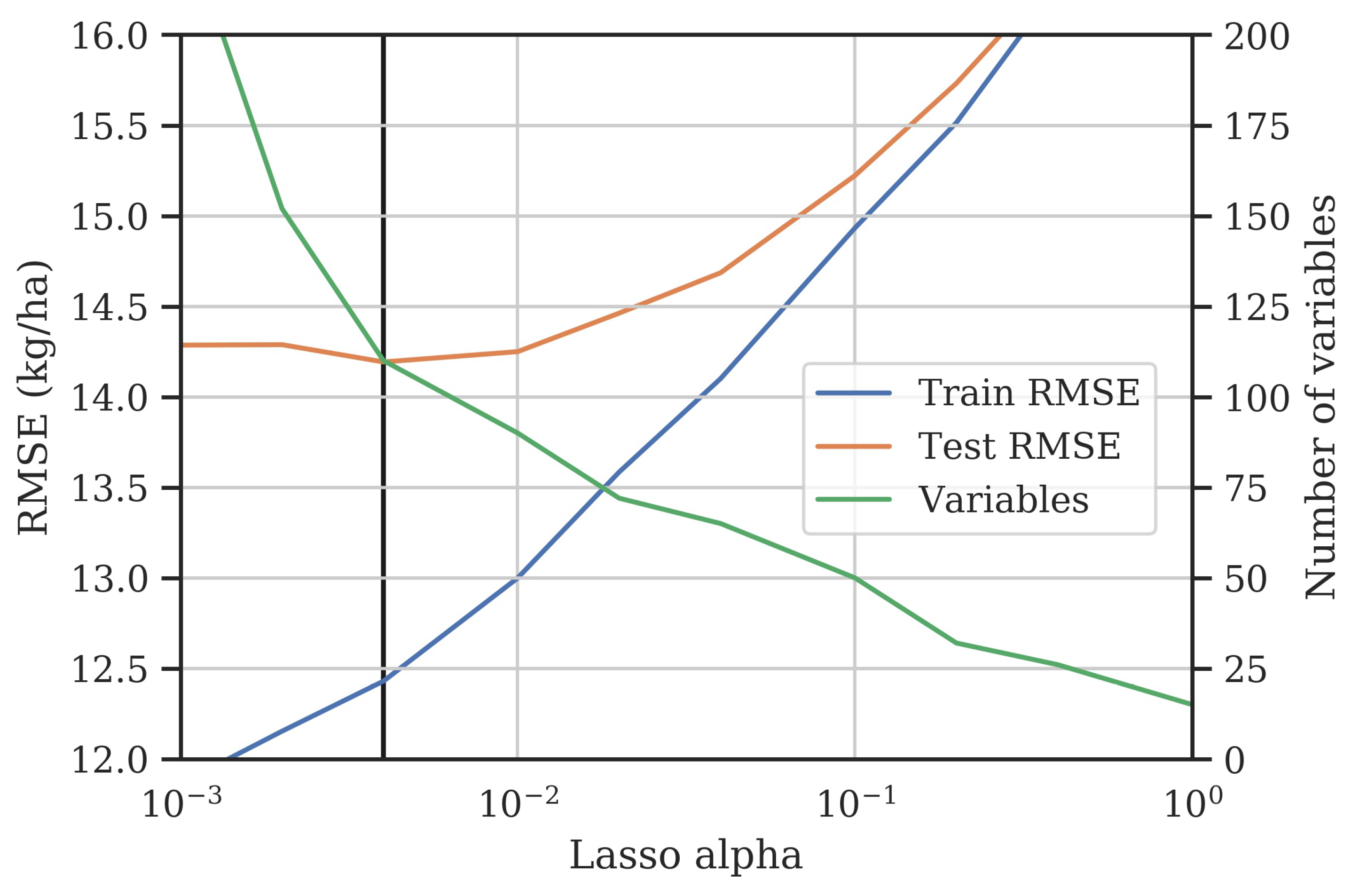
The final row in Table 5 shows the results from the model extracted using N uptake data from all sample dates. The Lasso regularization selected 110 input variables and achieved an R${}^2$ of 0.90 and RMSE of 14.2 kg/ha on the test data. An example of the training and test RMSE and the number of selected model features as a function of the Lasso alpha is shown in Figure 8, corresponding to this last row in Table 5. The figure demonstrates that reducing alpha increases the number of input variables, which gives lower RMSE on the training data, but results in overfitting so that RMSE on the test data is degraded. The optimum alpha is chosen as the one giving the lowest test RMSE, in this case, 0.004. This model is significantly better than the simple single input variable models. However, the model becomes difficult to interpret because of the large number of input variables. It is also questionable if the model will fit future season’s data accurately, a consideration that will be explored in the following section.

3.5. Model Consistency with Season

Previous sections have pooled data from all seasons, with models trained on randomly selected training and test data points from the pooled data. It was seen that using this method, where model training data includes points from seasons being predicted, quite good absolute accuracy can be achieved (RMSE < 20 kg/ha). Now we examine the ability of models trained on three known seasons to predict results in a fourth unknown season, using the methods described in Section 2.6.3.

The first method randomly selects training and validation data from three seasons, then tests on the fourth, as shown in Figure 2c. The results are shown in

Table 6. Lasso regression with one year held out as test data, and the other three years as training data with randomized cross validation (as shown in Figure 2c).

Test Year	Best $\mathit{\alpha }$	# X	# (X)${}^2$	# Selected X	Train R${}^2$	Test R${}^2$	Train RMSE	Test RMSE
2015	0.002	9	54	43	0.93	0.65	13.2	17.2
2016	0.001	9	54	53	0.92	0.38	13.5	27.2
2017	0.001	9	54	48	0.89	−27.04	12.6	311.1
2018	0.004	9	54	29	0.91	−6.47	13.5	140.4

. The models use the eight raw bands and NDRE${}^2$ as input variables. All combinations of training/validation and test years are evaluated. The resulting models are quite complex with small $\alpha$ and more than 29 input variables selected. When the model is trained on 2016–2018 data, and tested on the 2015 data, reasonable performance is achieved (RMSE = 17.2 kg/ha). However, for other test seasons, the predictions are poor. The models with 2017 and 2018 test seasons give a negative R${}^2$. This is possible with R${}^2$ defined as in Equation (8), and indicates the models are not generalizing to the test data. These results indicate that when models are tested on data from unseen seasons using the model training methodology in Figure 2c, generated models may overfit the training/validation data and so will be unlikely to predict future season N uptake accurately.

To seek to solve this overfitting issue, a different cross-validation method was used to select optimal Lasso $\alpha$. This is shown in Figure 2d, and proceeds by holding out one of the training seasons for model validation, and repeating over three combinations of training/validation seasons in three-fold cross validation, before testing on the remaining season from which the model has not seen data. The results using this method are shown in

Table 7. Lasso regression with one year held out as test data, and the other three years as training data with cross validation splits based on training data years (as shown in Figure 2d).

Test Year	Best $\mathit{\alpha }$	# X	# (X)${}^2$	# Selected X	Train R${}^2$	Test R${}^2$	Train RMSE	Test RMSE	Three Most Important X
2015	10.0	9	54	3	0.79	0.67	22.5	16.8	nir2 × NDRE${}^2$, nir2${}^2$, g
2016	4.0	9	54	4	0.85	0.67	19.0	19.9	nir2 × NDRE${}^2$, r × NDRE${}^2$, c × re
2017	4.0	9	54	4	0.80	0.78	17.2	27.4	nir2 × NDRE${}^2$, nir2${}^2$, g
2018	4.0	9	54	3	0.84	0.72	17.5	27.4	nir2 × NDRE${}^2$, NDRE${}^2$, g

. Now Lasso regularization has selected quite simple models, with relatively high $\alpha$ and only three or four input variables selected. The worst RMSE across the four test seasons is 27.4 kg/ha, and worst R${}^2$ is 0.67. In all seasons the most important input variable is nir2 × NDRE${}^2$ with strong similarity between models from all four groups of seasons.

In order to assess the simple NDRE${}^2$ model of Equation (12) using this same multi-season model training strategy (Figure 2d), this model was fit to three years data, then tested against the remaining year. The worst case RMSE was 36.0 kg/ha for the 2018 test year. Thus, we confirm Lasso regression with multiple input variables produces better models (worst case RMSE 27.4 kg/ha for the 2018 test year).

4. Discussion

This study has demonstrated the accuracies that can be obtained using multi-spectral satellite data to predict the N uptake of rice at panicle initiation. This is an essential pre-requisite to developing an operational mid-season N topdressing recommendation tool for the rice industry, based on remote sensing.

Table 8. Published research investigating prediction of N uptake of rice. Root mean squared error (RMSE) of the N uptake is given for cases when training and test data come from the same season, and when the test data comes from a different season (worst case is shown). T = tillering, PI = panicle initiation, H = heading, F = filling, MS = multispectral, HS = hyperspectral, PLSR = partial least squares regression, IPLSR = interval PLSR, MLR = multiple linear regression, VI = vegetation index.

Ref	Stage	Platform	Sensor	Model	Seasons	RMSE (kg/ha) Same Seasons	RMSE (kg/ha) Test Season
[54]	T, PI, H, F	Handheld	MS	VI	2	7.07	-
[28]	PI	Handheld	HS	IPLSR	4	11.7	-
[30]	PI	Handheld	HS	PLSR	3	17.4	34.9
[27]	PI	UAV	MS	VI	2	11.5	-
[29]	H	Airborne	HS	PLSR, MLR	3	11.98	67.1
This	PI	Satellite	MS	MLR	4	14.6	27.4

gives a summary of results from a selection of papers on predicting rice N uptake using remote sensing, for papers that report predicted N uptake root mean squared error (RMSE). The table assumes N uptake at jointing is similar to that at PI, and it shows the results for the best model formulation. The last column shows the worst case test season RMSE for the limited number of studies that test models on different seasons than those used to train the models.

Our work indicates that the model generation strategy critically depends on whether in-season sampling data is available. Complex multi-variable models predicting N uptake from remotely sensed data can be very accurate, providing in-season physical samples and remote sensing data is available for the season being predicted. In this case, previous studies have shown N uptake prediction errors as low as 7 kg/ha [54], and many others around 12 kg/ha [27,28,29]. However, these don’t consider the practically important application of predicting N uptake in new seasons for which sampling data is not yet available. With this limitation, we found N uptake RMSEs of better than 19 kg/ha with remote sensing data from four seasons as shown in Table 5. Addition of management and climate data enabled prediction RMSE better than 15 kg/ha.

However, it is rarely the case that in-season data is available by the time predicted N uptake is needed to generate topdressing requirements, a factor which isn’t considered in most previous studies. The timing and logistics from image acquisition with simultaneous physical N uptake sampling, to model extraction from this data, to N uptake prediction, to N recommendation and finally to applying the top-dressing necessitates applying models extracted from previous data to new seasons. However, seasonal variability in models leading to inaccuracy in extrapolating models to new seasons was tested and noted by [29] and [30]. We likewise showed that simply extracting models using randomly selected training and validation data points from other seasons can result in very poor prediction of N uptake in a new season, with RMSEs greater than 100 kg/ha in some cases, as shown in Table 6.

To solve this issue, we proposed a cross-validation procedure that uses training and validation data sets from separate seasons, which results in better generalization of N uptake prediction to new seasons. Testing across the four seasons of this study, we obtained RMSEs between 16.8–27.4 kg/ha. Notably, this was using multispectral sensors and from satellite platforms, which makes the methodology suitable for industry adoption.

The results illustrated a number of additional challenges to producing accurate N uptake models. The days between image acquisition and N uptake sampling affects model parameters, shown in Table 4. Ideally, sampling should occur at the same time as image acquisition. This result shows the importance of having image capture close to the date at which N uptake is required if possible. It also motivates developing models for the dynamic change of N uptake with time and environmental conditions in case image acquisition must occur on a date significantly differently than the PI date. Ultimately, a model for the dynamics of N uptake with climate and time is desirable, so that the calculated N uptake from the image can be extrapolated to PI date. Models predicting soil N in flooded systems were reviewed in [41]. These could be coupled with rice crop models to determine N uptake. The time and climate-dependent behavior of remotely sensed vegetation indexes that predict N uptake were shown in [40]. Bringing remote sensing, environmental data and crop models together to improve accuracy of N uptake predictions may be an approach to improving N recommendations.

There are differences in the model of N uptake from remote sensed data from season to season that are difficult to model. More work is needed to determine the causes of these differences and how they can be incorporated into a model to improve the absolute accuracy to new seasons before sample data is available. Possible avenues for investigation include soil chemistry differences, water management differences, ponded water temperature differences, leaf area index differences at the image date (as ponded water may interact with canopy reflectance) and un-modelled climate effects [55].

We investigated different combinations of remote sensing bands and spectral indexes. An important band for predicting N uptake on the WorldView satellites is nir2, at 860–1040 nm. Most multispectral sensors do not have an nir band with wavelengths this large, and some accuracy is lost using the lower wavelength nir band (770–895 nm) which is more common in a variety of sensors. We found models generated using four multispectral bands commonly found in sensors (green, red, red edge, near infrared) produced prediction errors 1–2 kg/ha higher than if all eight multispectral bands of the WorldView sensors were used. We found, in agreement with other works, the NDVI is a poor predictor of high values of N uptake, and indexes including the red-edge band are able to predict a greater range of values [26]. We also showed that squaring the NDRE index follows the trend of N uptake closely.

We now consider the prospects of implementing a viable methodology of generating PI N uptake maps covering the rice industry in a given area. The cost of WorldView imagery is relatively high (though less in $/ha than airborne data), and the minimum capture area is large. It may be feasible for commercial use if a large number of paddies are grouped in a small area (so the minimum area capture covers many fields), but may not be feasible for more sparsely distributed fields. Therefore, extending our multi-season N uptake prediction methodology to more cost-effective platforms is desirable. An additional consideration is that image acquisition needs to be arranged well in advance, so models forecasting PI date need to be accurate [44]. There is also the risk of cloud cover on the selected acquisition date. Aerial platforms will remove limitations of image acquisitions on days with cloud cover and may offer more flexibility with late adjustments of image dates. UAVs offer an alternative for small areas, provided an experienced operator is available, who follows calibration protocols strictly. It would be useful to investigate the integration of models from various platforms and sensors in order to mitigate issues related to lack of availability of quality images from a single platform in a given season.

Following determination of N uptake at PI, recommendations of optimal N topdressing rates are needed. These recommendations may be generated using studies such as the one described in [15], where plots were sampled for PI N uptake, and various topdressing rates were applied across plots. Then final grain yield results are used to generate tables of optimal PI N application as a function of PI N uptake. Variable rate topdressing resolution using aerial application is around 30 kg/ha. The multi-season model RMSE is as high as 27.4 kg/ha when predicting N uptake in an unseen season. However, given the remote sensing approach removes the labour associated with sampling, and the fact that it is unfeasible to sample enough points to adequately represent spatial variability, the remote sensing approach remains an attractive solution.

5. Conclusions

This work has demonstrated the ability of multi-spectral satellite images to predict absolute N uptake in rice at the panicle initiation growth stage, using data from four seasons, two sites, four varieties, and multiple sowing dates. A simple single variable model using the NDRE${}^2$ index was shown to give reasonable performance, with N uptake RMSE of 22.8 kg/ha and R${}^2$ of 0.75 when all four season’s data were pooled. More complex models incorporating combinations of input bands, climate and management date data achieved R${}^2$ of 0.91 and RMSE of 14.6 kg/ha. However, this methodology requires physical samples to be available for model training for each season that the N uptake is to be predicted. We developed a model fitting methodology to predict future seasons, that avoids model overfitting providing multiple previous seasons data are available. Using this methodology, prediction performance ranged from R${}^2$ of 0.67–0.78 and RMSE of 16.8–27.4 kg/ha over four test seasons for which the model had seen no data. Model regularization limited the complexity to four or less input variables. This accuracy is sufficient for operational use in prescribing variable-rate application of N at the panicle initiation growth stage.

References

- Muñoz-Huerta, R.F.; Guevara-Gonzalez, R.G.; Contreras-Medina, L.M.; Torres-Pacheco, I.; Prado-Olivarez, J.; Ocampo-Velazquez, R.V. A Review of Methods for Sensing the Nitrogen Status in Plants: Advantages, Disadvantages and Recent Advances. Sensors 2013, 13, 10823–10843. [Google Scholar] [CrossRef] [PubMed]
- Tilman, D.; Cassman, K.G.; Matson, P.A.; Naylor, R.; Polasky, S. Agricultural sustainability and intensive production practices. Nat. Lond. 2002, 418, 671–677. [Google Scholar] [CrossRef] [PubMed]
- López-Bellido, L.; Fuentes, M.; Castillo, J.E.; López-Garrido, F.J. Effects of tillage, crop rotation and nitrogen fertilization on wheat-grain quality grown under rainfed Mediterranean conditions. Field Crops Res. 1998, 57, 265–276. [Google Scholar] [CrossRef]
- Camargo, J.A.; Alonso, Á. Ecological and toxicological effects of inorganic nitrogen pollution in aquatic ecosystems: A global assessment. Environ. Int. 2006, 32, 831–849. [Google Scholar] [CrossRef] [PubMed]
- Raun, W.R.; Johnson, G.V. Improving Nitrogen Use Efficiency for Cereal Production. Agron. J. 1999, 91, 357–363. [Google Scholar] [CrossRef] [Green Version]
- Ten Berge, H.F.M.; Thiyagarajan, T.M.; Shi, Q.; Wopereis, M.C.S.; Drenth, H.; Jansen, M.J.W. Numerical optimization of nitrogen application to rice. Part I. Description of MANAGE-N. Field Crops Res. 1997, 51, 29–42. [Google Scholar] [CrossRef]
- Ten Berge, H.F.M.; Shi, Q.; Zheng, Z.; Rao, K.S.; Riethoven, J.J.M.; Zhong, X. Numerical optimization of nitrogen application to rice. Part II. Field evaluations. Field Crops Res. 1997, 51, 43–54. [Google Scholar] [CrossRef]
- Lee, K.J.; Lee, B.W. Modeling for recommending panicle nitrogen topdressing rates for yield and milled-rice protein content. J. Crop Sci. Biotechnol. 2012, 15, 335–343. [Google Scholar] [CrossRef]
- Yao, Y.; Miao, Y.; Huang, S.; Gao, L.; Ma, X.; Zhao, G.; Jiang, R.; Chen, X.; Zhang, F.; Yu, K.; et al. Active canopy sensor-based precision N management strategy for rice. Agron. Sustain. Dev. 2012, 32, 925–933. [Google Scholar] [CrossRef] [Green Version]
- Samonte, S.O.P.; Wilson, L.T.; Medley, J.C.; Pinson, S.R.M.; McClung, A.M.; Lales, J.S. Nitrogen Utilization Efficiency. Agron. J. 2006, 98, 168–176. [Google Scholar] [CrossRef]
- Gunawardena, T.A.; Fukai, S.; Blamey, F.P.C. Low temperature induced spikelet sterility in rice. I. Nitrogen fertilisation and sensitive reproductive period. Aust. J. Agric. Res. 2003, 54, 937–946. [Google Scholar] [CrossRef]
- Xue, L.; Li, G.; Qin, X.; Yang, L.; Zhang, H. Topdressing nitrogen recommendation for early rice with an active sensor in south China. Precis. Agric. 2014, 15, 95–110. [Google Scholar] [CrossRef]
- Lee, Y.J.; Yang, C.M.; Chang, K.W.; Shen, Y. A Simple Spectral Index Using Reflectance of 735 nm to Assess Nitrogen Status of Rice Canopy. Agron. J. Madison 2008, 100, 205–212. [Google Scholar] [CrossRef]
- Dunn, T.; Dunn, B. Identifying Panicle Initiation in Rice. Available online: https://www.dpi.nsw.gov.au/__data/assets/pdf_file/0003/449823/identifying-panicle-initiation-in-rice.pdf (accessed on 2 May 2019).
- Dunn, B.W.; Dunn, T.S.; Orchard, B.A. Nitrogen rate and timing effects on growth and yield of drill-sown rice. Crop Pasture Sci. 2016, 67, 1149–1157. [Google Scholar] [CrossRef]
- Cassman, K.G.; Dobermann, A.; Cruz, P.C.S.; Gines, G.C.; Samson, M.I.; Descalsota, J.P.; Alcantara, J.M.; Dizon, M.A.; Olk, D.C. Soil organic matter and the indigenous nitrogen supply of intensive irrigated rice systems in the tropics. Plant Soil 1996, 182, 267–278. [Google Scholar] [CrossRef]
- Russell, C.A.; Dunn, B.W.; Batten, G.D.; Williams, R.L.; Angus, J.F. Soil tests to predict optimum fertilizer nitrogen rate for rice. Field Crops Res. 2006, 97, 286–301. [Google Scholar] [CrossRef]
- Dunn, B. Improving Topdressing Recommendations for Rice. Available online: https://agrifuturesrice.squarespace.com/s/Improving-topdressing-recommendations-for-rice.pdf (accessed on 2 May 2019).
- Haefele, S.M.; Wopereis, M.C.S. Spatial variability of indigenous supplies for N, P and K and its impact on fertilizer strategies for irrigated rice in West Africa. Plant Soil 2005, 270, 57–72. [Google Scholar] [CrossRef]
- Peng, S.; Buresh, R.J.; Huang, J.; Zhong, X.; Zou, Y.; Yang, J.; Wang, G.; Liu, Y.; Hu, R.; Tang, Q.; et al. Improving nitrogen fertilization in rice by sitespecific N management. A review. Agron. Sustain. Dev. 2010, 30, 649–656. [Google Scholar] [CrossRef]
- Stavrakoudis, D.; Katsantonis, D.; Kadoglidou, K.; Kalaitzidis, A.; Gitas, I.Z. Estimating Rice Agronomic Traits Using Drone-Collected Multispectral Imagery. Remote Sens. 2019, 11, 545. [Google Scholar] [CrossRef]
- Moharana, S.; Dutta, S. Spatial variability of chlorophyll and nitrogen content of rice from hyperspectral imagery. ISPRS J. Photogramm. Remote Sens. 2016, 122, 17–29. [Google Scholar] [CrossRef]
- Raun, W.R.; Solie, J.B.; Johnson, G.V.; Stone, M.L.; Mullen, R.W.; Freeman, K.W.; Thomason, W.E.; Lukin, E.V. Improving nitrogen use efficiency in cereal grain production with optical sensing and variable rate application. Agron. J. Madison 2002, 94, 815. [Google Scholar] [CrossRef]
- Bramley, R.G.V.; Ouzman, J.; Gobbett, D.L. Regional scale application of the precision agriculture thought process to promote improved fertilizer management in the Australian sugar industry. Precis. Agric. 2019, 20, 362–378. [Google Scholar] [CrossRef]
- Schlemmer, M.; Gitelson, A.; Schepers, J.; Ferguson, R.; Peng, Y.; Shanahan, J.; Rundquist, D. Remote estimation of nitrogen and chlorophyll contents in maize at leaf and canopy levels. Int. J. Appl. Earth Obs. Geoinf. 2013, 25, 47–54. [Google Scholar] [CrossRef] [Green Version]
- Hatfield, J.L.; Gitelson, A.A.; Schepers, J.S.; Walthall, C.L. Application of Spectral Remote Sensing for Agronomic Decisions. Agron. J. 2008, 100, S-117–S-131. [Google Scholar] [CrossRef] [Green Version]
- Zheng, H.; Cheng, T.; Li, D.; Zhou, X.; Yao, X.; Tian, Y.; Cao, W.; Zhu, Y. Evaluation of RGB, Color-Infrared and Multispectral Images Acquired from Unmanned Aerial Systems for the Estimation of Nitrogen Accumulation in Rice. Remote Sens. 2018, 10, 824. [Google Scholar] [CrossRef]
- Inoue, Y.; Sakaiya, E.; Zhu, Y.; Takahashi, W. Diagnostic mapping of canopy nitrogen content in rice based on hyperspectral measurements. Remote Sens. Environ. 2012, 126, 210–221. [Google Scholar] [CrossRef]
- Ryu, C.; Suguri, M.; Umeda, M. Multivariate analysis of nitrogen content for rice at the heading stage using reflectance of airborne hyperspectral remote sensing. Field Crops Res. 2011, 122, 214–224. [Google Scholar] [CrossRef] [Green Version]
- Dunn, B.W.; Dehaan, R.; Schmidtke, L.M.; Dunn, T.S.; Meder, R. Using Field-Derived Hyperspectral Reflectance Measurement to Identify the Essential Wavelengths for Predicting Nitrogen Uptake of Rice at Panicle Initiation. J. Near Infrared Spectrosc. 2016, 24, 473–483. [Google Scholar] [CrossRef]
- Yu, K.; Li, F.; Gnyp, M.L.; Miao, Y.; Bareth, G.; Chen, X. Remotely detecting canopy nitrogen concentration and uptake of paddy rice in the Northeast China Plain. ISPRS J. Photogramm. Remote Sens. 2013, 78, 102–115. [Google Scholar] [CrossRef]
- Adão, T.; Hruška, J.; Pádua, L.; Bessa, J.; Peres, E.; Morais, R.; Sousa, J.J. Hyperspectral Imaging: A Review on UAV-Based Sensors, Data Processing and Applications for Agriculture and Forestry. Remote Sens. 2017, 9, 1110. [Google Scholar] [CrossRef]
- Zheng, H.; Cheng, T.; Li, D.; Yao, X.; Tian, Y.; Cao, W.; Zhu, Y. Combining Unmanned Aerial Vehicle (UAV)-Based Multispectral Imagery and Ground-Based Hyperspectral Data for Plant Nitrogen Concentration Estimation in Rice. Front. Plant Sci. 2018, 9, 936. [Google Scholar] [CrossRef] [PubMed]
- Guan, S.; Fukami, K.; Matsunaka, H.; Okami, M.; Tanaka, R.; Nakano, H.; Sakai, T.; Nakano, K.; Ohdan, H.; Takahashi, K. Assessing Correlation of High-Resolution NDVI with Fertilizer Application Level and Yield of Rice and Wheat Crops Using Small UAVs. Remote Sens. 2019, 11, 112. [Google Scholar] [CrossRef]
- Tu, Y.H.; Phinn, S.; Johansen, K.; Robson, A. Assessing Radiometric Correction Approaches for Multi-Spectral UAS Imagery for Horticultural Applications. Remote Sens. 2018, 10, 1684. [Google Scholar] [CrossRef]
- Von Bueren, S.K.; Burkart, A.; Hueni, A.; Rascher, U.; Tuohy, M.P.; Yule, I.J. Deploying four optical UAV-based sensors over grassland: Challenges and limitations. Biogeosciences 2015, 12, 163–175. [Google Scholar] [CrossRef]
- Matese, A.; Toscano, P.; Gennaro, S.F.D.; Genesio, L.; Vaccari, F.P.; Primicerio, J.; Belli, C.; Zaldei, A.; Bianconi, R.; Gioli, B. Intercomparison of UAV, Aircraft and Satellite Remote Sensing Platforms for Precision Viticulture. Remote Sens. 2015, 7, 2971–2990. [Google Scholar] [CrossRef] [Green Version]
- Huang, S.; Miao, Y.; Zhao, G.; Yuan, F.; Ma, X.; Tan, C.; Yu, W.; Gnyp, M.L.; Lenz-Wiedemann, V.I.S.; Rascher, U.; et al. Satellite Remote Sensing-Based In-Season Diagnosis of Rice Nitrogen Status in Northeast China. Remote Sens. 2015, 7, 10646–10667. [Google Scholar] [CrossRef] [Green Version]
- Huang, S.; Miao, Y.; Yuan, F.; Gnyp, M.L.; Yao, Y.; Cao, Q.; Wang, H.; Lenz-Wiedemann, V.I.S.; Bareth, G. Potential of RapidEye and WorldView-2 Satellite Data for Improving Rice Nitrogen Status Monitoring at Different Growth Stages. Remote Sens. 2017, 9, 227. [Google Scholar] [CrossRef]
- Zhang, K.; Ge, X.; Shen, P.; Li, W.; Liu, X.; Cao, Q.; Zhu, Y.; Cao, W.; Tian, Y. Predicting Rice Grain Yield Based on Dynamic Changes in Vegetation Indexes during Early to Mid-Growth Stages. Remote Sens. 2019, 11, 387. [Google Scholar] [CrossRef]
- Nurulhuda, K.; Gaydon, D.S.; Jing, Q.; Zakaria, M.P.; Struik, P.C.; Keesman, K.J. Nitrogen dynamics in flooded soil systems: An overview on concepts and performance of models. J. Sci. Food Agric. 2018, 98, 865–871. [Google Scholar] [CrossRef]
- Hornbuckle, J.W.; Christen, E.W. Physical Properties of Soils in the Murrumbidgee and Coleambally Irrigation Areas. Available online: https://publications.csiro.au/rpr/pub?list=BRO&pid=procite:76ba0c1d-8687-4114-847e-f2e6dac6c94b (accessed on 5 July 2019).
- Troldahl, D.; Dunn, B.; Fowler, J.; Garnett, L.; Groat, M.; Mauger, T. Rice Growing Guide 2018. Available online: https://www.dpi.nsw.gov.au/__data/assets/pdf_file/0007/829330/RGG-accessible-22Aug2018.pdf (accessed on 7 May 2019).
- Darbyshire, R.; Crean, E.; Dunn, T.; Dunn, B. Predicting panicle initiation timing in rice grown using water efficient systems. Field Crops Res. 2019, 239, 159–164. [Google Scholar] [CrossRef]
- Daun, J.K.; DeClercq, D.R. Comparison of combustion and Kjeldahl methods for determination of nitrogen in oilseeds. J. Am. Oil Chem. Soc. 1994, 71, 1069–1072. [Google Scholar] [CrossRef]
- McMaster, G.S.; Wilhelm, W.W. Growing degree-days: One equation, two interpretations. Agric. For. Meteorol. 1997, 87, 291–300. [Google Scholar] [CrossRef]
- Walter, I.A.; Allen, R.G.; Elliott, R.; Jensen, M.E.; Itenfisu, D.; Mecham, B.; Howell, T.A.; Snyder, R.; Brown, P.; Echings, S.; et al. ASCE’s standardized reference evapotranspiration equation. In Proceedings of theWatershed Management 2000 and Operations Management 2000, Collins, CO, USA, 20–24 June 2000. [Google Scholar] [CrossRef]
- Gorelick, N.; Hancher, M.; Dixon, M.; Ilyushchenko, S.; Thau, D.; Moore, R. Google Earth Engine: Planetary-scale geospatial analysis for everyone. Remote Sens. Environ. 2017, 202, 18–27. [Google Scholar] [CrossRef]
- Chavez, P.S. An improved dark-object subtraction technique for atmospheric scattering correction of multispectral data. Remote Sens. Environ. 1988, 24, 459–479. [Google Scholar] [CrossRef]
- McKinney, W. Data Structures for Statistical Computing in Python. In Proceedings of the 9th Python in Science Conference, Austin, TX, USA, 28 June–3 July 2010; pp. 51–56. [Google Scholar]
- Pedregosa, F.; Varoquaux, G.; Gramfort, A.; Michel, V.; Thirion, B.; Grisel, O.; Blondel, M.; Prettenhofer, P.; Weiss, R.; Dubourg, V.; et al. Scikit-learn: Machine Learning in Python. J. Mach. Learn. Res. 2011, 12, 2825–2830. [Google Scholar]
- Seabold, S.; Perktold, J. Statsmodels: Econometric and Statistical Modeling with Python. In Proceedings of the 9th Python in Science Conference, Austin, TX, USA, 28 June–3 July 2010; p. 6. [Google Scholar]
- Hastie, T.; Tibshirani, R.; Friedman, J. The Elements of Statistical Learning: Data Mining, Inference, and Prediction, 2nd ed.; Springer Series in Statistics; Springer: New York, NY, USA, 2009. [Google Scholar]
- Xue, L.; Cao, W.; Luo, W.; Dai, T.; Zhu, Y. Monitoring Leaf Nitrogen Status in Rice with Canopy Spectral Reflectance. Agron. J. 2004, 96, 135–142. [Google Scholar] [CrossRef]
- Samborski, S.M.; Tremblay, N.; Fallon, E. Strategies to Make Use of Plant Sensors-Based Diagnostic Information for Nitrogen Recommendations. Agron. J. 2009, 101, 800–816. [Google Scholar] [CrossRef]
Figure 1.
WorldView image areas. 21 December 2014 and 30 December 2015 (red), 7 January 2017 (green) and 9 January 2018 (blue). The red-green-blue image of the 2014 capture is also shown. The study sites are shown in yellow (LFS in the center and YAI on the right).
Figure 2.
Training-validation-test model extraction methods with multi-season data. (a) The three-fold cross validation procedure used to select the best Lasso and evaluate the model against held-back test data. (b) Randomly assigning training/validation and test data points from all seasons data. (c) Randomly assigning training/validation and test data points from three seasons data and testing the extracted model on the fourth season. (d) Training a model on two seasons data and validating on a third season (repeating this three times for all combinations of training/validation data), then testing the extracted model on the fourth season. Note, only the first of the three folds in the cross validation procedure of (a) is shown in (b,d).
Figure 3.
Coefficient of determination R between sampled nitrogen uptake and derived image indexes. (a) Ratios of image bands (). (b) Normalized difference ratios of image bands (.
Figure 4.
Nitrogen uptake vs. NDVI (a) and NDRE (b).
Figure 5.
Comparison of fitting equations, (a) N vs. NDRE. (b) ln(N) vs. NDRE. (c) N vs. NDRE.
Figure 6.
Comparison of sampled and predicted N uptake from the 2017 experiment at the LFS site. Red indicates 0 kg/ha, green indicates 200 kg/ha N uptake. (a) Sampled. (b) Predicted. (c) Graph showing sampled vs. predicted N uptake per plot.
Figure 7.
Regression of N uptake vs. NDRE per year.
Figure 8.
RMSE for the Lasso model as a function of including all variables (last row of Table 5).