Spatio-Temporal Analysis of Ice Sheet Snowmelt in Antarctica and Greenland Using Microwave Radiometer Data

1
CAS Key Laboratory of Digital Earth Science, Institute of Remote Sensing and Digital Earth, Chinese Academy of Sciences, No.9 Dengzhuang South Road, Haidian District, Beijing 100094, China
2
Institute of Atmospheric Physics, Chinese Academy of Sciences, Chao Yang District, Beijing 100029, China
*
Author to whom correspondence should be addressed.
Remote Sens. 2019, 11(16), 1838; https://0-doi-org.brum.beds.ac.uk/10.3390/rs11161838
Submission received: 30 June 2019
/
Revised: 23 July 2019
/
Accepted: 31 July 2019
/
Published: 7 August 2019
(This article belongs to the Special Issue Remote Sensing of Climatic and Environmental Changes over the Antarctic, Arctic, and the Qinghai-Tibet Plateau)
Abstract
:The surface snowmelt on ice sheets in polar areas (ice sheets of Greenland and Antarctica) is not only an important sensitive factor of global climate change, but also a key factor that controls the global climate. Spaceborne earth observation provides an efficient means of measuring snowmelt dynamics. Based on an improved ice sheet snowmelt detection algorithm and several new proposed parameters for detecting change, polar ice sheet snowmelt dynamics were monitored and analyzed by using spaceborne microwave radiometer datasets from 1978 to 2014. Our results show that the change in intensity of Greenland and Antarctica snowmelt generally tended to increase and decrease, respectively. Moreover, we show that the de-trended snowmelt change in ice sheets of Greenland and Antarctica vary in anti-correlation patterns. Furthermore, analysis in Atlantic Multi-decadal Oscillation, North Atlantic Oscillation, and the Southern Annular Mode suggests that the Atlantic Ocean and atmosphere could be a possible link between the snowmelt variability of the ice sheets of Greenland and Antarctica.
1. Introduction
The polar ice sheet, that is, the Greenland and Antarctica ice sheets, plays a very important role in the climate system [1]. Due to the changes in snow water content that alters the albedo of the ice sheet surface and thus affects the radiation balance in polar areas and, consequently, the global atmospheric and ocean circulation, the surface snowmelt of ice sheets is not only an important indicator of global climate change, but also a key factor controlling the global climate. Therefore, the study of polar ice sheet snowmelt is of great significance for understanding global climate change [2].
Spaceborne earth observation can be used macroscopically, rapidly, accurately, objectively, and effectively to monitor and assess the snowmelt dynamics of the polar ice sheet, providing an important means of measuring snowmelt dynamics in polar areas that are difficult for people to access and measure directly. Unlike visible/infrared radiation, microwave radiation emitted from the surface of the ground can effectively transmit through nonprecipitating clouds, allowing satellites to detect snow conditions even in the presence of clouds [3,4,5]. Moreover, microwave brightness temperature (MBT) is highly sensitive to changes to the physical property of the ice sheet surface, such as snowfall, snow age, snowmelt, and snow density and densification [6,7]; thus, a satellite-determined MBT can be used to monitor and measure snowmelt over the ice sheet surface. For studying temporal and spatial variation in the freezing and thawing of the polar ice sheet, many ice sheet freeze–thaw detection methods have been developed and implemented to passive microwave datasets [8,9,10,11,12,13,14,15,16,17,18,19]. Based on microwave radiometer data from 1979–1999, Abdalati and Steffen [11] found that a positive snowmelt trend of nearly 1%/year could be observed in Greenland ice sheets over the 21-year record. These authors suggested that with a 1 °C temperature rise, there would be an increase in the contribution of surface runoff to the sea level of 0.31 mm/year. Mote [20] used the seasonal melt departure (SMD) to describe the amount of snowmelt in Greenland ice sheets from 1973–2007 based on Electrically Scanning Microwave Radiometer (ESMR), Scanning Multichannel Microwave Radiometer (SMMR), and Special Sensor Microwave/Imager (SSM/I) data. He found that, in 2007, not only was there a large increase in snowmelt, but melt also occurred as much as 30 days earlier than average. Liu et al. [14] used the microwave radiometer data from 1978 to 2004 to study the Antarctic ice sheet snowmelt, and found that most of the snowmelt indicators showed a negative interannual trend. The Antarctic ice sheet surface melt is related to regional climate changes, and the ice sheet melt areas are affected by three geometric factors: size, height, and distance from the sea. Tedesco [17] compared six Antarctic ice sheet snowmelt detection algorithms using microwave radiometer data from 1979 to 2008 and analyzed the Antarctic ice sheet snowmelt’s temporal and spatial variations, the trend of the melting index (MI), and the different regional abnormal snowmelt phenomena.
The abovementioned studies only focus on the interannual variations in snowmelt area and extent in ice sheets of Greenland or Antarctica, respectively. However, in this paper, through using an improved freeze–thaw detection algorithm and new proposed parameters for detecting change, we investigate the snowmelt change in both Greenland and Antarctic ice sheets by addressing the following question: What is the relationship and differences between the snowmelt change in Greenland and Antarctic ice sheets?
This paper is outlined as follows: Datasets used are listed in Section 2. In Section 3, the methodology for snowmelt detection and spatio-temporal variation analysis are given. In Section 4, the results of spatio-temporal variation of polar ice sheet snowmelt are presented. Finally, conclusions are drawn in Section 5.
2. Materials and Methods
2.1. Study Areas and Datasets
The study area included the Greenland and Antarctic ice sheets. The satellite passive microwave data used for analysis were collected by three sensors: the Scanning Multichannel Microwave Radiometer (SMMR) on the US National Aeronautical and Space Administration’s Nimbus-7 satellite; the Special Sensor Microwave/Imager (SSM/I) on the DMSP-F8, -F11, and -F13 satellites; and the Special Sensor Microwave Imager Sounder (SSMIS) on the DMSP-F17 satellite. Data spanning from 25 October 1978 to 31 December 2014 were processed. To inverse the snowmelt information, a 18-GHz horizontal polarization channel from the SMMR data and the 19-GHz horizontal channel from the SSM/I and SSMIS data were employed. The daily microwave brightness temperatures (Tbs) were derived from SMMR and SSM/I and SSMIS downloaded from the National Snow and Ice Data Center (NSIDC) [21,22].
Moreover, for the sake of consistent analysis, the microwave brightness temperatures from these sensors were cross-recalibrated because of the difference in orbital characteristics of the five instruments. Based on the overlapping observations, for the 19 or 18 GHz horizontal polarization channel, the regression coefficients were derived between the Tbs obtained near the end of one sensor’s useful life and that obtained near the beginning of the follow-on sensor’s mission. Thereinto, Jezek et al. [23] conducted the work between the SMMR and SSM/I F8 sensors, and Abdalati et al. [24] did the similar one between the SSMI F8 and F11 sensors. The SSM/I F13 and SSMIS F17 data were converted into SSM/I F8 equivalent values using the regression coefficients derived by Liu et al. [14] and Liang et al. [25]. All the regression coefficients are shown in Table 1.
2.2. Methodology
2.2.1. Ice Sheet Snowmelt Detection
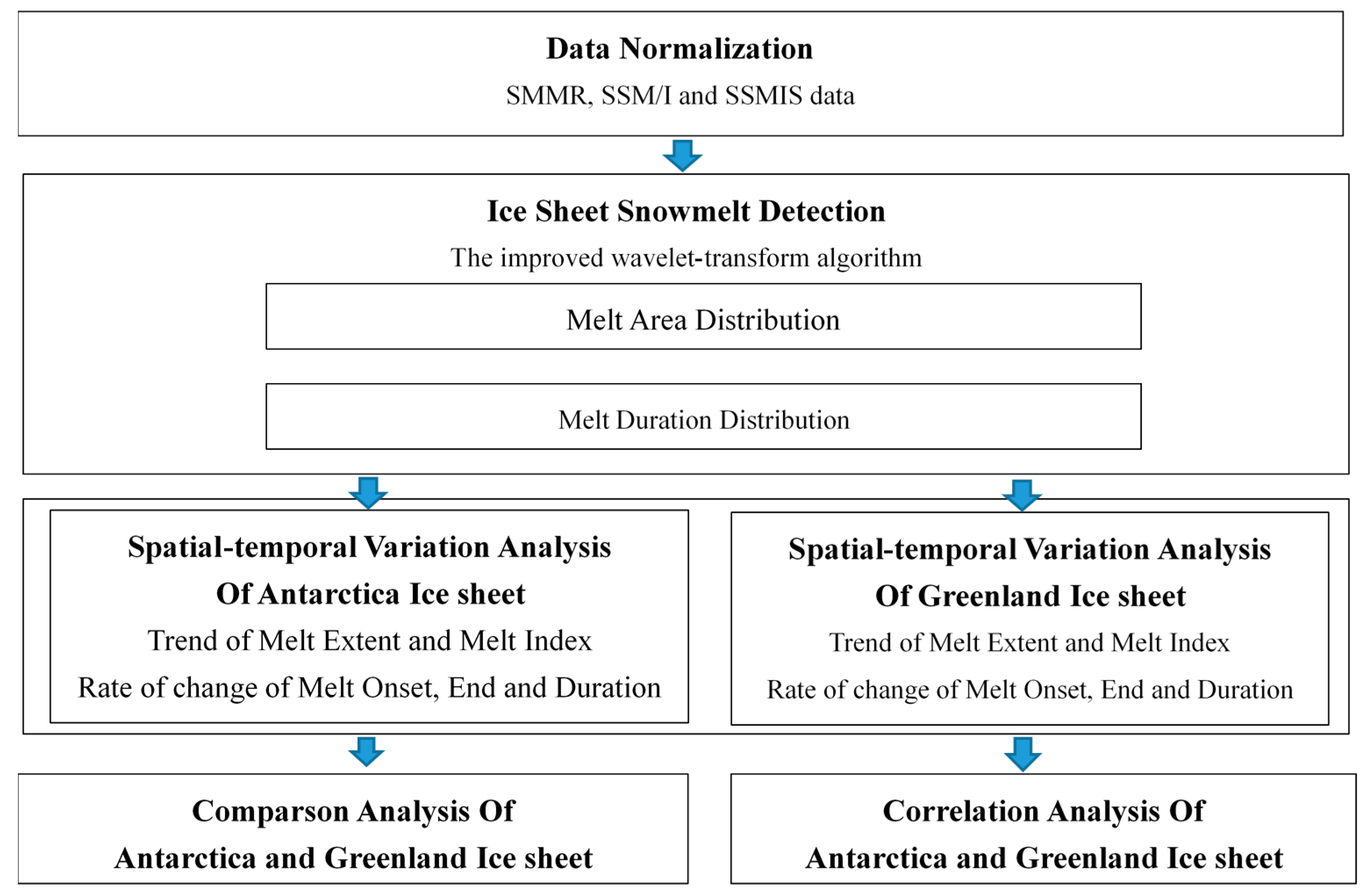
After data normalization, the SMMR and SSM/I datasets were processed using the improved wavelet-transform algorithm for ice sheet snowmelt detection [25]. In this method, to determine the optimal threshold for classification of wet and dry snow, we improved the bi-Gaussian-based threshold method [2], and used a generalized Gaussian-based adaptive optimal threshold algorithm, which makes the threshold determination more adaptive and flexible [25].
In addition, to obtain a more accurate classification threshold for dry and wet snow in Antarctica, the following more refined sampling scheme, which is based on the stability of a region regarding climate change, was proposed (noting that there is no need to do that for Greenland because all regions were used to calculate the threshold): the extraction of fewer dry snow samples in stable regions, and more samples in unstable regions. This principle of accounting for spatial variation in the wet-snow threshold was also used to extract the wet-snow pixels—that is, more samples were extracted for the regions experiencing relatively strong climate change, such as west Antarctica, coastal regions, low-latitude and low-altitude regions, and certain ice shelves (such as the Ross Ice Shelf), and fewer samples were also extracted for the Antarctic regions with relatively little climate change, such as East Antarctica and inland, high-latitude, and high-altitude regions.
In order to validate our classification results based on the sampling scheme in ice sheets of Antarctica, the near-surface air temperature data at several automated weather stations (AWS) with more than 10 years of observations were used. Since AWS do not cover the same area observed by large-scale remote sensing, they do not quite measure the same thing as our method. Therefore, to minimize the influence of the environment, we chose AWS-located areas where the spatial gradients were relatively simple, meaning that their temperature data should reflect average temperatures over large areas. We used the Radarsat Antarctic Mapping Project Digital Elevation Model, 1 km data to calculate the standard deviation, minimum and maximum heights in a 625 km2 area around the AWS to determine spatial complexity of the terrain, selecting the AWS stations shown in Table 2. The daily mean air temperature data, together with the corresponding daily results were used to quantitatively validate the snowmelt detection results of the method. For processing the AWS data, we chose the daily mean air temperature data from the summer months (November–March) in Antarctica. The total number of days, N (i.e., the total number of daily mean air temperature data) chosen in each AWS can be seen in Table 2. The daily mean air temperature data are made up of the mean of three daily maximum air temperatures—a daily mean maximum air temperature above 0 °C was regarded as a snowmelt occurrence. A melt day is where the daily mean maximum air temperature is above 0 °C, and a non-melt day is where the daily mean maximum air temperature is below 0 °C. We compared the results from the AWS and our method using: (1) Fraction of true positives (TP), that is, the melt days that were correctly detected, PTP = TP/N; (2) Fraction of true negatives (TN), that is, non-melt days that were correctly detected, PTN = TN/N; (3) Correct Detection Rate (CDR), that is, the ratio of correct detection results to the total number of detection results (or the total number of temperature data), CDR = (TP + TN)/N. The statistical analysis is shown in Table 3. The TP values of the method are very small near the AWS Butler, Amery G3, and Cape Bird, being 8% 5%, and 9%, respectively. This is because the number of melt days recorded by these AWS are very few, accounting for only 10%, 6%, and 8% of their respective records, and so TN also needed to be considered, as it is in the CDR statistic. Most CDR exceeds 80%, indicating that the sampling scheme is effective.
2.2.2. Analysis Method of Spatial-Temporal Variation of Antarctica and Greenland Ice Sheet Snowmelt
After ice sheet snowmelt detection in Antarctica and Greenland, the onset date, end date, and duration maps of the 37 years of ice sheet snowmelt were obtained. Because there is a 28-day data gap in the SSM/I data during December 1987, no Antarctic ice sheet freeze–thaw information was extracted between 1987 and 1988.
To quantitatively analyze the long time-series ice sheet snowmelt changes in Antarctica and Greenland from 1978 to 2014, three indicators were used to study the interannual temporal and spatial variability of the Antarctica and Greenland ice sheet snowmelt: melt extent (ME) and melt index (MI) [11]. These three indicators are given as follows:
where A is the area of one grid cell for the SSM/I data, MDi is melt duration (the number of melt days) within a year for pixel i, and N is the total number of melt pixels for the year. The melt extent represents the Antarctica and Greenland ice sheet melt areas for the year. To a certain degree, the melt index reflects the intensity of the Antarctica and Greenland ice sheet melt for the year. The MI is determined by two factors: the melt extent and melt duration.
To characterize the interannual change in the timing of the Antarctica and Greenland ice sheet melt, three new parameters that can detect the tendency of the snowmelt to change were proposed based on the time series regression analysis of the melt onset date, end date, and duration. These parameters are the change rates of the melt onset date, end date, and duration.
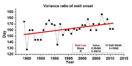
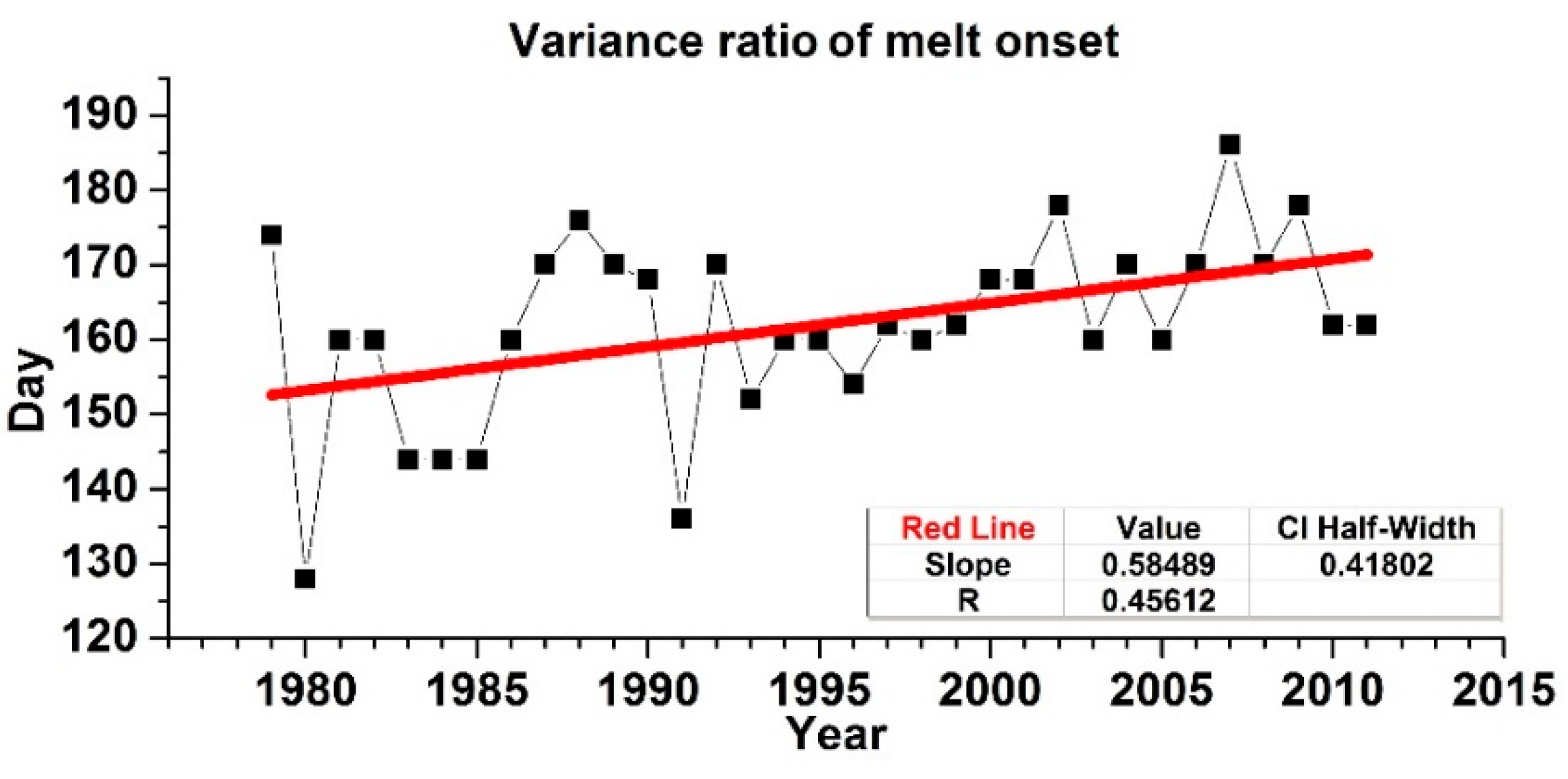
Here, July 1 and June 30 of the following year are defined as the first and last day, respectively, of the Antarctic year; and January 1 and December 31 are defined as the first and last days, respectively, of the Greenland year. The steps for estimating the rate of change in the snowmelt onset date, which is taken as an example of the newly proposed parameters, are listed below. (1) The annual snowmelt onset date for the entire Antarctic ice sheet for each of 37 Antarctic years (1978–2014) was derived using an improved wavelet transform algorithm for ice sheet freeze–thaw detection. (2) A least squares fitting was conducted, and the linear trend of the annual melt onset date for a pixel was obtained using the red solid line shown in Figure 1, in which the horizontal axis represents years from 1978 to 2014, and the vertical axis shows the onset day of the annual snowmelt. The slope of the line represents the rate of change in the melt onset date. (3) A change analysis based on linear trends was performed. A positive rate of change (positive slope) in the snowmelt onset date indicates that the melt onset date has been delayed, and a negative rate of change means that the melt onset date has been moved forward. The rate of change in the melt onset date for the entire Antarctic ice sheet is approximately 0.6 days per year, as shown in Figure 2, which indicates that there has been an average 0.6-day delay per year in the melt onset date in Antarctica from 1978 to 2014. The same method described above can be used to estimate the rate of change in the snowmelt end date and duration.
Based on the typical and newly proposed parameters for the detection of changes in ice sheet snowmelt, the maps of the Antarctica and Greenland ice sheet snowmelt extent (ME), the melt index (MI), and the rates of change (RC) in the melt onset date, end date, and duration during the period of 1978 to 2014 were derived.
The overall process of snowmelt detection and analysis of Antarctica and Greenland ice sheets introduced above is shown in Figure 2.
3. Results
Using the new proposed parameters regarding the snowmelt duration, the distribution of RC of the snowmelt duration in the two ice sheets’ snowmelt during 1978 to 2014 was obtained. To achieve statistical significance, places with infrequent snowmelt events from 1978 to 2014 (the number of occurrences of melt events is less than 15) were not included in the statistical analysis.
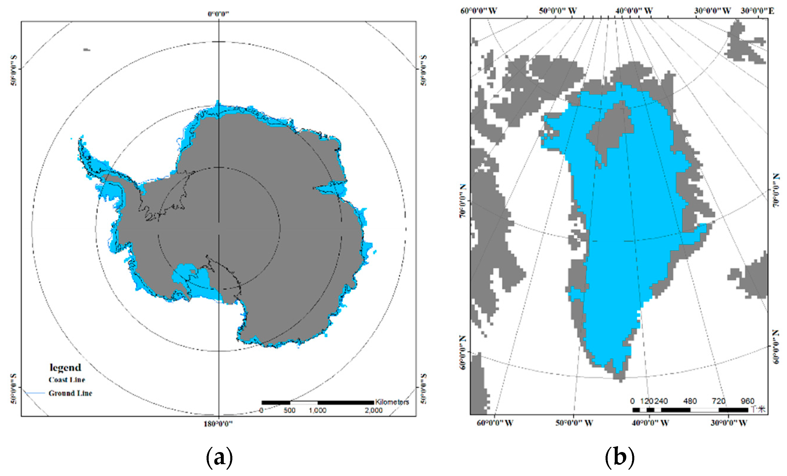
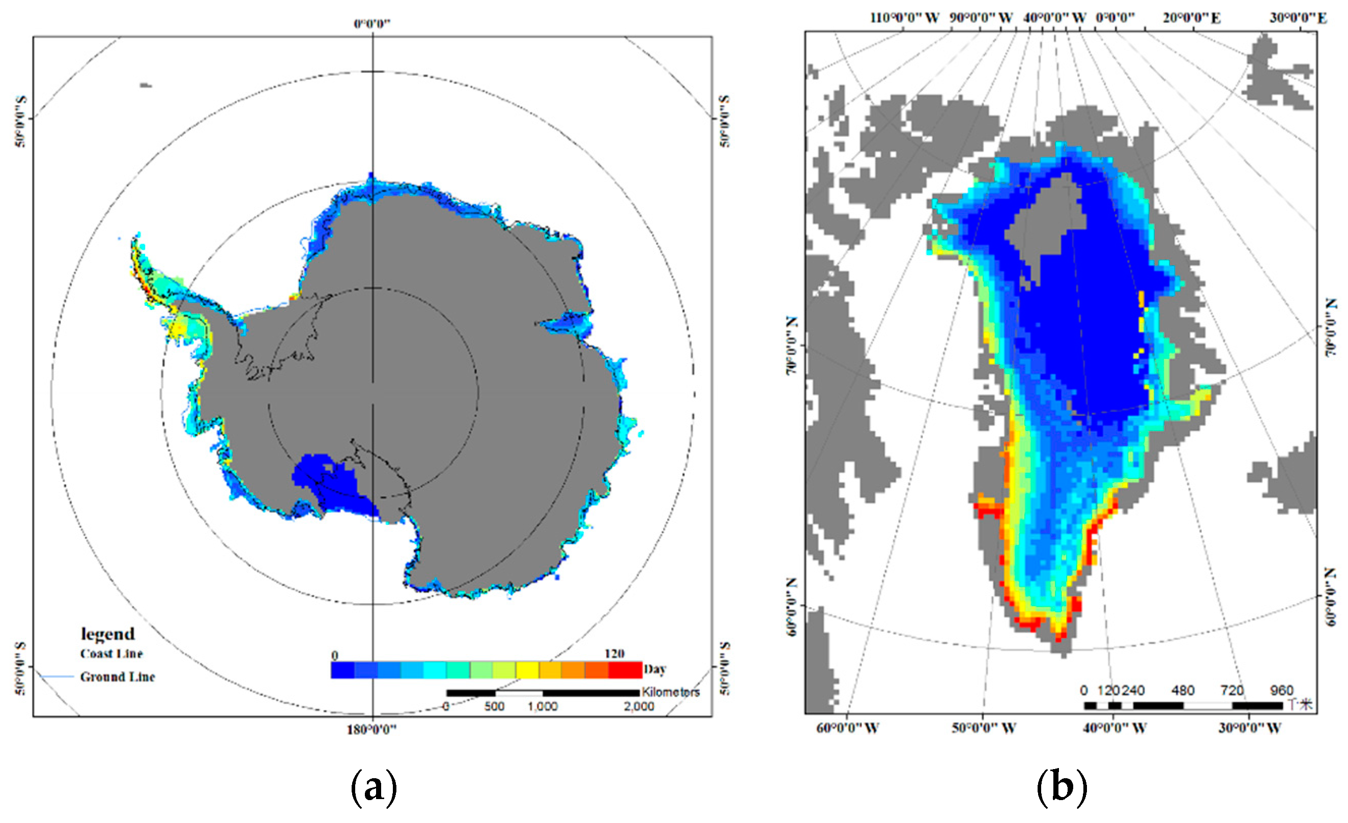
Figure 3a shows that, in ice sheets of Antarctica, there was an average melting area of 1,098,000 km2 over 1978–2014, which is about 10% of the total Antarctican ice sheet area. Moreover, the average melt duration was about 32 days per year during 1978–2014, and more than 80% of the melt area experienced melting for at least 10 days per year (Figure 4a). The absolute seasonal melt area of the Greenland ice sheet is smaller than that of Antarctica, and the average area affected was 764,000 km2 for 1978–2014 (see Figure 3b). However, the relative melt area of the Greenland ice sheet is much larger than that of Antarctica (see Figure 4b). In the Greenland ice sheets, more than 60% of the melt area melted for at least 10 days per year, with an areal average of 28 days per year (Figure 4b).
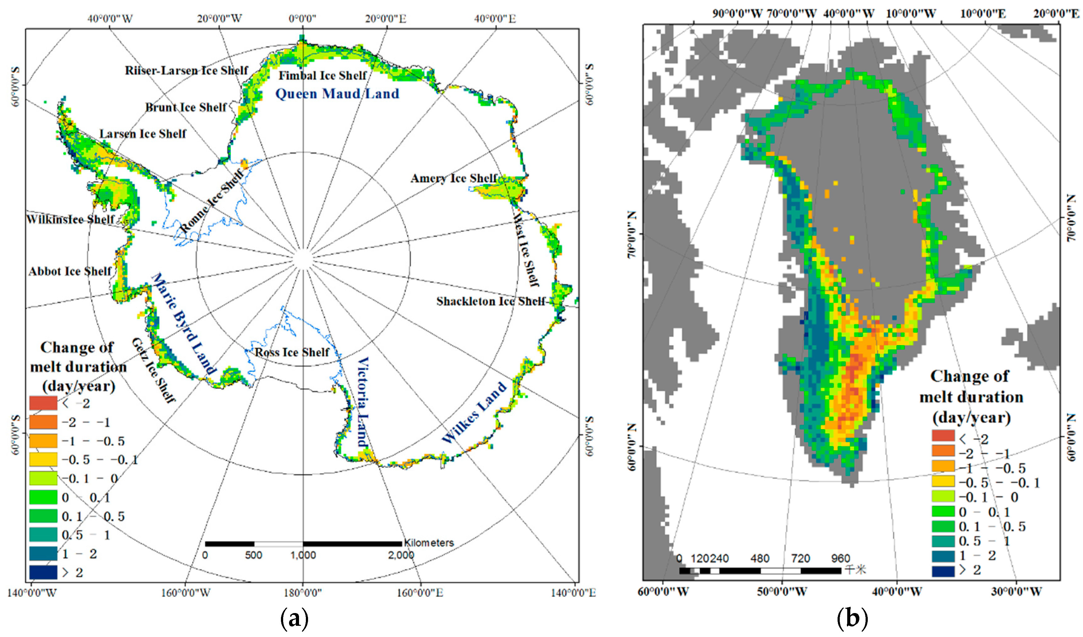
Figure 5 shows the distribution of trends in the change in melt duration in Antarctica and Greenland during 1978–2014. Green to deep blue colors show areas with rates that are greater than zero, indicating that the duration was lengthened, whereas yellow to red colors indicate that the duration was shortened. From the statistical analysis, in Antarctica, the melt duration was extended and shortened in approximately 34% and 66% of the melt areas, respectively; thus, the melt duration in Antarctica displayed a tendency toward shortening for most areas. In Greenland, the melt duration was extended and shortened in approximately 61% and 38% of the melt areas, respectively, which indicated that the melt duration in Greenland displayed a tendency toward extending for most areas.
4. Discussion
4.1. Comparison Analysis of Ice Sheet Snowmelt in Antarctica and Greenland
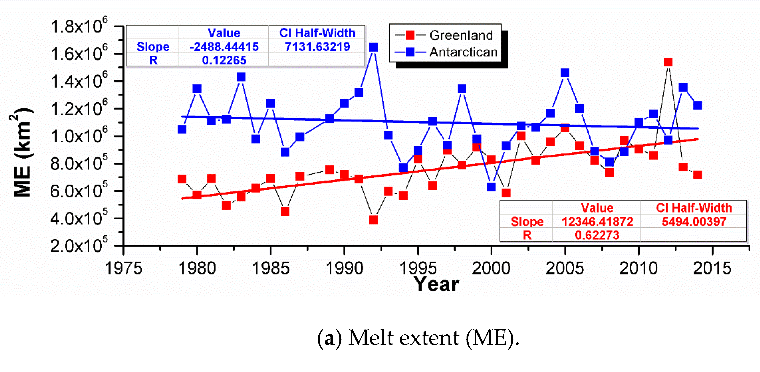
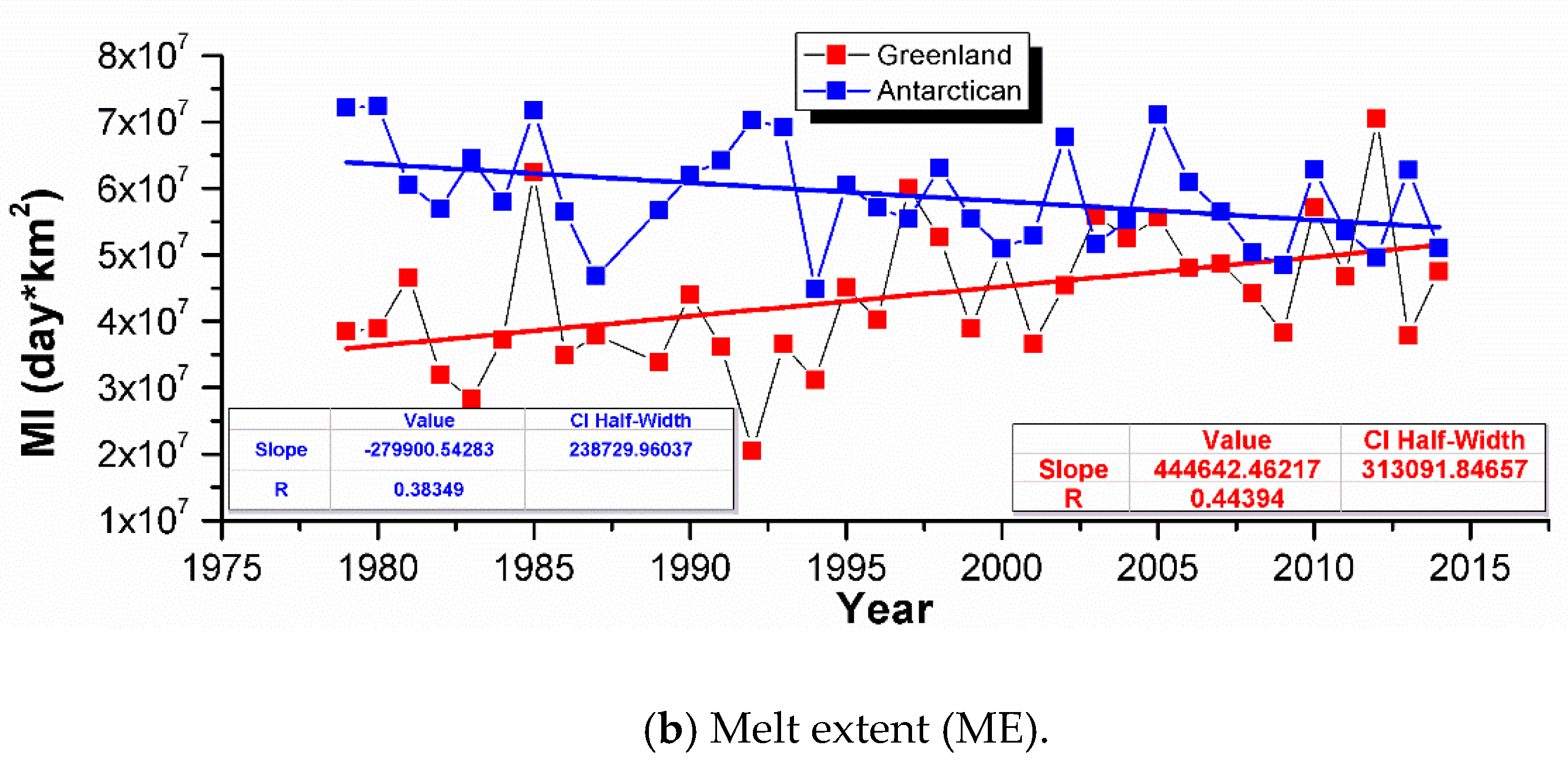
To reveal interannual changes in the spatial and temporal characteristics of the snowmelt in Antarctica and Greenland during 1978–2014, linear regression analyses of the ME and MI were conducted, and the results are plotted as red lines in Figure 6. During 1978–2014, the total Antarctic ME decreased by 2488.44 ± 7131.63 km2/year, and the MI decreased by 279900.54 ± 238729.96 day*km2/year. Generally, this result signifies a slightly reduced snowmelt overall in the Antarctic regions during 1978–2014. The Greenland ME increased by 12346.42 ± 5494.00 km2/year and the MI increased by 444642.46 ± 313091.85 day*km2/year during 1978–2014, which indicated that the snowmelt of Greenland ice sheets was intensified during this period.
From the analysis above, we can see that the snowmelt trend in Greenland was quite the opposite of that in Antarctica during 1978 to 2014—in Antarctica, the snowmelt of ice sheets was reduced slightly, and in Greenland, the intensified snowmelt of ice sheets happened during this period.
4.2. Correlation Analysis of Ice Sheet Snowmelt in Antarctica and Greenland
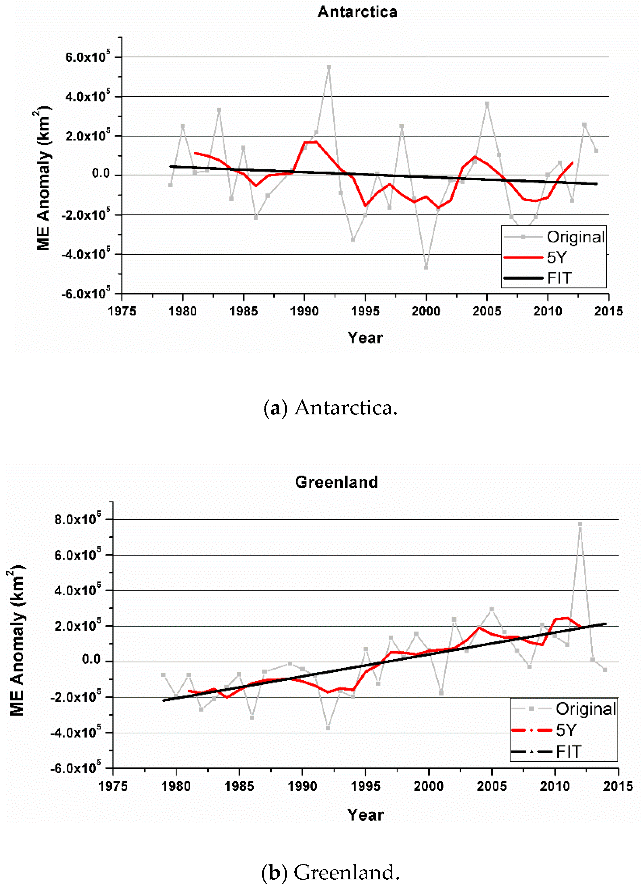
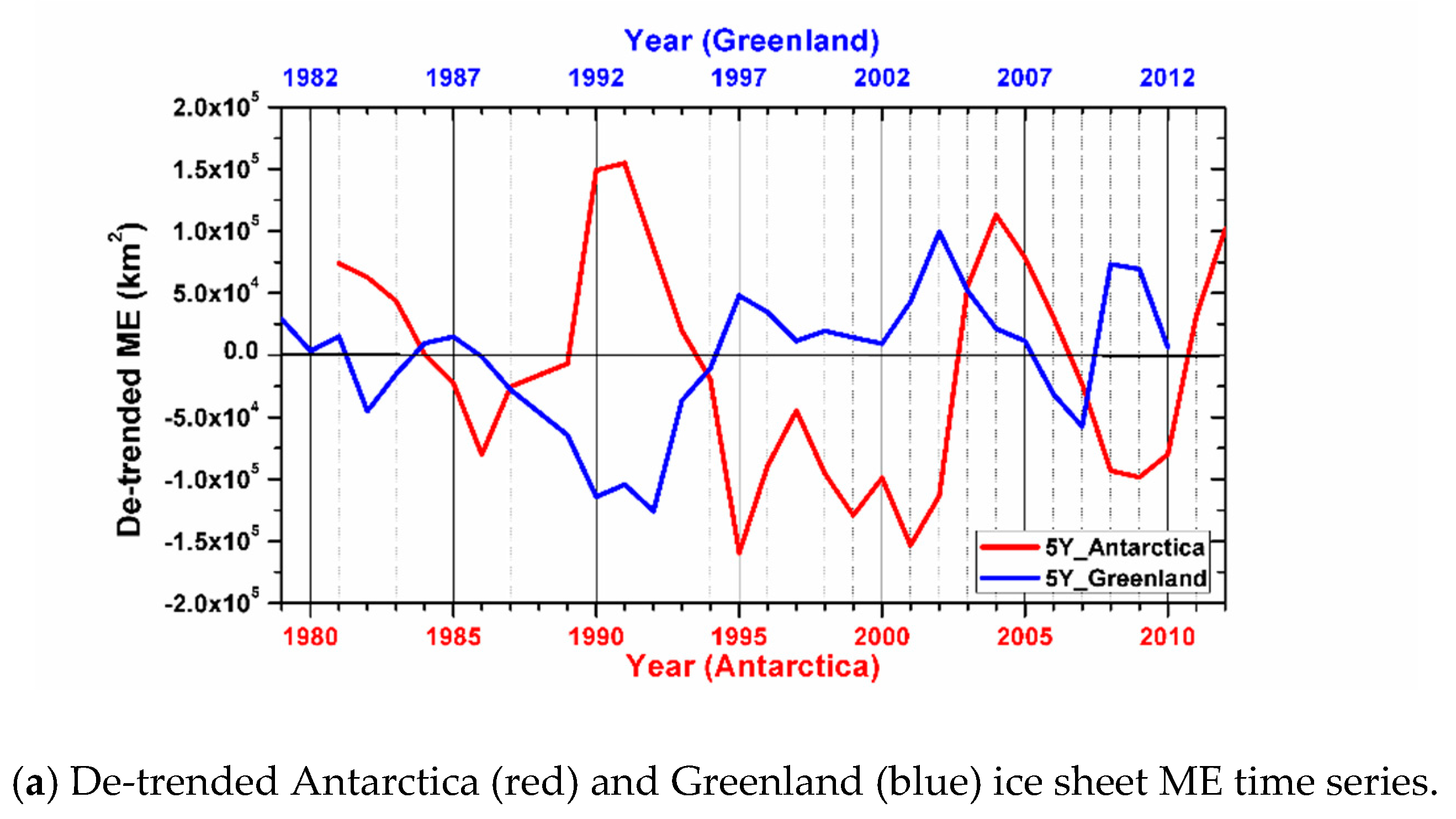
In our correlation analysis of ice sheet snowmelt between Antarctica and Greenland, we used the annual ME (Figure 7). The time series of ME were decomposed into linear trend and residual variability. Furthermore, the residual de-trended data was smoothed by applying a five-year running average to isolate multi-year scale variability (Figure 8a). We found the residual de-trended series to be highly anti-correlated when the ME inter-annual variation of Antarctican ice sheets was two years ahead of that of Greenland ice sheets (see Figure 8a). The correlation coefficient was r = −0.62, with statistical significance at the 95% level of confidence (p < 0.05).
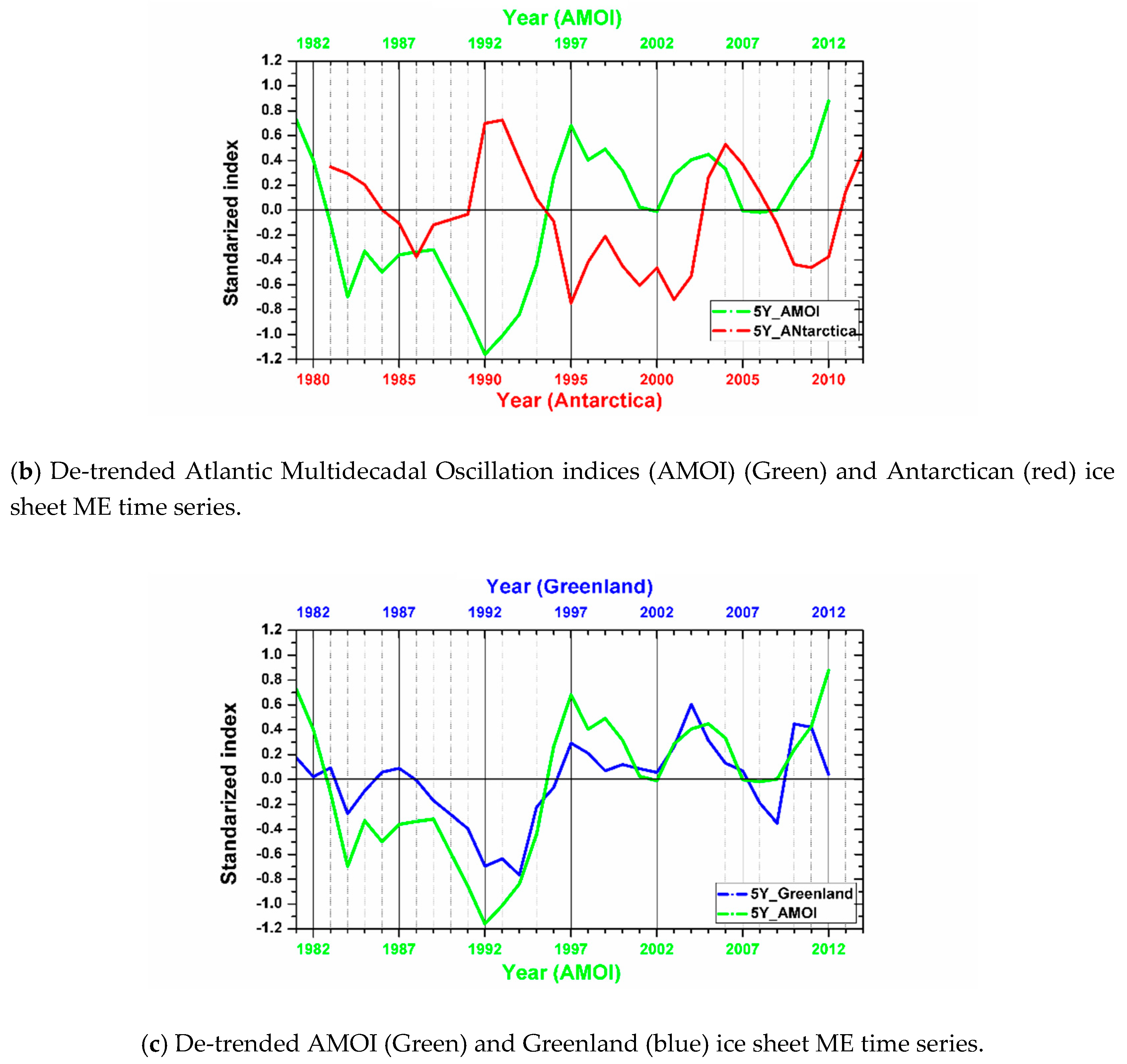
The snowmelt variability of the Greenland and Antarctic ice sheets is consistent with the seesaw pattern of the Arctic and Antarctic surface air temperatures. Considering that the bipolar seesaw pattern is well-correlated with the AMO signal [26,27,28], we thus investigated the relationship between the AMO change and snowmelt change of polar ice sheets. The result of correlation analysis between Antarctican ice sheets and AMO also shows that when inter-annual variation of ME in Antarctica ice sheets is two years ahead of that of the AMO index, the residual de-trended series are highly anti-correlated (see Figure 8b). The correlation coefficients are r = −0.5646 for the five-year averages, with statistical significance at the 99% level of confidence (p < 0.01). However, the Greenland (Antarctic) detrended ME was highly correlated with the AMO index, with the correlation coefficients r = 0.7869 and the statistical significance at the 99% level of confidence (p < 0.01) for the five-year averages (see Figure 8c). The high correlation (anti-correlation) between the AMO and Greenland (Antarctic) ice sheet suggests a link between the snowmelt variability of the polar ice sheet and the condition of the Atlantic Ocean. The AMO signal is usually defined from the patterns of sea surface temperature (SST) variability in the North Atlantic. In this way, the correlation analysis above indicates that an increasing (decreasing) SST in the North Atlantic directly influences a melt’s increase (or decrease) of Greenland ice sheets. However, it shows that the SST variability in the North Atlantic has a lag of two years to the snowmelt of Antarctican ice sheets. The reason could be related to Atlantic Meridional Overturning Circulation (AMOC), which generally leads to the origin of the AMO [29]. It is well-known as a possible link between the climate variability of the Northern Hemisphere (NH) and the Southern Hemisphere (SH) that the AMOC transports heat northward in both hemispheres. Buoyancy loss at its upper surface drive convection in the ocean, primarily at high latitudes. In this way, wind stress along the Antarctic Circumpolar Current dominates the upwelling around Antarctica. The wind stress thus draws the deep and intermediate waters to the surface. Then, the waters come into contact with the atmosphere, and are heated by the sun. Subsequently, the warm waters are transported away from the Antarctic area to the equatorial area by the Atlantic surface current. Through additional warming in the equator, the warm waters are further transported to the Arctic area. This transport process could take a long time, which is why the SST variability in the North Atlantic has a lag of two years to the snowmelt of the Antarctican ice sheet. During the transportation process, on the one hand, heat is being continuously transported to the northern hemisphere and northward to the Arctic from the Southern Ocean and Antarctica, and it could be lost in the Southern Ocean and Antarctica. In this way, the more efficient the transportation process, the greater is the warming in the NH and the cooling in the SH. In other words, when AMOC strengthens, northward oceanic heat flux could increase, which could lead to a warming trend in the Arctic and a cooling trend in Antarctica. This explains why the snowmelt variability of Antarctican ice sheets is anti-correlated with AMO variability and that of Greenland ice sheets.
The above analysis has shown an impact of oceans on the correlation between the Antarctican and Greenland ice sheet snowmelt. Besides, the atmosphere may also play a role in the anti-correlation. When cooling in NH, it could lead to a decrease of snowmelt in Greenland. Meanwhile, the NH and tropics cooling drove the weakening of the SH westerly jet, causing broad warming at SH high latitudes [30], and it might also have caused an increase of snowmelt in Antarctican ice sheets. Conversely, warming in NH could lead to an increase of snowmelt in Greenland. Furthermore, NH and tropical warming initiated and drove along with Antarctic ozone depletion, as well as the strengthening of the SH westerly jet, causing broad cooling at SH high latitudes [30]. Then, it might cause a decreasing of snowmelt in Antarctican ice sheets.
5. Conclusions
In this paper, based on an improved ice sheet snowmelt detection algorithm and several new proposed change detection parameters, as well as 37 years of spaceborne microwave radiometer datasets (1978–2014), polar ice sheet snowmelt dynamics were monitored and analyzed. Generally, during 1978 to 2014, the change in the intensity of polar ice sheet snowmelt manifested an opposite tendency—the snowmelt of ice sheets was reduced slightly in Antarctica, and intensified snowmelt of ice sheets happened during this period in Greenland. The feature of snowmelt in each polar ice sheet is that most of Greenland ice sheets experienced an earlier onset of melt and later freeze-up dates, resulting in increases in length of the melt season; however, both the onset and end dates of the snowmelt in Antarctica tended to be delayed with shortened melt duration. Moreover, we found that the de-trended snowmelt change in Greenland and Antarctican ice sheets varied in anti-correlation patterns—that is, when the snowmelt in the Antarctica decreased, Greenland ice sheets increased two years later, and when the snowmelt in Antarctica increased, Greenland ice sheets decreased two years later. The Antarctican (Greenland) de-trended snowmelt was also highly anti-correlated (correlated) with the AMO index. This suggested that the AMOC could be a possible link between the snowmelt variability of the Greenland and Antarctican ice sheets. When AMOC strengthens (or weakens), northward oceanic heat flux increases (or decreases), which could warm (or cool) the Arctic, but cool (or warm) Antarctica, and then cause the snowmelt to increase (or decrease) in Greenland and decrease (or increase) in Antarctica.
Author Contributions
Conceptualization, L.L. and X.L.; methodology, L.L.; validation, L.L.; formal analysis, L.L.; writing—original draft preparation, L.L.; writing—review and editing, F.Z.; supervision, X.L.; funding acquisition, X.L.
Funding
This research was funded by the Strategic Priority Research Program of the Chinese Academy of Sciences, grant number XDA19070202 and National Program on Key Research Project, grant number 2016YFA0600302.
Conflicts of Interest
The authors declare no conflict of interest.
References
- Meier, M.F. Ice, Climate and sea level. Do we know what is happening? In Ice in The Climate System; Peltier, W.R., Ed.; Springer Link: Berlin/Heidelberg, Germany, 1993; pp. 141–160. [Google Scholar]
- Liu, H.; Wang, L.; Jezek, K. Wavelet-transform based edge detection approach to derivation of snowmelt onset, end and duration from satellite passive microwave measurements. Int. J. Remote Sens. 2005, 26, 4639–4660. [Google Scholar] [CrossRef]
- Haggerty, J.A.; Curry, J.A. Variability of sea ice emissivity estimated from airborne passive microwave measurements during FIRE SHEBA. J. Geophys. Res. Atmos. 2001, 106, 15265–15277. [Google Scholar] [CrossRef]
- Lee, S.-M.; Sohn, B.-J. Retrieving the refractive index, emissivity, and surface temperature of polar sea ice from 6.9 GHz microwave measurements: A theoretical development. J. Geophys. Res. Atmos. 2015, 120, 2293–2305. [Google Scholar] [CrossRef]
- Skofronick-Jackson, G.M.; Gasiewski, A.J.; Wang, J.R. Influence of microphysical cloud parameterizations on microwave brightness temperatures. IEEE Trans. Geosci. Remote Sens. 2002, 40, 187–196. [Google Scholar] [CrossRef]
- Zwally, H.J.; Gloersen, P. Passive microwave images of polar regions and research applications. Polar Rec. 1977, 18, 431–450. [Google Scholar] [CrossRef]
- Ulaby, F.T.; Moore, R.K.; Fung, A. Microwave Remote Sensing: Active and Passive; From theory to application; Artech House: Norwood, MA, USA, 1986; Volume III. [Google Scholar]
- Mote, T.L.; Anderson, M.R.; Kuivenen, K.C.; Rowe, C.M. Passive microwave-derived spatial and temporal variations of summer melt on Greenland ice sheet. Ann. Glaciol. 1993, 17, 233–238. [Google Scholar] [CrossRef]
- Zwally, H.J.; Fiegles, S. Extent and duration of Antarctic surface melting. J. Glaciol. 1994, 40, 463–476. [Google Scholar] [CrossRef]
- Steffen, K.; Abdalati, W.; Stroeve, J. Climate sensitivity studies of the Greenland ice sheet using satellite AVHRR, SMMR, SSM/I and in situ data. Meteorol. Atmos. Phys. 1993, 51, 239–258. [Google Scholar] [CrossRef] [Green Version]
- Abdalati, W.; Steffen, K. Greenland Ice Sheet melt extent: 1979–1999. J. Geophys. Res. 2001, 106, 33983–33988. [Google Scholar] [CrossRef]
- Takala, M.; Pulliainen, J.; Huttunen, M.; Hallikainen, M. Estimation of the beginning of snow melt period using SSM/I data. In Proceedings of the IEEE International Geoscience and Remote Sensing Symposium 2003 (IGARSS), Toulouse, France, 21–25 July 2003. [Google Scholar]
- Joshi, M.; Merry, C.J.; Jezek, K.C.; Bolzan, J.F. An edge detection technique to estimate melt duration, season and melt extent on the Greenland ice sheet using passive microwave data. Geophys. Res. Lett. 2001, 28, 3497–3500. [Google Scholar] [CrossRef]
- Liu, H.; Wang, L.; Jezek, K. Spatio-temporal variations of snow melt zones in Antarctic Ice Sheet derived from satellite SMMR and SSM/I data (1978-2004). J. Geophys. Res. 2006, 111, F01003. [Google Scholar] [CrossRef]
- Aschraft, I.S.; Long, D.G. Comparison of methods for melt detection over Greenland using active and passive microwave measurements. Int. J. Remote Sens. 2006, 27, 2469–2488. [Google Scholar]
- Torinesi, O.; Fily, M.; Genthon, C. Variability and trends of the summer melt period of Antarctic Ice margins since 1980 from Microwave sensors. J. Clim. 2003, 16, 1047–1060. [Google Scholar] [CrossRef]
- Tedesco, M. Assessment and development of snowmelt retrieval algorithms over Antarctica from K-band spaceborne brightness temperature (1979–2008). Remote Sens. Environ. 2009, 113, 979–997. [Google Scholar] [CrossRef]
- Tedesco, M.; Abdalati, W.; Zwally, H.J. Persistent surface snowmelt over Antarctica (1987–2006) from 19.35 GHz brightness temperatures. Geophys. Res. Lett. 2007, 34. [Google Scholar] [CrossRef]
- Narvekar, P.S.; Heygster, G.; Jackson, T.J.; Bindlish, R.; Macelloni, G.; Notholt, J. Passive Polarimetric Microwave Signatures Observed Over Antarctica. IEEE Trans. Geosci. Remote Sens. 2010, 48, 1059–1075. [Google Scholar] [CrossRef]
- Mote, T.L. Greenland surface melt trends 1973-2007: Evidence of a large increase in 2007. Geophys. Res. Lett. 2007, 34, L22507. [Google Scholar] [CrossRef]
- Knowles, K.; Njoku, E.G.; Armstrong, R.; Brodzik, M. Nimbus-7 SMMR Pathfinder Daily EASE-Grid Brightness Temperatures; NASA National Snow and Ice Data Center Distributed Active Archive Center: Boulder, CO, USA, 2000; Version 1. [Indicate subset used]. [Google Scholar] [CrossRef]
- Maslanik, J.; Stroeve, J. DMSP SSM/I-SSMIS Daily Polar Gridded Brightness Temperatures; NASA National Snow and Ice Data Center Distributed Active Archive Center: Boulder, CO, USA, 2004; Version 4. [Indicate subset used]. (Updated 2016). [Google Scholar] [CrossRef]
- Jezek, K.C.; Merry, C.A.; Cavalieri, D.; Bedner, J.; Wilson, D.; Lampkin, D.J. Comparison Between SMMR and SSM/I Passive Microwave Data Collected Over the Antarctic Ice Sheet; Byrd Polar Research Center Tech Rep; Ohio State University: Columbus, OH, USA, 1991; pp. 91–103. [Google Scholar]
- Abdalati, W.; Steffen, K.; Otto, C.; Jezek, K.C. Comparison of brightness temperatures from SMI instruments on the DMSP F8 and F11 satellites for Antarctica and the Greenland ice sheet. Int. J. Remote Sens. 1995, 16, 1223–1229. [Google Scholar] [CrossRef]
- Liang, L.; Guo, H.; Li, X.; Cheng, X.; Wang, X. Automated Snowmelt Detection Using Microwave Radiometer Measurements. Polar Res. 2013, 32, 19746. [Google Scholar] [CrossRef]
- Folland, C.K.; Palmer, T.; Parker, D.E. Sahel rainfall and worldwide sea temperatures. Nature 1986, 320, 602–607. [Google Scholar] [CrossRef]
- Knight, J.R.; Folland, C.K.; Scaife, A.A. Climate impact of the Atlantic Multidecadal Oscillation. Geophys. Res. Lett. 2006, 33, L17706. [Google Scholar] [CrossRef]
- Knight, J.R. The Atlantic Multidecadal Oscillation inferred from the forced climate response in coupled general circulation models. J. Clim. 2009, 22, 1610–1625. [Google Scholar] [CrossRef]
- Knight, J.R.; Allan, R.J.; Folland, C.K.; Vellinga, M.; Mann, M. A signature of the persistence natural thermohaline circulation cycle in observed climate. Geophys. Res. Lett. 2005, 32, L20708. [Google Scholar] [CrossRef]
- Wang, Z.; Zhang, X.; Guan, Z.; Sun, B.; Yang, X.; Liu, C. An atmospheric origin of the multi-decadal bipolar seesaw. Sci. Rep. 2015, 5, 8909. [Google Scholar] [CrossRef] [PubMed]
Figure 1.
Rate of change of the Antarctic melt onset date.

Figure 2.
The flowchart of snowmelt detection and analysis of Antarctican ice sheets.

Figure 3.
Average annual melt extent from 1978 to 2014 in (a) Antarctican and (b) Greenland ice sheets.
Figure 3.
Average annual melt extent from 1978 to 2014 in (a) Antarctican and (b) Greenland ice sheets.

Figure 4.
Average annual melt duration from 1978 to 2014 in (a) Antarctican and (b) Greenland ice sheets.
Figure 4.
Average annual melt duration from 1978 to 2014 in (a) Antarctican and (b) Greenland ice sheets.

Figure 5.
Distribution of the rate of change of the melt duration in (a) Antarctica and (b) Greenland during 1978–2014.
Figure 5.
Distribution of the rate of change of the melt duration in (a) Antarctica and (b) Greenland during 1978–2014.

Figure 6.
Interannual variation of (a) melt extent (ME) and (b) melt extent (ME) in Antarctica and Greenland with trend lines fitted for 1978–2014.
Figure 6.
Interannual variation of (a) melt extent (ME) and (b) melt extent (ME) in Antarctica and Greenland with trend lines fitted for 1978–2014.


Figure 7.
Melt extent (ME) anomaly with respect to the 1978–2014 average, its five-year running mean (red line) and the least square linear fit (thick black line) for the (a) Antarctica and (b) Greenland ice sheets.
Figure 7.
Melt extent (ME) anomaly with respect to the 1978–2014 average, its five-year running mean (red line) and the least square linear fit (thick black line) for the (a) Antarctica and (b) Greenland ice sheets.

Figure 8.
(a) De-trended Antarctica (red) and Greenland (blue) ice sheet ME time series smoothed by a five-year running average, while the time line of Antarctica is two years ahead of that of Greenland. (b) De-trended Atlantic Multidecadal Oscillation indices (AMOI) (Green) and Antarctican (red) ice sheet ME time series smoothed by a five-year running average, while the time line of Antarctica is two years ahead of that of Greenland. (c) De-trended AMOI (Green) and Greenland (blue) ice sheet ME time series smoothed by a five-year running average.


Table 1.
Regression coefficients for data adjustments between different sensors.
| Conversion | Slope | Intercept | Correlation Coefficient |
|---|---|---|---|
| SMMR 18 GHz Horizontal to SSM/I F-8 19 GHz Horizontal | 1.06 | −2.79 | R > 0.99 |
| SMM/I F-11 and F-13 19 GHz Horizontal to SSM/I F-8 19 GHz Horizontal | 1.008 | −1.17 | R > 0.99 |
| SSM/I F-17 19 Ghz horizontal to SSM/I F-8 19 Ghz horizontal | 1.0286 | −3.0094 | R > 0.99 |
Table 2.
Automatic weather stations (AWS) for the evaluation of the snowmelt detection methods. (The AWS can be obtained from http://amrc.ssec.wisc.edu/aws/).
Table 2.
Automatic weather stations (AWS) for the evaluation of the snowmelt detection methods. (The AWS can be obtained from http://amrc.ssec.wisc.edu/aws/).
| Station Name | Latitude/Longitude | Elevation | Dates | Days |
|---|---|---|---|---|
| Larsen Ice Shelf | 66.90S/60.60W | 50 m | 02/1983- | 2390 |
| Butler Island | 72.20S/60.34W | 91 m | 03/1986- | 2449 |
| Mount Siple | 73.198S/127.052W | 8 m | 01/1992- | 1761 |
| Amery G3 | 70.892S/69.873E | 84 m | 01/1999- | 1931 |
| Lanyon | 66.278S/110.797E | 390 m | 01/1991-12/2008 | 2015 |
| Cape Bird | 77.224S/166.440E | 38 m | 01/1999-12/2002 01/2009- | 1845 |
| Limbert | 75.420S/59.850 | 59 m | 01/1995-12/1997 01/2000-12/2002 01/2009- | 2111 |
Table 3.
Quantitative snowmelt detection results (in %).
| Automatic Weather Station | PTP | PTN | CDR |
|---|---|---|---|
| Mount Siple | 61 | 22 | 83 |
| Butler | 8 | 73 | 81 |
| Larsen Ice Shelf | 32 | 53 | 85 |
| Amery G3 | 5 | 83 | 88 |
| Lanyon | 45 | 35 | 80 |
| Cape Bird | 9 | 70 | 79 |
| Limbert | 30 | 52 | 82 |
© 2019 by the authors. Licensee MDPI, Basel, Switzerland. This article is an open access article distributed under the terms and conditions of the Creative Commons Attribution (CC BY) license (http://creativecommons.org/licenses/by/4.0/).
Share and Cite
MDPI and ACS Style
Liang, L.; Li, X.; Zheng, F. Spatio-Temporal Analysis of Ice Sheet Snowmelt in Antarctica and Greenland Using Microwave Radiometer Data. Remote Sens. 2019, 11, 1838. https://0-doi-org.brum.beds.ac.uk/10.3390/rs11161838
AMA Style
Liang L, Li X, Zheng F. Spatio-Temporal Analysis of Ice Sheet Snowmelt in Antarctica and Greenland Using Microwave Radiometer Data. Remote Sensing. 2019; 11(16):1838. https://0-doi-org.brum.beds.ac.uk/10.3390/rs11161838
Chicago/Turabian StyleLiang, Lei, Xinwu Li, and Fei Zheng. 2019. "Spatio-Temporal Analysis of Ice Sheet Snowmelt in Antarctica and Greenland Using Microwave Radiometer Data" Remote Sensing 11, no. 16: 1838. https://0-doi-org.brum.beds.ac.uk/10.3390/rs11161838
Note that from the first issue of 2016, this journal uses article numbers instead of page numbers. See further details here.