A Global Model for Estimating Tropospheric Delay and Weighted Mean Temperature Developed with Atmospheric Reanalysis Data from 1979 to 2017

Abstract

Precise modeling of tropospheric delay and weighted mean temperature (T_m) is critical for Global Navigation Satellite System (GNSS) positioning and meteorology. However, the model data in previous models cover a limited time span, which limits the accuracy of these models. Besides, the vertical variations of tropospheric delay and T_m are not perfectly modeled in previous studies, which affects the performance of height corrections. In this study, we used the European Centre for Medium-Range Weather Forecasts (ECMWF) ERA-Interim reanalysis from 1979 to 2017 to build a new empirical model. We first carefully modeled the lapse rates of tropospheric delay and T_m. Then we considered the temporal variations by linear trends, annual, and semi-annual variations and the spatial variations by grids. This new model can provide zenith hydrostatic delay (ZHD), zenith wet delay (ZWD), and T_m worldwide with a spatial resolution of 1° × 1°. We used the ECMWF ERA-Interim data and the radiosonde data in 2018 to validate this new model in comparison with the canonical GPT2w model. The results show that the new model has higher accuracies than the GPT2w model in all parameters. Particularly, this new model largely improves the accuracy in estimating ZHD and T_m at high-altitude (relative to the grid point height) regions.

1. Introduction

When Global Navigation Satellite System (GNSS) signals travel through the neutral atmosphere, they are bent and delayed due to atmospheric refractivity. The bending effect is usually neglected because it is very small when the elevation angle is larger than 10° [1]. However, the time delay induced excess ray path measurement can cause large errors in positioning results, which is referred to as the tropospheric delay in the GNSS community. The tropospheric delay can be divided into two components: a hydrostatic delay and a wet delay, and each component can be considered as the product of the zenith delay and its corresponding mapping function [2,3,4]. The tropospheric delay is an important error source in GNSS positioning, and accurate a priori tropospheric delay information, especially the zenith hydrostatic delay (ZHD), can improve estimates of station coordinates and zenith total delay [5]. Therefore, precise modeling of tropospheric delay is beneficial for GNSS positioning. Besides, the tropospheric delay contains important information about the neutral atmosphere, which can be used to remotely sense water vapor in the atmosphere. Literature study [3] derived the approximate relationship between zenith wet delay (ZWD) and precipitable water vapor (PWV). It also introduced the concept of weighted mean temperature (T_m), which is a crucial parameter in converting ZWD to PWV. Hence, GNSS-based water vapor measuring largely depends on the precise calculation of T_m.

For the tropospheric delay modeling, scientists have built many models up to now. Traditional tropospheric delay models [6,7] require meteorological observations from in situ sensors to calculate tropospheric delay. However, most GNSS stations are not equipped with meteorological sensors, empirical models are therefore needed. The existing empirical models are roughly divided into two types. The first type models meteorological parameters and uses traditional tropospheric delay models, e.g., the Saastamoinen model or similar models, to calculate tropospheric delay [8,9,10,11,12,13,14,15]. The second type models tropospheric delay directly, which provides empirical tropospheric delay free of meteorological parameters [16,17,18].

For the calculation of T_m, the traditional method requires vertical profiles of temperature and water vapor pressure. Such profiles are hard to acquire in reality, which greatly limits the development of GNSS meteorology. Literature studies [19,20] found that T_m has a high correlation with surface temperature (T_s) and proposed a linear relationship between them, which made the calculation of T_m easy. However, this method largely depends on T_s. Literature study [21] constructed the empirical Global Weighted Mean Temperature (GWMT) model, which contributed to the real-time calculation of PWV. Other T_m models have also been established [22,23,24,25,26,27,28], which has accelerated the development of GNSS meteorology.

However, none of the above listed models considered long-term linear trends in tropospheric delay and T_m modeling. Literature studies [29,30] reported that PWV have linear trends, suggesting that tropospheric delay and T_m may also have linear trends. If these linear trends are not taken into account while modeling, uncertainties will be introduced with time going on. Besides, previous models used model data usually covering a time span shorter than a decade. This limited time span is insufficient to simulate variations that are beyond the modeling period, and therefore lowers the accuracy of the model. In addition, some climate phenomena, e.g., the El Niño-Southern Oscillation (ENSO), can change the variation patterns [31], and if the time span is not long enough, the variation due to ENSO will not be simulated. Moreover, the vertical variations in tropospheric delay and T_m have not been perfectly modeled in previous studies, which limits the performance of height corrections. If the height corrections are not properly accounted for, large uncertainties will be introduced in the parameter estimates.

In this study, we used the European Centre for Medium-Range Weather Forecasts (ECMWF) ERA-Interim reanalysis from 1979 to 2017 to investigate the long-term variations in ZHD, ZWD, and T_m. Besides, we used the ECMWF ERA-Interim pressure level data to carefully model the vertical variations of ZHD, ZWD, and T_m to improve their height corrections. Finally, we used the same data to build a new global empirical model, which incorporates tropospheric delay correction and T_m calculation and can serve both GNSS positioning and meteorology.

2. Materials and Methods

2.1. European Centre for Medium-Range Weather Forecasts (ECMWF) ERA-Interim Reanalysis Data

ERA-Interim is an accurate global atmospheric reanalysis released by ECMWF. Compared with previous ECMWF reanalysis, e.g., the ERA-40 reanalysis, the ERA-Interim reanalysis has better quality by showing higher precision and higher spatiotemporal resolutions [32,33]. In this study, the ERA-Interim monthly pressure, temperature, and water vapor pressure on 37 pressure levels were used to calculate tropospheric parameters including ZHD, ZWD, and T_m. Since the Saastamoinen model [6] can accurately estimate ZHD with mm-level accuracy using in situ pressure [34], this model was used to compute ZHD with the ERA-Interim pressure data:

$$\mathrm{ZHD}=\frac{2.2768P}{1-0.00266\cos \left(2\phi \right)-0.00028h}$$

(1)

where P indicates the pressure (hPa), φ denotes the latitude (radian), and h is the height (km). ZWD and T_m are calculated using the following equations [2,19]:

$$\mathrm{ZWD}={10}^{-6}{{\displaystyle \int }}_h^{\infty }{N}_w\mathit{dh}$$

(2)

$$N_w=k_2^{\prime }\frac{e}{T}+k_3\frac{e}{T^2}$$

(3)

$${\mathrm{T}}_{\mathrm{m}}=\frac{{{\displaystyle \int }}_h^{\infty }\frac{e}{T}\mathit{dh}}{{{\displaystyle \int }}_h^{\infty }\frac{e}{T^2}\mathit{dh}}$$

(4)

where N_w is the wet refractivity, e and T denote the water vapor pressure (hPa) and the temperature (K), respectively, and $k_2^{\prime }{ \mathrm{and} k}_3$ are the atmospheric refractive index constants with the values of $22.97 \mathrm{K}/{\mathrm{hPa} \mathrm{and} 375,463 \mathrm{K}}^2/\mathrm{hPa}$ [35]. Using Equations (1)–(4), we can obtain ZHD, ZWD, and T_m at each pressure level.

The heights derived from the ECMWF ERA-Interim data are the geopotential heights, and we converted them to the ellipsoid heights in WGS-84, which are usually used by GNSS users. The surface height derived from the ECMWF was used as the height of each grid point. To obtain ZHD, ZWD, and T_m at the height of the grid point, we performed an interpolation or an extrapolation by assuming that these values vary linearly in the vertical direction within a short height range. Eventually, the ZHD, ZWD, and T_m at all the pressure levels below 10 km and at the height of the grid point from 1979 to 2018 were computed. We calculated these values at all the grid points on a global scale with a spatial resolution of 1° × 1°, which were then used to establish a new model and to validate the new model.

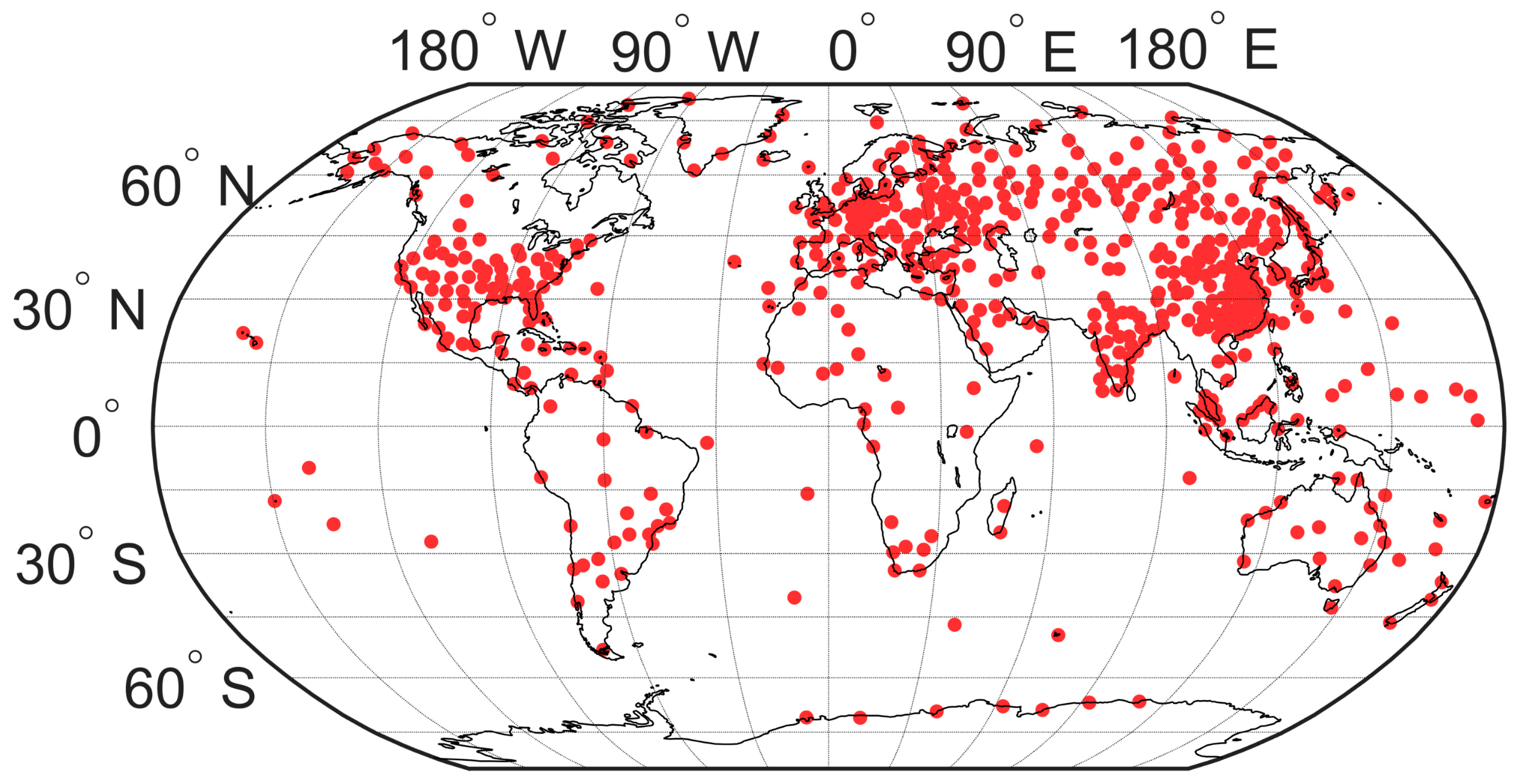
2.2. Radiosonde Data

Radiosonde data are important meteorological observations to evaluate other observations and model outputs. We obtained radiosonde data from the Integrated Global Radiosonde Archive (IGRA), which has provided high-quality sounding observations from more than 1500 radiosondes and sounding balloons distributed globally since the 1960s. The temporal interval of the radiosonde data is 12 h with the data available at 00:00 and 12:00 UTC. The radiosonde data provide meteorological profiles including pressure, temperature, relative humidity, etc., on certain pressure levels. We collected all available radiosonde data in 2018. The radiosonde stations with a lot of missing data were discarded. Eventually, we obtained in total 586 globally distributed radiosonde stations which are shown in Figure 1. The ZHD, ZWD, and T_m were computed using the radiosonde profiles and the same method as illustrated in Section 2.1. The height of the radiosonde data is also the geopotential height, which was converted to the ellipsoid height. These data were used to validate our model.

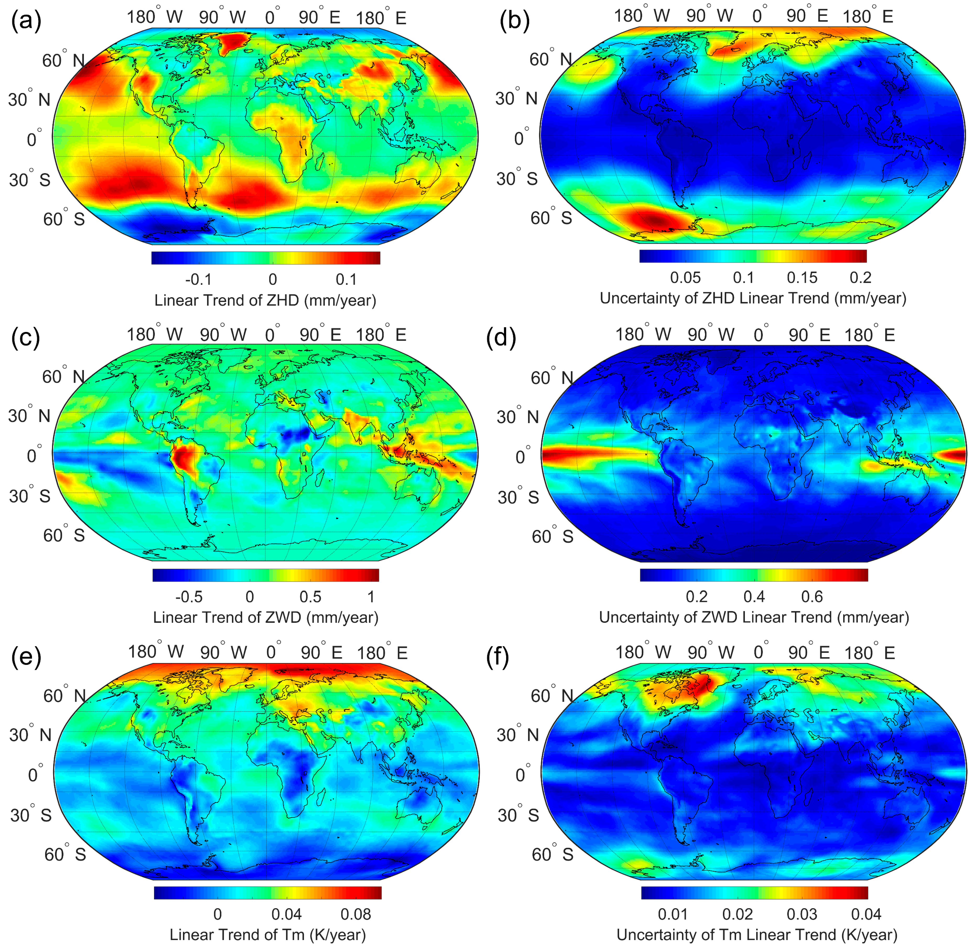
2.3. Linear Trends in Tropospheric Delay and T_m

We assumed that tropospheric delay and T_m have linear trends, which is in essence a first-order approximation of the long-term atmospheric behavior. To investigate their linear trends, we first selected four grid points at different latitudes and calculated their yearly ZHD, ZWD, and T_m from 1979 to 2017. We averaged the ECMWF ERA-Interim monthly data in each year to remove the seasonal variations. The yearly values and their linear trends at these grid points are presented in Figure 2. The linear trends in ZHD, ZWD, and T_m estimated at 95% confidence level are summarized in

Table 1. Linear trends in zenith hydrostatic delay (ZHD), zenith wet delay (ZWD), and weighted mean temperature (T_m) estimated at 95% confidence level, correlation coefficients, and p values at four grid points.

Longitude	Latitude	Tropospheric Parameter	Linear Trend	Correlation Coefficient	p Value
115°E	0°N	ZHD	−0.03 ± 0.02 mm/year	0.15	0.01
115°E	0°N	ZWD	0.70 ± 0.20 mm/year	0.52	2 × 10−7
115°E	0°N	Tm	−0.01 ± 0.01 K/year	0.08	0.08
115°E	30°N	ZHD	−0.03 ± 0.02 mm/year	0.25	1 × 10−3
115°E	30°N	ZWD	−0.05 ± 0.17 mm/year	0.01	0.51
115°E	30°N	Tm	0.03 ± 0.01 K/year	0.49	7 × 10−7
115°E	60°N	ZHD	0.01 ± 0.04 mm/year	0.01	0.60
115°E	60°N	ZWD	0.08 ± 0.09 mm/year	0.08	0.06
115°E	60°N	Tm	0.03 ± 0.02 K/year	0.23	2 × 10−3
115°E	90°N	ZHD	−0.08 ± 0.15 mm/year	0.03	0.28
115°E	90°N	ZWD	0.14 ± 0.04 mm/year	0.49	6 × 10−7
115°E	90°N	Tm	0.07 ± 0.02 K/year	0.57	2 × 10−8

. We also calculated the correlation coefficients and the p values from significance tests at these four grid points, which are also shown in Table 1. It shows that 7 of 12 p values are smaller than 0.05, and we thus inferred that ZHD, ZWD, and T_m time series at some grid points have linear trends.

We then calculated the linear trends, the corresponding uncertainties at the 95% confidence level, the correlation coefficients, and the p values for the ZHD, ZWD, and T_m time series over the globe. The global linear trends and the corresponding uncertainties are displayed in Figure 3, and the correlation coefficients and the p values are provided in Figure S1 of the Supplementary Material (SM). The statistics in Figure 3 show that the mean values of the global linear trends in ZHD, ZWD, and T_m are −0.006 mm/year, 0.048 mm/year, and 0.014 K/year, respectively; and the median values are −0.007 mm/year, 0.031 mm/year, and 0.008 K/year, respectively. The median values are close to the mean values, and we hence believe that the average values are convincing. The statistics in Figure S1 show that 16.9% (11,064 of 65,341), 44.1% (28,846 of 65,341), and 55.2% (36,073 of 65,341) of the grid points have p values smaller than 0.05 for ZHD, ZWD, and T_m, respectively. This indicates that the ZHD, ZWD, and T_m time series at the corresponding grid points exhibit linear variations. Therefore, we modeled the linear trends of ZHD, ZWD, and T_m in our new model.

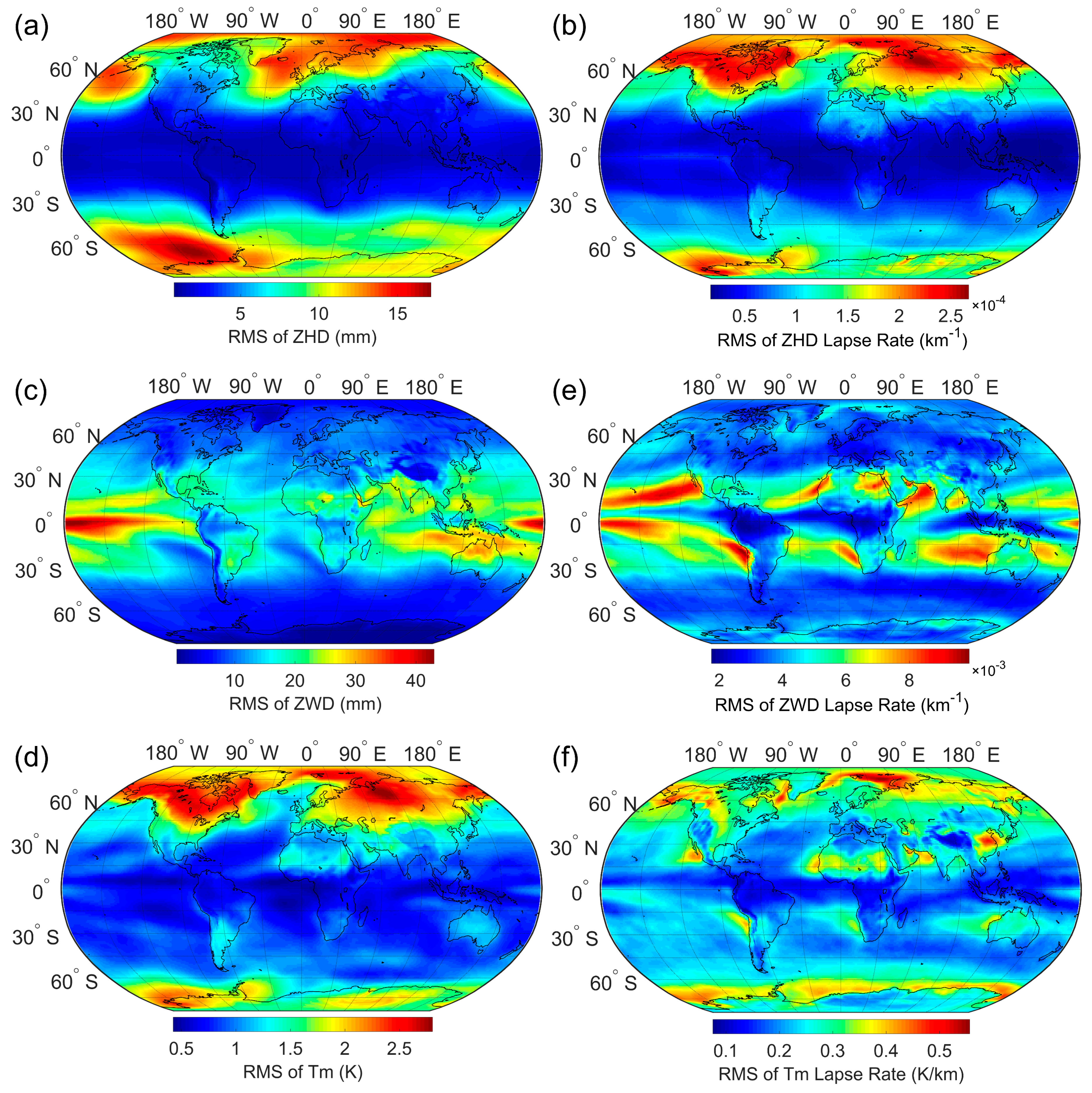
2.4. Height Corrections for Tropospheric Delay and T_m

To determine the method for height correction of tropospheric delay, we proposed two possible functions based on previous studies [8,9,10,11,36,37,38] and tested their accuracies. These two functions are expressed as:

$$\mathrm{TD}={\mathrm{TD}}_0·{e }^{-\alpha \left(h-h_0\right)}$$

(5)

$$\mathrm{TD}={\mathrm{TD}}_0·{\left[1-\alpha \left(h-h_0\right)\right]}^{5.225}$$

(6)

where TD indicates the tropospheric delay (ZHD or ZWD), TD₀ is the tropospheric delay (m) at the height of the grid point h₀ (km), h is the target height (km), and $\alpha$ denotes the lapse rate (km⁻¹) for tropospheric delay.

To test the height correction performances of Equations (5) and (6), we used them to fit the ECMWF-derived ZHD and ZWD profiles in June, 2017 at the same grid points selected in Section 2.3. The fitting results are shown in Figure 4 and Figure 5, respectively, and the root mean square (RMS) of the fitting residuals are summarized in

Table 2. Root mean square (RMS) of the fitting residuals in ZHD and ZWD profiles with Equations (5) and (6).

Fit Name	ZHD RMS (mm)				ZWD RMS (mm)
	0°N 115°E	30°N 115°E	60°N 115°E	90°N 115°E	0°N 115°E	30°N 115°E	60°N 115°E	90°N 115°E
Fit with Equation (5)	17.1	15.3	19.3	15.6	9.7	10.0	14.0	2.8
Fit with Equation (6)	1.6	3.6	0.7	3.6	6.2	5.4	1.2	1.5

.

Figure 4e–h shows that the ZHD fitting residuals from Equation (6) are overall smaller than those from Equation (5) at these four grid points. Figure 5e–h shows that the ZWD fitting residuals from Equation (6) are overall smaller than those from Equation (5) at the grid point 60°N and 115°E, and are similar at the other three grid points. Table 2 shows that the RMS of the fitting residuals from Equation (6) are all smaller than those from Equation (5). We also tested other grid points by fitting ZHD and ZWD profiles with Equations (5) and (6). The results also show that the RMS of the fitting residuals from Equation (6) are smaller than those from Equation (5). Therefore, we used Equation (6) in our new model as the height correction method for tropospheric delay.

As for T_m, we adopted the linear correction method that uses a linear lapse rate [24,26,28]:

$${\mathrm{T}}_{\mathrm{m}}={\mathrm{T}}_{\mathrm{m}0}-\beta \left(h-h_0\right)$$

(7)

where T_m0 is the weighted mean temperature (K) at the height of the grid point h₀ (km), and $\beta$ denotes the lapse rate (K/km) for T_m. This linear model for the height correction of T_m is justified by the almost constant vertical lapse rate, which is a result of the adiabatic expansion of air with elevation.

We used the ECMWF-derived ZHD, ZWD, and T_m profiles to invert for the lapse rate for ZHD (${\alpha }_{\mathrm{ZHD}}$), the lapse rate for ZWD (${\alpha }_{\mathrm{ZWD}}$), and the lapse rate for T_m $\left(\beta \right)$ by a least square method. We calculated the monthly values of these lapse rates from 1979 to 2017 and show two examples in Figure 6 to demonstrate that the lapse rates also have linear trends and seasonal variations. In Figure 6, we use straight lines to show the linear trends and use 4-term Fourier series with annual and semi-annual periods to describe the seasonal variations.

Figure 6 shows that the Fourier series agree well with the ${\alpha }_{\mathrm{ZHD}}{, \alpha }_{\mathrm{ZWD}}, \mathrm{and} \beta$, indicating the seasonal variations in lapse rates, which is modeled in our new model. To justify the significance of the linear trends in lapse rates, we performed significance tests and calculated the corresponding p values. The p values of the linear trends in ${\alpha }_{\mathrm{ZHD}}{, \alpha }_{\mathrm{ZWD},} \mathrm{and} \beta$ are 0.01, 8 × 10⁻³, and 5 × 10⁻⁴ at grid point 60°N and 115°E, and are 3 × 10⁻⁸, 9 × 10⁻⁸, and 3 × 10⁻⁷ at grid point 90°N and 115°E. All these p values are smaller than 0.05, indicating that the lapse rates at these two grid points have linear trends.

Then, we calculated the linear trends, their uncertainties at the 95% confidence level, the correlation coefficients, and the p values for the lapse rates at all the grid points, and present the results in Figures S2 and S3 of the SM. The statistics in Figure S3 show that 58.2% (38,058 of 65,341), 41.4% (27,076 of 65,341), and 48.4% (31,631 of 65,341) of the grid points have p values smaller than 0.05 for the lapse rates of ZHD, ZWD, and T_m, indicating that the linear trends in lapse rates at the corresponding grid points indeed exist.

2.5. Establishing a New Global Empirical Model

Previous studies have demonstrated that tropospheric delay and T_m have strong seasonal variations [10,21], and our study verified the linear trends. Therefore, in our new model, the temporal variations of ZHD, ZWD, and T_m are characterized by linear trends and seasonal variations (i.e., annual and semi-annual variations). The vertical variations of ZHD and ZWD are described by Equation (6) while the vertical variation of T_m is described by Equation (7). The temporal variations in their lapse rates are also characterized by linear trends and seasonal variations. Based on these assumptions, Equations (8) and (9) are proposed to model ZHD, ZWD, and T_m at a given point:

$$\begin{gathered} \mathrm{TD}=\left[A_1+A_2\left(Y-1980\right)+A_3\cos \left(\frac{\mathit{DOY}}{365.25}2\mathsf{\pi }\right)+A_4\sin \left(\frac{\mathit{DOY}}{365.25}2\mathsf{\pi }\right)+A_5\cos \left(\frac{\mathit{DOY}}{365.25}4\mathsf{\pi }\right)+A_6\sin \left(\frac{\mathit{DOY}}{365.25}4\mathsf{\pi }\right)\right]\times \\ {\left\{1-\left[A_7+A_8\left(Y-1980\right)+A_9\cos \left(\frac{\mathit{DOY}}{365.25}2\mathsf{\pi }\right)+A_{10}\sin \left(\frac{\mathit{DOY}}{365.25}2\mathsf{\pi }\right)+A_{11}\cos \left(\frac{\mathit{DOY}}{365.25}4\mathsf{\pi }\right)+A_{12}\sin \left(\frac{\mathit{DOY}}{365.25}4\mathsf{\pi }\right)\right]\left(h-h_0\right)\right\}}^{5.225} \end{gathered}$$

(8)

$$\begin{gathered} {\mathrm{T}}_{\mathrm{m}}=\left[B_1+B_2\left(Y-1980\right)+B_3\cos \left(\frac{\mathit{DOY}}{365.25}2\mathsf{\pi }\right)+B_4\sin \left(\frac{\mathit{DOY}}{365.25}2\mathsf{\pi }\right)+B_5\cos \left(\frac{\mathit{DOY}}{365.25}4\mathsf{\pi }\right)+B_6\sin \left(\frac{\mathit{DOY}}{365.25}4\mathsf{\pi }\right)\right]- \\ \left[B_7+B_8\left(Y-1980\right)+B_9\cos \left(\frac{\mathit{DOY}}{365.25}2\mathsf{\pi }\right)+B_{10}\sin \left(\frac{\mathit{DOY}}{365.25}2\mathsf{\pi }\right)+B_{11}\cos \left(\frac{\mathit{DOY}}{365.25}4\mathsf{\pi }\right)+B_{12}\sin \left(\frac{\mathit{DOY}}{365.25}4\mathsf{\pi }\right)\right]\left(h-h_0\right) \end{gathered}$$

(9)

where DOY denotes the day of year, Y represents the year, h₀ is the height of the grid point (km), and h is the target height (km), A_i and B_i (i = 1~12) are model coefficients to be determined.

The model coefficients are computed at 1° × 1° to account for spatial variations. When determining the model coefficients at a given grid point, the A_i and B_i (i = 7~12) are first determined by fitting the lapse rate time series from 1979 to 2017 for ZHD, ZWD, and T_m, respectively, by a least square method. Then the A_i and B_i (i = 1~6) are inverted with the computed ZHD, ZWD, and T_m at the height of the grid point. The model coefficients are solved at all grid points over the globe. We display these coefficients in Figures S4–S9 of the SM by showing the global linear trends, mean values, annual amplitudes, and semi-annual amplitudes of ZHD, ZWD, T_m, and their lapse rates. This new model is named as GTrop (Global Tropospheric Model).

When using this new model, only latitude, longitude, ellipsoid height, and a specific time (year and day of the year) are required. The model first finds the four grid points that are closest to the given location. The required parameters at these four points at the given height are then calculated through Equations (8) and (9). Finally, a bilinear interpolation is employed to interpolate the required parameters at the given location.

3. Results

3.1. Fitting Results of the Model

Figure 7 shows the RMS of the fitting residuals for ZHD, ZWD, T_m, and their lapse rates on a global scale. The mean values of the RMS for ZHD, ZHD lapse rate, ZWD, ZWD lapse rate, T_m, and T_m lapse rate are 7.1 mm, 1.1 × 10⁻⁴ km⁻¹, 11.6 mm, 4.2 × 10⁻³ km⁻¹, 1.3 K, and 0.26 K/km, respectively; the median values are 7.0 mm, 1.0 × 10⁻⁴ km⁻¹, 10.0 mm, 3.8 × 10⁻³ km⁻¹, 1.2 K, and 0.25 K/km, respectively. The mean values are close to the median values. Outliers can distort mean values while median values are insensitive to blunders, and we hence believe that there should be no large uncertainties in the fitting results.

The RMS of ZHD, ZWD, T_m, and their lapse rates are overall very small but show different geographical characteristics. Figure 7a shows that the RMS of ZHD are larger in high-latitude regions than in low-latitude regions. This is because that the seasonal variations of ZHD are larger in high latitudes, which is shown in Figure S4c,d of the SM. Larger seasonal variations bring more difficulties in modeling ZHD, and thus lead to larger RMS. Figure 7b shows that the RMS of ZHD lapse rate are larger in high-latitude regions than in low-latitude regions. This is caused by the larger seasonal variations of ZHD lapse rate in high latitudes, which is evident in Figure S5c,d of the SM.

Figure 7c shows that the RMS of ZWD in the low-latitude regions are larger than those in the high-latitude regions. This should be due to that the low-latitude regions are wetter than the high-latitude regions, which is evident by Figure S6b of the SM. The water vapor in low latitudes is abundant and highly changeable, which causes larger RMS there. Figure 7d shows that the RMS of ZWD lapse rate are larger in the low-latitude regions than in the high-latitude regions. This is due to that the magnitudes of the ZWD lapse rate are larger in low latitudes than in high latitudes, which can be observed from Figure S7b of the SM.

Figure 7e shows that the RMS of T_m are larger in high-latitude regions than in low-latitude regions. This is because that the seasonal variations of T_m are larger in high latitudes (see Figure S8c,d of the SM), which brings more difficulties in modeling T_m and thus lead to larger RMS. Figure 7f shows that the RMS of T_m lapse rate in high-latitude regions are larger than those in low-latitude regions. Figure S9c,d of the SM shows that the seasonal variations of T_m lapse rate are larger in high latitudes, which cause larger RMS there.

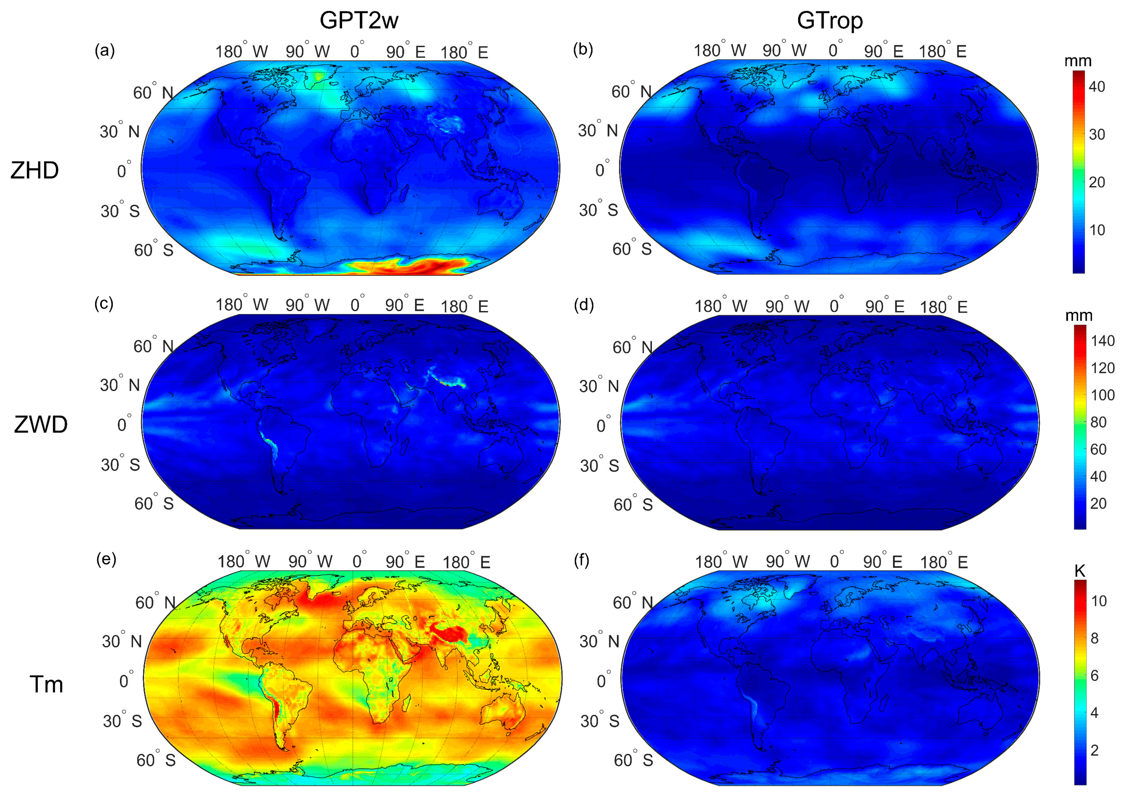
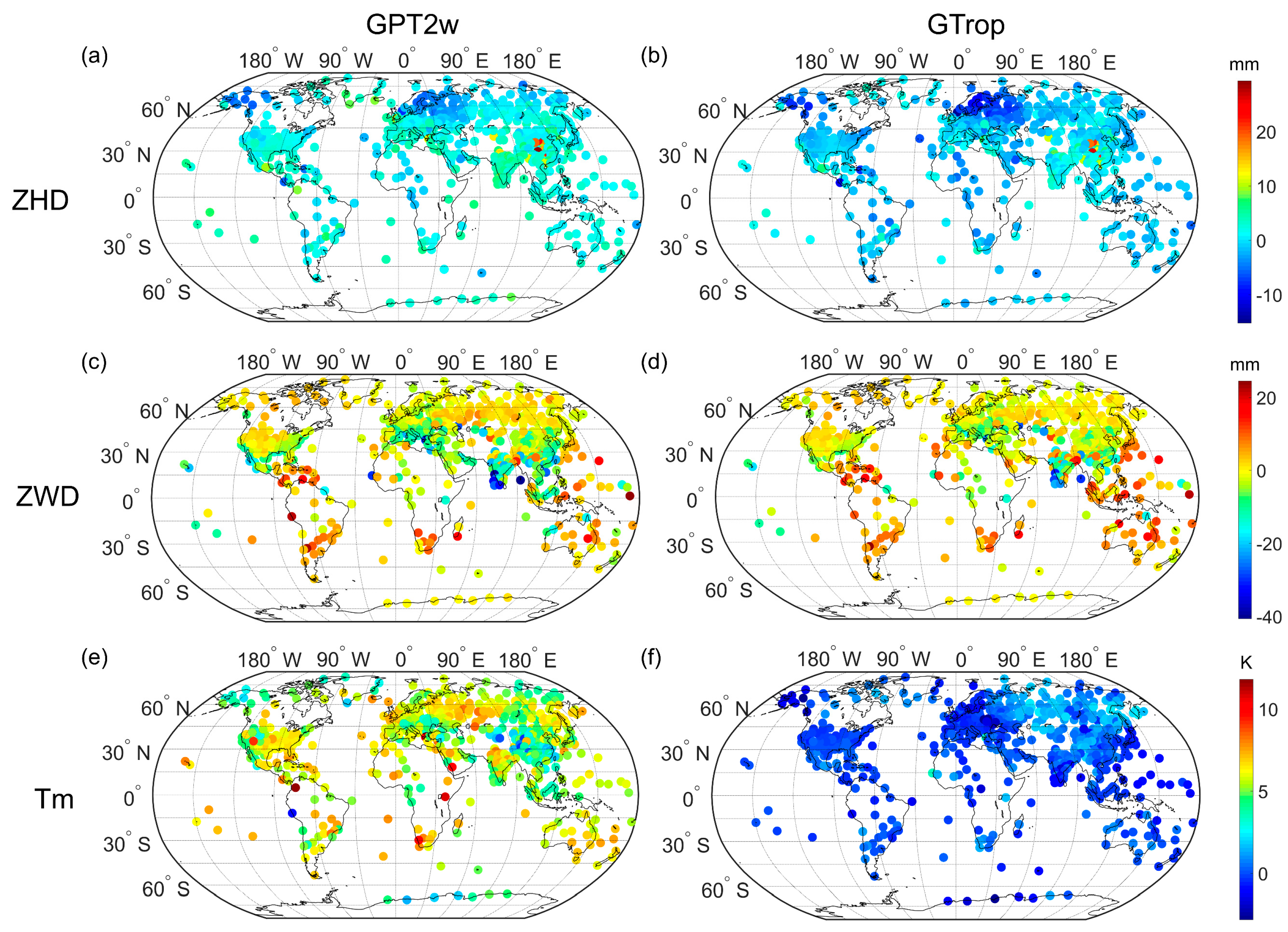
3.2. Validate the Model by European Centre for Medium-Range Weather Forecasts (ECMWF) Data

A new data set of ECMWF ERA-Interim monthly 1° × 1° data in 2018 is employed to validate the GTrop model. The canonical GPT2w model [11] is employed for comparison. In actual cases, the GNSS stations may be located below or above the nearby grid points, therefore vertical interpolation and extrapolation are required when using these two models. To test the model performance in severe height correction cases, we use the ECMWF data available at −3 km to 3 km height relative to the earth surface to do this validation. It should be noted that the ECMWF data are provided according to pressure levels from 1000 hPa to 1 hPa. At high-altitude regions, 1000 hPa corresponds to an ellipsoid height that is much lower than the earth surface, that’s why we can obtain data at -3 km height. We calculate ZHD, ZWD, T_m at all available pressure levels whose ellipsoid heights are at −3 km to 3 km relative to the earth surface by the two models and by the method represented by Equations (1)–(4). The latter results are treated as the reference values. Global biases of ZHD, ZWD, and T_m from the two models are presented in Figure 8, global RMS are presented in Figure 9, and the detailed statistical results are shown in

Table 3. Validation results of GPT2w and GTrop models tested by ECMWF ERA-Interim data and radiosonde data in 2018.

Validation Data	Model	ZHD		ZWD		Tm
		Bias (mm)	RMS (mm)	Bias (mm)	RMS (mm)	Bias (K)	RMS (K)
ECMWF Data	GPT2w	5.8 [−4.0, 29.3]	10.8 [1.7, 43.2]	0.4 [−32.2, 90.3]	10.5 [1.3, 151.2]	4.8 [−6.9, 8.3]	7.0 [3.7, 11.1]
	GTrop	1.0 [−6.9, 8.9]	6.5 [0.8, 16.3]	1.3 [−30.8, 23.3]	9.6 [0.4, 41.9]	−0.1 [−2.5, 3.3]	1.5 [0.1, 4.2]
Radiosonde Data	GPT2w	2.0 [−8.2, 29.3]	13.5 [4.4, 38.4]	−2.3 [−40.6, 24.2]	33.5 [6.1, 120.6]	5.4 [−0.7, 11.8]	8.5 [3.9, 14.7]
	GTrop	−0.9 [−15.2, 25.9]	12.3 [2.2, 39.7]	−0.4 [−30.5, 24.5]	33.1 [6.0, 120.2]	0.2 [−2.8, 3.5]	4.0 [1.3, 6.9]

.

Figure 8a shows that the GPT2w model mainly shows positive ZHD bias and has large positive bias in Antarctic and Greenland. According to Table 3, the averaged ZHD bias from the GPT2w model is 5.8 mm. Figure 8b shows that the GTrop model has small ZHD bias globally with a mean value of only 1.0 mm. This indicates that the GTrop model shows better bias than the GPT2w model in estimating ZHD, especially in Antarctic and Greenland. Figure 8e, f shows that the GPT2w model has obvious positive T_m bias with a mean value of 4.8 K, while the GTrop model has small T_m bias in most regions with a mean value of −0.1 K, indicating that the GTrop model has better bias than the GPT2w model in estimating T_m.

According to other studies [11,12,27], the biases in ZHD and T_m from the GPT2w model are near zero at the earth surface. However, in our study, we evaluate the model accuracy not only at the earth surface but also in the range of −3 km to 3 km height. The GPT2w model shows large bias in our validation, while the bias of the GTrop model is still small. This demonstrates that the GPT2w model can introduce large uncertainties to the tropospheric delay and T_m estimates when height difference between the reference height and the target height is large due to its insufficient height corrections, while the GTrop model can well handle this problem.

Figure 9a,b shows that the GPT2w model has larger ZHD RMS than the GTrop model in Antarctic, indicating that the GTrop model has higher accuracy than the GPT2w model in estimating ZHD in this region. Figure 9e,f shows that the GPT2w model has larger T_m RMS than the GTrop model over the globe, indicating that the GTrop model shows higher accuracy than the GPT2w model in estimating T_m globally.

3.3. Validation of the Model by Radiosonde Data

ZHD, ZWD, and T_m profiles derived from radiosonde measurements at globally distributed 586 stations in 2018 were used to validate the GPT2w and GTrop models. We also validate the model performance from the station height to 3 km height above it. Bias and RMS of ZHD, ZWD, and T_m at each station were computed and are presented in Figure 10 and Figure 11, respectively. Detailed statistical results are shown in Table 3.

Figure 10a shows that the GPT2w model has positive ZHD bias at most stations, and Table 3 shows that the averaged ZHD bias for the GPT2w model is 2.0 mm. This should be due to the low precision of the height correction for ZHD in the GPT2w model. Figure 10b shows that the ZHD biases from the GTrop model are better than those from the GPT2w model, and the averaged ZHD bias from the GTrop model is −0.9 mm. Figure 10e shows that the GPT2w model has positive T_m bias at most stations, and the mean value is 5.5 K. This is because the GPT2w model neglects the height correction for T_m. Figure 10f shows that the GTrop model has small T_m bias at most stations with a mean value of 0.2 K. This further demonstrates that the ZHD and T_m biases from the GTrop model are better than those from the GPT2w model.

Figure 11a–d shows that the RMS of ZHD and ZWD from the GPT2w and GTrop models are comparative and show latitudinal gradients, i.e., larger at high latitudes than at low latitudes for ZHD RMS and larger at low latitudes than at high latitudes for ZWD RMS. Figure 11e, f shows that the GPT2w model has larger T_m RMS than the GTrop model, which is consistent with the results shown in Figure 9. This further demonstrates that the GTrop model retains higher accuracy than the GPT2w model in estimating T_m.

Table 3 shows that the RMS from the GTrop model are overall smaller than those from the GPT2w model in all parameters. When validated by the ECMWF ERA-Interim data, the ZHD, ZWD, and T_m improvements are 39.8%, 8.6%, and 78.6%, respectively. When validated by the radiosonde data, these improvements become 9.0%, 1.2%, and 53.5%. We attribute these improvements to the modeling of linear trends and the advancement of height corrections in our new model.

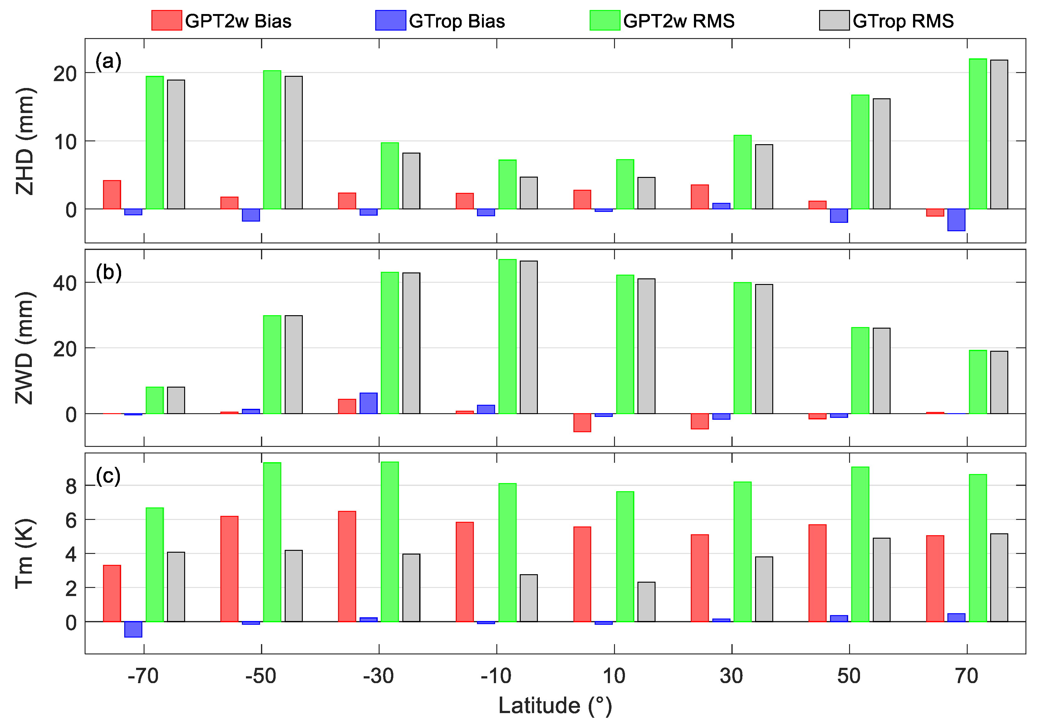
3.4. Latitudinal Variations of the Model Accuracy

To investigate the latitudinal variations of the model accuracy, we first divided the whole globe into eight bands along the latitudinal direction (20° sampling interval). The biases and RMS of ZHD, ZWD, and T_m from the GPT2w and GTrop models validated by the radiosonde data in 2018 were then computed and averaged within each latitudinal band. The statistical results are presented in Figure 12.

Figure 12a shows that the ZHD from the GPT2w model mainly have positive biases, while ZHD biases from the GTrop model are small. The ZHD RMS from the two models are both smaller at low-latitude bands and larger at high-latitude bands. This result is consistent with those shown in Figure 11a, b, which is mainly due to the fact that the seasonal variations of ZHD are larger at high latitudes than at low latitudes. The ZHD RMS from the GTrop model are smaller than those from the GPT2w model at all latitude bands. The improvements are larger at low latitudes. This indicates that the GTrop model improves the accuracy in estimating ZHD compared to the GPT2w model, especially in the low-latitude regions.

Figure 12b shows that the ZWD RMS from the GPT2w model and the GTrop model are both larger at low-latitude bands and smaller at high-latitude bands. This result is consistent with those shown in Figure 11c,d. This could be due to the fact that the low latitudes are wetter with highly dynamic water vapor than in the high latitudes. The ZWD RMS from the two models are comparable, indicating that these two models have similar accuracies in estimating ZWD over the globe.

Figure 12c shows that the GPT2w model has large positive T_m bias in all bands. This is because the GPT2w model neglects the height correction for T_m. However, the GTrop model has small and stable T_m bias. This could be due to the fact that the GTrop model considers the height correction for T_m and carefully models the T_m lapse rate by characterizing the temporal variation by linear trend, annual, and semi-annual variations. Therefore, the T_m RMS from the GTrop model are far smaller than those from the GPT2w model. This indicates that the GTrop model largely improves the accuracy in estimating T_m than the GPT2w model. It should be noted that the T_m RMS from the two models are larger at mid-latitudes than those at low- and high-latitudes.

3.5. Seasonal Variations of the Model Accuracy

To investigate the seasonal variations of the model accuracy, we calculated biases and RMS of ZHD, ZWD, and T_m from the GPT2w and GTrop models validated by the radiosonde data in 2018 in four seasons and present them in Figure 13. We calculated the biases and RMS for both the North Hemisphere (NH) and the South Hemisphere (SH) due to that the seasonal variations in these two hemispheres being different.

Figure 13a shows that in the NH, the ZHD RMS from the GPT2w and GTrop models are both larger in winter than in summer. This is because in the NH, the seasonal amplitudes of ZHD are larger in winter than in summer. The larger amplitudes bring more difficulties in modeling ZHD and result in larger RMS. Figure 13b shows that in the SH, the ZHD RMS from these two models are larger in summer than in winter. This is because the seasonal amplitudes of ZHD are larger in summer than in winter in the SH. The GTrop model has smaller ZHD RMS than the GPT2w model in all the four seasons and in both hemispheres. This indicates that the ZHD from the GTrop model have higher accuracy than those from the GPT2w model in the whole year and on a global scale.

Figure 13c shows that the two models both have larger ZWD RMS in summer than in winter in the NH, while Figure 13d shows that they have larger ZWD RMS in winter than in summer in the SH. This could be due to the fact that compared with summer, the winter is drier in the NH and wetter in the SH. The drier season leads to smaller variations in ZWD, which is beneficial for obtaining smaller RMS. The ZWD RMS from the two models are comparative, indicating that the GTrop model and the GPT2w model have the similar accuracy in estimating ZWD.

Figure 13e shows that the T_m RMS from the two models are larger in winter than in summer in the NH, while Figure 13f shows that the T_m RMS are larger in summer than in winter in the SH. This is because the seasonal amplitudes of T_m are larger in winter than in summer in the NH and larger in summer than in winter in the SH. The T_m RMS from the GPT2w model are larger than those from the GTrop model. This is because the GPT2w model has large positive T_m bias in all the four seasons, while those from the GTrop model are small. We attribute this to the fact that the GTrop model well models the lapse rate of T_m while the GPT2w model neglects it.

3.6. Vertical Variations of the Model Accuracy

To investigate the vertical variations of the model accuracy, we divided the height from 0 km to 10 km into ten layers (1 km sampling interval). Then we calculated biases and RMS of ZHD, ZWD, and T_m from the GPT2w and GTrop models validated by the radiosonde data in 2018 at different height layers and present them in Figure 14.

Figure 14a shows that the GPT2w model shows very large positive ZHD bias at high heights, while the ZHD biases from the GTrop model are still small at these heights. The ZHD RMS from the GPT2w model increases with increasing height and reaches ~80 mm at 10 km height, while ZHD RMS from the GTrop model stays at a low level at all heights and is only ~10 mm at 10 km height. This indicates that the GPT2w model has large uncertainties in estimating ZHD at high-altitude (relative to the reference height) regions, while the accuracies of the GTrop model stay at a high level at all heights.

Figure 14b shows that the ZWD biases from the two models are small at all heights. The ZWD RMS from them both decrease with increasing height. This is because the higher altitude is drier than the lower altitude. The drier atmosphere results in smaller variations in ZWD, which is beneficial for obtaining smaller RMS. The ZWD RMS from the two models are comparative, demonstrating that these two models have similar accuracies in estimating ZWD.

Figure 14c shows that the GPT2w model has large positive bias in estimating T_m at high altitudes. The T_m RMS from the GPT2w model increase with increasing height. The maximum RMS is ~50 K and occurred at 10 km height. However, the GTrop model has small and stable T_m RMS at all heights, and the RMS is ~4 K at 10 km. We attribute this to the fact that the GPT2w model does not take the height correction for T_m into account while the GTrop model well considers the height correction.

4. Discussion

The validation by the radiosonde data is limited by the fact that radiosonde stations are not evenly distributed on the earth, i.e., most on land, a few on islands, more in the Northern Hemisphere than in the Southern Hemisphere. To compensate for this, we used the ECMWF ERA-Interim data in 2018 to validate the two models. The ECMWF ERA-Interim data are evenly distributed in the globe with a spatial resolution of 1° × 1°. In addition, we employed radiosonde data collected from 586 stations in 2018 to validate these two models. Some of the radiosonde stations are located in the South Hemisphere (see Figure 1). Therefore, the validation results should be valid around the globe. The validation results indicate that our new model GTrop outperforms the canonical GPT2w model. The performance improvements are mainly attributed to two improved parts in the GTrop model.

The first improved part is that the GTrop model employs model data covering a period as long as ~40 years. This long time span guarantees that the linear trends can be detected and modeled. The linear trend is a first-order approximation of the complex atmospheric variations. For tropospheric parameters, their seasonal variations are much stronger than the linear trends, and thus only modeling seasonal variations can account for most of the temporal variations. However, according to our studies, we find that the ZHD, ZWD, T_m, and their lapse rates indeed have linear trends in some regions, which has passed the significance tests. Therefore, we assume that the model performance can be further improved by considering the linear trends in modeling. To investigate how much improvement can be achieved with this new consideration, we calculated the improvements of the fitting results compared with the results without considering linear trends and present them in Figure S10 of the SM. It shows that the improvements can reach 10%–30% in some regions (these regions are typically the regions with strong linear correlation, which can be observed from Figures S1a,c,e and S3a,c,e of the SM).

The second improved part is the height correction of the GTrop model. Previous studies usually address model accuracies at or near the reference heights without spending more efforts on height corrections. Since the GNSS stations are usually not located at or near the reference heights, proper height corrections are therefore required. The GTrop model carefully models the vertical variations of tropospheric delay and T_m by modeling their lapse rates, and consequently advances the performance of height correction.

The GTrop model demonstrates to be superior to the GPT2w model. This superiority in model accuracy can be theoretically propagated to the PWV estimates. Literature study [39] gives the mathematical relationship between the uncertainties of T_m and ZWD and the uncertainties of PWV. It shows that the PWV uncertainties rely on the uncertainties of T_m and ZWD. In addition, the positioning accuracies can also benefit from the improved ZHD accuracies [5]. The applications in GNSS meteorology and positioning with the GTrop model will be left for a future study.

5. Conclusions

In this study, we used ECMWF ERA-Interim data from 1979 to 2017 to investigate the temporal variations of ZHD, ZWD, and T_m and demonstrated that they all have linear trends besides the seasonal variations. Then, we tested the accuracies of two possible functions for the height corrections of tropospheric delay, and determined the optimal one. Based on these findings, we built a new model that considers the linear trends and seasonal variations in ZHD, ZWD, T_m, and their lapse rates. This new model can provide ZHD, ZWD, and T_m worldwide with the spatial resolution of 1° × 1°. Validation results demonstrate that this new model shows higher accuracy than the canonical GPT2w model in all parameters. The improvements are 39.8%, 8.6%, and 78.6% for ZHD, ZWD, and T_m in terms of RMS when validated by the ECMWF ERA- Interim data in 2018, and are 9.0%, 1.2%, and 53.5% when validated by the radiosonde data in 2018. This model especially improves the accuracies in ZHD and T_m at high-altitude (relative to the grid point height) regions. This new model integrates tropospheric delay correction and T_m calculation and thus contributes to GNSS-based real-time PWV retrieval and also benefits GNSS positioning. The MATLAB source code of this new model is available at https://github.com/sun1753814280/GTrop.

References

1. Leick, A. GPS satellite surveying. J. Geol. 1990, 22, 181–182. [Google Scholar]
2. Davis, J.L.; Herring, T.A.; Shapiro, I.I.; Rogers, A.E.E.; Elgered, G. Geodesy by radio interferometry: Effects of atmospheric modeling errors on estimates of baseline length. Radio Sci. 1985, 20, 1593–1607. [Google Scholar] [CrossRef]
3. Askne, J.; Nordius, H. Estimation of Tropospheric Delay for Mircowaves from Surface Weather Data. Radio Sci. 1987, 22, 379–386. [Google Scholar] [CrossRef]
4. Ifadis, I.M. Space to earth techniques: Some considerations on the zenith wet path delay parameters. Surv. Rev. 1993, 32, 130–144. [Google Scholar] [CrossRef]
5. Tregoning, P.; Herring, T.A. Impact of a priori zenith hydrostatic delay errors on GPS estimates of station heights and zenith total delays. Geophys. Res. Lett. 2006, 33, 33. [Google Scholar] [CrossRef]
6. Saastamoinen, J. Atmospheric correction for the troposphere and stratosphere in radio ranging satellites. Geophys. Monogr. Ser. 1972, 15, 247–251. [Google Scholar]
7. Hopfield, H.S. Tropospheric effect on electromagnetically measured range: Prediction from surface weather data. Radio Sci. 1971, 6, 357–367. [Google Scholar] [CrossRef]
8. Leandro, R.F.; Langley, R.B.; Santos, M.C. UNB3m_pack: A neutral atmosphere delay package for radiometric space techniques. GPS Solut. 2008, 12, 65–70. [Google Scholar] [CrossRef]
9. Schüler, T. The TropGrid2 standard tropospheric correction model. GPS Solut. 2014, 18, 123–131. [Google Scholar] [CrossRef]
10. Böhm, J.; Heinkelmann, R.; Schuh, H. Short note: A global model of pressure and temperature for geodetic applications. J. Geod. 2007, 81, 679–683. [Google Scholar] [CrossRef]
11. Böhm, J.; Möller, G.; Schindelegger, M.; Pain, G.; Weber, R. Development of an improved empirical model for slant delays in then troposphere (GPT2w). GPS Solut. 2015, 19, 433–441. [Google Scholar] [CrossRef]
12. Yao, Y.; Xu, C.; Shi, J.; Cao, N.; Zhang, B.; Yang, J. ITG: A new global GNSS tropospheric correction model. Sci. Rep. 2015, 5, 10273. [Google Scholar] [CrossRef] [PubMed]
13. Lagler, K.; Schindelegger, M.; Böhm, J.; Krásná, H.; Nilsson, T. GPT2: Empirical slant delay model for radio space geodetic techniques. Geophys. Res. Lett. 2013, 40, 1069–1073. [Google Scholar] [CrossRef] [PubMed] [Green Version]
14. Landskron, D.; Böhm, J. VMF3/GPT3: Refined discrete and empirical troposphere mapping functions. J. Geod. 2018, 92, 349–360. [Google Scholar] [CrossRef] [PubMed]
15. Zhou, C.; Peng, B.; Li, W.; Zhong, S.; Ou, J.; Chen, R.; Zhao, X. Establishment of a Site-Specific Tropospheric Model Based on Ground Meteorological Parameters over the China Region. Sensors 2017, 17, 1722. [Google Scholar] [CrossRef] [PubMed]
16. Yao, Y.; Hu, Y.; Yu, C.; Zhang, B.; Guo, J. An improved global zenith tropospheric delay model GZTD2 considering diurnal variations. Nonlinear Process. Geophys. 2016, 23, 127–136. [Google Scholar] [CrossRef] [Green Version]
17. Li, W.; Yuan, Y.; Ou, J.; Chai, Y.; Li, Z.; Liou, Y.; Wang, N. New versions of the BDS/GNSS zenith tropospheric delay model IGGtrop. J. Geod. 2015, 89, 73–80. [Google Scholar] [CrossRef]
18. Li, W.; Yuan, Y.; Ou, J.; He, Y. IGGtrop_SH and IGGtrop_rH: Two Improved Empirical Tropospheric Delay Models Based on Vertical Reduction Functions. IEEE Trans. Geosci. Remote Sens. 2018, 56, 5276–5288. [Google Scholar] [CrossRef]
19. Bevis, M.; Businger, S.; Herring, T.A.; Rocken, C.; Anthes, R.A.; Ware, R.H. GPS meteorology: Remote sensing of atmospheric water vapor using the global positioning system. J. Geophys. Res. Atmos. 1992, 97, 15787–15801. [Google Scholar] [CrossRef]
20. Bevis, M.; Businger, S.; Chiswell, S.; Herring, T.A.; Anthes, R.A.; Rocken, C.; Ware, R.H. GPS meteorology: Mapping zenith wet delays onto precipitable water. J. Appl. Meteorol. Clim. 1994, 33, 379–386. [Google Scholar] [CrossRef]
21. Yao, Y.; Zhu, S.; Yue, S. A globally applicable, season-specific model for estimating the weighted mean temperature of the atmosphere. J. Geod. 2012, 86, 1125–1135. [Google Scholar] [CrossRef]
22. Chen, P.; Yao, W.; Zhu, X. Realization of global empirical model for mapping zenith wet delays onto precipitable water using NCEP re-analysis data. Geophys. J. Int. 2014, 198, 1748–1757. [Google Scholar] [CrossRef] [Green Version]
23. He, C.; Wu, S.; Wang, X.; Hu, A.; Wang, Q.; Zhang, K. A new voxel-based model for the determination of atmospheric weighted mean temperature in GPS atmospheric sounding. Atmos. Meas. Tech. 2017, 10, 2045–2060. [Google Scholar] [CrossRef] [Green Version]
24. Zhang, H.; Yuan, Y.; Li, W.; Ou, J.; Li, Y.; Zhang, B. GPS PPP derived precipitable water vapor retrieval based on Tm/Ps from multiple sources of meteorological data sets in China. J. Geophys. Res. Atmos. 2017, 122, 4165–4183. [Google Scholar] [CrossRef]
25. Ding, M. A neural network model for predicting weighted mean temperature. J. Geod. 2018, 92, 1187–1198. [Google Scholar] [CrossRef]
26. Yao, Y.; Sun, Z.; Xu, C.; Xu, X.; Kong, J. Extending a model for water vapor sounding by ground-based GNSS in the vertical direction. J. Atmos. Sol. Terr. Phys. 2018, 179, 358–366. [Google Scholar] [CrossRef]
27. Huang, L.; Jiang, W.; Liu, L.; Chen, H.; Ye, S. A new global grid model for the determination of atmospheric weighted mean temperature in GPS precipitable water vapor. J. Geod. 2018, 93, 159–176. [Google Scholar] [CrossRef]
28. Huang, L.; Liu, L.; Chen, H.; Jiang, W. An improved atmospheric weighted mean temperature model and its impact on GNSS precipitable water vapor estimates for China. GPS Solut. 2019, 23, 51. [Google Scholar] [CrossRef]
29. Wang, X.; Zhang, K.; Wu, S.; Fan, S.; Cheng, Y. Water vapor weighted mean temperature and its impact on the determination of precipitable water vapor and its linear trend. J. Geophys. Res. Atmos. 2016, 121, 833–852. [Google Scholar] [CrossRef]
30. Chen, B.; Liu, Z. Global water vapor variability and trend from the latest 36 year (1979 to 2014) data of ECMWF and NCEP reanalyses, radiosonde, GPS, and microwave satellite. J. Geophys. Res. Atmos. 2016, 121, 11–442. [Google Scholar] [CrossRef]
31. Wang, X.; Zhang, K.; Wu, S.; Li, Z.; Cheng, Y.; Li, L.; Yuan, H. The correlation between GNSS-derived precipitable water vapor and sea surface temperature and its responses to El Niño–Southern Oscillation. Remote Sens. Environ. 2018, 216, 1–12. [Google Scholar] [CrossRef]
32. Simmons, A.; Uppala, D.; Kobayashi, S. ERA-Interim: New ECMWF reanalysis products from 1989 onwards. ECMWF Newsl. 2007, 110, 25–35. [Google Scholar]
33. Dee, D.; Uppala, S.; Simmons, A.; Berrisford, P.; Poli, P.; Kobayashi, S.; Andrae, U.; Balmaseda, M.; Balsamo, G.; Bauer, P. The ERA-Interim reanalysis: Configuration and performance of the data assimilation system. Q. J. R. Meteorol. Soc. 2011, 137, 553–597. [Google Scholar] [CrossRef]
34. Chen, B.; Liu, Z. A comprehensive evaluation and analysis of the performance of multiple tropospheric models in China region. IEEE Trans. Geosci. Remote Sens. 2015, 54, 663–678. [Google Scholar] [CrossRef]
35. Rüeger, J.M. Refractive Index Formulae for Radio Waves. JS28 Integration of Techniques and Corrections to Achieve Accurate Engineering; FIG XXII International Congress: Washington, DC, USA, 2002. [Google Scholar]
36. Dousa, J.; Elias, M. An improved model for calculating tropospheric wet delay. Geophys. Res. Lett. 2014, 41, 4389–4397. [Google Scholar] [CrossRef]
37. Yao, Y.; Sun, Z.; Xu, C. Establishment and Evaluation of a New Meteorological Observation-Based Grid Model for Estimating Zenith Wet Delay in Ground-Based Global Navigation Satellite System (GNSS). Remote Sens. 2018, 10, 1718. [Google Scholar] [CrossRef]
38. Yao, Y.; Sun, Z.; Xu, C.; Zhang, L.; Wan, Y. Development and Assessment of the Atmospheric Pressure Vertical Correction Model with ERA Interim and Radiosonde Data. Earth Space Sci. 2018, 5, 777–789. [Google Scholar] [CrossRef]
39. Yao, Y.; Zhang, B.; Xu, C.; Yan, F. Improved one/multi-parameter models that consider seasonal and geographic variations for estimating weighted mean temperature in ground-based GPS meteorology. J. Geod. 2014, 88, 273–282. [Google Scholar] [CrossRef]
Figure 1. Global distribution of 586 selected radiosonde stations.
Remotesensing 11 01893 g001
Figure 2. Yearly zenith hydrostatic delay (ZHD), zenith wet delay (ZWD), and weighted mean temperature (Tm) from 1979 to 2017 and their linear trends at four grid points. (ad): blue dots are yearly ZHD and red lines are linear fit to them. (eh): purple dots are yearly ZWD and red lines are linear fit to them. (il): green dots are yearly Tm and red lines are linear fit to them.
Remotesensing 11 01893 g002
Figure 3. Linear trends and corresponding uncertainties at the 95% confidence level for ZHD (ab), ZWD (cd), and Tm (ef) derived from European Centre for Medium-Range Weather Forecasts (ECMWF) ERA- Interim data from 1979 to 2017.
Remotesensing 11 01893 g003
Figure 4. (ad): ZHD profiles at four grid points in June, 2017. (eh): Fitting residuals of the two fits.
Remotesensing 11 01893 g004
Figure 5. (ad): ZWD profiles at four grid points in June, 2017. (eh): Fitting residuals of the two fits.
Remotesensing 11 01893 g005
Figure 6. Time series of lapse rate for ZHD ( α ZHD ) (ab), lapse rate for ZWD ( α ZWD ) (cd), and lapse rate for Tm ( β ) (ef) from 1979 to 2017 at two grid points. Red lines indicate the linear trends, and the red curves are the 4-term Fourier series fitted to the α ZHD ,   α ZWD ,   and   β .
Remotesensing 11 01893 g006
Figure 7. Root mean square (RMS) of fitting residuals for ZHD (a), ZHD lapse rate (b), ZWD (c), ZWD lapse rate (d), Tm (e), and Tm lapse rate (f).
Remotesensing 11 01893 g007
Figure 8. Global biases of the ZHD (ab), ZWD (cd), and Tm (ef) for the GPT2w and GTrop models validated by ECMWF ERA-Interim monthly 1° × 1° data in 2018. The positive bias means the model output are larger than the reference values, while the negative bias means they are smaller than the reference values.
Remotesensing 11 01893 g008
Figure 9. Global RMS of the ZHD (ab), ZWD (cd), and Tm (ef) for the GPT2w and GTrop models validated by ECMWF ERA-Interim monthly 1° × 1° data in 2018.
Remotesensing 11 01893 g009
Figure 10. Biases of the ZHD (ab), ZWD (cd), and Tm (ef) for the GPT2w and GTrop models validated by radiosonde data in 2018. The positive bias means the model output are larger than the reference values, while the negative bias means they are smaller than the reference values.
Remotesensing 11 01893 g010
Figure 11. RMS of the ZHD (ab), ZWD (cd), and Tm (ef) for the GPT2w and GTrop models validated by radiosonde data in 2018.
Remotesensing 11 01893 g011
Figure 12. Biases and RMS of ZHD (a), ZWD (b), and Tm (c) for the GPT2w and GTrop models at different latitude bands validated by radiosonde data in 2018.
Remotesensing 11 01893 g012
Figure 13. Biases and RMS of ZHD (ab), ZWD (cd), and Tm (ef) for the GPT2w and GTrop models in four seasons and in two hemispheres validated by radiosonde data in 2018.
Remotesensing 11 01893 g013
Figure 14. Biases and RMS of ZHD (a), ZWD (b), and Tm (c) for the GPT2w and GTrop models at different heights validated by radiosonde data in 2018.
Remotesensing 11 01893 g014