Evaluating the Temperature Difference Parameter in the SSEBop Model with Satellite-Observed Land Surface Temperature Data

Abstract

The Operational Simplified Surface Energy Balance (SSEBop) model uses the principle of satellite psychrometry to produce spatially explicit actual evapotranspiration (ETa) with remotely sensed and weather data. The temperature difference (dT) in the model is a predefined parameter quantifying the difference between surface temperature at bare soil and air temperature at canopy level. Because dT is derived from the average-sky net radiation based primarily on climate data, validation of the dT estimation is critical for assuring a high-quality ETa product. We used the Moderate Resolution Imaging Spectroradiometer (MODIS) data to evaluate the SSEBop dT estimation for the conterminous United States. MODIS data (2008–2017) were processed to compute the 10-year average land surface temperature (LST) and normalized difference vegetation index (NDVI) at 1 km resolution and 8-day interval. The observed dT (dT_o) was computed from the LST difference between hot (NDVI < 0.25) and cold (NDVI > 0.7) pixels within each 2° × 2° sampling block. There were enough hot and cold pixels within each block to create dT_o timeseries in the West Coast and South-Central regions. The comparison of dT_o and modeled dT (dT_m) showed high agreement, with a bias of 0.8 K and a correlation coefficient of 0.88 on average. This study concludes that the dT_m estimation from the SSEBop model is reliable, which further assures the accuracy of the ETa estimation.

1. Introduction

As a process of transferring moisture from the land surface into the atmosphere, evapotranspiration (ET) is an important element in the hydrologic cycle of the Earth. Measurement and estimation of ET are essential and important for investigations and applications in hydrology, ecology, climatology, agriculture, and water resources management. However, accurate estimation of ET remains a challenge because ET is driven by numerous complexed factors including radiation, vapor-pressure deficit, temperature, soil moisture, and plant stomatal conductance [1,2,3,4]. Although direct ET measurement can be implemented using water budget methods (e.g., lysimeter, soil moisture depletion, and field experiment plot) and water vapor transfer methods (e.g., Bowen ratio energy budget and eddy covariance), the scale of the ET measurement is ground-based. Spatially explicit estimation of ET over a basin or a region relies on models that integrate ground information and atmospheric observations with remotely sensed data. Satellite remote sensing techniques have become increasingly attractive because they provide spatially and temporally contiguous observations from visible, infrared, and thermal infrared wavelengths for retrieving land surface parameters used for the energy balance and ET modeling.

Since the 1990s, various remote-sensing-based ET estimation models have been developed for estimating actual ET (ETa) using the surface energy balance method. Those well-known models include Surface Energy Balance Index (SEBI) [5], Two-Source Energy Balance (TSEB) [6], Surface Energy Balance Algorithm for Land (SEBAL) [7,8], Simplified Surface Energy Balance Index (S-SEBI) [9], Surface Energy Balance System (SEBS) [10], Mapping Evapotranspiration at high Resolution with Internalized Calibration (METRIC) [11,12], and Operational Simplified Surface Energy Balance (SSEBop) [13,14]. Some ET models are designed with high complexity to approximate the actual hydrological mechanisms and processes for increasing model accuracy, which require more input data and measurements to calibrate parameters. However, the complexity may influence the accuracy of the model output due to the potential errors in the input data and parameters. High requirement for input data also usually impedes the applications of ET estimation at regional or national scale. Other models have simplified structures, which eliminate less important processes in computation. Although these models may sacrifice accuracy to some extent, the simplicity benefits the model in operational applications over a large area.

The Simplified Surface Energy Balance (SSEB) method developed by Senay et al. 2007 [15] is a simplified thermal-based surface energy model. The model requires setting up uniform hydro-climatic regions where climatic conditions are comparable for the hot and cold reference pixels to limit the impact of confounding factors that cause changes in land surface temperature (LST). The SSEB formulation was enhanced by Senay et al. 2011a [16] to handle the impact of topography on surface temperature using a lapse rate correction factor. Later, Senay et al. 2011b [17] introduced a revised SSEB that handles both elevation and latitude effect on surface temperature using the difference between LST and air temperature. Furthermore, the SSEB was parameterized for operational applications and renamed to SSEBop (Operational SSEB) by Senay et al. 2013 [13]. The SSEBop model is formulated based on the principle of satellite psychrometry, which uses LST measured from satellite sensors to estimate the psychrometric surface equivalents of dry-bulb and wet-bulb air temperatures to calculate ET fractions and ETa for every pixel in an image. The SSEBop model uses predefined hot and cold reference boundary limits for each location and time, so that the estimation of ET fractions can be operationally implemented using the SSEB approach [13]. SSEBop is one of the simplest surface energy balance models for large-scale operational ET estimation because the model directly solves for latent heat flux without the need to solve for other surface energy balance components such as net radiation, sensible heat, and ground heat fluxes [13,14].

To meet the needs for water resource use and management, the U.S. Geological Survey (USGS) Earth Resources Observation and Science (EROS) Center routinely produces historical and near-real time ETa maps at regional, national, and global level using the SSEBop model. Those ETa products include (1) global 1 km ETa and ETa anomaly (ratio of concurrent ETa to long-term median value) maps (2003 to present) at dekadal (10-day), monthly, and yearly intervals [18], (2) nationwide 1 km ETa and ETa anomaly maps for the conterminous United States (CONUS) (2001 to present) at 8-day, and monthly, and yearly intervals [18], and (3) monthly and yearly 30 m ETa maps for some focus areas such as the Upper Rio Grande Basin [18] and the southwestern CONUS [19].

The SSEBop ETa products have been comprehensively validated at field scale using in situ flux tower data and at basin scale using water balance approaches. Comparisons of the SSEBop ETa against flux tower data were found to show reasonable accuracies across different landscapes [13,14,20,21,22,23]. For example, validation of the 1 km SSEBop ETa product with individual flux towers had R² of 0.70–0.97 across the CONUS [13]. Validation of the 100 m SSEBop ETa estimates in the Colorado River Basin using eddy covariance flux towers showed good accuracy levels with R² ranging from 0.74 to 0.95 [14]. Validations of the SSEBop ETa data at basin scale were also found to be reliable in previous studies [14,20,21] and comparable with other existing global ET datasets, such as the MOD16 ET [24,25] and the FLUXNET upscaling ET obtained by combining global flux tower records and machine-learning algorithm [26]. Furthermore, the SSEBop ETa product was found to be reliable in multi-model comparison studies across various landscapes and regions [27,28,29,30,31]. Although previous studies indicated a certain level of uncertainties of SSEBop ETa data in point scale in some locations, the data were more accurate at basin scale with uncertainties as low as 15–20% [22].

The SSEBop model computes ETa as a product of ET fraction generated from LST and reference ET using two key parameters, i.e., air temperature (T_a) for establishing a maximum ET limit condition (cold boundary) and predefined temperature difference (dT) between dry bare surface and canopy surface [13]. In the SSEBop model, dT is calculated from the surface energy balance equation under average-sky conditions for dry bare soil where ET is assumed to be zero, and sensible heat is assumed to be maximum [13,14]. Thus, dT is determined based on the assumption that the difference between the hot and cold values remains nearly constant from year-to-year for a given location and period under average-sky conditions [13,21]. Because dT is a key parameter in the SSEBop model, validation of the dT estimation is critical for assuring the accuracy of the ETa products. dT represents the LST difference between dry/hot bare soil pixels and wet/cold vegetated field pixels (assumed to be equal to canopy level air temperature). Direct validation of dT data would be impractical from field measurements because of the difficulty in obtaining air temperatures of dry/hot soil and wet/cold canopy at the same location, especially across a large ET mapping area. However, observations from satellite sensors provide a convenient and flexible tool for measuring LST for dry/hot and wet/cold pixels, which can be used to estimate dT and compare it with the modeled dT.

The objective of this study was to evaluate the SSEBop dT estimates using satellite LST observations. We collected and analyzed the Moderate Resolution Imaging Spectroradiometer (MODIS) surface reflectance data (2008–2017) to determine hot and cold pixels based on the normalized difference vegetation index (NDVI). We used the MODIS LST data to compute actual LST for hot and cold pixels to simulate observed dT, which was further compared with the dT data generated from the SSEBop model. We performed the evaluation of the dT products for sampling blocks across the CONUS. The degree of agreement between the satellite-observed dT and modeled dT was quantified to understand the accuracy of the SSEBop ET products.

As mentioned above, validations of the SSEBop estimates have been conducted through using flux tower data, flux tower-based gridded ETa estimates, and basin-scale water balance data [20,21,22,23] and through comparison with existing well-established ETa model estimates [27,28,29,30,31]. Although flux towers provide direct ETa measurements, the limited number of tower locations in space hampers wide and comprehensive use of the data for the model validation. Other gridded ETa products, either estimated from remote sensing-based models or from flux tower upscaling algorithms, are useful for evaluating the SSEBop product at pixel level. These modeled ETa products can be utilized for ETa data evaluation through cross-model or cross-data comparisons, but they cannot be referred to as the ground-observed references in the data validation. Unlike the ETa estimates, the dT parameter generated from the SSEBop model can be directly compared with satellite-observed LST at pixel level. Because MODIS contains abundant collections of LST and other land surface products, we choose to validate the dT data instead of the ETa data in this study. This method provides an auxiliary approach for evaluating the SSEBop model in addition to the previous model validation investigations [20,21,22,23,27,28,29,30,31].

2. Materials

2.1. Study Area

Our study area encompasses the CONUS with a map extent of 24–50°N and 66–126°W (Figure 1). The topography of the CONUS is featured by moderate elevations consisting of hills and low mountains in the east, low elevations in the vast central plains (i.e., the Great Plains), and high elevations with high rugged mountain ranges in the west. According to MODIS land cover data (MCD12Q1) [32], the primary classes of vegetated land in the CONUS are cropland (19.8%), forest (15.6%), shrubland and savanna (25.7%), grassland (34.3%), and wetland (0.6%). Based on the 30-year (1981–2010) climatology data [33], the annual average air temperature is 11.6 °C and total precipitation is 780 mm, calculated as the spatial means across the CONUS. The climate varies greatly, ranging from humid-subtropical in the Southeast, humid-continental in the Northeast and Midwest, semiarid in the western Great Plains, arid in the southwestern deserts, to Mediterranean along the western coast.

2.2. MODIS Data

We used a suite of MODIS datasets (Collection 6) including Land Surface Reflectance, Land Surface Temperature, Active Fire, and Land Cover to compute the observed dT parameter (

Table 1. MODIS datasets used for developing observed temperature difference (dT).

Product	Satellite	Attribute	Pixel Size	Compositing Interval	Output Dataset
MYD09A1	Aqua	Land surface reflectance	500 m	8-day	NDVI; cloud, cloud shadow, cirrus, and snow/ice masks
MYD11A2	Aqua	Land surface temperature	1 km	8-day	Land surface temperature
MYD14A2	Aqua	Active fire	1 km	8-day	Fire mask
MCD12Q1	Terra/Aqua combined	Land cover type	500 m	Annual	Vegetation cover

). All the MODIS datasets were obtained from the Application for Extracting and Exploring Analysis Ready Samples (AppEEARS) managed by the Land Processes Distributed Active Archive Center (LP DAAC) [34]. We downloaded the MODIS data for the CONUS map extent in the geographic coordinate system. The data included 1850 images of four MODIS products for the years from 2008 to 2017 (Table 1).

The Aqua MODIS Surface Reflectance is the MYD09A1 level-3 product containing surface reflectance at 500 m resolution for bands 1 (620–670 nm), 2 (841–876 nm), 3 (459–479 nm), 4 (545–565 nm), 5 (1230–1250 nm), 6 (1628–1652 nm), and 7 (2105–2155 nm). The dataset is an 8-day composite, with each pixel containing the best possible observation selected based on high observation coverage, low view angle, and absence of clouds, cloud shadow, or aerosol during an 8-day period. We used the MYD09A1 State Quality Assurance (QA) layer to extract cloud, cloud shadow, cirrus, and snow/ice data for each 8-day composite.

The Aqua MODIS Land Surface Temperature is the MYD11A2 level-3 product that provides 8-day composites of LST and emissivity at 1 km resolution. Each pixel value in the data is a simple average of all LST observed within the 8-day period. The daytime LST in Kelvin degree was extracted for this study.

The MODIS Active Fire is the MYD14A2 level-3 product at 8-day interval and 1 km resolution. The 8-day composite contains fire pixels detected in each pixel during the 8-day period. The Fire Mask layer in the MYD14A2 includes three categories of confidence levels: Low confidence, nominal confidence, and high confidence. We used the nominal and high confidence levels to identify the active fire pixels.

The Aqua MCD12Q1 (Collection 6) product provides the Terra and Aqua combined yearly land cover type at 500 m resolution. We used the International Geosphere-Biosphere Programme (IGBP) classification scheme, or Land Cover Type 1 in the MCD12Q1 data to identify vegetation cover. The vegetation cover includes evergreen forest, deciduous forest, mixed forest, closed shrubland, open shrubland, woody savanna, savanna, permanent wetland, cropland, and cropland/natural vegetation mosaics, while excluding urban and built-up land, permanent snow and ice, barren, and water bodies.

2.3. Modeled dT Data

In the SSEBop model, dT is an intermediate product derived from the surface energy balance equation [13]:

dT = (Rn × r_ah)/(p_a × C_p)

(1)

where Rn is the net radiation, r_ah is the aerodynamic resistance to heat transfer, p_a is the air density, and C_p is the specific heat of air. The most important assumption of the model is that the surface energy balance process is mostly driven by available net radiation, and a decline in ET due to water stress and other factors can be quantified by differences in LST [13,14]. Complete descriptions of the SSEBop model and the dT computation are found in detail in Senay et al. 2013 [13] and Senay 2018 [14]. Besides a set of constant parameters, the most important variables as the input to the dT computation are the minimum air temperature (T_min) and maximum air temperature (T_max) derived from the Daymet dataset [35]. Daymet is a collection of 1 km gridded estimates of daily weather parameters, including maximum and minimum air temperature, precipitation, water vapor pressure, shortwave radiation, and snow water equivalent, updated from 1980 through the most recent full calendar year for North America [35]. The Daymet dataset is archived and distributed through the Oak Ridge National Laboratory Distributed Active Archive Center [36]. For this study, we calculated the 10-year average (2001–2010) of daily 1 km T_min and T_max for the CONUS extent. The dT product is a 1 km gridded dataset estimated yearly at the daily time step, while the dT value is static for a given pixel and date. To compare the modeled data with the 8-day interval MODIS data, we converted the dT data from daily interval to 8-day mean values. To distinguish the two types of dT, we denote the MODIS-observed dT as dT_o and SSEBop model-estimated dT as dT_m hereafter.

3. Methods

3.1. Processing of MODIS Data

We processed 5 sets of MODIS data (2008 to 2017) including surface reflectance, surface reflectance QA, LST, active fire, and land cover (Table 1). All the datasets at 500 m resolution were remapped to 1 km (0.008333°) resolution in the geographic coordinate system. The bilinear resampling method was used for continuous data (surface reflectance), and the dominant resampling method was used for thematic data (surface reflectance QA and land cover). We created the NDVI dataset at 1 km using surface reflectance:

NDVI = (R_NIR-R_red)/(R_NIR+R_red)

(2)

where R_NIR is the reflectance of the near-infrared band and R_red is the reflectance of the red band. We chose NDVI instead of other vegetation indices because the quantitative relationships between NDVI and vegetation density have been well established from rich literature and from our ecological modeling experiences. We extracted the cloud, cloud shadow, cirrus, and snow/ice layers from the MYD09A1 Surface Reflectance QA data and the fire layer from the MYD14A2 Fire Mask data. By combining all the cloud, cloud shadow, cirrus, snow/ice, and fire layers, we created a general noise mask dataset at an 8-day interval and 1 km resolution. The NDVI and LST datasets were filtered using the noise mask to remove all poor-quality pixels from the two datasets.

Using the denoised NDVI dataset, we calculated the 10-year average (2008–2017) NDVI for each 8-day interval from 1 January to 31 December at pixel level. Because some years had missing values due to noise (clouds etc.), we calculated the temporal average NDVI for the pixels that had more than half of the total 10-year observations. We applied the same averaging method to the denoised LST data and created a 10-year average LST dataset at 8-day interval. Figure 1 shows examples of the 10-year average NDVI and LST images for the interval of 12–19 July.

The dT calculation uses the LST values selected for two different sites (described in detail in the next section). Because of the possible difference in elevation between the two sites, especially in mountain areas, LST needs to be corrected for the elevation effect with a lapse rate. The lapse rate is the rate at which temperature decreases with an increase in elevation. In this study, we used a constant lapse rate of 0.0065 K/m to correct for the elevation effect on LST [16]:

LSTc = Г × z + LST

(3)

where LSTc (K) is the elevation-corrected LST (K), Г (K/m) is the lapse rate, and z is the elevation (m). By applying the lapse rate to the 10-year average LST dataset, we created an elevation-corrected LST dataset. The elevation data were obtained from Global Multi-resolution Terrain Elevation Data 2010 (GMTED2010) product developed by the USGS and the National Geospatial-Intelligence Agency [37]. From the GMTED2010 product suite, we chose the mean elevation product with 30 arc-second (about 1 km) resolution using for the LST correction.

We used the yearly MCD12Q1 land cover data (2008–2017) to create a stable vegetation cover map. First, all vegetation classes in Land Cover Type 1, including forest, shrubland, savanna, wetland, and cropland, were combined into a single class “vegetation”. The vegetation cover output was simplified to a binary map consisting of “vegetation” and “non-vegetation” for each year. Then the vegetation/non-vegetation maps of 10 years were temporally merged into a stable vegetation cover map. In the stable vegetation map, a pixel is labeled as “vegetation” only if the pixel is consistently “vegetation” through all 10 years in the vegetation cover maps.

3.2. Calculation of Observed dT

By using the 10-year average timeseries NDVI and the stable vegetation cover data, we created yearly timeseries maps of hot and cold pixels at an 8-day interval. Here, we defined the hot pixel as NDVI < 0.25 and the cold pixel as NDVI > 0.7 for vegetation cover. The thresholds of 0.25 and 0.7 for identifying cold and hot pixels were based on our knowledge and experience with the use of satellite-derived vegetation indices in ET modeling and mapping. The LSTc values were retrieved for all hot and cold pixels from the timeseries maps. We used a square block of 2° × 2° as the sampling unit (approximately 172 km × 222 km at 40°00’N, 100°00’W in the geographic coordinate system) (Figure 1). There were 390 sampling blocks in the entire study area, with each block containing 240 × 240 pixels. Within each sampling block, we calculated the mean and standard deviation of LSTc for all hot pixels and all cold pixels. We experimented with different sizes of the sampling blocks, for example, 0.5° × 0.5°, 1° × 1°, and 2° × 2°. Although the smaller block reduced the impact of spatial variabilities in climatology and land cover on sampling, it decreased the probability of obtaining a desired number of hot and cold pixels within each block.

The observed dT was computed as the difference between mean LSTc for hot pixels and mean LSTc for cold pixels within a 2° × 2° sampling block:

dT_o = T_h − T_c

(4)

where dT_o is the observed dT, T_h is the mean LSTc value for all hot pixels in a sampling block, and T_c is the mean LSTc value for all cold pixels in a sampling block. To avoid outliers in the LSTc, we required each sampling block to contain a sufficient number of both hot pixels and cold pixels that were not less than 30 counts. Thus, we created the yearly dT_o timeseries at an 8-day interval for all sampling blocks where enough hot and cold pixels existed.

3.3. Comparison of Observed dT and Modelled dT

Like the dT_o, we calculated the mean and standard deviation values for dT_m for each same sampling block using the yearly dT_m timeseries data. Therefore, the mean dT_m values were compared with the mean dT_o values for the yearly timeseries at 8-day interval for each sampling block, if the dT_o values existed. In the data comparison, we used the metrics such as bias, root mean square error (RMSE), and Pearson correlation coefficient (r). The bias and RMSE are defined as

$$\mathrm{Bias}=\frac{1}{n}{\displaystyle \sum _{i=1}^n(X_i-Y_i)}$$

(5)

$$\mathrm{RMSE}={\left[\frac{1}{n}{\displaystyle \sum _{i=1}^n{\left(X_i-Y_i\right)}^2}\right]}^{\frac{1}{2}}$$

(6)

where X is the dT_o value, Y is the dT_m value, and n is the number of the observations in the timeseries.

When the dT_o calculated from LST is used to validate the dT_m simulated from the model, the dT_o is referred to as the reference data. Here we assume that the reference data are less erroneous compared to the model outputs. However, because of satellite observation errors, uncertainties exist in MODIS LST, NDVI, and all other products, which will affect the data validation results. More details about the MODIS data uncertainties and the influences are discussed in Section 5.1.

4. Results

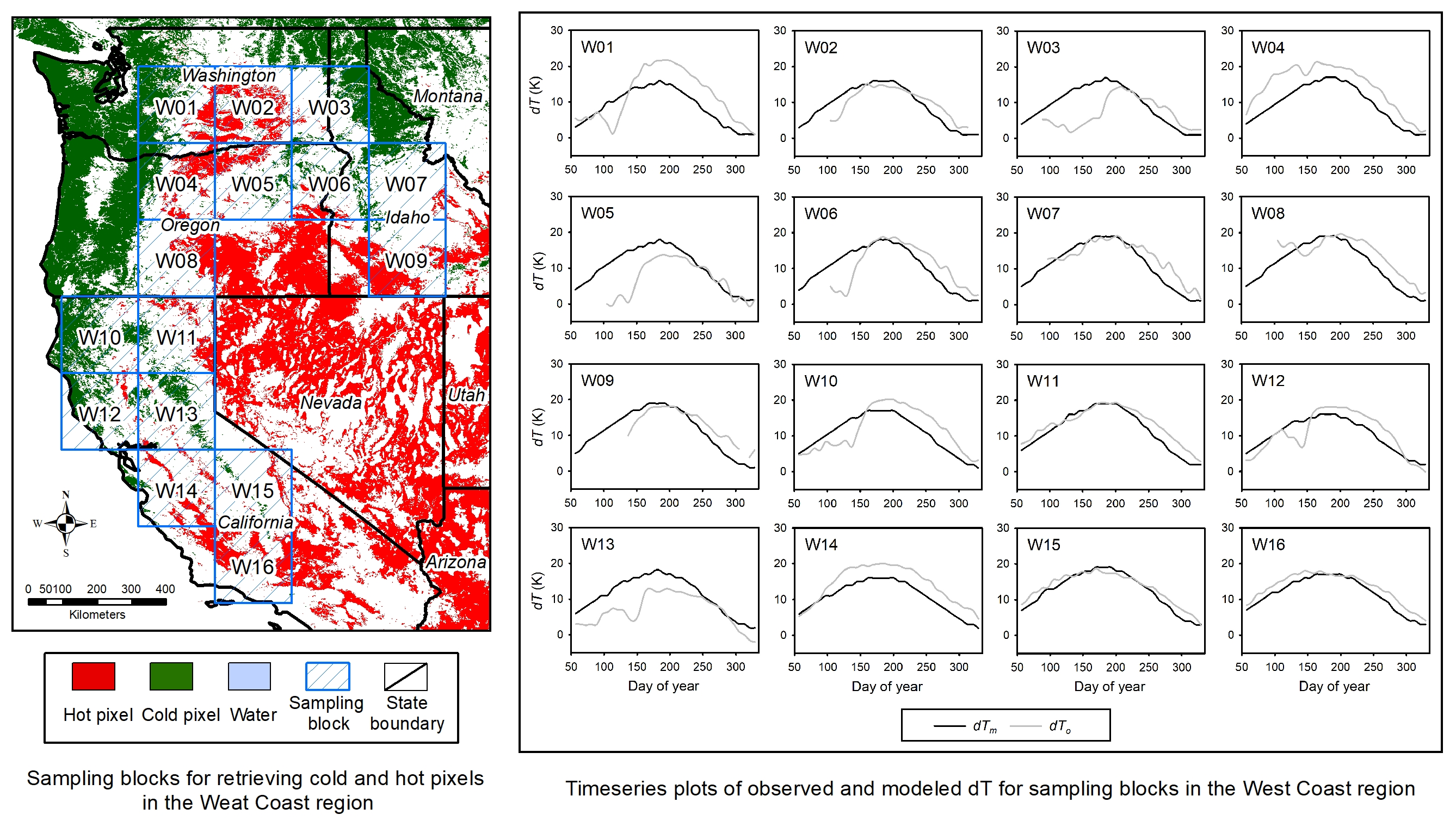
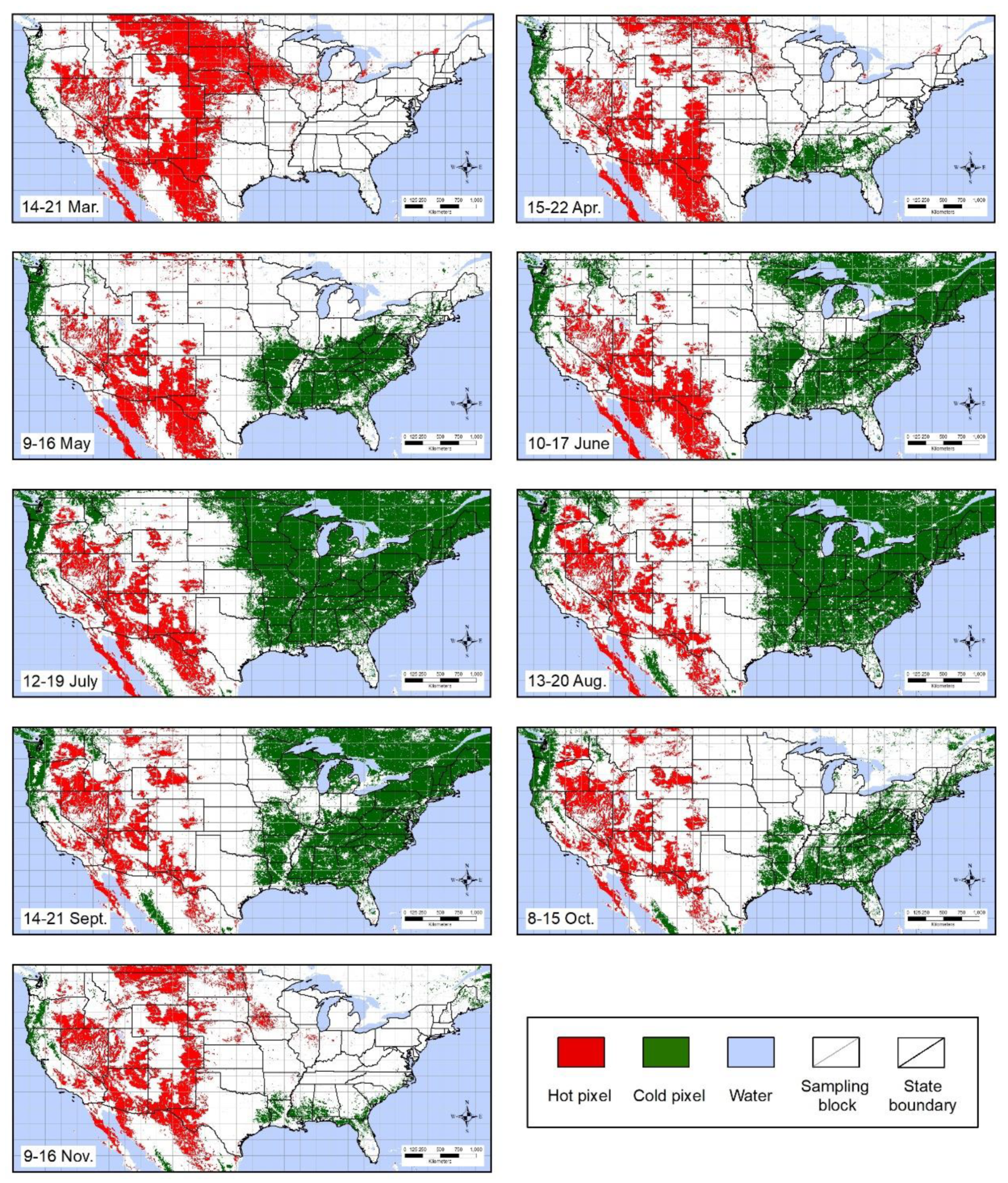
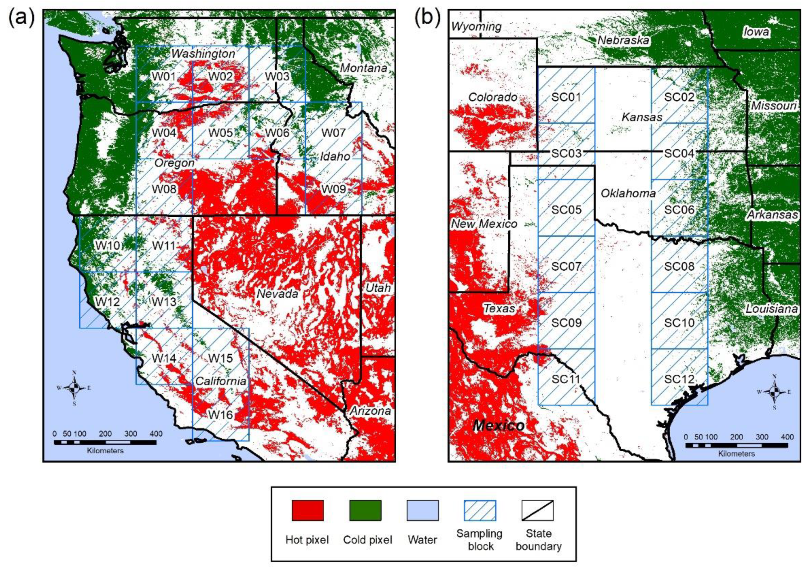
4.1. Maps of Hot and Cold Pixels

Using the 10-year average NDVI data and the stable vegetation cover map, we created maps of hot and cold pixels at 8-day interval through the year. Figure 2 demonstrates some examples of the maps of the hot and cold pixels for different months from March to November. In the maps, we notice that the hot pixels are primarily distributed in the western CONUS and the cold pixels are mostly in the eastern CONUS. The area of hot pixels is relatively consistent over different seasons, although the area is bigger in the growing season (May to October) than the non-growing season. The area of cold pixels changes dramatically throughout the year. Because of the low productivity and snow cover, there are much fewer cold pixels in the non-growing season (November to April). However, cold pixels are abundant in the central, northeastern, southeastern, and the Pacific-western CONUS in the growing season. At all locations where both hot and cold pixels existed, we extracted LSTc values from the maps through the yearly timeseries, which was used to generate the maps of T_h and T_c.

4.2. Creation of dT_o and dT_m Timeseries

For each sampling block, we used the T_h and T_c values to calculate the dT_o values (Equation 4), which were then compared with the dT_m values extracted from the same block. However, there were only a small number of blocks that contained 30 or more hot pixels and cold pixels, located mainly in the West Coast area, encompassing the states of Washington, Oregon, Idaho, and California (Figure 3a). Thus, we created the dT_o timeseries at 8-day interval throughout the year only for the blocks on the West Coast (Figure 4).

Although there were rarely good sampling blocks in other areas except for the West Coast, we were able to combine two blocks that are close to each other. We used one block containing ≥30 hot pixels and another nearby block containing ≥30 cold pixels to calculate dT_o values. In the South-Central CONUS, mainly in Kansas, Oklahoma, and Texas, we found several pairs of blocks containing more than 30 hot or cold pixels that can be combined to derive dT_o (Figure 3b). To reduce the impact of the air temperature difference between two different blocks, we combined the blocks of hot and cold pixels from the same longitude. That is, when we selected a block of hot pixels in the west side of the region, we chose a nearby block of cold pixels directly to the east. This way, we calculated dT_o values based two blocks and generated dT_o timeseries at 8-day interval throughout the year (Figure 5).

The complete dT_o timeseries consists of 46 observations (or 8-day intervals) for each sampling block. However, due to possible snow impacts on the MODIS data, we exclude the observations from the winter season (December to February). Therefore, the timeseries covers 35 observations from the 8th to 42nd 8-day interval (26 February to 2 December).

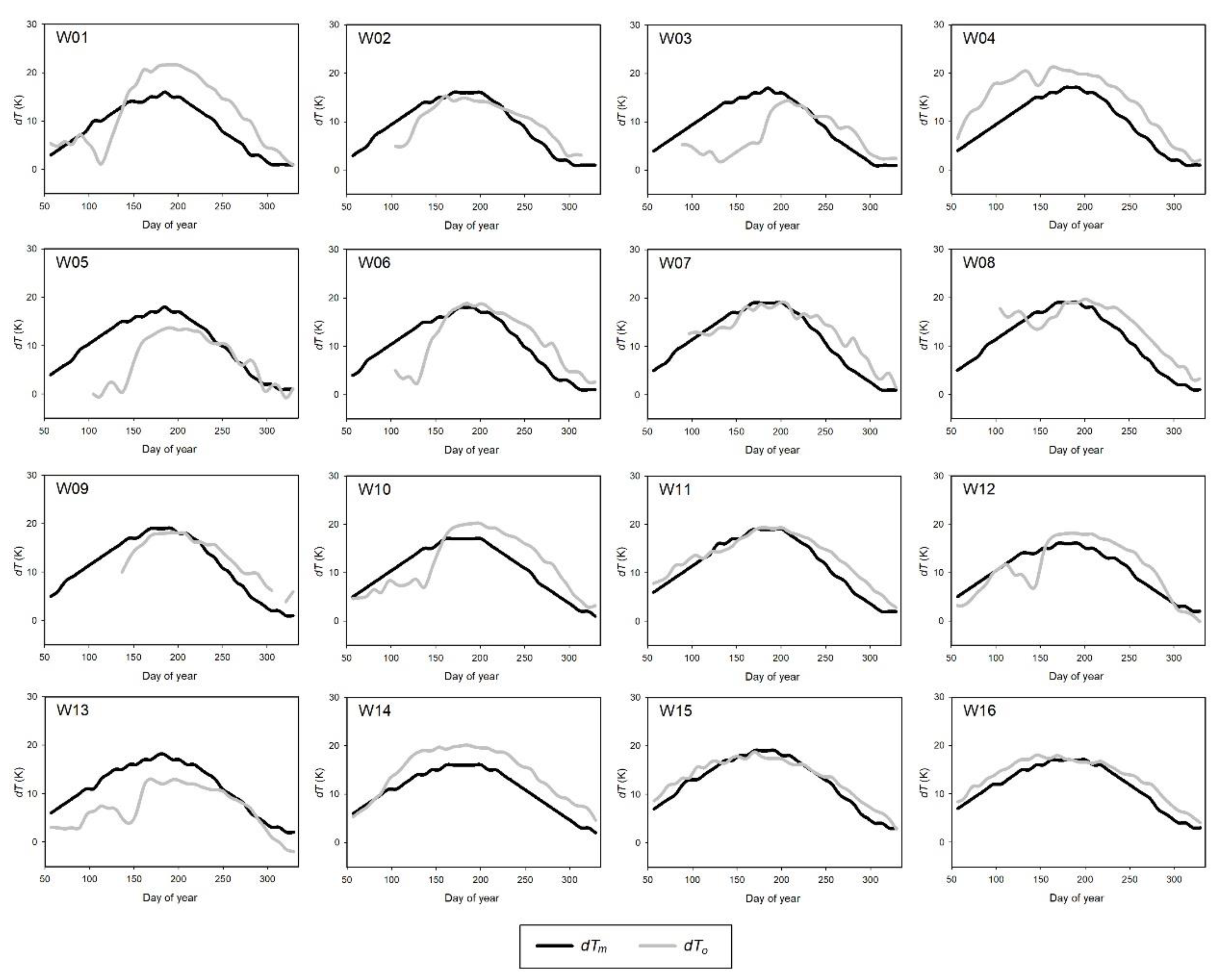
4.3. Agreement between dT_o and dT_m in the West Coast Region

Figure 3a shows the locations of the sampling blocks in the West Coast region. There are 16 blocks that meet the two requirements as the samples for generating dT_o timeseries: (1) each block contains at least 30 hot pixels and at least 30 cold pixels, and (2) the annual timeseries contains at least 2/3 of the total 35 observations (i.e., at least 24 observations) for each block. The timeseries plots of dT_o and dT_m for each block on the West Coast are shown in Figure 4. Comparing the temporal dT_o and dT_m timeseries, we found good agreement between the two variables. The overall magnitudes of dT_o and dT_m values are very close, although dT_o shows more temporal variations than dT_m. Both dT_o and dT_m also demonstrate strong seasonal patterns that show higher values in the summer with a peak between day of year 170–200 (late June to middle July) and lower values in spring and autumn. Most blocks present high agreement between dT_o and dT_m, particularly some blocks such as W07, W11, W15, and W16 showing very high agreement. Some blocks, however, show noticeable difference between dT_o and dT_m, for example, W01, W03–W06, and W13. The discrepancy between dT_o and dT_m for those blocks is probably caused by the difference in the land cover types and elevations between hot and cold pixels. Uncertainties in the MODIS NDVI and LST data may be another reason for the unstable dT_o values, which are discussed in more detail in Section 5.1.

Table 2. Agreement between modeled and observed dT values for the sample blocks in the West Coast region.

Block	Mean of dTo (K)	Mean of dTm (K)	Bias (K)	RMSE (K)	r	n
W01	11.54	8.71	2.82	5.14	0.797	35
W02	9.99	10.14	−0.16	2.74	0.862	28
W03	6.98	9.75	−2.77	5.93	0.389	32
W04	9.74	14.35	4.61	4.97	0.953	35
W05	10.79	6.96	−3.83	6.16	0.614	29
W06	11.13	11.03	0.10	4.70	0.680	29
W07	12.97	11.71	1.26	2.73	0.935	31
W08	11.93	14.05	2.12	3.38	0.910	29
W08	13.17	12.17	1.01	3.18	0.918	24
W10	11.68	10.63	1.06	3.96	0.772	35
W11	13.39	11.91	1.48	2.23	0.966	35
W12	10.65	10.26	0.39	3.01	0.855	35
W13	6.92	11.20	−4.28	5.18	0.814	35
W14	14.18	10.80	3.38	3.75	0.953	35
W15	13.31	12.51	0.79	1.57	0.978	35
W16	13.33	11.66	1.67	1.94	0.980	35
Median for all blocks	11.61	11.12	1.03	3.56	0.886	16

presents the statistics of the comparison between dT_o and dT_m for the sampling blocks in the West Coast region. The overall difference between dT_o and dT_m is low as measured with the bias (1.0 K), RMSE (3.6 K), and r value (0.89). Of all sampling blocks in this region, W15 in California shows the best agreement between dT_o and dT_m, which has a bias of 0.8 K, RMSE of 1.6 K, and r of 0.98.

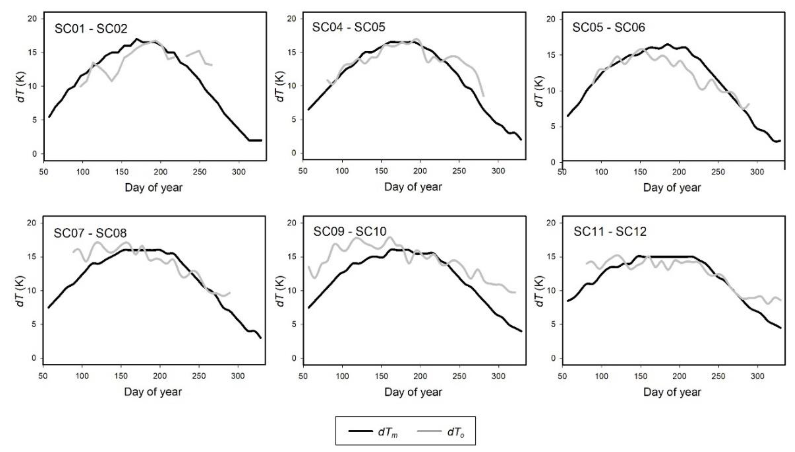
4.4. Agreement between dT_o and dT_m in the South-Central Region

For the South-Central region, because there were not enough hot and cold pixels within one single block, we combined one block containing all hot pixels and another containing all cold pixels to calculate dT_o. Figure 3b shows six pairs of hot-pixel and cold-pixel blocks in this region to generate dT_o timeseries. All hot-pixel blocks are from the western part of the region, and all cold-pixel blocks are from the eastern part.

Figure 5 shows the dT_o and dT_m timeseries plots, which demonstrate reasonably high agreement between dT_o and dT_m for all six pairs of blocks. The overall magnitudes of dT_o and dT_m values are very close, but the temporal variations of dT_o are higher than dT_m. Like dT_m, dT_o shows seasonal patterns with peaks in the growing season and lower values in spring and autumn. Compared with the West Coast region, the temporal dT_o changes in the South-central region show more apparent local variations. This is probably caused by the relatively long distance between two blocks used for calculating dT_o in this region.

Table 3. Agreement between modeled and observed dT values for the sampling blocks in the South-central region.

Block	Mean of dTo (K)	Mean of dTm (K)	Bias (K)	RMSE (K)	r	n
SC01–SC02	13.91	14.23	−0.31	2.11	0.469	20
SC03–SC04	13.84	13.35	0.49	1.55	0.879	26
SC05–SC06	12.47	13.29	−0.82	1.62	0.885	26
SC07–SC08	14.02	13.38	0.64	1.83	0.800	26
SC09–SC10	14.24	11.93	2.31	2.99	0.878	34
SC11–SC12	12.47	11.92	0.54	1.70	0.906	32
Median for all pairs of blocks	13.88	13.32	0.52	1.76	0.879	6

provides the statistics of the agreement between dT_o and dT_m timeseries for the sampling blocks, including the bias, RSME, and r between two variables for the six pairs of blocks. The overall difference between dT_o and dT_m is low, indicated by the bias (0.5K), RMSE (1.8K), and r value (0.88).

We noticed the high RMSEs for some sampling blocks from both regions, which indicate high random errors of the dT_m for those sites, but the random error could also stem from the dT_o calculated from MODIS LST, especially when the satellite observations are contaminated by clouds, cloud shadows, and snow etc. Our analysis was not able to distinguish between dT_m random error and dT_o random error. Although we assume that the dT_o based on land surface measurements has the least error compared to the model outputs, satellite-based observations are subject to measurement error to a certain degree. As we compared the timeseries plots of dT_o and dT_m (Figure 4 and Figure 5), dT_o showed more temporal variabilities than dT_m, which implied higher instability and inconsistency of the dT_o data. In this case, we tend to consider that the dT_o contributes more random error to the RMSE values than the dT_m for some blocks.

5. Discussion

5.1. Uncertainties of dT_o Estimates

In this study, we used dT_o as a reference dataset to evaluate and validate dT_m. However, because dT_o is derived from satellite data, there are several factors that may introduce uncertainties to the dT_o observations. First, the MODIS LST data are subject to measurement and estimation errors that can be transferred to the dT_o calculation. Second, MODIS NDVI data contain errors caused by background soil, atmospheric effect, nonlinear relationship to vegetation fraction, and saturation for dense vegetation cover, etc. Because NDVI values of 0.25 and 0.7 are the thresholds for identifying hot and cold pixels in this study, errors in NDVI will result in confusion in the counts of hot and cold pixels within the sampling block. Third, contaminations from clouds, cloud shadows, snow cover, and fires may influence the quality of the LST and NDVI images. Although we created a suite of data masks based on the MODIS reflectance QA and fire data to eliminate the poor-quality pixels, residuals of clouds, cloud shadows, snow cover, and fires may still exist. Fourth, the difference in temperature between different elevations may cause errors in the dT_o estimation. For each sampling block, the hot and cold pixels may be located at different elevations, which will induce bias in dT_o estimates if the elevation difference is substantial. Although this issue is partially resolved by using the lapse rate (Equation 3) to correct the LST in the study, the lapse rate we used is a general rate. For a specific site, the lapse rate is affected by the variations in the local temperature profile. Lastly, as the dT_o values are calculated from hot and cold pixels located at different sites within a sampling block, errors in dT_o may be induced if the hot and cold pixels are located at different LST gradients. The impact of the LST gradient is more noticeable in the South-Central region where the dT_o calculation uses the hot and cold pixels from two separate blocks.

Among all those factors, uncertainty in LST is the most influential one in the accuracy of the dT_o calculation. Validation and evaluation of MODIS LST data have been well conducted and documented previously [38,39,40,41]. For example, Coll et al. 2009 validated the MODIS LST (Collection 5) product over rice fields in Spain and forest sites in Germany using the temperature-based and the radiance-based methods [42]. Their analysis showed an average bias of −0.3 to −0.4 K and RMSE of 0.6–0.7 K between MODIS LST and in situ LST using the two validation methods. Guillevic et al. 2012 validated the MODIS LST (Collection 5) product at an agricultural testing site in Illinois, USA, using a land surface modeling approach that scaled up ground LST measurements from field and weather stations to satellite data resolution [39]. They found an absolute error of 0.0 K and RMSE of 2.0 K for the MODIS LST product. Li et al. 2014 evaluated MODIS LST product (MOD11_L2 and MYD_L2, Collection 5) in an arid area of Northwest China and reported that the product underestimated the LST for the barren surface sites, with biases varying from −3.13 K to 0.31 K and RMSEs varying from 1.04 to 3.16 K [43]. Krishnan et al. 2015 compared the MODIS LST (MOD11A and MYD11A, Collection 5) data with LST measurements from infrared temperature sensors at micrometeorological tower sites and from aircraft campaigns over a mixed grassland forest site in Tennessee, USA [44]. Their study showed that the MODIS LST (including both daytime and nighttime data) had a bias of −0.56 K and RMSE of 2.84 K compared to the tower-based LST records at the site. Since 2016, the newest collection (Collection 6) MODIS LST data have been produced and are available for the user community. Collection 6 has implemented refinements, resulting in better data quality than Collection 5. Duan et al. 2018 validated the MODIS LST Collection 6 product using 38 validation sites over eight worldwide land cover types [38]. They found good agreement between MODIS LST and radiance-based LST values, with bias and RMSE values less than 1 K for most sites during the daytime and nighttime. As a summary of the previous studies, the bias of the MODIS LST data is generally lower than 1 K, but the random error can be up to 3 K. In our data analysis, as we calculated 10-year average LST, the temporal random errors in LST can be reduced to a certain degree.

5.2. Error Sources and Ranges of dT_m Estimation

In the SSEBop model, the predefined dT_m parameter is derived from the surface energy balance equation under the average sky condition where latent heat flux and ground heat flux on a daily time scale are assumed to be zero, and sensible heat is assumed to be maximum [14]. According to the SSEBop formulation, the uncertainties of dT_m depend not only on multiple assumptions, but also on the errors of input parameters and variables, including net radiation (Rn) on the surface, aerodynamic resistance to heat transfer (r_ah), air density (ρ_a), and specific heat air (C_p). Rn is the difference between net shortwave radiation (Rns) and net longwave radiation (Rnl), which is the function of albedo (α), incoming solar radiation (R_s), extraterrestrial solar radiation (R_a), minimum and maximum air temperature (T_min and T_max), and elevation (z). Chen et al. 2016 summarized the error sources and ranges of the input parameters and variables in the SSEBop algorithm [21]. For example, the error ranges are 0.5–3% for α, 1.2–10% for R_a, 5–15% for T_min and T_max, and 0.6–3.6% for r_ah (0.6–3.6%) [21]. Based on the statistical analysis of the uncertainty and sensitivity of the SSEBop model using the eddy covariance measurements at 42 AmeriFlux tower sites across the CONUS, dT_m is sensitive to errors of R_a, α, r_ah, C_p, T_max, T_min, and z, listed in order from the most to the least sensitive [21]. Their study indicates that the reduction of errors from input variables (i.e., ETa and LST) and key parameters (i.e., dT_m and T_max) can significantly improve the SSEBop ETa calculation. Their study also suggests that error of the dT_m be constrained to be less than ±2 to ±5 K for the growing season and less than ±1 to ±2.5 K for the non-growing season in order to limit the relative error of ETa estimation lower than 20% [21]. Our current study on the evaluation of the dT_m estimates with satellite-based dT_o indicates that the error of the dT_m is generally lower than the basic requirements for the SSEBop model.

6. Conclusions

The high-quality ET product generated by the SSEBop model relies decisively on the accuracy of the dT_m estimates. In this study, we evaluated the dT_m data using satellite observations including NDVI and LST to identify hot and cold pixels and retrieved dT_o from those pixels. We generated the seasonal dT_o and dT_m timeseries for each sampling block across the CONUS and made comparisons between the two variables. Only in the West Coast region was there a good number of sampling blocks containing enough hot and cold pixels for generating dT_o timeseries. Meanwhile, in the South-Central region, we used nearby sampling blocks that contain only hot or cold pixels to create the dT_o timeseries. As a result, the evaluation of the dT_m product was conducted by comparing it with the dT_o values for all available sampling blocks in the West Coast and South-Central regions. The results showed high agreement between the seasonal dT_o and dT_m timeseries in both regions. The quantitative comparison between dT_o and dT_m indicated bias = 1.0 K, RMSE = 3.6 K, and r = 0.89 for the West Coast region, and bias = 0.5 K, RMSE = 1.8 K, and r = 0.88 for the South-Central region. Through this analysis, we conclude that the dT_m estimation from the SSEBop model is reliable, which further assures the desirable accuracy of the ETa estimation.

As one of the two key parameters in the SSEBop model, dT defines the hot/dry limit of the model using theoretical calculations. The theoretical determination of dT enables the SSEBop model to be operationalized and applied to regional and global scales by eliminating the need for manually collecting the dry limit from images. However, the capability for the automation does not compromise the accuracy of the parameter, which could have a marked influence on the magnitude of ETa estimation. Using a commonly observed value of dT = 20 K for the peak growing season in the Southwestern United States, an error of 2 K from dT estimation could translate into a 10% error in ET estimation [13,21]. Thus, reasonable agreement between theoretical and observed dT values, as discovered in this study, will not only save time in ET modeling but also improve the consistency and reliability of the ET estimation at multi-spatiotemporal scales.

References

1. Amatya, D.M.; Irmak, S.; Gowda, P.; Sun, G.; Nettles, J.E.; Douglas-Mankin, K.R. Ecosystem evapotranspiration: Challenges in measurements, estimates, and modeling. Trans. ASABE 2016, 59, 555–560. [Google Scholar]
2. Gowda, P.H.; Chavez, J.L.; Colaizzi, P.D.; Evett, S.R.; Howell, T.A.; Tolk, J.A. ET mapping for agricultural water management: Present status and challenges. Irrig. Sci. 2008, 26, 223–237. [Google Scholar] [CrossRef]
3. Li, Z.-L.; Tang, R.; Wan, Z.; Bi, Y.; Zhou, C.; Tang, B.; Yan, G.; Zhang, X. A review of Current methodologies for regional evapotranspiration estimation from remotely sensed Data. Sensors 2009, 9, 3801–3853. [Google Scholar] [CrossRef] [PubMed]
4. Xu, C.-Y.; Singh, V.P. Evaluation of three complementary relationship evapotranspiration models by water balance approach to estimate actual regional evapotranspiration in different climatic regions. J. Hydrol. 2005, 308, 105–121. [Google Scholar] [CrossRef]
5. Menenti, M.; Choudhury, B.J. Parameterization of land surface evapotranspiration using a location-dependent potential evapotranspiration and surface temperature range. In Exchange Processes at the Land Surface for a Range of Space and Time Scales, Proceedings of the Yokohama Symposium, Yokohama, Japan, 26–30 July 1993; Bolle, H.J., Feddes, R.A., Kalma, J.D., Eds.; International Association of Hydrological Sciences Publication No. 212; IAHS Press: Wallingford, Oxfordshire, UK, 1993; pp. 561–568. [Google Scholar]
6. Norman, J.M.; Divakarla, M.; Goel, N.S. Algorithms for extracting information from remote thermal-IR observations of the Earth’s surface. Remote Sens. Environ. 1995, 51, 157–168. [Google Scholar] [CrossRef]
7. Bastiaanssen, W.G.M.; Menenti, M.; Feddes, R.A.; Holtslag, A.A.M. A remote sensing surface energy balance algorithm for land (SEBAL) 1. Formulation. J. Hydrol. 1998, 212, 198–212. [Google Scholar] [CrossRef]
8. Bastiaanssen, W.G.M.; Pelgrum, H.; Wang, J.; Ma, Y.; Moreno, J.F.; Roerink, G.J.; van der Wal, T. A remote sensing surface energy balance algorithm for land (SEBAL) 2. Validation. J. Hydrol. 1998, 212, 213–229. [Google Scholar] [CrossRef]
9. Roerink, G.J.; Su, Z.; Menenti, M. S-SEBI: A simple remote sensing algorithm to estimate the surface energy balance. Phys. Chem. Earth Part B Hydrol. Oceans Atmos. 2000, 25, 147–157. [Google Scholar] [CrossRef]
10. Su, Z. The Surface Energy Balance System (SEBS) for estimation of turbulent heat fluxes. Hydrol. Earth Syst. Sci. 2002, 6, 85–99. [Google Scholar] [CrossRef]
11. Allen, R.G.; Tasumi, M.; Trezza, R. Satellite-based energy balance for mapping evapotranspiration at high resolution with internalized calibration (METRIC)—Model. J. Irrig. Drain. Eng. 2007, 133, 380–394. [Google Scholar] [CrossRef]
12. Allen, R.G.; Tasumi, M.; Morse, A.; Trezza, R.; Wright, J.L.; Bastiaanssen, W.; Kramber, W.; Lorite, I.; Robison, C.W. Satellite-based energy balance for mapping evapotranspiration with internalized calibration (METRIC)—Applications. J. Irrig. Drain. Eng. 2007, 133, 395–406. [Google Scholar] [CrossRef]
13. Senay, G.B.; Bohms, S.; Singh, R.K.; Gowda, P.H.; Velpuri, N.M.; Alemu, H.; Verdin, J.P. Operational evapotranspiration mapping using remote sensing and weather datasets: A new parameterization for the SSEB approach. J. Am. Water Resour. Assoc. 2013, 49, 577–591. [Google Scholar] [CrossRef]
14. Senay, G.B. Satellite psychrometric formulation of the Operational Simplified Surface Energy Balance (SSEBop) model for quantifying and mapping evapotranspiration. Appl. Eng. Agric. 2018, 34, 555–566. [Google Scholar] [CrossRef]
15. Senay, G.B.; Budde, M.; Verdin, J.P.; Melesse, A.M. A coupled remote sensing and simplified surface energy balance approach to estimate actual evapotranspiration from irrigated fields. Sensors 2007, 7, 979–1000. [Google Scholar] [CrossRef]
16. Senay, G.B.; Budde, M.E.; Verdin, J.P. Enhancing the Simplified Surface Energy Balance (SSEB) approach for estimating landscape ET: Validation with the METRIC model. Agric. Water Manag. 2011, 98, 606–618. [Google Scholar] [CrossRef]
17. Senay, G.B.; Leake, S.; Nagler, P.L.; Artan, G.; Dickinson, J.; Cordova, J.T.; Glenn, E.P. Estimating basin scale evapotranspiration (ET) by water balance and remote sensing methods. Hydrol. Process. 2011, 25, 4037–4049. [Google Scholar] [CrossRef]
18. Senay, G.B.; Schauer, M.; Velpuri, N.M.; Singh, R.K.; Kagone, S.; Friedrichs, M.; Litvak, M.E.; Douglas-Mankin, K.R. Long-term (1986–2015) crop water use characterization over the Upper Rio Grande Basin of United States and Mexico using Landsat-based evapotranspiration. Remote Sens. 2019, 11, 1587. [Google Scholar] [CrossRef]
19. Senay, G.B.; Schauer, M.; Friedrichs, M.; Velpuri, N.M.; Singh, R.K. Satellite-based water use dynamics using historical Landsat data (1984–2014) in the southwestern United States. Remote Sens. Environ. 2017, 202, 98–112. [Google Scholar] [CrossRef]
20. Senay, G.B.; Friedrichs, M.; Singh, R.K.; Velpuri, N.M. Evaluating Landsat 8 evapotranspiration for water use mapping in the Colorado River Basin. Remote Sens. Environ. 2016, 185, 171–185. [Google Scholar] [CrossRef] [Green Version]
21. Chen, M.; Senay, G.B.; Singh, R.K.; Verdin, J.P. Uncertainty analysis of the Operational Simplified Surface Energy Balance (SSEBop) model at multiple flux tower sites. J. Hydrol. 2016, 536, 384–399. [Google Scholar] [CrossRef] [Green Version]
22. Velpuri, N.M.; Senay, G.B.; Singh, R.K.; Bohms, S.; Verdin, J.P. A comprehensive evaluation of two MODIS evapotranspiration products over the conterminous United States: Using point and gridded FLUXNET and water balance ET. Remote Sens. Environ. 2013, 139, 35–49. [Google Scholar] [CrossRef]
23. Weerasinghe, I.; van Griensven, A.; Bastiaanssen, W.; Mul, M.; Jia, L. Can we trust remote sensing ET products over Africa? Hydrol. Earth Syst. Sci. 2019. under review. [Google Scholar] [CrossRef]
24. Mu, Q.; Heinsch, F.A.; Zhao, M.; Running, S.W. Development of a global evapotranspiration algorithm based on MODIS and global meteorology data. Remote Sens. Environ. 2007, 111, 519–536. [Google Scholar] [CrossRef]
25. Mu, Q.; Zhao, M.; Running, S.W. Improvements to a MODIS Global Terrestrial Evapotranspiration Algorithm. Remote Sens. Environ. 2011, 115, 1781–1800. [Google Scholar] [CrossRef]
26. Jung, M.; Reichstein, M.; Bondeau, A. Towards global empirical upscaling of FLUXNET eddy covariance observations: Validation of a model tree ensemble approach using a biosphere model. Biogeosciences 2009, 6, 2001–2013. [Google Scholar]
27. Alemayehu, T.; van Griensven, A.; Senay, G.B.; Bauwens, W. Evapotranspiration mapping in a heterogeneous landscape using remote sensing and global weather datasets: Application to the Mara Basin, East Africa. Remote Sens. 2017, 9, 390. [Google Scholar] [CrossRef]
28. Bhattarai, N.; Shaw, S.B.; Quackenbush, L.J.; Im, J.; Niraula, R. Evaluating five remote sensing based single-source surface energy balance models for estimating daily evapotranspiration in a humid subtropical climate. Int. J. Appl. Earth Obs. Geoinf. 2016, 49, 75–86. [Google Scholar] [CrossRef]
29. Bhattarai, N.; Mallick, K.; Stuart, J.; Vishwakarma, B.D.; Niraula, R.; Sen, S.; Jain, M. An automated multi-model evapotranspiration mapping framework using remotely sensed and reanalysis data. Remote Sens. Environ. 2019, 229, 69–92. [Google Scholar] [CrossRef]
30. Senkondo, W.; Munishi, S.E.; Tumbo, M.; Nobert, J.; Lyon, S.W. Comparing remotely-sensed surface energy balance evapotranspiration estimates in heterogeneous and data-limited regions: A case study of Tanzania’s Kilombero Valley. Remote Sens. 2019, 11, 1289. [Google Scholar] [CrossRef]
31. Singh, R.K.; Senay, G.B. Comparison of four different energy balance models for estimating evapotranspiration in the Midwestern United States. Water 2016, 8, 9. [Google Scholar] [CrossRef]
32. MCD12Q1 v006. Available online: https://lpdaac.usgs.gov/products/mcd12q1v006/ (accessed on 11 June 2019).
33. PRISM Climate Data. Available online: http://prism.oregonstate.edu (accessed on 11 June 2019).
34. AppEEARS. Available online: https://lpdaac.usgs.gov/tools/appeears/ (accessed on 11 June 2019).
35. Thornton, P.E.; Thornton, M.M.; Mayer, B.W.; Wei, Y.; Devarakonda, R.; Vose, R.S.; Cook, R.B. Daymet: Daily Surface Weather Data on a 1-km Grid for North America Version 3; ORNL DAAC: Oak Ridge, TN, USA, 2018. [Google Scholar] [CrossRef]
36. Daymet. Available online: https://daymet.ornl.gov/ (accessed on 11 June 2019).
37. Danielson, J.J.; Gesch, D.B. Global Multi-resolution Terrain Elevation Data 2010 (GMTED2010). In U.S. Geological Survey Open-File Report 2011–1073; U.S. Geological Survey: Reston, VA, USA, 2011. [Google Scholar]
38. Duan, S.B.; Li, Z.L.; Wu, H.; Leng, P.; Gao, M.; Wang, C. Radiance-based validation of land surface temperature products derived from Collection 6 MODIS thermal infrared data. Int. J. Appl. Earth Obs. Geoinf. 2018, 70, 84–92. [Google Scholar] [CrossRef]
39. Guillevic, P.C.; Privette, J.L.; Coudert, B.; Palecki, M.A.; Demarty, J.; Ottlé, C.; Augustine, J.A. Land Surface Temperature product validation using NOAA’s surface climate observation networks—Scaling methodology for the Visible Infrared Imager Radiometer Suite (VIIRS). Remote Sens. Environ. 2012, 124, 282–298. [Google Scholar] [CrossRef]
40. Li, Z.L.; Tang, B.H.; Wu, H.; Ren, H.; Yan, G.; Wan, Z.; Trigo, I.F.; Sobrino, J.A. Satellite-derived land surface temperature: Current status and perspectives. Remote Sens. Environ. 2013, 131, 14–37. [Google Scholar] [CrossRef] [Green Version]
41. Wan, Z.; Zhang, Y.; Zhang, Q.; Li, Z. Validation of the land-surface temperature products retrieved from Terra Moderate Resolution Imaging Spectroradiometer data. Remote Sens. Environ. 2002, 83, 163–180. [Google Scholar] [CrossRef]
42. Coll, C.; Wan, Z.; Galve, J.M. Temperature-based and radiance-based validations of the V5 MODIS land surface temperature product. J. Geophys. Res. 2009, 114, D20102. [Google Scholar] [CrossRef]
43. Li, H.; Sun, D.; Yu, Y.; Wang, H.; Liu, Y.; Liu, Q.; Du, Y.; Wang, H.; Cao, B. Evaluation of the VIIRS and MODIS LST products in an arid area of Northwest China. Remote Sens. Environ. 2014, 142, 111–121. [Google Scholar] [CrossRef] [Green Version]
44. Krishnan, P.; Kochendorfer, J.; Dumas, E.J.; Guillevic, P.C.; Baker, C.B.; Meyers, T.P.; Martos, B. Comparison of in-situ, aircraft, and satellite land surface temperature measurements over a NOAA Climate Reference Network site. Remote Sens. Environ. 2015, 165, 249–264. [Google Scholar] [CrossRef]
Figure 1. Map of the study area showing the 2° × 2° (approximately 200 km) sampling blocks and examples of the 10-year (2008–2017) average land surface temperature (LST) and normalized difference vegetation index (NDVI) images for 12–19 July. (a) LST. (b) NDVI. Data source: Moderate Resolution Imaging Spectroradiometer (MODIS) Collection 6 MYD11A2 and MYD09A1 (Table 1).
Remotesensing 11 01947 g001
Figure 2. Maps of hot and cold pixels created based on the 10-year average (2008–2017) LST and NDVI images. The label of each map indicates the dates of the beginning and the end of the 8-day interval.
Remotesensing 11 01947 g002
Figure 3. Sampling blocks used for retrieving LST from hot and cold pixels to calculate observed dT (dTo). The date of the hot and cold pixels in the map is 12–19 July. (a) West Coast region. (b) South-Central region.
Remotesensing 11 01947 g003
Figure 4. Timeseries plots of dTo and dT (dTm) for the sample blocks in the West Coast region. The label in each plot indicates the name of the sampling block shown in Figure 3.
Remotesensing 11 01947 g004
Figure 5. Timeseries plots of dTo and dTm for the sample blocks in the South-Central region. The labels in each plot indicates the paired sampling blocks shown in Figure 3.
Remotesensing 11 01947 g005