Estimating Stand Age from Airborne Laser Scanning Data to Improve Models of Black Spruce Wood Density in the Boreal Forest of Ontario

Abstract
:
1. Introduction
2. Materials and Methods
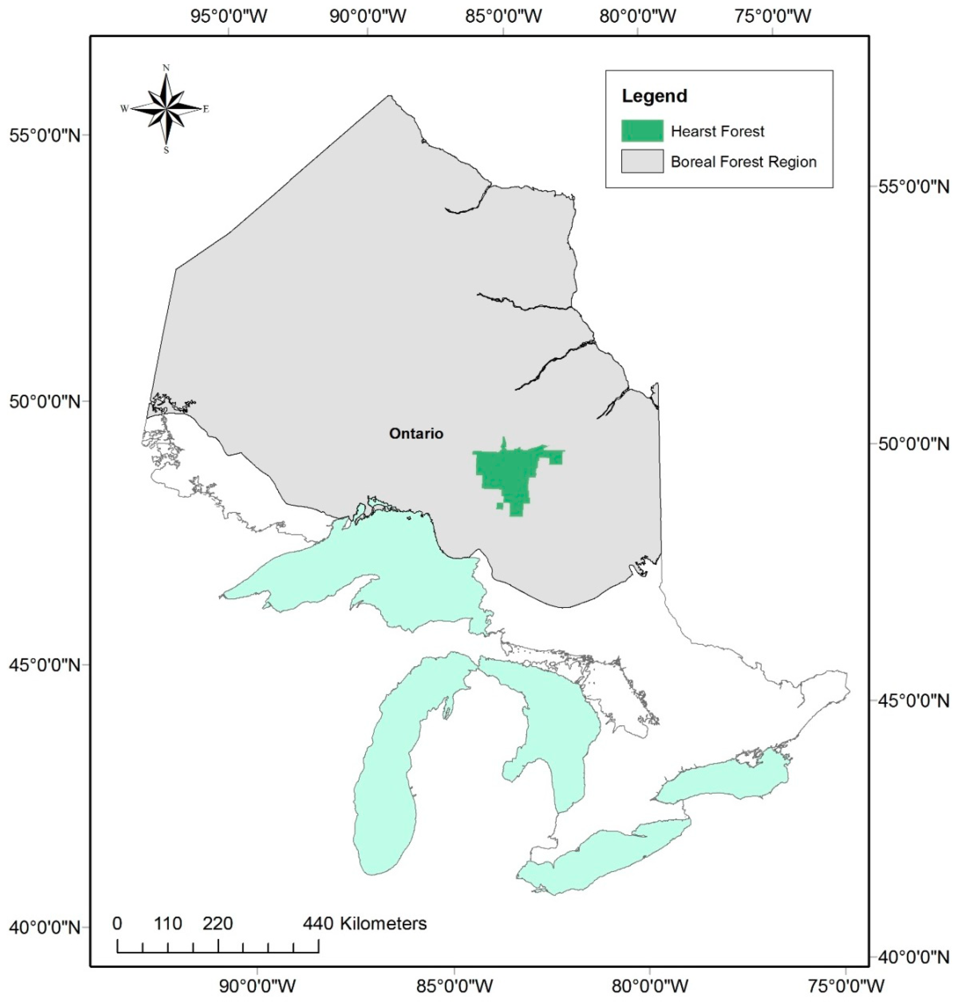
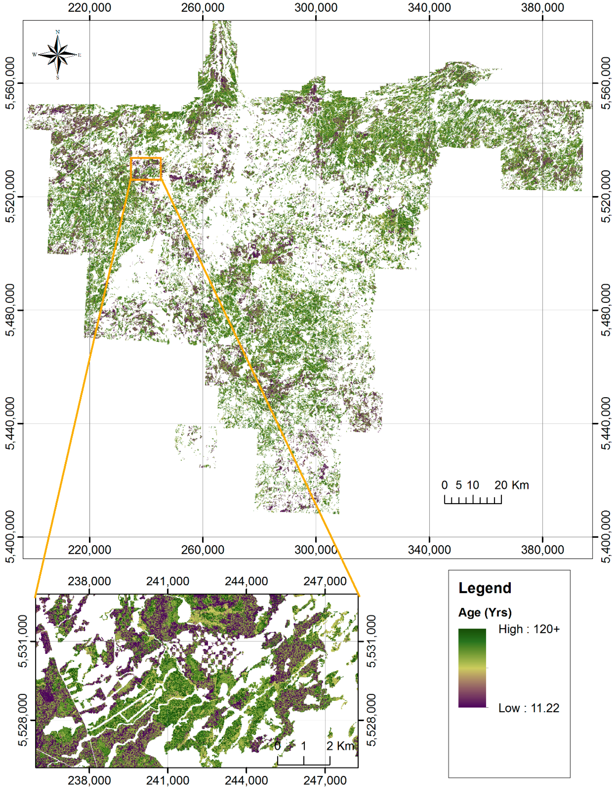
2.1. Study Area
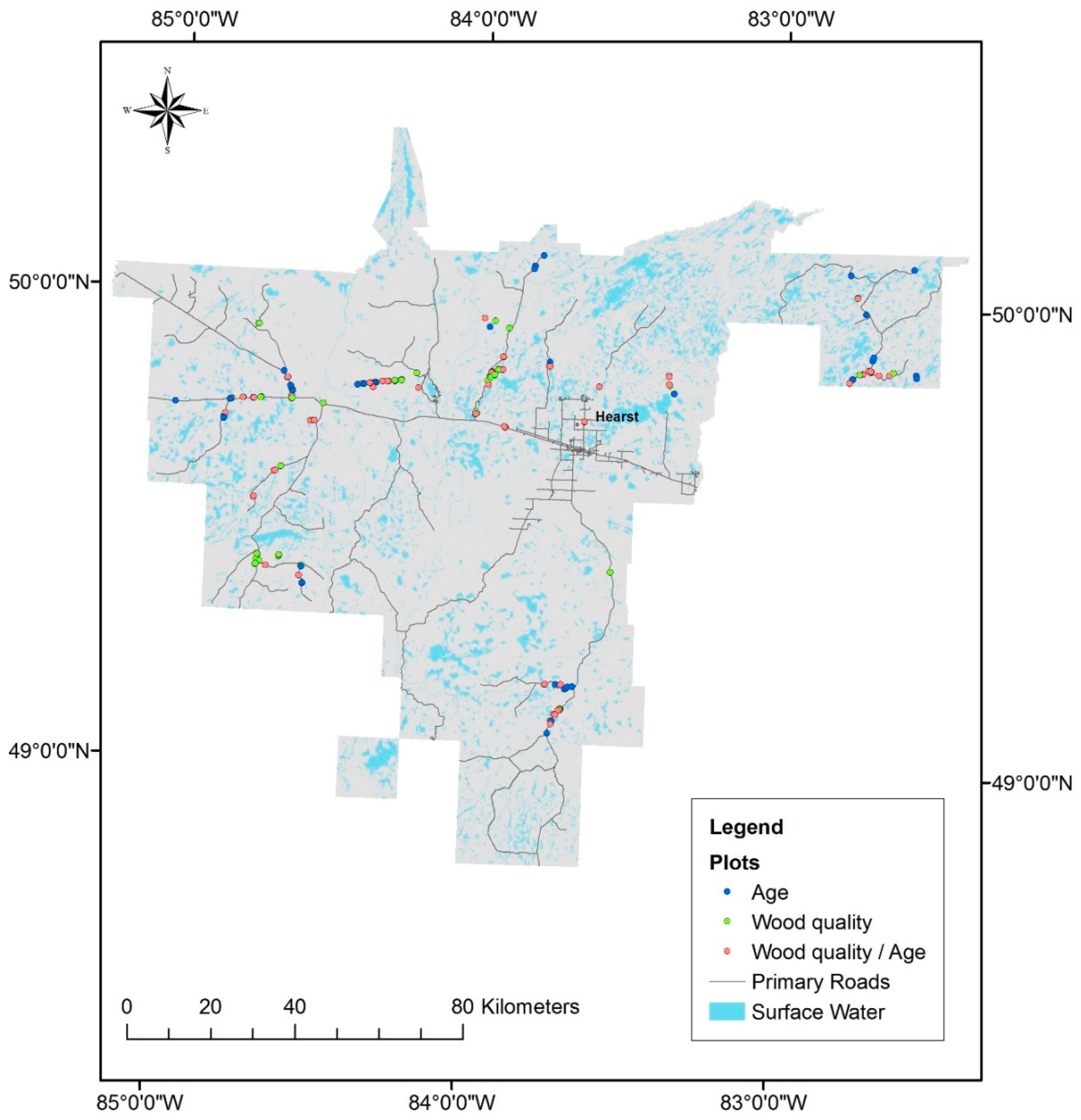
2.2. Sampling Design
2.3. Age Modeling
2.4. Wood Density Modeling
3. Results
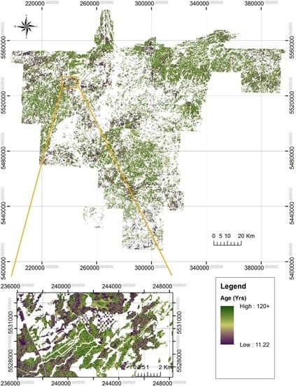
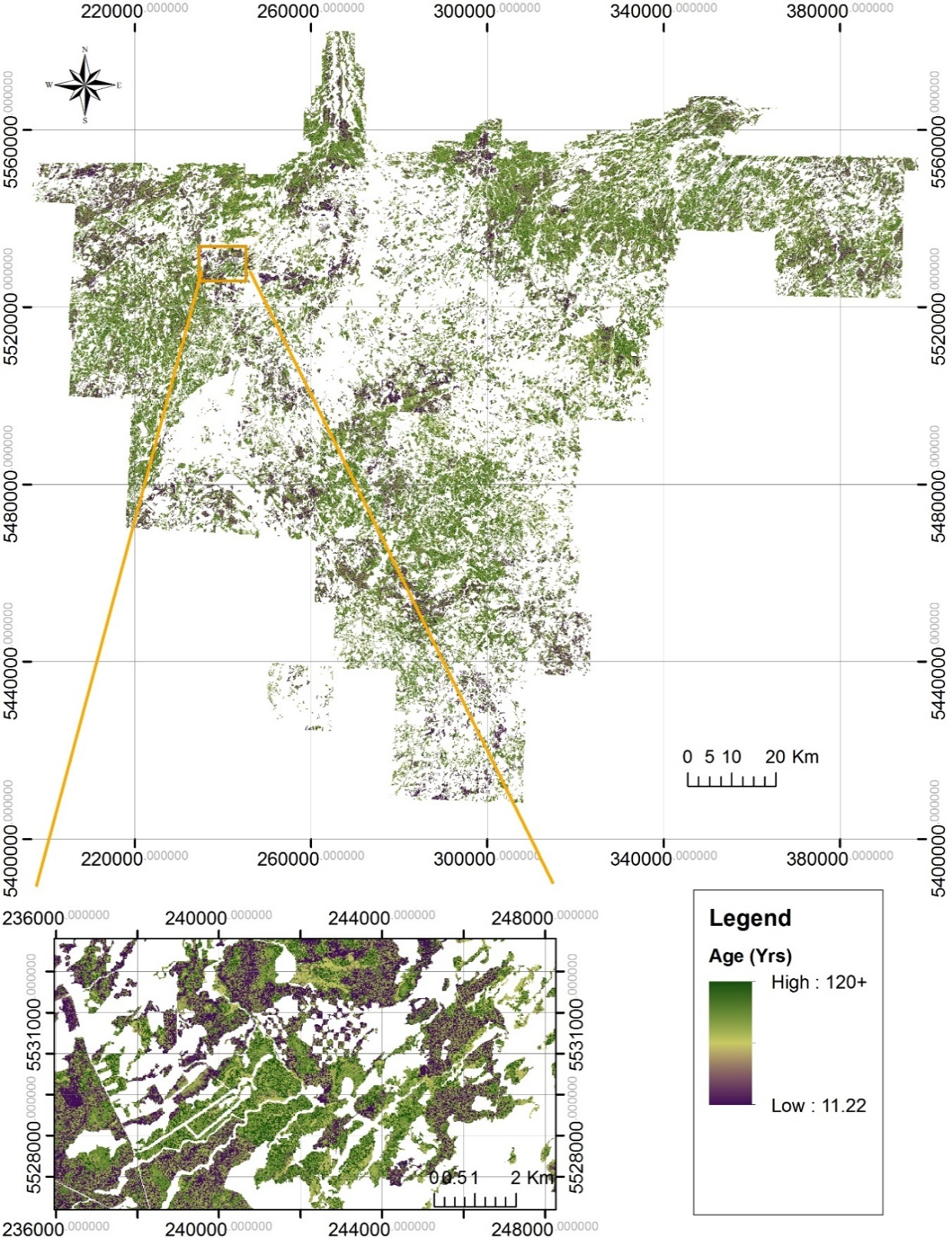
3.1. Age Modeling
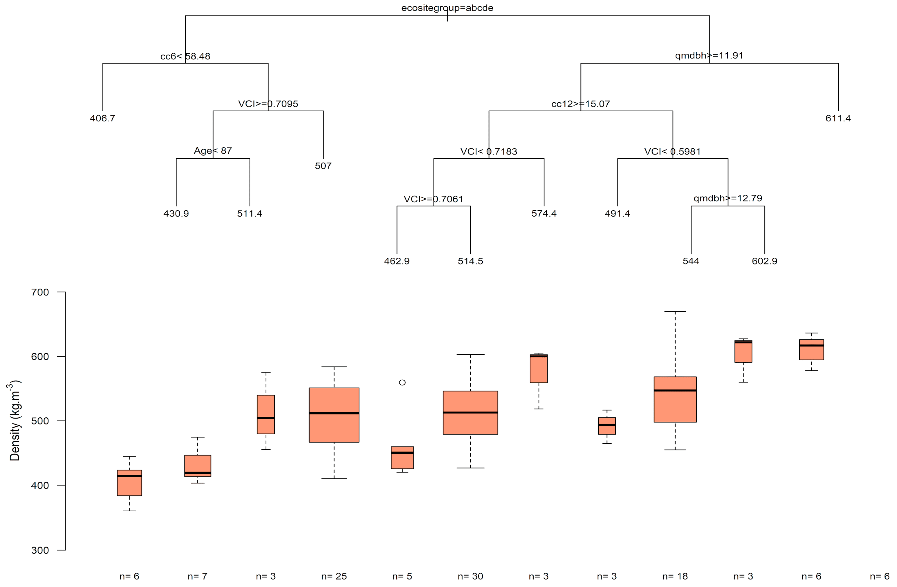
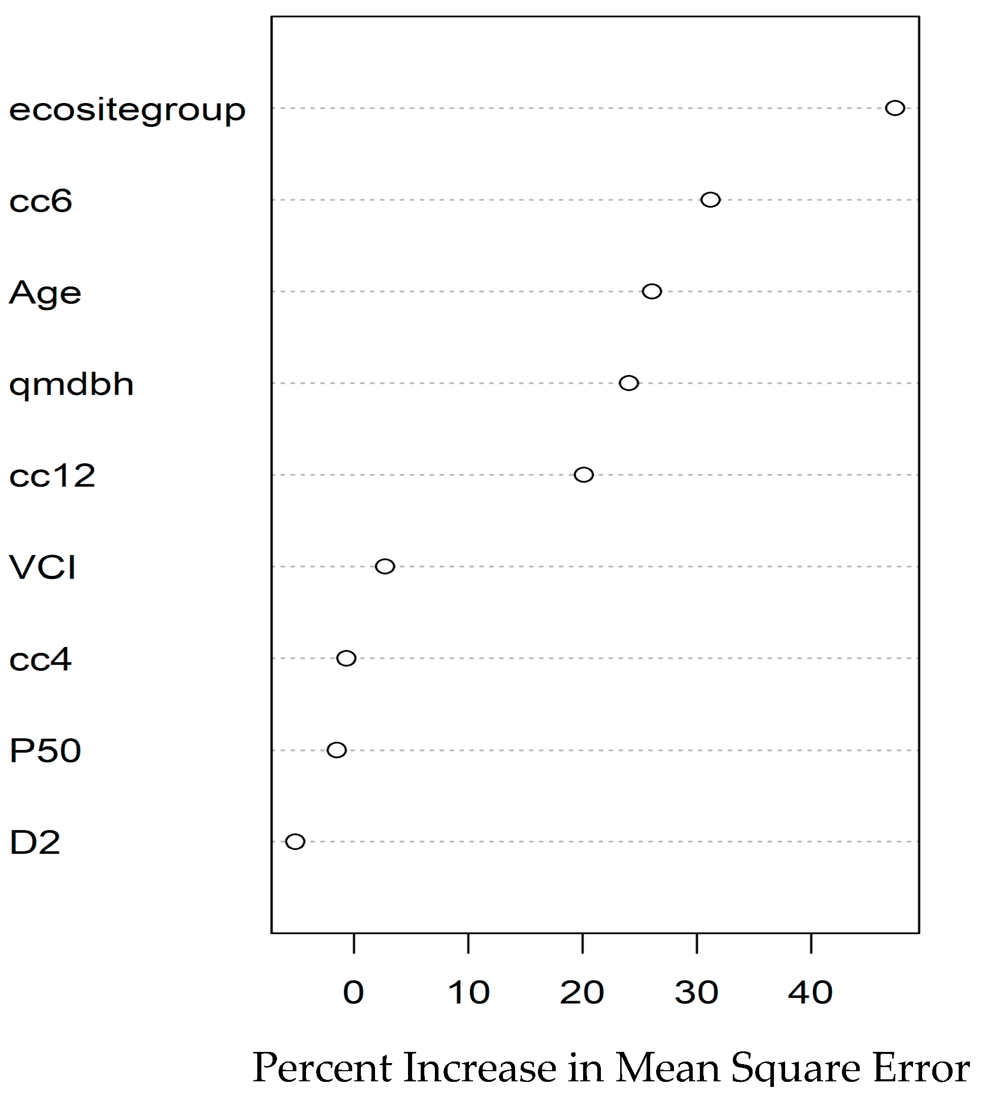
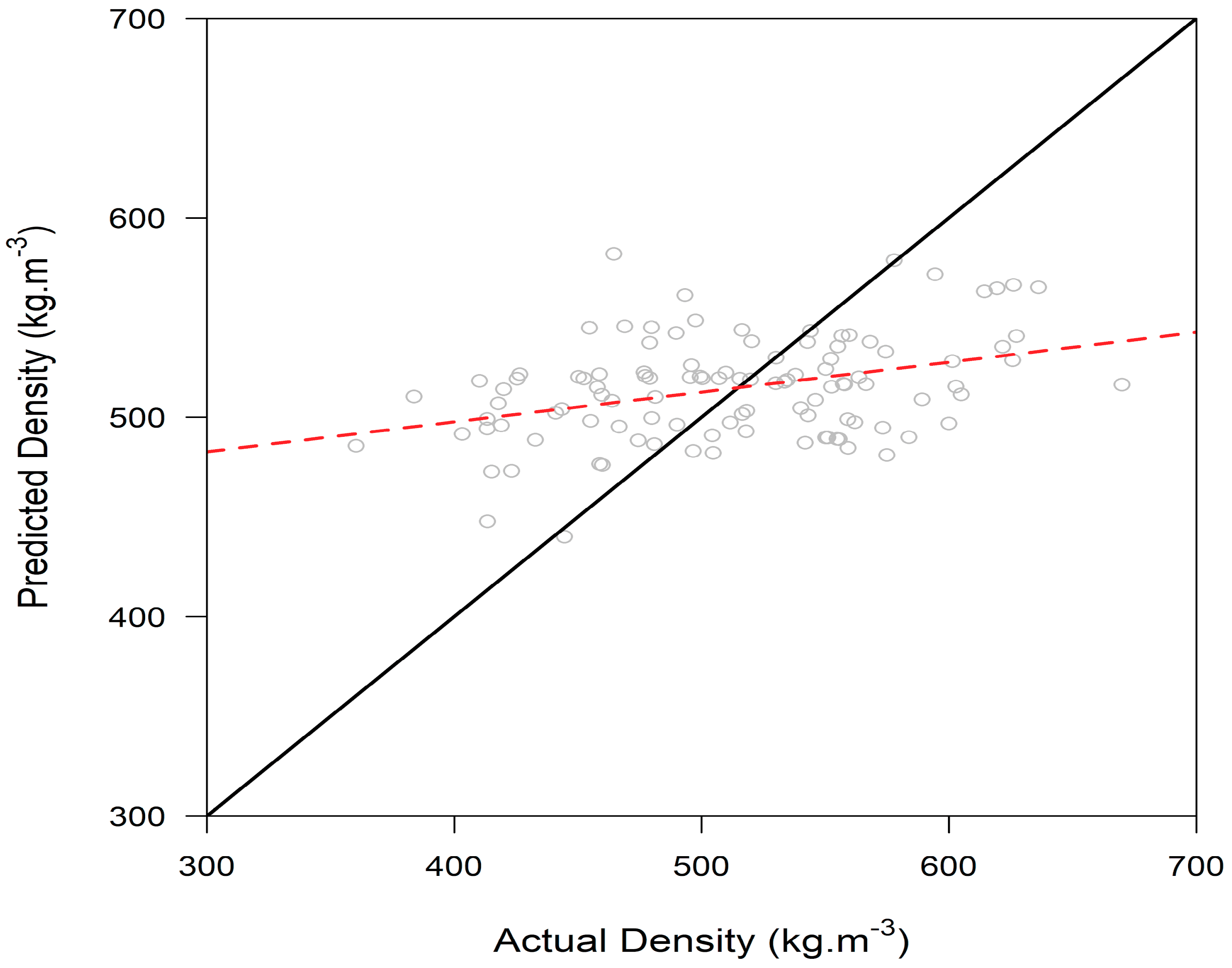
3.2. Wood Density Modeling
4. Discussion
4.1. Age Prediction
4.2. Wood Density Modeling
5. Conclusions
Author Contributions
Funding
Acknowledgments
Conflicts of Interest
References
- Treitz, P.; Lim, K.; Woods, M.; Pitt, D.; Nesbitt, D.; Etheridge, D. LiDAR sampling density for forest resource inventories in Ontario, Canada. Remote Sens. 2012, 4, 830–848. [Google Scholar] [CrossRef]
- Racine, E.B.; Coops, N.C.; St-Onge, B.; Begin, J. Forest stand age from LiDAR—Derived predictors and nearest neighbor imputation. For. Sci. 2014, 60, 128–136. [Google Scholar] [CrossRef]
- Luther, J.E.; Skinner, R.; Fournier, R.A.; van Lier, O.R.; Bowers, W.W.; Cote, J.-F.; Hopkinson, C.; Moulton, T. Predicting wood quantity and quality attributes of balsam fir and black spruce using airborne laser scanner data. Forestry 2013, 87, 1–14. [Google Scholar] [CrossRef]
- Pokharel, B.; Groot, A.; Pitt, D.G.; Woods, M.; Dech, J.P. Predictive modeling of Black Spruce (Picea mariana (Mill.) B.S.P) wood density using stand structure variables derived from airborne LiDAR data in Boreal forests of Ontario. Forests 2016, 7, 311. [Google Scholar] [CrossRef]
- Pitt, D.; Pineau, J. Forest inventory research at the Canadian wood fibre centre: Notes from a research coordination workshop, June 3–4, 2009, Pointe Claire, QC. For. Chron. 2009, 85, 859–869. [Google Scholar] [CrossRef]
- Carlquist, S. How wood evolves: A new synthesis. Botany 2012, 90, 901–940. [Google Scholar] [CrossRef]
- Van Leeuwen, M.; Hilker, T.; Coops, N.C.; Frazer, G.; Wulder, M.A.; Newnham, G.J.; Culvenor, D.S. Assessment of standing wood and fibre quality using ground and airborne laser scanning: A review. For. Ecol. Manag. 2011, 261, 1467–1478. [Google Scholar] [CrossRef]
- Jozsa, L.; Middleton, G. A Discussion of Wood Quality Attributes and Their Practical Implications; Forintek Canada Corp.: Vancouver, BC, Canada, 1994. [Google Scholar]
- Pokharel, B.; Dech, J.P.; Groot, A.; Pitt, D. Ecosite-based predictive modeling of black spruce (Picea mariana) wood quality attributes in Boreal Ontario. Can. J. For. Res. 2014, 44, 465–475. [Google Scholar] [CrossRef]
- Lachenbruch, B.; Moore, J.R.; Evans, R. Radial Variation in Wood Structure and Function in Woody Plants, and Hypotheses for Its Occurrence in Size—And Age—Related Changes in Tree Structure and Function; Meinzer, F.C., Lachenbruch, B., Eds.; Springer: New York, NY, USA, 2011. [Google Scholar]
- Gartner, B.L.; Stoke, D.; Groom, L.H. Prediction of wood structural patterns in trees by using ecological models of plant water relations. In Characterization of the Cellulosic Cell Wall; Blackwell Publishing: Hoboken, NJ, USA, 2006. [Google Scholar]
- Oliver, C.D.; Larson, B.C. Forest Stand Dynamics; John Wiley & Sons: New York, NY, USA, 1996. [Google Scholar]
- Ung, C.H.; Bernier, P.Y.; Raulier, F.; Fournier, R.A.; Lambert, M.C.; ReGinere, J. Biophysical site indices for shade tolerant and intolerant boreal species. For. Sci. 2001, 47, 85–95. [Google Scholar]
- Vastaranta, M.; Niemi, M.; Wulder, M.A.; White, J.C.; Nurminen, K.; Litkey, P.; Honkavaara, E.; Holopainen, M.; Hyyppä, J. Forest stand age classification using time series of photogrammetrically derived digital surface models. Scand. J. For. Res. 2015, 31, 194–205. [Google Scholar] [CrossRef] [Green Version]
- Van Pelt, R.; Nadkarni, N.M. Development of canopy structure in Pseudotsuga menziesii forest in southern Washington Cascades. For. Sci. 2004, 50, 326–341. [Google Scholar]
- Kane, V.R.; McGaughey, R.J.; Bakker, J.D.; Gersonde, R.F.; Lutz, J.A.; Franklin, J.F. Comparisons between field- and LiDAR-based measures of stand structural complexity. Can. J. For. Res. 2010, 40, 761–773. [Google Scholar] [CrossRef]
- Van Ewijk, K.; Treitz, P.; Scott, N. Characterizing forest succession in central Ontario using LiDAR derived indicies. Photogramm. Eng. Remote Sensing 2011, 77, 261–270. [Google Scholar] [CrossRef]
- Ekstorm, B.; Desneiges, L. Contingency Plan for Hearst Forest 2017–2019; MNRF: Hearst, ON, USA, 2017. [Google Scholar]
- Rowe, J.S. Forest Regions of Canada; Fisheries and Environment Canada, Canadian Forestry Service: Ottawa, ON, Canada, 1972; Volume 1300. [Google Scholar]
- Crins, W.J.; Gray, P.A.; Uhlig, W.C.; Wester, M.C. The Ecosystems of Ontario, Part I: Ecozones and Ecoregions Inventory, Monitoring and Assessment; Ministry of Natural Resources and Forestry: Peterborough, ON, Canada, 2009; p. 71. [Google Scholar]
- Penner, M.; Pitt, D.G.; Woods, M. Parametric vs. nonparametric LiDAR models for operational forest inventory in Boreal Ontario. Can. J. Remote Sens. 2013, 39, 426–443. [Google Scholar]
- Environment Canada. Canadian Climate Normals Between 1991–2010. Environment Canada Kapuskasing 2017. Available online: http://climate.weather.gc.ca/climate_normals/ (accessed on 26 August 2019).
- Woods, M.; Pitt, D.; Penner, M.; Lim, K.; Nesbitt, D.; Etheridge, D.; Treitz, P. Optimal implementation of an inventory in Boreal Ontario. For. Chron. 2011, 87, 512–528. [Google Scholar] [CrossRef]
- Bevin, K.J. Rainfall-Runoff Modelling; John Wiley and Sons: West Sussex, UK, 2001. [Google Scholar]
- Wester, M.; Uhlig, P.; Bakowsky, W.; Banton, E. Great Lakes—St Lawrence Ecosite Fact Sheets; Ontario Forest Research Institute: Sault Ste. Marie, ON, Canada, 2015. [Google Scholar]
- Stokes, A.M.; Smiley, T.L. An Introduction to Tree Ring Dating; University of Arizona Press: Tucson, AZ, USA, 1958. [Google Scholar]
- Speer, J.H. Fundamentals of Tree Ring Research; University of Arizona Press: Tucson, AZ, USA, 2010. [Google Scholar]
- Applequist, M.B. A simple pith locator for use with off centre increment cores. J. For. 1958, 56, 141. [Google Scholar]
- Hudak, A.T.; Crookston, N.L.; Evans, J.S.; Hall, D.E.; Falkowski, M.J. Nearest neighbor imputation of species-level, plot-scale forest structure attributes from LiDAR data. Remote Sens. Environ. 2008, 112, 2232–2245. [Google Scholar] [CrossRef] [Green Version]
- Cutler, D.R.; Edwards, T.C.; Beard, K.H.; Cutler, A.; Hess, K.T.; Gibson, J.; Lawler, J.J. Random forests for classification in ecology. Ecology 2007, 88, 2783–2792. [Google Scholar] [CrossRef]
- Crookston, N.L.; Finley, A.O. Yaimpute: An R package for k-NN imputation. J. Stat. Softw. 2008, 23, 1–16. [Google Scholar] [CrossRef]
- The R Project for Statistical Computing. A Language and Environment for Statistical Computing; R Foundation for Statistical Computing: Vienna, Austria, 2017; Available online: https://www.R-project.org (accessed on 27 August 2019).
- Wylie, R.R.M. Estimating Stand Age from Airborne Laser Scanning Data to Improve Ecosite-Based Models of Black Spruce Wood Density in the Boreal Forest of Ontario. MSc. Thesis, Nipissing University, North Bay, ON, Canada, 2019. [Google Scholar]
- Townsend, E.; Pokharel, B.; Groot, A.; Pitt, D.; Dech, J.P. Modeling wood fibre in black spruce (Picea mariana (mill.) BSP) based on ecological land classification. Forests 2015, 6, 3369–3394. [Google Scholar] [CrossRef]
- Defo, M.; Uy, N. SilviScan Analysis of Black Spruce, Jack Pine, and Trembling Aspen Samples; FPInnovations: Vancouver, BC, Canada, 2012. [Google Scholar]
- Tong, T. Silviscan Analysis of 96 Black Spruce Samples; FPInnovations: Vancouver, BC, Canada, 2015. [Google Scholar]
- Fox, J.; Weisberg, S. An R Companion to Applied Regression, 2nd ed.; Sage: Thousand Oaks, CA, USA, 2011. [Google Scholar]
- De’ath, G.; Fabricius, K.E. Classification and regression trees: A powerful yet simple technique for ecological data analysis. Ecology 2000, 81, 3178–3190. [Google Scholar] [CrossRef]
- Therneau, T.M.; Atkinson, B.; Ripley, B. Rpart: Recursive Partitioning. R Package Version 4.1-1. CRAN University of Toronto. Available online: https://cran.r-project.org/web/packages/rpart/index.html (accessed on 12 October 2018).
- Breiman, L.; Cutler, A.; Liaw, A.; Wiener, M. Random Forest: Breiman and Cutler’s Random Forests for Classificarion and Regression. R Package Version 4.6-7. CRAN University of Toronto. Available online: https://cran.r-project.org/web/packages/rpart/index.html (accessed on 25 May 2018).
- Freeman, E.; Frescino, T. ModelMap: Modelling and Map Production Using Random Forests and Stochastic Gradient Boosting; USDA Forest Service: Ogden, UT, USA, 2009.
- Maltamo, M.; Malinen, J.; Pakaln, P.; Suvanto, A.; Kangas, J. Nonparametric estimation of stem volume using airborne laser scanning, aerial photography and stand-register data. Can. J. For. Res. 2006, 36, 426–436. [Google Scholar] [CrossRef]
- Laberge, M.-J.; Payette, S.; Bousquet, J. Life span and biomass allocation of stunted black spruce clones in the subarctic environment. J. Ecol. 2000, 88, 584–593. [Google Scholar] [CrossRef]
- Boucher, D.; Gauthier, S.; De Grandpre, L. Structural changes in coniferous stands along a chronosequence and a productivity gradient in the northeastern boreal forest of Québec. Ecoscience 2006, 13, 172–180. [Google Scholar] [CrossRef]
- Boucher, D.; De Grandpre’, L.; Kneeshaw, D.; St Onge, B.; Ruel, J.-C.; Waldron, K.; Lussier, J.-M. Effects of 80 years of forest management on landscape structure and pattern in the eastern Canadian boreal forest. Landsc. Ecol. 2015, 30, 1913–1929. [Google Scholar] [CrossRef]
- Yang, Y.; Huang, S. Estimating a multilevel dominant height–age model from nested data, with generalized errors. For. Sci. 2011, 54, 102–116. [Google Scholar]
- Subedi, N.; Sharma, M.V. Evaluating height–age determination methods for jack pine and black spruce plantations using stem analysis data. North. J. Appl. For. 2010, 27, 50–55. [Google Scholar] [CrossRef]
- Harvey, B.D.; Leduc, A.; Gauthier, S.; Bergeron, Y. Stand-landscape integration in natural disturbance-based management of the southern boreal forest. For. Ecol. Manag. 2002, 155, 369–385. [Google Scholar] [CrossRef]
- Blanchette, D.; Fournier, R.A.; Luther, J.E.; Cote, J.-F. Predicting wood fibre attributes using local-scale metrics from terrestrial LiDAR data: A case study of newfoundland conifer species. For. Ecol. Manag. 2015, 347, 116–129. [Google Scholar] [CrossRef]
- Plomion, C.; Leprovost, G.; Stokes, A.M. Wood formation in trees. Plan. Physiol. 2001, 127, 1513–1523. [Google Scholar] [CrossRef]
- Zhang, S.Y. Wood quality attributes and their impacts on wood utilization. In Proceedings of the XII World Forestry Congress, Québec, QC, Canada, 21–28 September 2003; pp. 21–28. [Google Scholar]
- Marchand, P.J. Apparent ecotypic differences in water relations of some northern bog ericaceae. J. N. Engl. Bot. Club 1975, 77, 53–61. [Google Scholar]
- Janse-Ten Klooster, S.J.; Thomas, J.P.; Sterck, F.J. Explaining interspecific differences in sapling growth and shade tolerance in temperate forests. J. Ecol. 2007, 95, 1250–1260. [Google Scholar] [CrossRef]
- Savva, Y.; Koubaa, A.; Tremblay, F.; Bergeron, Y. Effects of radial growth, tree age, climate, and seed origin on wood density of diverse jack pine populations. Trees 2010, 24, 53–65. [Google Scholar] [CrossRef]
- Alam, B.; Shahi, C.; Pulkki, R. Economic impact of enhanced forest inventory information and merchandizing yards in the forest product industry supply chain. Soc. Econ. Plan. Sci. 2014, 48, 189–197. [Google Scholar] [CrossRef]


| ALS Variable | Description |
|---|---|
| MEAN_H | Mean Height (m) |
| STD_DEV | Standard deviation of height (m) |
| ABS_DEV | Absolute deviation of height (m) |
| SKEW | Skewness |
| KURTOSIS | Kurtosis |
| MIN | Minimum height (m) |
| P10–P90 | First–ninth decile ALS height (m) |
| MAX | Maximum height (m) |
| D1-D9 | Cumulative percentage of the numbers of binned returns |
| DA | First returns/all returns |
| DB | First and only return/all returns |
| DV | First vegetation returns/all returns |
| MEDIAN_H | Median height (m) |
| VDR | Vertical Distribution Ratio = [MAX − Median]/MAX |
| COVAR | Covariance (STD/Mean) |
| CanCOVAR | Covariance (STD/Mean) of first returns only |
| SWI | Shannon-Weaver Index |
| VCI | Vertical Complexity Index (based on a 1m raster analysis) |
| FIRST | Number of First Returns |
| ALLRETURNS | Number of all returns |
| FIRSTVEG | Number of first Vegetation Returns only |
| ALLGROUND | Number of ground Returns |
| cc0–cc24 | Crown closure at 2 m increments (cc2 = crown closure between 2 and 4 m) |
| QMDBH | Quadratic mean diameter at breast height (trees greater than 9 cm DBH) |
| Elevation (5 m) | Elevation (m) (Derived from 5 m DTM |
| TWI | Topographic Wetness Index (Derived From 5 m DTM) |
| Aspect | Aspect (°) (Derived from 5 m DTM) |
| Slope | Slope (°) (Derived from 5 m DTM) |
| Ecosite Group | n | DBH | Ht. | BA | Age | SD Age | Dens. | |
|---|---|---|---|---|---|---|---|---|
| (cm) | (m) | (m2·ha−1) | (yrs) | (yrs) | kg·m−3 | |||
| Fresh Sandy/Dry-fresh coarse loamy | EG3 | 6 | 16.9 | 18.9 | 34.48 | 74 | 27 | 469.77 |
| Moist Sandy to Coarse Loamy | EG4 | 2 | 19.3 | 19.7 | 30.05 | 85 | 2 | 413.21 |
| Fresh Clayey | EG5 | 14 | 15.8 | 16.2 | 23.46 | 76 | 36 | 487.00 |
| Fresh Silty to Fine Loamy | EG6 | 7 | 17.3 | 18.6 | 32.27 | 92 | 27 | 468.53 |
| Fresh Silty to Fine Loamy to Clayey | EG7 | 12 | 18.2 | 17.3 | 27.61 | 75 | 30 | 493.61 |
| Intermediate conifer swamp | EG8i | 25 | 15.1 | 15.3 | 20.73 | 108 | 27 | 526.35 |
| Poor Conifer swamp | EG8p | 43 | 15.9 | 15.7 | 24.03 | 110 | 28 | 536.19 |
| Overall | 109 | 16.2 | 16.3 | 24.81 | 97 | 32 | 469.77 |
© 2019 by the authors. Licensee MDPI, Basel, Switzerland. This article is an open access article distributed under the terms and conditions of the Creative Commons Attribution (CC BY) license (http://creativecommons.org/licenses/by/4.0/).
Share and Cite
Wylie, R.R.M.; Woods, M.E.; Dech, J.P. Estimating Stand Age from Airborne Laser Scanning Data to Improve Models of Black Spruce Wood Density in the Boreal Forest of Ontario. Remote Sens. 2019, 11, 2022. https://0-doi-org.brum.beds.ac.uk/10.3390/rs11172022
Wylie RRM, Woods ME, Dech JP. Estimating Stand Age from Airborne Laser Scanning Data to Improve Models of Black Spruce Wood Density in the Boreal Forest of Ontario. Remote Sensing. 2019; 11(17):2022. https://0-doi-org.brum.beds.ac.uk/10.3390/rs11172022
Chicago/Turabian StyleWylie, Rebecca R.M., Murray E Woods, and Jeffery P. Dech. 2019. "Estimating Stand Age from Airborne Laser Scanning Data to Improve Models of Black Spruce Wood Density in the Boreal Forest of Ontario" Remote Sensing 11, no. 17: 2022. https://0-doi-org.brum.beds.ac.uk/10.3390/rs11172022