A PCA–OLS Model for Assessing the Impact of Surface Biophysical Parameters on Land Surface Temperature Variations

 ,
, 
 ,
,  , and
, and
Abstract
:
1. Introduction
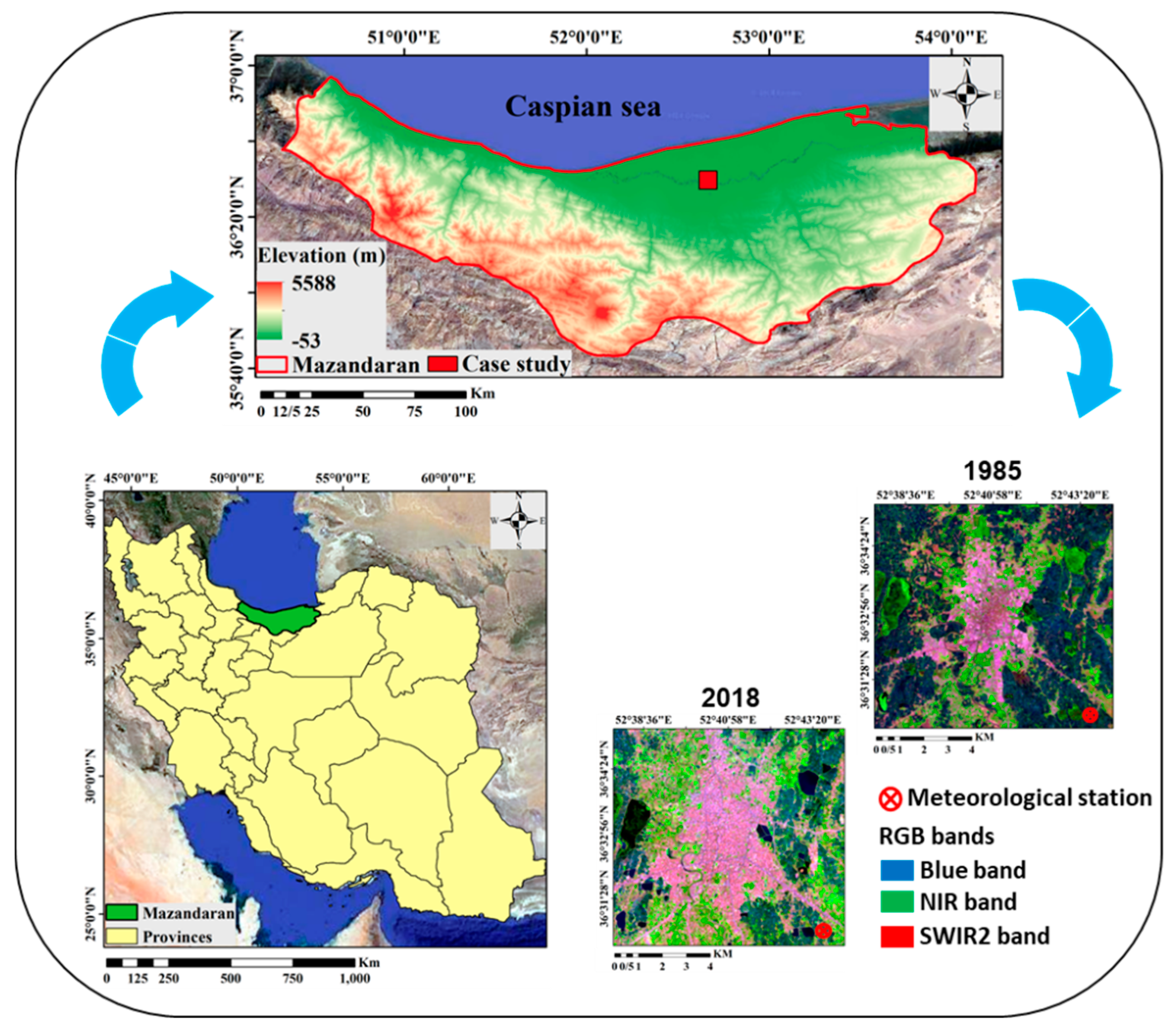
2. Study Area
3. Data and Methods
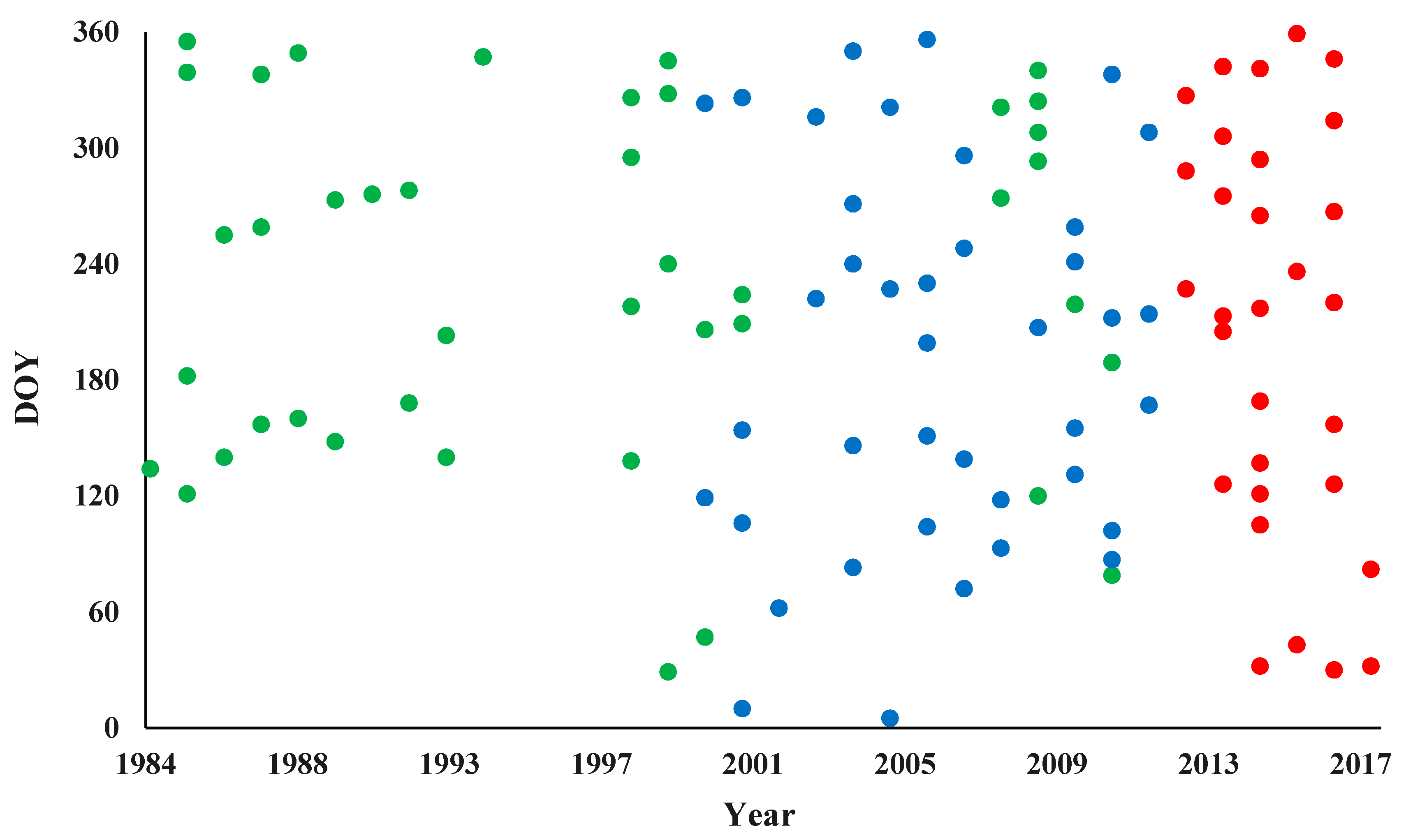
3.1. Data
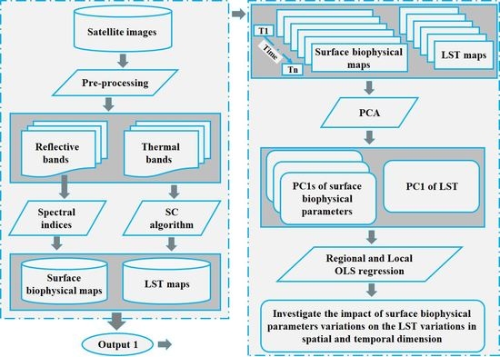
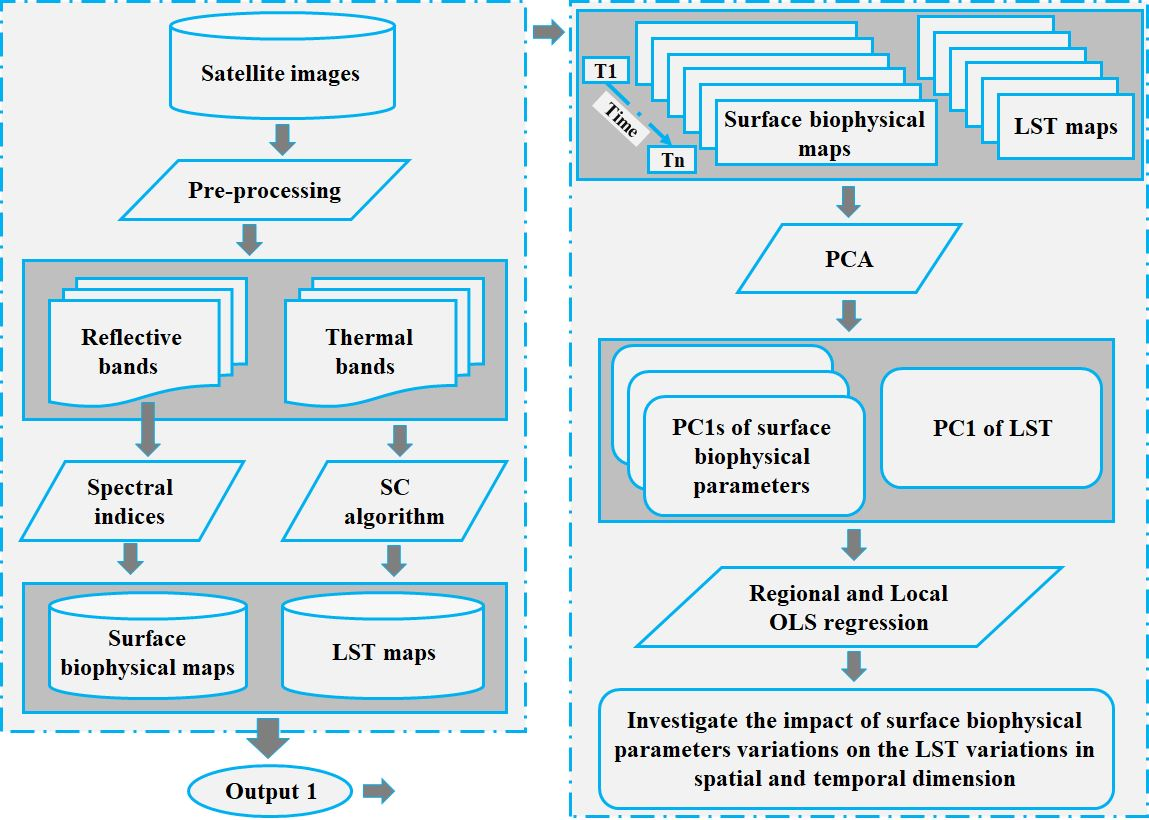
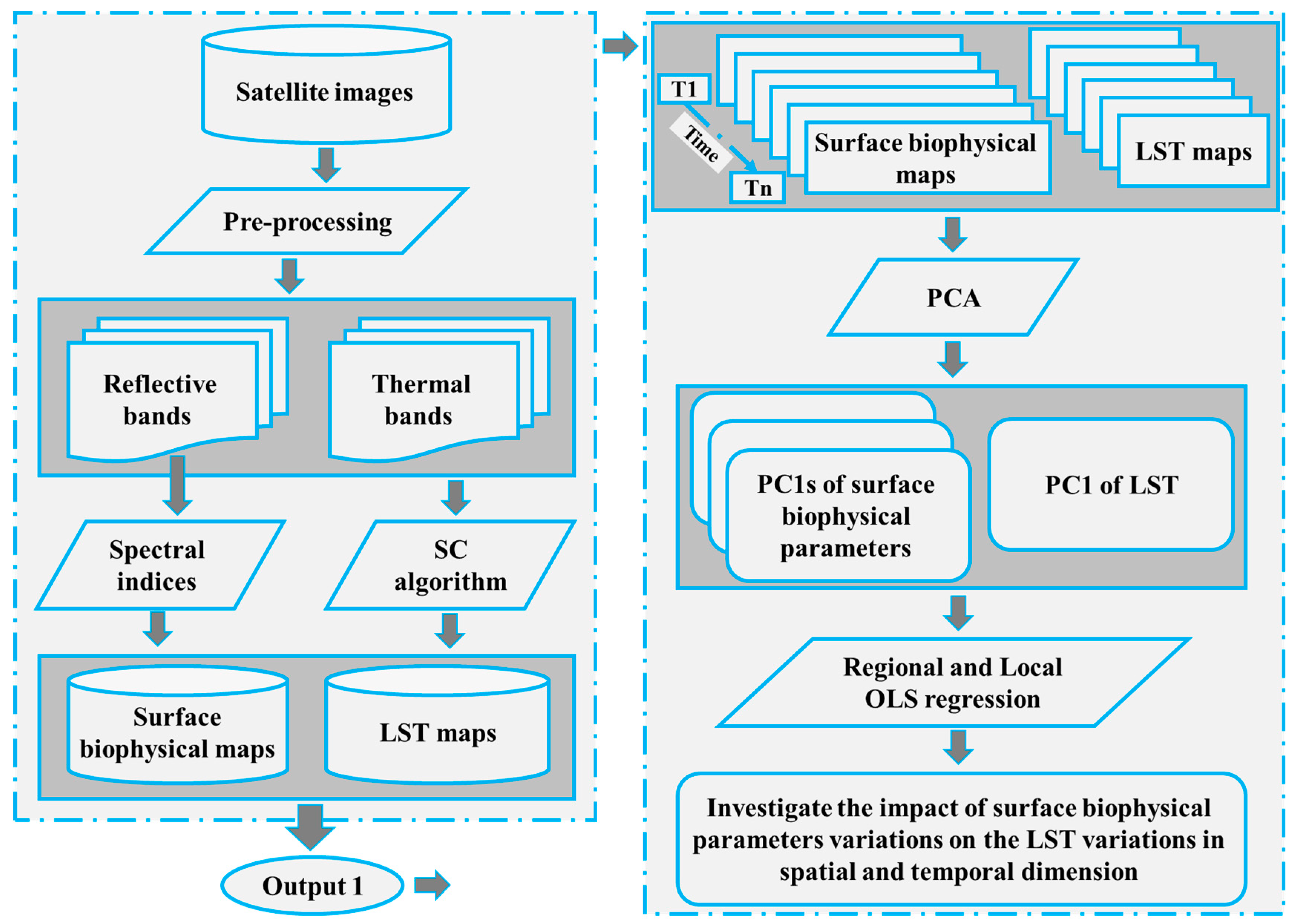
3.2. Methods
3.2.1. Image Preprocessing
3.2.2. LST and Surface Biophysical Parameters
3.2.3. LST and Surface Biophysical Parameters Variations
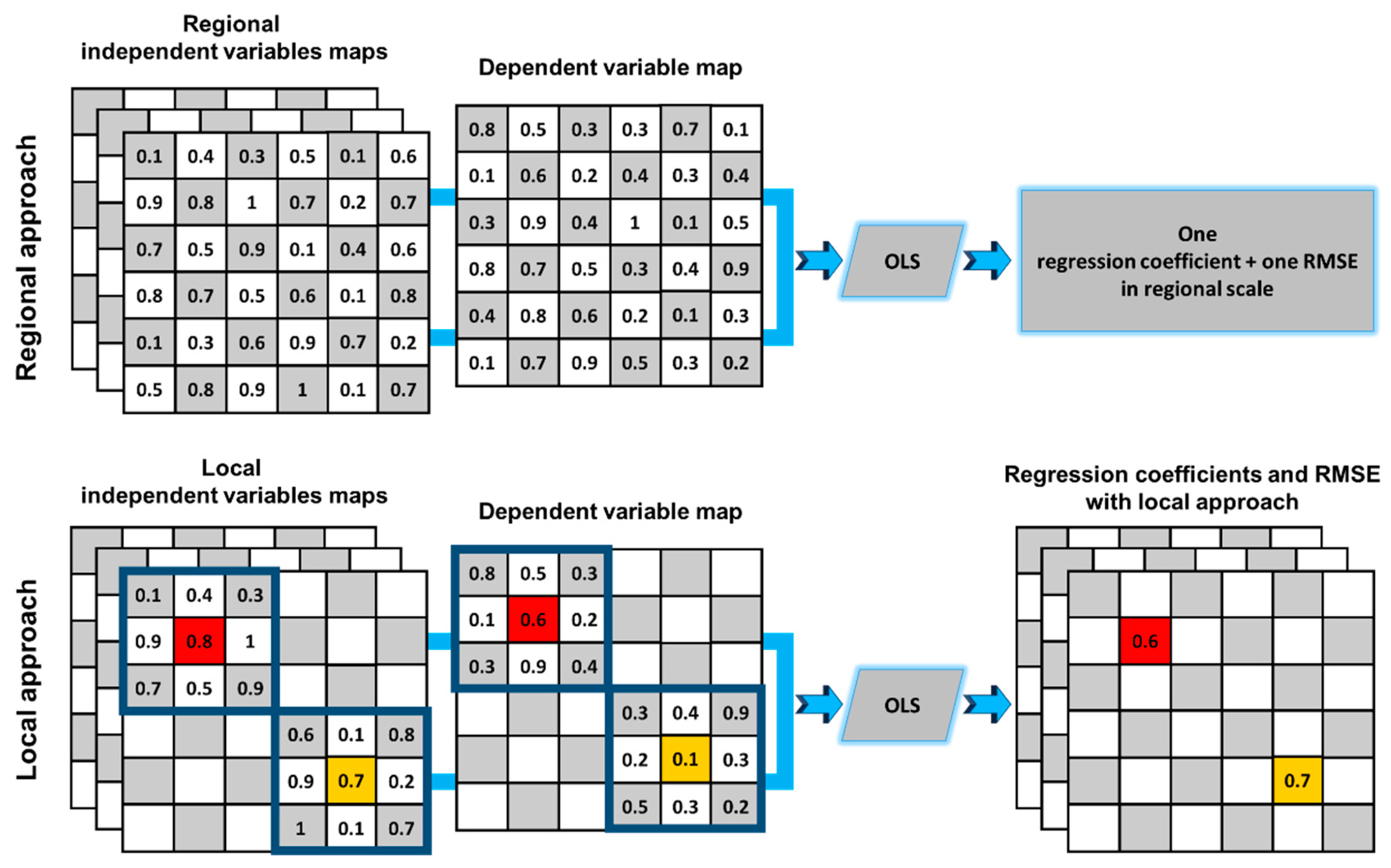
3.2.4. Impact of Surface Biophysical Parameter Variations on LST Variations
Regional and Local Optimization
3.2.5. Modeled LST Variations Based on Multivariate OLS Regression
4. Results
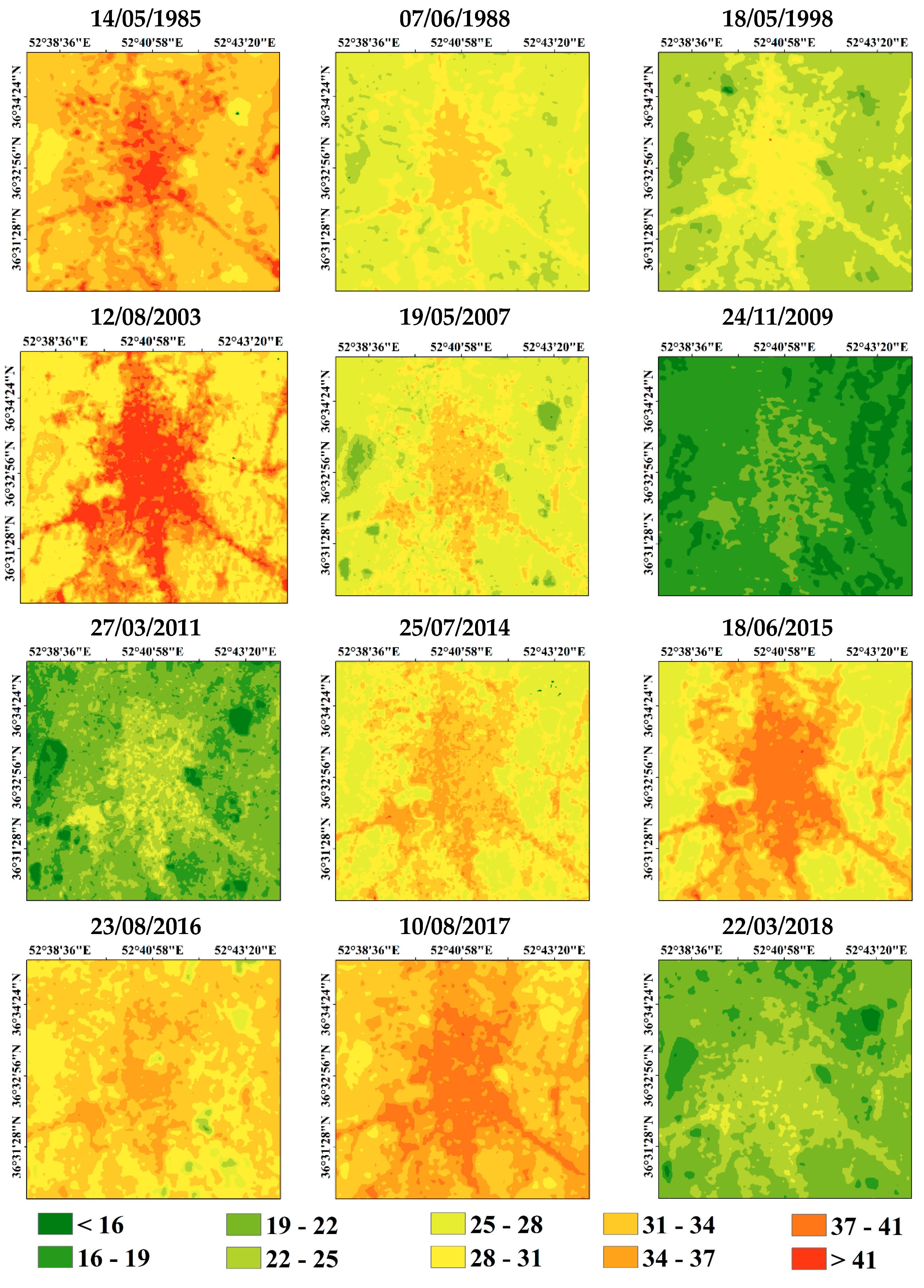
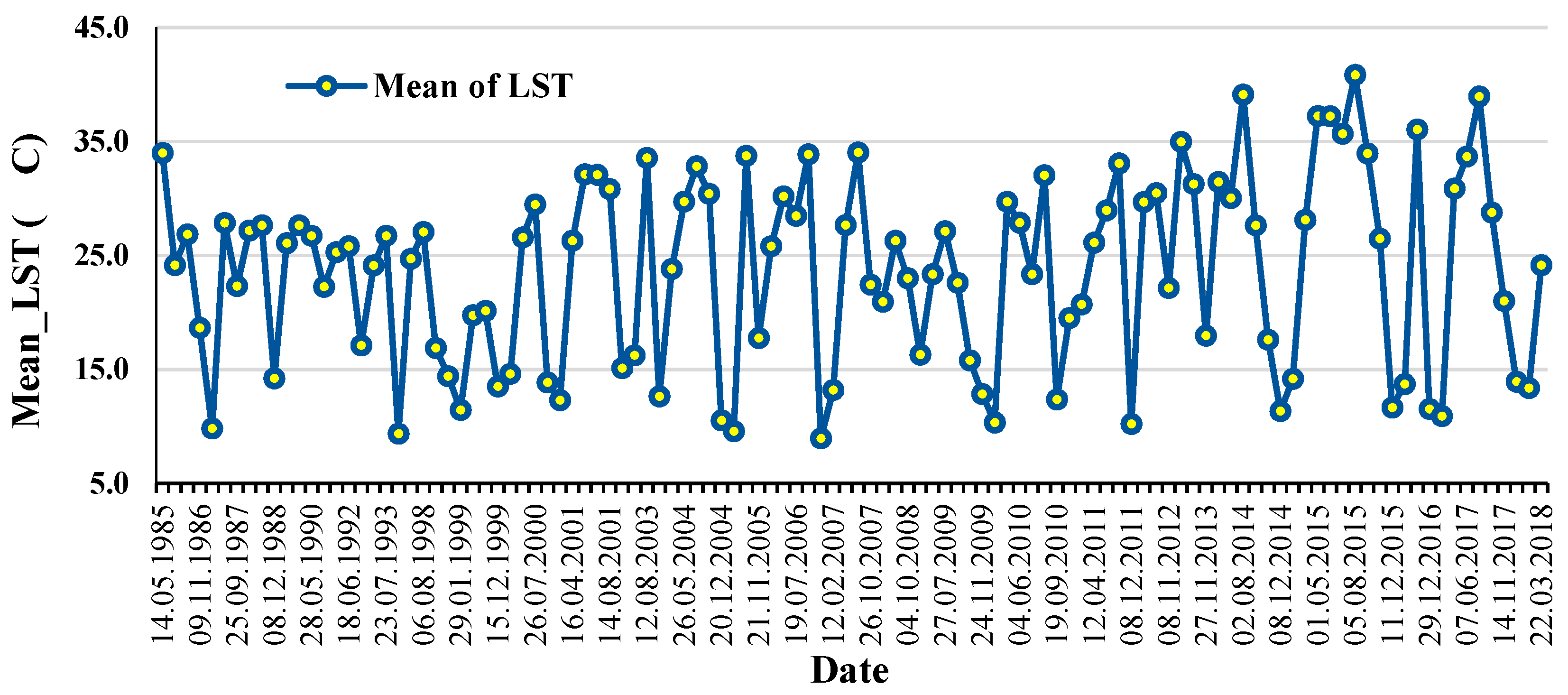
4.1. LST and Surface Biophysical Parameters
4.2. LST and Surface Biophysical Parameters Variations
4.3. Impact of Surface Biophysical Parameters Variations on LST Variations
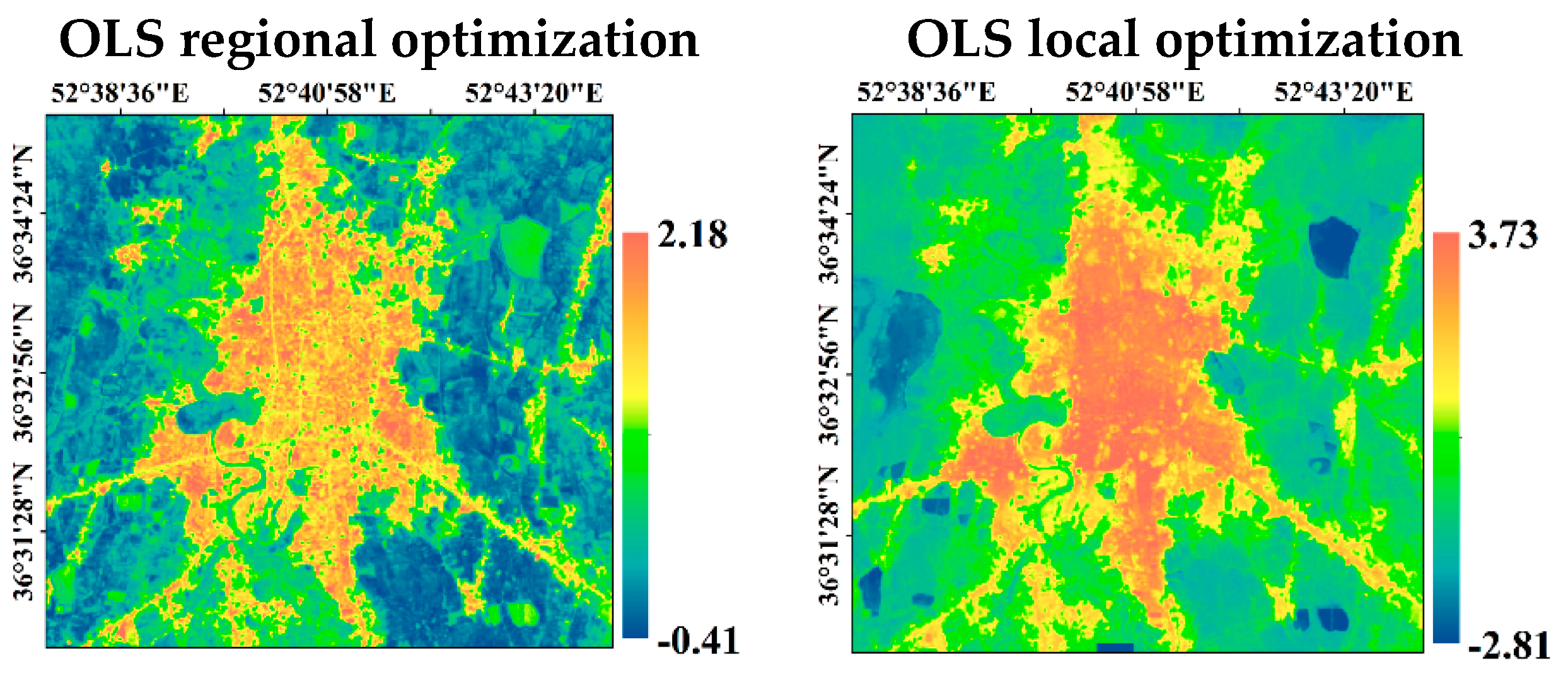
4.3.1. Regional Optimization
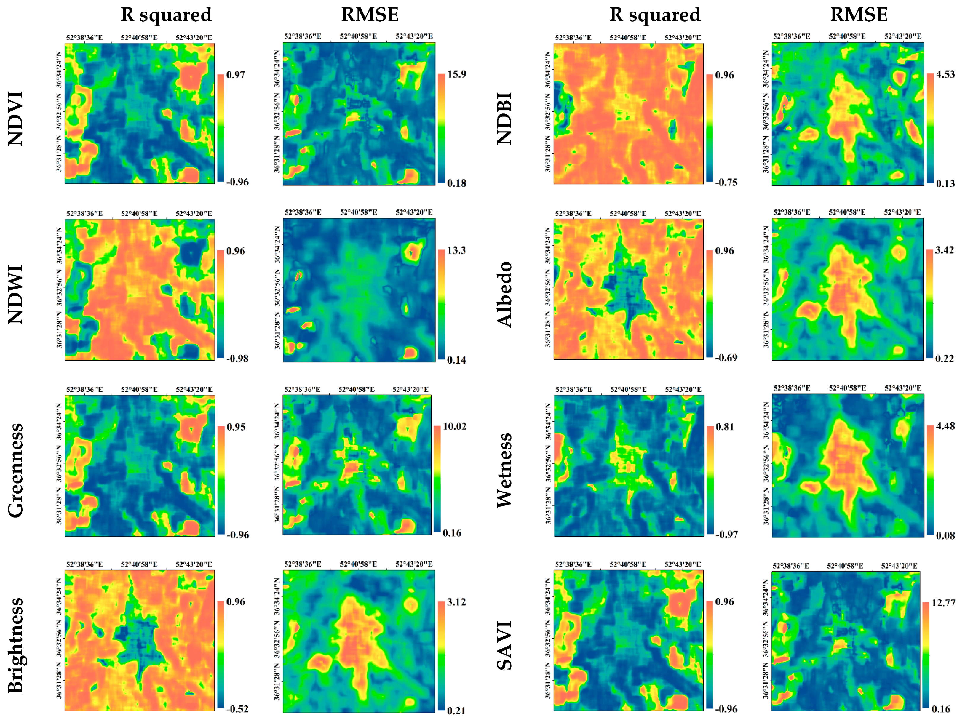
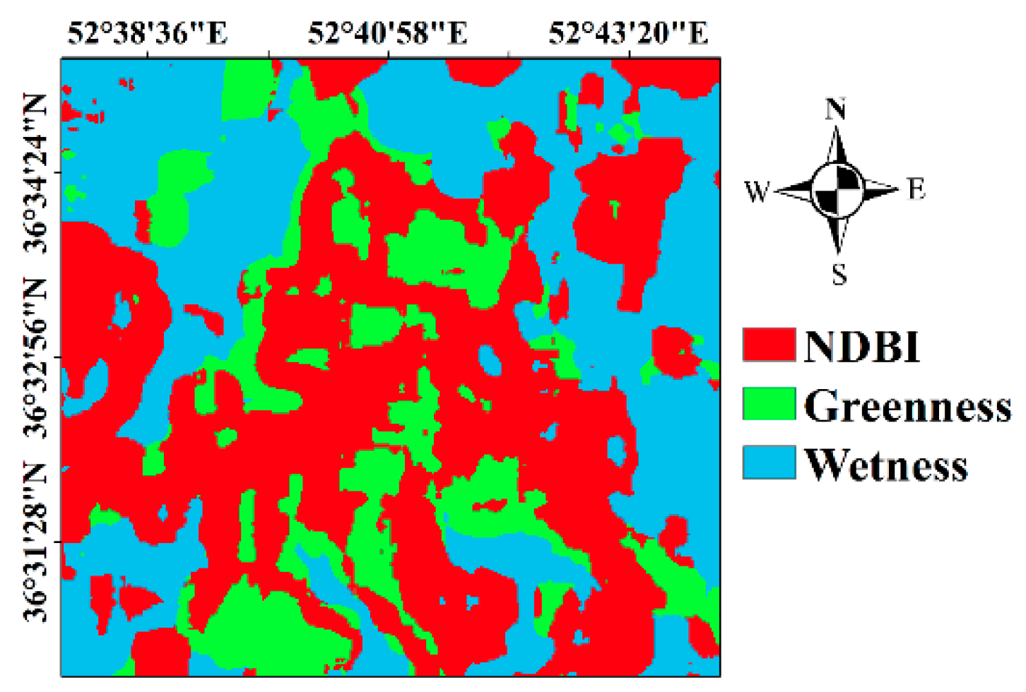
4.3.2. Local Optimization
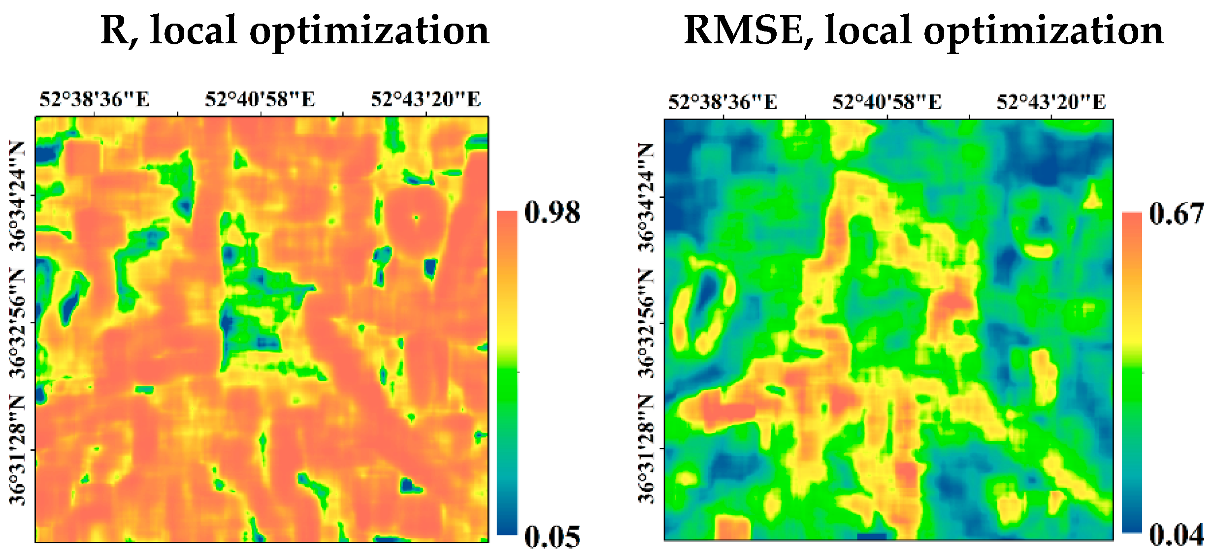
4.4. Modeled LST Variations Based on Multivariate OLS Regression
5. Discussion
6. Conclusions
Author Contributions
Funding
Acknowledgments
Conflicts of Interest
References
- Anderson, M.; Norman, J.; Kustas, W.; Houborg, R.; Starks, P.; Agam, N. A thermal-based remote sensing technique for routine mapping of land-surface carbon, water and energy fluxes from field to regional scales. Remote Sens. Environ. 2008, 112, 4227–4241. [Google Scholar] [CrossRef]
- Weng, Q.; Firozjaei, M.K.; Kiavarz, M.; Alavipanah, S.K.; Hamzeh, S. Normalizing land surface temperature for environmental parameters in mountainous and urban areas of a cold semi-arid climate. Sci. Total Environ. 2019, 650, 515–529. [Google Scholar] [CrossRef] [PubMed]
- Zhao, W.; Duan, S.-B.; Li, A.; Yin, G. A practical method for reducing terrain effect on land surface temperature using random forest regression. Remote Sens. Environ. 2019, 221, 635–649. [Google Scholar] [CrossRef]
- Long, D.; Singh, V.P. A two-source trapezoid model for evapotranspiration (ttme) from satellite imagery. Remote Sens. Environ. 2012, 121, 370–388. [Google Scholar] [CrossRef]
- Jiang, Y.; Weng, Q. Estimation of hourly and daily evapotranspiration and soil moisture using downscaled lst over various urban surfaces. GISci. Remote Sens. 2017, 54, 95–117. [Google Scholar] [CrossRef]
- Weng, Q. Thermal infrared remote sensing for urban climate and environmental studies: Methods, applications, and trends. ISPRS J. Photogramm. Remote Sens. 2009, 64, 335–344. [Google Scholar] [CrossRef]
- Weng, Q.; Lu, D.; Schubring, J. Estimation of land surface temperature—Vegetation abundance relationship for urban heat island studies. Remote Sens. Environ. 2004, 89, 467–483. [Google Scholar] [CrossRef]
- Firozjaei, M.K.; Kiavarz, M.; Alavipanah, S.K.; Lakes, T.; Qureshi, S. Monitoring and forecasting heat island intensity through multi-temporal image analysis and cellular automata-markov chain modelling: A case of babol city, iran. Ecol. Indic. 2018, 91, 155–170. [Google Scholar] [CrossRef]
- Leng, P.; Song, X.; Duan, S.-B.; Li, Z.-L. A practical algorithm for estimating surface soil moisture using combined optical and thermal infrared data. Int. J. Appl. Earth Obs. 2016, 52, 338–348. [Google Scholar] [CrossRef]
- Vlassova, L.; Pérez-Cabello, F.; Mimbrero, M.R.; Llovería, R.M.; García-Martín, A. Analysis of the relationship between land surface temperature and wildfire severity in a series of landsat images. Remote Sens. 2014, 6, 6136–6162. [Google Scholar] [CrossRef]
- Zhou, X.; Wang, Y.C. Dynamics of land surface temperature in response to land-use/cover change. Geogr. Res. 2011, 49, 23–36. [Google Scholar] [CrossRef]
- Guo, G.; Wu, Z.; Xiao, R.; Chen, Y.; Liu, X.; Zhang, X. Impacts of urban biophysical composition on land surface temperature in urban heat island clusters. Landsc. Urban Plan. 2015, 135, 1–10. [Google Scholar] [CrossRef]
- Ghosh, A.; Joshi, P. Hyperspectral imagery for disaggregation of land surface temperature with selected regression algorithms over different land use land cover scenes. ISPRS J. Photogramm. Remote Sens. 2014, 96, 76–93. [Google Scholar] [CrossRef]
- Malbéteau, Y.; Merlin, O.; Gascoin, S.; Gastellu, J.-P.; Mattar, C.; Olivera-Guerra, L.; Khabba, S.; Jarlan, L. Normalizing land surface temperature data for elevation and illumination effects in mountainous areas: A case study using aster data over a steep-sided valley in morocco. Remote Sens. Environ. 2017, 189, 25–39. [Google Scholar] [CrossRef]
- Jiang, J.; Tian, G. Analysis of the impact of land use/land cover change on land surface temperature with remote sensing. Procedia Environ. Sci. 2010, 2, 571–575. [Google Scholar] [CrossRef]
- Choudhury, D.; Das, K.; Das, A. Assessment of land use land cover changes and its impact on variations of land surface temperature in asansol-durgapur development region. Egypt. J. Remote Sens. Space Sci. 2019, 22, 203–218. [Google Scholar] [CrossRef]
- Son, N.; Chen, C.; Chen, C.; Chang, L.; Minh, V. Monitoring agricultural drought in the lower mekong basin using modis ndvi and land surface temperature data. Int. J. Appl. Earth Obs. 2012, 18, 417–427. [Google Scholar] [CrossRef]
- Xie, S.-P.; Deser, C.; Vecchi, G.A.; Ma, J.; Teng, H.; Wittenberg, A.T. Global warming pattern formation: Sea surface temperature and rainfall. J. Clim. 2010, 23, 966–986. [Google Scholar] [CrossRef]
- Weng, Q.; Firozjaei, M.K.; Sedighi, A.; Kiavarz, M.; Alavipanah, S.K. Statistical analysis of surface urban heat island intensity variations: A case study of babol city, iran. GISci. Remote Sens. 2019, 56, 576–604. [Google Scholar] [CrossRef]
- Giridharan, R.; Emmanuel, R. The impact of urban compactness, comfort strategies and energy consumption on tropical urban heat island intensity: A review. Sustain. Cities Soc. 2018, 40, 677–687. [Google Scholar] [CrossRef] [Green Version]
- Van Hove, L.; Jacobs, C.; Heusinkveld, B.; Elbers, J.; Van Driel, B.; Holtslag, A. Temporal and spatial variability of urban heat island and thermal comfort within the rotterdam agglomeration. Build. Environ. 2015, 83, 91–103. [Google Scholar] [CrossRef]
- Xiao, H.; Weng, Q. The impact of land use and land cover changes on land surface temperature in a karst area of china. J. Environ. Manag. 2007, 85, 245–257. [Google Scholar] [CrossRef] [PubMed]
- Li, H.; Liu, Q.-H.; Zou, J. Relationships of LST to NDBI and NDVI in changsha-zhuzhou-xiangtan area based on MODIS data. Sci. Geogr. Sin. 2009, 2, 018. [Google Scholar]
- Zakšek, K.; Oštir, K. Downscaling land surface temperature for urban heat island diurnal cycle analysis. Remote Sens. Environ. 2012, 117, 114–124. [Google Scholar] [CrossRef]
- Keramitsoglou, I.; Kiranoudis, C.T.; Weng, Q. Downscaling geostationary land surface temperature imagery for urban analysis. IEEE Geosci. Remote Sens. Lett. 2013, 10, 1253–1257. [Google Scholar] [CrossRef]
- Maeda, E.E. Downscaling modis lst in the east african mountains using elevation gradient and land-cover information. Int. J. Remote Sens. 2014, 35, 3094–3108. [Google Scholar] [CrossRef]
- Bisquert, M.; Sánchez, J.M.; Caselles, V. Evaluation of disaggregation methods for downscaling modis land surface temperature to landsat spatial resolution in barrax test site. IEEE J. Sel. Top. Appl. Earth Obs. Remote Sens. 2016, 9, 1430–1438. [Google Scholar] [CrossRef]
- Zhan, W.; Chen, Y.; Zhou, J.; Wang, J.; Liu, W.; Voogt, J.; Zhu, X.; Quan, J.; Li, J. Disaggregation of remotely sensed land surface temperature: Literature survey, taxonomy, issues, and caveats. Remote Sens. Environ. 2013, 131, 119–139. [Google Scholar] [CrossRef]
- Hutengs, C.; Vohland, M. Downscaling land surface temperatures at regional scales with random forest regression. Remote Sens. Environ. 2016, 178, 127–141. [Google Scholar] [CrossRef]
- Sismanidis, P.; Keramitsoglou, I.; Bechtel, B.; Kiranoudis, C. Improving the downscaling of diurnal land surface temperatures using the annual cycle parameters as disaggregation kernels. Remote Sens. 2016, 9, 23. [Google Scholar] [CrossRef]
- He, J.; Zhao, W.; Li, A.; Wen, F.; Yu, D. The impact of the terrain effect on land surface temperature variation based on landsat-8 observations in mountainous areas. Int. J. Remote Sens. 2018, 40, 1808–1827. [Google Scholar] [CrossRef]
- Yang, Y.; Cao, C.; Pan, X.; Li, X.; Zhu, X. Downscaling land surface temperature in an arid area by using multiple remote sensing indices with random forest regression. Remote Sens. 2017, 9, 789. [Google Scholar] [CrossRef]
- Sattari, F.; Hashim, M.; Pour, A.B. Thermal sharpening of land surface temperature maps based on the impervious surface index with the tsharp method to aster satellite data: A case study from the metropolitan kuala lumpur, malaysia. Measurement 2018, 125, 262–278. [Google Scholar] [CrossRef]
- Jeganathan, C.; Hamm, N.; Mukherjee, S.; Atkinson, P.M.; Raju, P.; Dadhwal, V. Evaluating a thermal image sharpening model over a mixed agricultural landscape in india. Int. J. Appl. Earth Obs. 2011, 13, 178–191. [Google Scholar] [CrossRef]
- Gao, F.; Kustas, W.; Anderson, M. A data mining approach for sharpening thermal satellite imagery over land. Remote Sens. 2012, 4, 3287–3319. [Google Scholar] [CrossRef]
- Wang, F.; Qin, Z.; Li, W.; Song, C.; Karnieli, A.; Zhao, S. An efficient approach for pixel decomposition to increase the spatial resolution of land surface temperature images from modis thermal infrared band data. Sensors 2015, 15, 304–330. [Google Scholar] [CrossRef]
- Eklundh, L.; Singh, A. A comparative analysis of standardised and unstandardised principal components analysis in remote sensing. Int. J. Remote Sens. 1993, 14, 1359–1370. [Google Scholar] [CrossRef]
- Henebry, G.M.; Rieck, D.R. Applying principal components analysis to image time series: Effects on scene segmentation and spatial structure. In Proceedings of the IGARSS’96. 1996 International Geoscience and Remote Sensing Symposium, Lincoln, NE, USA, 31–31 May 1996; pp. 448–450. [Google Scholar]
- Singh, A.; Harrison, A. Standardized principal components. Int. J. Remote Sens. 1985, 6, 883–896. [Google Scholar] [CrossRef]
- Jensen, J.R. Introductory Digital Image Processing: A Remote Sensing Perspective; Prentice Hall Press: Upper Saddle River, NJ, USA, 2015. [Google Scholar]
- Jolliffe, I.T.; Cadima, J. Principal component analysis: A review and recent developments. Philos. Trans. R. Soc. A Math. Phys. Eng. Sci. 2016, 374, 20150202. [Google Scholar] [CrossRef]
- Deng, J.; Huang, Y.; Chen, B.; Tong, C.; Liu, P.; Wang, H.; Hong, Y. A methodology to monitor urban expansion and green space change using a time series ofmulti-sensor spot and sentinel-2a images. Remote Sens. 2019, 11, 1230. [Google Scholar] [CrossRef]
- Eastman, J.R.; Fulk, M. Long sequence time series evaluation using standardized principal components. Photogramm. Eng. Remote Sens. 1993, 59, 1307–1312. [Google Scholar]
- Hall-Beyer, M. Comparison of single-year and multiyear ndvi time series principal components in cold temperate biomes. IEEE Trans. Geosci. Remote Sens. 2003, 41, 2568–2574. [Google Scholar] [CrossRef] [Green Version]
- Bellón, B.; Bégué, A.; Lo Seen, D.; de Almeida, C.; Simões, M. A remote sensing approach for regional-scale mapping of agricultural land-use systems based on ndvi time series. Remote Sens. 2017, 9, 600. [Google Scholar] [CrossRef]
- Hirosawa, Y.; Marsh, S.E.; Kliman, D.H. Application of standardized principal component analysis to land-cover characterization using multitemporal avhrr data. Remote Sens. Environ. 1996, 58, 267–281. [Google Scholar] [CrossRef]
- Wang, T.; Kou, X.; Xiong, Y.; Mou, P.; Wu, J.; Ge, J. Temporal and spatial patterns of ndvi and their relationship to precipitation in the loess plateau of china. Int. J. Remote Sens. 2010, 31, 1943–1958. [Google Scholar] [CrossRef]
- De Almeida, T.I.R.; Penatti, N.C.; Ferreira, L.G.; Arantes, A.E.; do Amaral, C.H. Principal component analysis applied to a time series of modis images: The spatio-temporal variability of the pantanal wetland, brazil. Wetl. Ecol. Manag. 2015, 23, 737–748. [Google Scholar] [CrossRef]
- Deng, J.; Wang, K.; Deng, Y.; Qi, G. Pca-based land-use change detection and analysis using multitemporal and multisensor satellite data. Int. J. Remote Sens. 2008, 29, 4823–4838. [Google Scholar] [CrossRef]
- Panah, S.; Mogaddam, M.K.; Firozjaei, M.K. Monitoring spatiotemporal changes of heat island in babol city due to land use changes. Int. Arch. Photogramm. Remote Sens. Spat. Inf. Sci. 2017, 42, 17–22. [Google Scholar] [CrossRef]
- Firozjaei, M.K.; Sedighi, A.; Argany, M.; Jelokhani-Niaraki, M.; Arsanjani, J.J. A geographical direction-based approach for capturing the local variation of urban expansion in the application of CA-Markov model. Cities 2019, 93, 120–135. [Google Scholar] [CrossRef]
- USGS. United States Geological Survey. Available online: https://earthexplorer.usgs.gov/ (accessed on 1 June 2018).
- LAADS DAAC. Level-1 and Atmosphere Archive and Distribution System Distributed Active Archive Center. Available online: https://ladsweb.nascom.nasa.gov (accessed on 1 June 2018).
- Mazandaran Meteorological Organization. Available online: http://www.Mazmet.Ir/en (accessed on 1 June 2018).
- Berk, A.; Conforti, P.; Kennett, R.; Perkins, T.; Hawes, F.; van den Bosch, J. Modtran® 6: A major upgrade of the modtran® radiative transfer code. In Proceedings of the 2014 6th Workshop on Hyperspectral Image and Signal Processing: Evolution in Remote Sensing (WHISPERS), Lausanne, Switzerland, 24–27 June 2014; pp. 1–4. [Google Scholar]
- Chander, G.; Markham, B.L.; Helder, D.L. Summary of current radiometric calibration coefficients for landsat mss, tm, etm+, and eo-1 ali sensors. Remote Sens. Environ. 2009, 113, 893–903. [Google Scholar] [CrossRef]
- Mishra, N.; Haque, M.O.; Leigh, L.; Aaron, D.; Helder, D.; Markham, B. Radiometric cross calibration of landsat 8 operational land imager (oli) and landsat 7 enhanced thematic mapper plus (etm+). Remote Sens. 2014, 6, 12619–12638. [Google Scholar] [CrossRef]
- Moghaddam, M.H.R.; Sedighi, A.; Fasihi, S.; Firozjaei, M.K. Effect of environmental policies in combating aeolian desertification over sejzy plain of iran. Aeolian Res. 2018, 35, 19–28. [Google Scholar] [CrossRef]
- Arvidson, T.; Goward, S.; Gasch, J.; Williams, D. Landsat-7 long-term acquisition plan. Photogramm. Eng. Remote Sens. 2006, 72, 1137–1146. [Google Scholar] [CrossRef]
- Chen, J.; Zhu, X.; Vogelmann, J.E.; Gao, F.; Jin, S. A simple and effective method for filling gaps in landsat etm+ slc-off images. Remote Sens. Environ. 2011, 115, 1053–1064. [Google Scholar] [CrossRef]
- Yu, X.; Guo, X.; Wu, Z. Land surface temperature retrieval from landsat 8 tirs—Comparison between radiative transfer equation-based method, split window algorithm and single channel method. Remote Sens. 2014, 6, 9829–9852. [Google Scholar] [CrossRef]
- Jimenez-Munoz, J.C.; Sobrino, J.A.; Skokovic, D.; Mattar, C.; Cristobal, J. Land surface temperature retrieval methods from landsat-8 thermal infrared sensor data. IEEE Geosci. Remote Sens. Lett. 2014, 11, 1840–1843. [Google Scholar] [CrossRef]
- Barsi, J.A.; Schott, J.R.; Hook, S.J.; Raqueno, N.G.; Markham, B.L.; Radocinski, R.G. Landsat-8 thermal infrared sensor (tirs) vicarious radiometric calibration. Remote Sens. 2014, 6, 11607–11626. [Google Scholar] [CrossRef]
- Jiménez-Muñoz, J.C.; Sobrino, J.A. A generalized single-channel method for retrieving land surface temperature from remote sensing data. J. Geophys. Res. Atmos. 2003, 108. [Google Scholar] [CrossRef]
- Sobrino, J.A.; Jiménez-Muñoz, J.C.; Sòria, G.; Romaguera, M.; Guanter, L.; Moreno, J.; Plaza, A.; Martínez, P. Land surface emissivity retrieval from different vnir and tir sensors. IEEE Trans. Geosci. Remote Sens. 2008, 46, 316–327. [Google Scholar] [CrossRef]
- Tucker, C.J. Red and photographic infrared linear combinations for monitoring vegetation. Remote Sens. Environ. 1979, 8, 127–150. [Google Scholar] [CrossRef] [Green Version]
- Huete, A.R. A soil-adjusted vegetation index (savi). Remote Sens. Environ. 1988, 25, 295–309. [Google Scholar] [CrossRef]
- Gao, B.-C. Ndwi—A normalized difference water index for remote sensing of vegetation liquid water from space. Remote Sens. Environ. 1996, 58, 257–266. [Google Scholar] [CrossRef]
- Zha, Y.; Gao, J.; Ni, S. Use of normalized difference built-up index in automatically mapping urban areas from tm imagery. Int. J. Remote Sens. 2003, 24, 583–594. [Google Scholar] [CrossRef]
- Liang, S. Narrowband to broadband conversions of land surface albedo i: Algorithms. Remote Sens. Environ. 2001, 76, 213–238. [Google Scholar] [CrossRef]
- Silva, B.B.D.; Braga, A.C.; Braga, C.C.; de Oliveira, L.M.; Montenegro, S.M.; Barbosa Junior, B. Procedures for calculation of the albedo with oli-landsat 8 images: Application to the brazilian semi-arid. Rev. Bras. Eng. Agrícola Ambient. 2016, 20, 3–8. [Google Scholar] [CrossRef]
- Huang, C.; Wylie, B.; Yang, L.; Homer, C.; Zylstra, G. Derivation of a tasselled cap transformation based on landsat 7 at-satellite reflectance. Int. J. Remote Sens. 2002, 23, 1741–1748. [Google Scholar] [CrossRef]
- Liu, Q.; Liu, G.; Huang, C.; Liu, S.; Zhao, J. A tasseled cap transformation for landsat 8 oli toa reflectance images. In Proceedings of the 2014 IEEE International Geoscience and Remote Sensing Symposium (IGARSS), Quebec City, QC, Canada, 13–18 July 2014; pp. 541–544. [Google Scholar]
- Liu, Q.; Liu, G.; Huang, C.; Xie, C. Comparison of tasselled cap transformations based on the selective bands of landsat 8 oli toa reflectance images. Int. J. Remote Sens. 2015, 36, 417–441. [Google Scholar] [CrossRef]
- Dalal, S.; Shirodkar, P.; Jagtap, T.; Naik, B.; Rao, G. Evaluation of significant sources influencing the variation of water quality of kandla creek, gulf of katchchh, using pca. Environ. Monit. Assess. 2010, 163, 49–56. [Google Scholar] [CrossRef]
- Vukovich, F.M.; Sherwell, J. An examination of the relationship between certain meteorological parameters and surface ozone variations in the baltimore–washington corridor. Atmos. Environ. 2003, 37, 971–981. [Google Scholar] [CrossRef]
- Ouyang, Y.; Nkedi-Kizza, P.; Wu, Q.; Shinde, D.; Huang, C. Assessment of seasonal variations in surface water quality. Water Res. 2006, 40, 3800–3810. [Google Scholar] [CrossRef]
- Mas, J.-F. Monitoring land-cover changes: A comparison of change detection techniques. Int. J. Remote Sens. 1999, 20, 139–152. [Google Scholar] [CrossRef]
- Gaitani, N.; Burud, I.; Thiis, T.; Santamouris, M. High-resolution spectral mapping of urban thermal properties with unmanned aerial vehicles. Build. Environ. 2017, 121, 215–224. [Google Scholar] [CrossRef]
- Vázquez-Jiménez, R.; Ramos-Bernal, R.N.; Romero-Calcerrada, R.; Arrogante-Funes, P.; Tizapa, S.S.; Novillo, C.J. Thresholding algorithm optimization for change detection to satellite imagery. In Colorimetry and Image Processing; IntechOpen: Gran Canaria, Spain, 2017. [Google Scholar]
- Weng, Q.; Rajasekar, U.; Hu, X. Modeling urban heat islands and their relationship with impervious surface and vegetation abundance by using aster images. IEEE Trans. Geosci. Remote Sens. 2011, 49, 4080–4089. [Google Scholar] [CrossRef]
- Jolliffe, I. Principal Component Analysis; Springer: Berlin/Heidelberg, Germany, 2011. [Google Scholar]
- Hutcheson, G.D. Ordinary least-squares regression. In The SAGE Dictionary of Quantitative Management Research; Moutinho, L., Hutcheson, G.D., Eds.; Sage: London, UK, 2011; pp. 224–228. [Google Scholar]
- Yang, Y.; Li, X.; Pan, X.; Zhang, Y.; Cao, C. Downscaling land surface temperature in complex regions by using multiple scale factors with adaptive thresholds. Sensors 2017, 17, 744. [Google Scholar] [CrossRef] [PubMed]
- Srivastava, P.K.; Majumdar, T.; Bhattacharya, A.K. Surface temperature estimation in singhbhum shear zone of india using landsat-7 etm+ thermal infrared data. Adv. Space Res. 2009, 43, 1563–1574. [Google Scholar] [CrossRef]
- Qin, Q.; Zhang, N.; Nan, P.; Chai, L. Geothermal area detection using landsat etm+ thermal infrared data and its mechanistic analysis—A case study in Tengchong, China. Int. J. Appl. Earth Obs. 2011, 13, 552–559. [Google Scholar] [CrossRef]
- Firozjaei, M.K.; Kiavarz, M.; Nematollahi, O.; Karimpour Reihan, M.; Alavipanah, S.K. An evaluation of energy balance parameters, and the relations between topographical and biophysical characteristics using the mountainous surface energy balance algorithm for land (SEBAL). Int. J. Remote Sens. 2019, 40, 5230–5260. [Google Scholar] [CrossRef]
- Bindhu, V.; Narasimhan, B.; Sudheer, K. Development and verification of a non-linear disaggregation method (nl-distrad) to downscale modis land surface temperature to the spatial scale of landsat thermal data to estimate evapotranspiration. Remote Sens. Environ. 2013, 135, 118–129. [Google Scholar] [CrossRef]
- Allen, R.G.; Trezza, R.; Tasumi, M. Analytical integrated functions for daily solar radiation on slopes. Agric. For. Meteorol. 2006, 139, 55–73. [Google Scholar] [CrossRef]
- Kalogirou, S.A. Solar Energy Engineering: Processes and Systems; Academic Press: Cambridge, MA, USA, 2013. [Google Scholar]
- Zhao, W.; Wu, H.; Yin, G.; Duan, S.-B. Normalization of the temporal effect on the modis land surface temperature product using random forest regression. ISPRS J. Photogramm. Remote Sens. 2019, 152, 109–118. [Google Scholar] [CrossRef]
- Abdel-Rahman, E.M.; Ahmed, F.B.; Ismail, R. Random forest regression and spectral band selection for estimating sugarcane leaf nitrogen concentration using eo-1 hyperion hyperspectral data. Int. J. Remote Sens. 2013, 34, 712–728. [Google Scholar] [CrossRef]
- Noi, P.T.; Degener, J.; Kappas, M. Comparison of multiple linear regression, cubist regression, and random forest algorithms to estimate daily air surface temperature from dynamic combinations of modis lst data. Remote Sens. 2017, 9, 398. [Google Scholar] [CrossRef]
- Strobl, C.; Malley, J.; Tutz, G. An introduction to recursive partitioning: Rationale, application, and characteristics of classification and regression trees, bagging, and random forests. Psychol. Methods 2009, 14, 323–348. [Google Scholar] [CrossRef] [PubMed]


| Biophysical Parameter | Description | References |
|---|---|---|
| NDVI | [66] | |
| SAVI | [67] | |
| NDWI | [68] | |
| NDBI | [69] | |
| Brightness | 0.3029Blue + 0.2786Green + 0.4733Red + 0.5599NIR + 0.5080SWIR1 + (For Landsat 8) 0.1872SWIR2 | [72,73,74] |
| Greenness | −0.2941Blue − 0.243Green − 0.5424Red + 0.7276NIR + (For Landsat 8) 0.0713SWIR1 − 0.1608SWIR2 | |
| Wetness | 0.1511Blue + 0.1973Green + 0.3283Red + 0.3407NIR − 0.7117SWIR1 − (For Landsat 8) 0.4559SWIR2 |
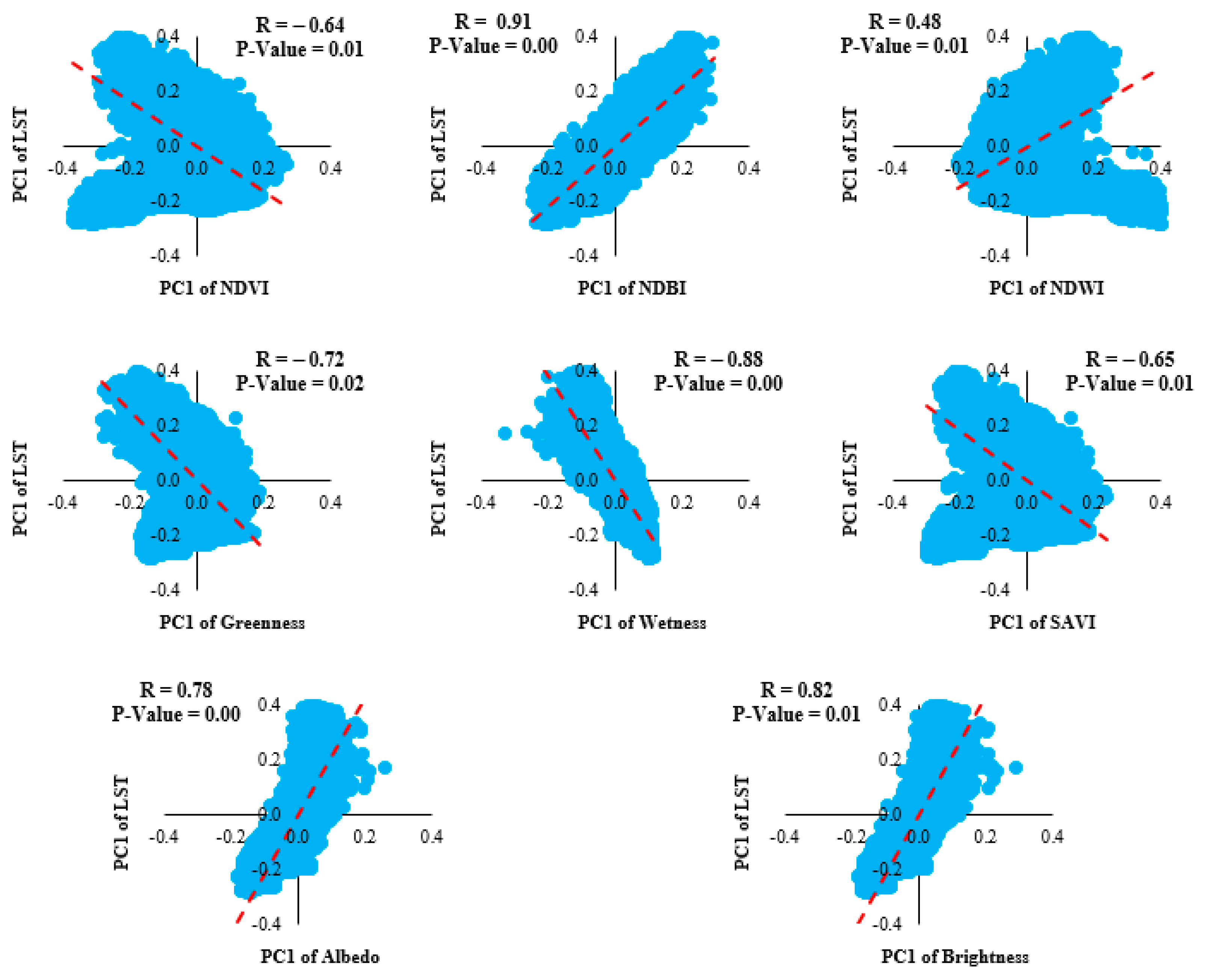
| Surface Biophysical Parameters | NDVI | NDBI | NDWI | Albedo | Greenness | Wetness | Brightness | SAVI |
|---|---|---|---|---|---|---|---|---|
| R squared | −0.44 | 0.71 | 0.29 | 0.58 | −0.57 | −0.68 | 0.63 | −0.46 |
| p-Value | 0.01 | 0.01 | 0.02 | 0.01 | 0.00 | 0.01 | 0.02 | 0.00 |
| Surface Biophysical Parameters | NDVI | NDBI | NDWI | Albedo | Greenness | Wetness | Brightness | SAVI |
|---|---|---|---|---|---|---|---|---|
| Mean value of R | −0.37 | 0.75 | 0.29 | 0.59 | −0.44 | −0.70 | 0.65 | −0.37 |
| Std of R | 0.50 | 0.22 | 0.54 | 0.30 | 0.48 | 0.25 | 0.26 | 0.30 |
| Mean value of RMSE | 1.15 | 0.71 | 1.17 | 1.05 | 1.06 | 1.03 | 1.05 | 1.15 |
| Std of RMSE | 0.95 | 0.32 | 0.95 | 0.48 | 0.77 | 0.87 | 0.49 | 0.91 |
© 2019 by the authors. Licensee MDPI, Basel, Switzerland. This article is an open access article distributed under the terms and conditions of the Creative Commons Attribution (CC BY) license (http://creativecommons.org/licenses/by/4.0/).
Share and Cite
Firozjaei, M.K.; Alavipanah, S.K.; Liu, H.; Sedighi, A.; Mijani, N.; Kiavarz, M.; Weng, Q. A PCA–OLS Model for Assessing the Impact of Surface Biophysical Parameters on Land Surface Temperature Variations. Remote Sens. 2019, 11, 2094. https://0-doi-org.brum.beds.ac.uk/10.3390/rs11182094
Firozjaei MK, Alavipanah SK, Liu H, Sedighi A, Mijani N, Kiavarz M, Weng Q. A PCA–OLS Model for Assessing the Impact of Surface Biophysical Parameters on Land Surface Temperature Variations. Remote Sensing. 2019; 11(18):2094. https://0-doi-org.brum.beds.ac.uk/10.3390/rs11182094
Chicago/Turabian StyleFirozjaei, Mohammad Karimi, Seyed Kazem Alavipanah, Hua Liu, Amir Sedighi, Naeim Mijani, Majid Kiavarz, and Qihao Weng. 2019. "A PCA–OLS Model for Assessing the Impact of Surface Biophysical Parameters on Land Surface Temperature Variations" Remote Sensing 11, no. 18: 2094. https://0-doi-org.brum.beds.ac.uk/10.3390/rs11182094