Article

Hourly PM2.5 Estimates from a Geostationary Satellite Based on an Ensemble Learning Algorithm and Their Spatiotemporal Patterns over Central East China

1
Laboratory of Environmental Model and Data Optima (EMDO), Laurel, MD 20707, USA
2
State Key Laboratory of Severe Weather, Beijing 100081, China
3
Earth System Science Interdisciplinary Center, University of Maryland, College Park, MD 20740, USA
4
Department of Atmospheric and Oceanic Science, University of Maryland, College Park, MD 20742, USA
*
Author to whom correspondence should be addressed.
Remote Sens. 2019, 11(18), 2120; https://0-doi-org.brum.beds.ac.uk/10.3390/rs11182120
Submission received: 23 July 2019 / Revised: 28 August 2019 / Accepted: 9 September 2019 / Published: 12 September 2019
(This article belongs to the Special Issue Remote Sensing of Greenhouse Gases and Air Pollution)

Abstract

:
Satellite-derived aerosol optical depths (AODs) have been widely used to estimate surface fine particulate matter (PM2.5) concentrations over areas that do not have PM2.5 monitoring sites. To date, most studies have focused on estimating daily PM2.5 concentrations using polar-orbiting satellite data (e.g., from the Moderate Resolution Imaging Spectroradiometer), which are inadequate for understanding the evolution of PM2.5 distributions. This study estimates hourly PM2.5 concentrations from Himawari AOD and meteorological parameters using an ensemble learning model. We analyzed the spatial agglomeration patterns of the estimated PM2.5 concentrations over central East China. The estimated PM2.5 concentrations agree well with ground-based data with an overall cross-validated coefficient of determination of 0.86 and a root-mean-square error of 17.3 μg m−3. Satellite-estimated PM2.5 concentrations over central East China display a north-to-south decreasing gradient with the highest concentration in winter and the lowest concentration in summer. Diurnally, concentrations are higher in the morning and lower in the afternoon. PM2.5 concentrations exhibit a significant spatial agglomeration effect in central East China. The errors in AOD do not necessarily affect the retrieval accuracy of PM2.5 proportionally, especially if the error is systematic. High-frequency spatiotemporal PM2.5 variations can improve our understanding of the formation and transportation processes of regional pollution episodes.

Graphical Abstract

1. Introduction

The concentration of atmospheric particulate matter with an aerodynamic diameter of less than 2.5 micrometers (PM2.5) is an important index of air pollution and has been widely used in epidemiological studies, such as the exposure response functions for health effects of air pollutants [1] and an assessment of mortality attributable to pollution [2]. PM2.5 has been reported to be strongly associated with cardiovascular diseases, public morbidity, and premature death (e.g., [3,4]). Studies on PM2.5 have garnered more and more attention from the public health, government, and scientific communities in recent years (e.g., [5,6]) because PM2.5 has become the primary air pollutant in the rapidly growing megacities of developing countries such as China. Air quality monitoring sites are often sparse and often make measurements at a low spatial resolution. This limits our ability to evaluate the dynamics of air pollution, do human exposure assessments, and contribute to policy making.
Various methods have been developed for estimating the spatial and temporal distributions of PM2.5 concentrations on a global scale using satellite-derived column aerosol optical depth (AOD) estimates [6]. These methods include the combination of chemical transport model outputs and AOD (e.g., [7,8,9,10]), semi-empirical models based on physical understanding (e.g., [11,12]), and empirical statistical models (e.g., [13,14,15]). Among them, empirical statistical models are much easier to implement and can estimate PM2.5 concentrations with an acceptable accuracy [16,17] even if they still suffer from some problems, e.g., regional differences. Different statistical models have been developed to estimate surface-level PM2.5 concentrations using AOD only or a combination of AOD and other variables such as meteorological variables, including linear regression models (e.g., [13,18,19,20]), geographically weighted regression models (e.g., [21,22,23]), mixed-effects models (e.g., [24,25]), generalized additive models (e.g., [26,27]), multi-stage models (e.g., [5,26,28]), and Bayesian hierarchical models (e.g., [6,29]).
Nonlinear and nonparametric machine learning algorithms involve learning model structures from training data and generally show a better predictive performance than conventional statistical models [30,31] in capturing the complex relationship between PM2.5, AOD, and multiple related variables. Various machine learning algorithms have been tested and developed to predict PM2.5 concentrations such as the geo-intelligent deep belief network (e.g., [17]), the back-propagation neural network (e.g., [19]), and support vector regression (e.g., [32]). Random forests (RFs), an ensemble learning algorithm, provide multivariate, nonparametric, nonlinear regression, and predictions with high accuracy and interpretability [33]. Unlike many other machine learning algorithms (e.g., the deep belief network, the gradient boosted machine), the RF is very user-friendly in the sense that it has only two parameters to fine-tune to achieve optimal performance and is usually not very sensitive to their values [34]. Because of the advantage of providing an importance estimate for each predictor variable, results from the RF algorithm are more interpretable.
AOD products derived from different sensors have been widely used to estimate surface PM2.5 concentrations, including the MODerate-resolution Imaging Spectroradiometer (MODIS) (e.g., [15,33]), the Multi-angle Imaging SpectroRadiometer (e.g., [23,35]), the Visible Infrared Imaging Radiometer Suite (e.g., [36]), the Polarization and Directionality of the Earth’s Reflectances instrument (e.g., [37]), and the Geostationary Operational Environment Satellite (e.g., [26]). Most studies have focused on daily PM2.5 estimations using polar-orbiting satellite data (once-a-day, “snapshot” observations) due to their relative high accuracy in AOD retrievals (e.g., MODIS). They are, however, inadequate for understanding the temporal evolution of PM2.5. There is also a lack of knowledge on the agglomeration distribution patterns of PM2.5 concentrations over highly polluted regions in China, such as central East China. Hourly PM2.5 estimations can help improve our understanding of how the column AOD and surface PM2.5 vary during the day for practical air quality applications.
This study presents a multivariable RF model incorporating AOD retrieved from a geostationary satellite and meteorological parameters to estimate hourly surface PM2.5 concentrations in central East China in 2016. Examined are the spatial distribution and agglomeration patterns, seasonal variations, and hourly evolutions of model-estimated PM2.5 concentrations. In the following sections, the data and the model development are described first, followed by analyses of retrieval results. Section 4 compares our products with others and elaborates the potential limitations and improvements. Conclusions are given at the end.

2. Data and Methods

2.1. Data

2.1.1. Himawari-8 Satellite Products

The Advanced Himawari Imager (AHI) onboard the Himawari-8 satellite, the eighth in a series of Himawari geostationary weather satellites operated by the Japan Meteorological Agency, acquires full-disk observations of top-of-the-atmosphere reflectances at six visible and near-infrared wavelengths and brightness temperatures at 10 infrared wavelengths with a 10-min resolution. Level-2 and Level-3 AOD products with 10-min and hourly temporal resolutions and a 5-km spatial resolution have been released and can be downloaded from the Japan Aerospace Exploration Agency P-Tree system (ftp://ftp.ptree.jaxa.jp/). The AOD products have four confidence levels, namely, “very good”, “good”, “marginal”, and “no retrieval”. Level-3 hourly AODs with the highest confidence level (“very good”) are used in this study. Figure S1 shows the annual and seasonal availabilities of AOD data for each AHI pixel over central East China.

2.1.2. Ground-Level PM2.5 Concentrations

Ground-level hourly PM2.5 concentrations measured at ~1500 sites covering the whole year of 2016 were used (Figure S2). Data were downloaded from the China National Environmental Monitoring Center website (http://www.cnemc.cn), administered by the Ministry of Environmental Protection of China. A tapered element oscillating microbalance instrument having a minimum detectable limit of 0.06 µg m−3 and an accuracy of ±1.5 µg m−3 for hourly averages automatically measured PM2.5 concentrations. Not considered in the analyses were measurements with values less than 0.06 µg m−3.

2.1.3. Meteorological Variables

The relationship between AOD and PM2.5 is closely related to ambient meteorological conditions. ERA-Interim reanalysis data [38], including the total column water (kg m−2), relative humidity (%), surface pressure (hPa), 2-m height air temperature (K), u-wind (east–west component of the wind vector) and v-wind (north–south component of the wind vector) at an altitude of 10 m, and the planetary boundary layer height (PBLH, m) were used. These predictors were selected based on many previous studies (e.g., [15,17]). PBLHs were available two times per day (at 0000 and 1200 coordinated universal time, or UTC), and the other quantities were operationally produced four times daily (at 0000, 06000, 1200, and 1800 UTC). Used were data with a spatial resolution of 0.125° × 0.125°.

2.2. Methods

2.2.1. Model Development and Validation

AOD retrievals and meteorological variables are collocated with surface PM2.5 measurements at each site using the nearest distance approach, i.e., the closest pixels to a site with AOD are matched with PM2.5 concentrations. European Centre for Medium-Range Weather Forecasts model-gridded meteorological variables were then matched in time and space with the AODs in AHI pixels and ground-based PM2.5 measurements. If multiple ground sites were located within one AHI pixel, the matched PM2.5 and meteorological variables were averaged.
RF machine learning is an ensemble method that provides multivariate, nonparametric, nonlinear regression, and classification based on a training dataset. It builds multiple decision trees where each tree is independently constructed using the best split for each node among a subset of predictors randomly chosen at that node. It merges the results from multiple trees to get a more accurate and stable prediction. Unlike many other machine learning algorithms (e.g., the deep belief network, the gradient boosted machine), the RF model has only a few parameters to fine-tune to achieve excellent performance. The parameters ntree (the number of trees to grow) and mtry (the number of variables randomly sampled as candidates at each split) are the most important parameters. The algorithm first draws ntree bootstrap samples from the original dataset, and for each of the bootstrap samples, grows an unpruned classification or regression tree with randomly sampled mtry of the predictors at each node and chooses the best split from among those variables. Then the predictions of the ntree trees are aggregated to make a final prediction from the new data. At each bootstrap iteration, the algorithm uses the predictions of out-of-bag samples (i.e., data not in the bootstrap samples) to calculate the error rate [34].
The RF model used here was developed by incorporating AOD retrievals and meteorological variables to estimate PM2.5 concentrations. Input variables include the PM2.5 concentration, AOD, latitudes and longitudes of the monitoring sites, dummy variables for month, day, and hour of observations, and all meteorological variables. The use of latitudes, longitudes, and dummy variables accounts for the spatial and temporal variations of AOD and PM2.5 concentrations [33]. By comparing the model performance (e.g., the coefficient of determination, or R2, and the root-mean-square error, or RMSE) of the different settings of ntree and mtry, ntree and mtry are assigned values of 1000 and 9, respectively, to achieve the best model performance. Note that the RF is a supervised machining learning algorithm, requiring that the training data contain pairs of input (X; e.g., all inputs except PM2.5 concentration in the current study) and an output variable (Y; e.g., PM2.5 concentration in the current study). The RF is then applied to train the data to learn the mapping function from the input to the output [Y = f(X)]. Thus, surface PM2.5 concentrations are critical for the model fitting but are not necessary for the model application.
The 10-fold cross-validation (CV) technique is used to assess the potential of model fitting and the model robustness [39]. Training data are randomly and equally split into ten subsets. One subset predicts the PM2.5 concentration to validate the model, and the remaining nine subsets train the model. This process is repeated 10 times until every subset is tested. Several statistical indicators are used to quantitatively evaluate the model performance: R2, RMSE, the mean prediction error (MPE), and the relative prediction error (RPE) between the CV-predicted and observed PM2.5 concentrations. The MPE is the average absolute difference between the prediction and observation results, and RPE is the mean ratio of the absolute error of the prediction to the observed value. The MPE and RPE are calculated as follows:
M P E = 1 n i = 1 n | P M 2.5 o b s ( i ) P M 2.5 p r e ( i ) |
and
R P E = 1 n i = 1 n | P M 2.5 o b s ( i ) P M 2.5 p r e ( i ) | P M 2.5 o b s ( i )
where n is the total number of samples, and P M 2.5 o b s and P M 2.5 p r e are the observed and predicted PM2.5 concentrations, respectively.

2.2.2. Spatial Pattern Analysis of PM2.5 Concentrations

The global Moran Index (MI; [40]) is used to examine the overall spatial distribution patterns of the estimated PM2.5. The local indicator of spatial association [41] is used to determine the specific positions of spatial patterns identified from the local MI. The MI is one of the most commonly used indicators of spatial autocorrelation. Such an analysis can be used to determine clustered, dispersed, or random distribution patterns. Global and local MIs are calculated as follows:
I = n S i = 1 n j = 1 n W i , j ( x i x ¯ ) ( x j x ¯ ) i = 1 n ( x i x ¯ ) 2
and
I i = x i x ¯ S i 2 j = 1 n W i , j ( x j x ¯ )
where I and I i are the global MI and the local MI, respectively, x i and x j are the PM2.5 concentrations at satellite pixels i and j , respectively, x ¯ is the mean PM2.5 concentration for the whole region under consideration, W i , j refers to the spatial weight matrix with adjacent and nonadjacent units equal to 1 and 0, respectively, n is the number of samples, S is the sum of all the weights, defined as S = i = 1 n j = 1 n W i , j , and S i 2 is calculated as S i 2 = j = 1 , j i n ( x j x ¯ ) 2 n 1 . The MI ranges from −1 to 1. A positive MI indicates a positive spatial correlation and clustering, i.e., a high (low) value is adjacent to another high (low) value. A negative MI indicates a negative correlation and dispersion, i.e., a high (low) value is adjacent to a low (high) value. A zero-valued MI means that the value is randomly distributed.

3. Results

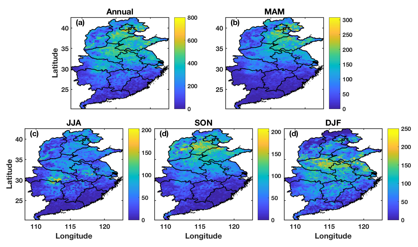
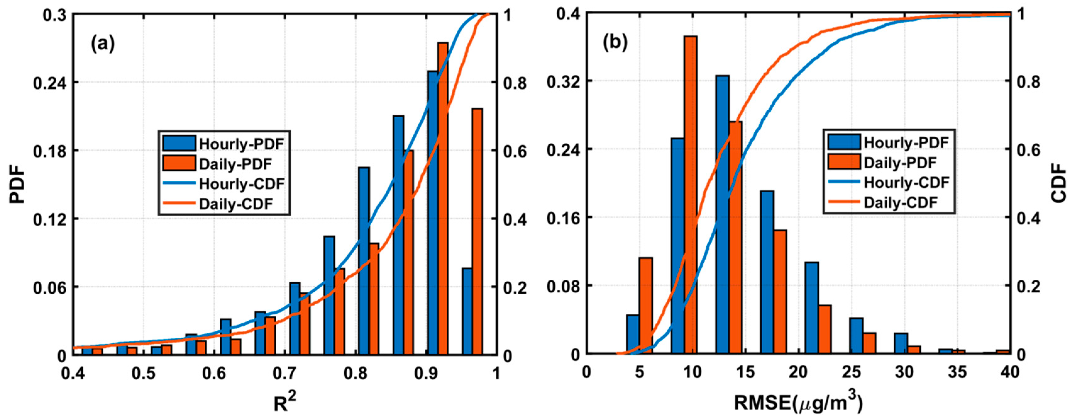
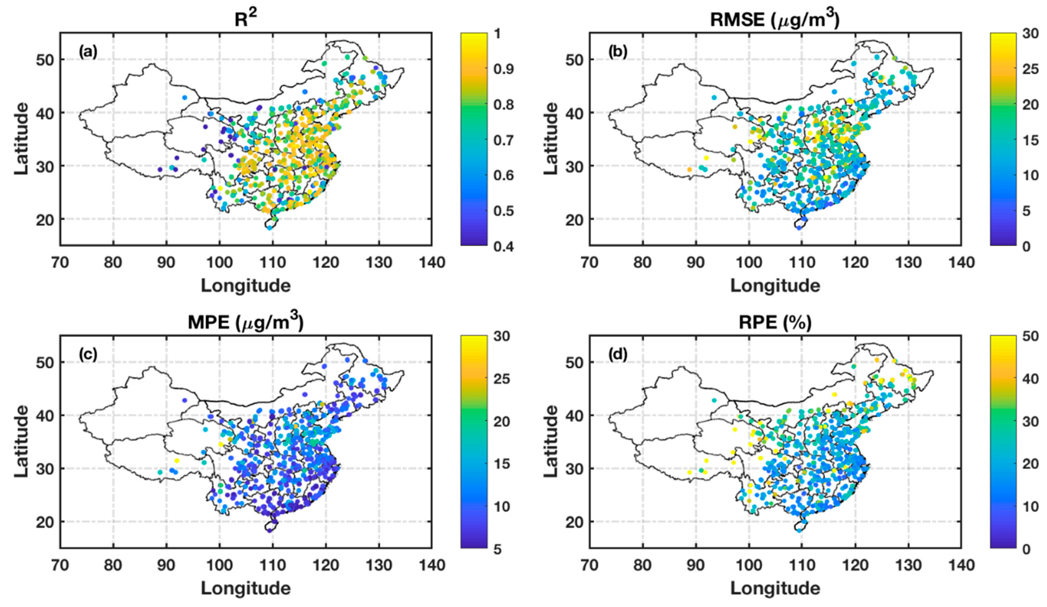
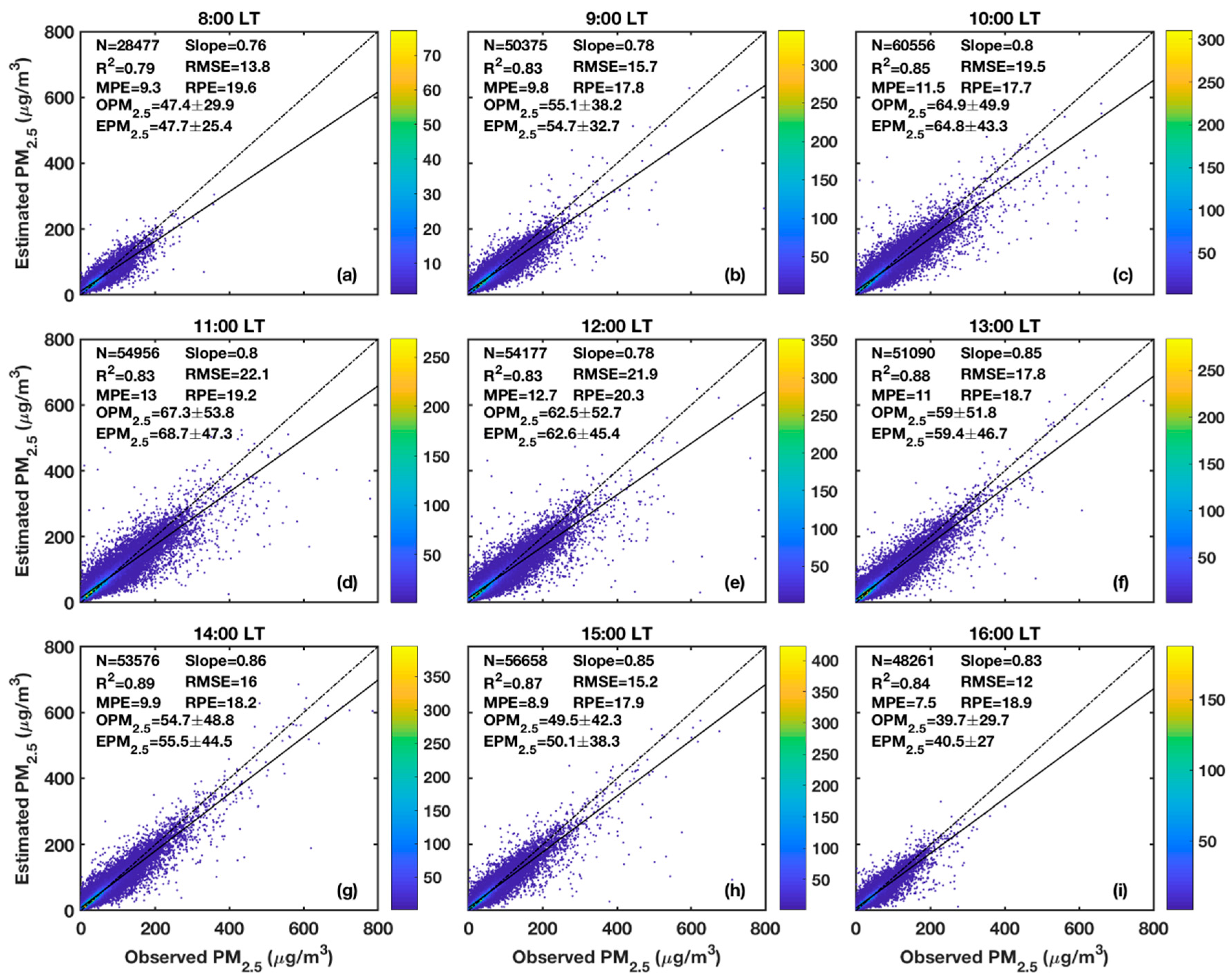
3.1. Descriptive Statistics

Figure 1 shows the probability distribution functions (PDFs) and cumulative distribution functions (CDFs) along with descriptive statistics of the modeling variables in the training dataset. The AOD has a mean and standard deviation of 0.32 and 0.24, respectively, with 80% of the values less than 0.5. The corresponding hourly ground-level PM2.5 concentrations range from 1 μg m−3 to ~1000 μg m−3 with a mean and standard deviation of 55 and 46 μg m−3, respectively. More than 90% of PM2.5 concentrations are less than 100 μg m−3. AODs and PM2.5 concentrations have a similar frequency distribution at the lower bounds of their value ranges. The meteorological variables are more variable and have nearly normal distributions. The distribution of PBLHs shows that a large number of samples are associated with low PBLHs. This is possible because the PBLH is only available at 00:00 and 12:00 UTC, corresponding to 08:00 and 20:00 local time (LT). Compared with the PBLH at noon, the PBLH is lower in the early morning and late afternoon.

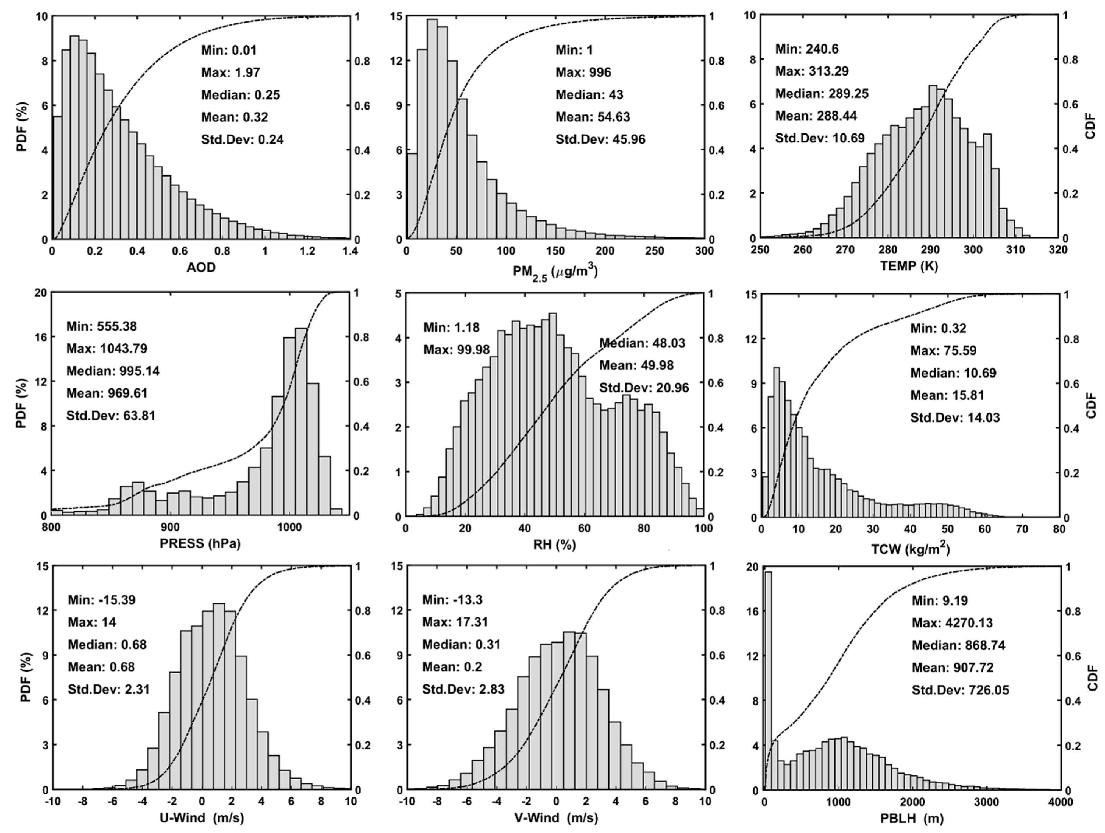
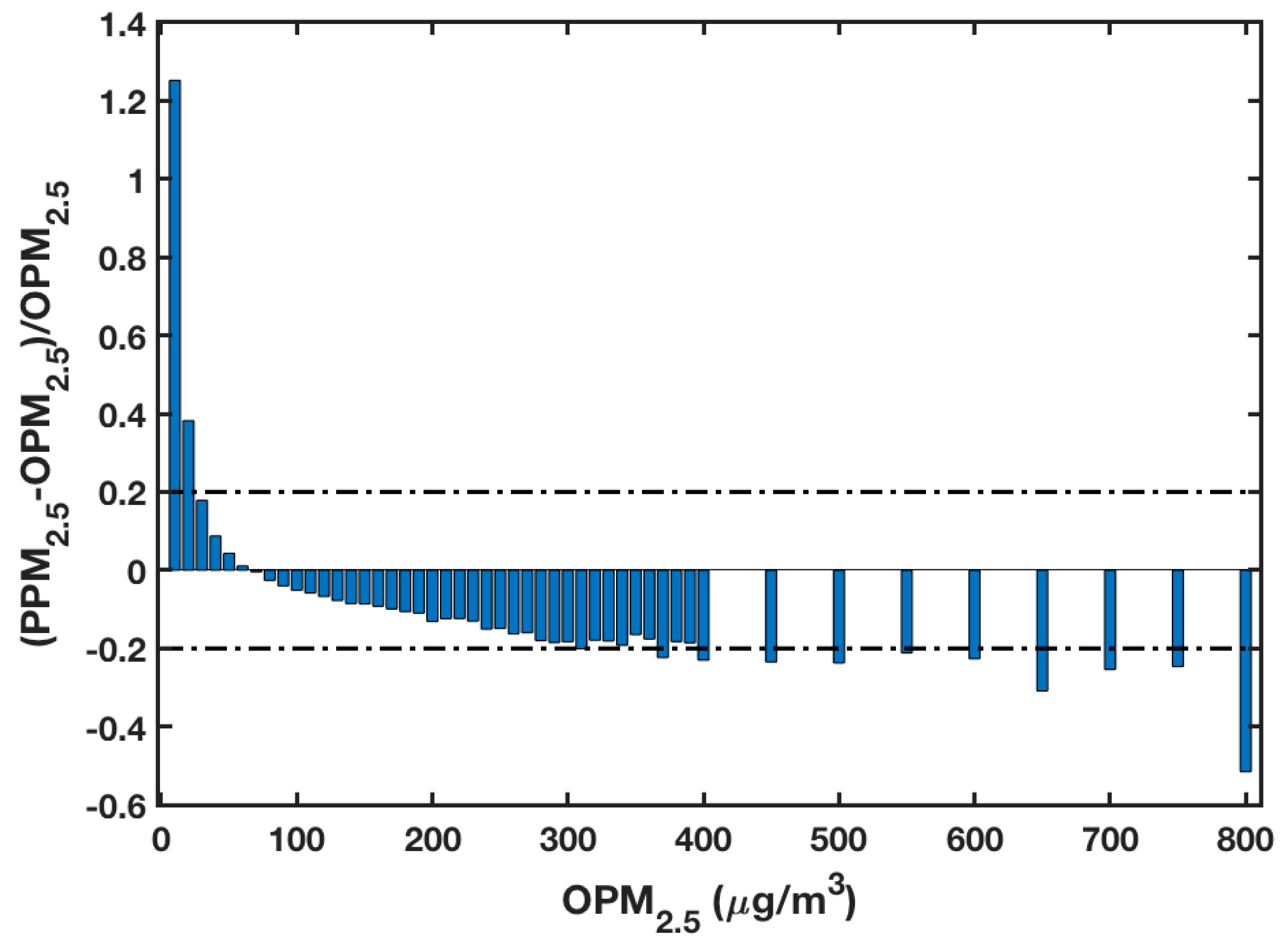
3.2. Model Fitting and Validation

Figure 2 shows scatter plots displaying the model fitting and 10-fold CV results of the RF model. The R2 for the model fitting is 0.86, and the RMSE and MPE are 17 and 10 μg m−3, respectively. The model CV has the same R2, and RMSE and MPE are increased by 0.3 to 17.3 μg m−3 and 10.3 μg m−3, respectively. This suggests that there is no substantial model overfitting. Figure 3 shows the PDFs and CDFs of CV R2 and RMSE for hourly and daily PM2.5 concentrations. R2 ranges from 0.28 to 0.97, with more values located between 0.8 and 0.95. Approximately 70% of the R2 values are greater than 0.8. The PDFs and CDFs of RMSE for hourly PM2.5 concentrations show that the local RMSE varies from 4 to 40 μg m−3 with most of the values located between 5 and 20 μg m−3 (Figure 3b). More than 80% of the values are less than 20 μg m−3. The biases of model CV-estimated PM2.5 concentrations are also defined and calculated as the difference between model-estimated and observed PM2.5 concentrations. About 87% and 70% of the biases fall in the range of −20 to 20 μg m−3 and −10 to 10 μg m−3, respectively, with a mean value of 0.4 μg m−3 (Figure S3). Many potential factors influence the relationship between PM2.5 and AOD and thus the model performance, including the number of samples, aerosol chemical composition, aerosol particle size, and weather conditions [42]. The aerosol composition influences the aerosol swelling, which increases the AOD but does not influence the PM2.5 concentration. The aerosol particle size determines the contribution of fine particles to the AOD. The following paragraph provides more discussion about this. Despite the poor model performance at some sites, the overall model performance is relatively high.
The seasonal and spatial variabilities of the model performance are also evaluated (Table 1 and Figure 4). The CV model has the highest R2 during the December–January–February (DJF) period (0.87), followed by the September–October–November (SON; 0.86), March–April–May (MAM; 0.82), and June–July–August (JJA; 0.72) periods. The RMSE and MPE are the largest and smallest during the DJF and JJA periods, respectively. These metrics provide different information about the model estimates. R2 represents how well the estimated and observed PM2.5 concentrations are correlated, and RMSE, MPE, and RPE demonstrate how close the absolute levels of these two PM2.5 concentrations are. The highest R2 during the DJF period was possibly due to the frequently observed stagnant atmosphere and low PBLH [43]. Under such conditions, more aerosols are constrained to the boundary layer, resulting in high surface PM2.5 concentrations and contributing to a large fraction of the boundary-layer AOD [44], which possibly increases the correlation between PM2.5 concentration and AOD. The low R2 during the JJA period likely occurred because of lower surface aerosol concentrations due to the higher PBLH, even though the AOD is large. Aerosol swelling due to the higher RH in the summertime partly explains this [44]. The large RMSE and MPE for the DJF period are partially attributed to the large variations in the surface PM2.5 concentration and the model-underestimated PM2.5 concentration under highly polluted conditions [15,45]. This will be discussed later. The spatial distribution of local R2 shown in Figure 4a indicates that higher R2 are found over areas with more densely distributed monitoring stations (e.g., East China), consistent with previous studies (e.g., [17]). Figure 4b,c show that the CV RMSE and MPE over the North China Plain, which has relatively high PM2.5 concentrations [5,17], are higher than over the other regions. Figure 4d shows that most of the CV RPEs are less than 20% with smaller values found over East China, a region with more densely distributed monitoring stations.
Figure 5 shows scatter plots of the comparison between model-estimated and surface-measured PM2.5 concentrations at different hours of the day. The CV R2 ranges from 0.79 to 0.89 with relatively high values between 1300 and 1500 LT and low values in the early morning. As previously discussed, many factors influence the model performance, including the number of samples, aerosol chemical composition, aerosol particle size, and weather conditions [42]. The larger solar zenith angle in the early morning may reduce the accuracy of Himawari-8 aerosol retrievals, which possibly weakens the model performance. The CV RMSEs (MPEs) vary between 10 and 22.1 μg m−3 (6.5 and 13 μg m−3). The CV RMSE and MPE at 1600 LT are smaller than at other hours, which may be due to the relatively small number of matchups. The CV RPE varies slightly with values between 17.7% and 20.3%. The high CV R2, low CV RMSE (MPE, RPE), and highly consistent values between observed and estimated PM2.5 concentrations at different hours suggest that the model can provide information about the diurnal cycle of PM2.5 concentrations, which will help improve the understanding of the evolution of PM2.5.
The CV of model-estimated PM2.5 concentrations versus surface-measured PM2.5 concentrations at daily, monthly, seasonal, and annual levels are also evaluated (Figure S4). Daily, monthly, seasonal, and annual PM2.5 contributions are derived from hourly PM2.5 concentrations by averaging over the respective periods. The CV R2 at the daily level is 0.92 and ranges from 0.30 to 0.99, with most values located between 0.85 and 1.0. Nearly 80% of the values are greater than 0.8 (Figure 3a). The PDF and CDF of RMSE at the daily level show that RMSE ranges from 2.8 to 40 μg m−3, with most values falling in the range of 5 to 15 μg m−3 (Figure 3b). The overall CV RMSE (MPE) and RPE at the daily level are 12.3 (7.7) μg m−3 and 13.7%, respectively. The biases of the model-estimated PM2.5 concentrations show that ~93% and 76% of the bias values fall in the range of −20 to 20 μg m−3 and −10 to 10 μg m−3, respectively (Figure S3b). Figure S4b–d shows that the CV R2 are 0.89, 0.9, and 0.9 at monthly, seasonal, and annual levels, respectively. The model-estimated seasonal mean PM2.5 concentration at each site is consistent with the seasonal mean surface measurement at that site. Seasonal mean biases agree well in all seasons at most sites (Figure S5). This suggests that compared to statistical measures based on hourly data, the model shows a better performance for PM2.5 estimates at daily, monthly, seasonal, and annual levels. Overall, the RF model predicts PM2.5 concentrations at different temporal scales well. The model can generate reasonable PM2.5 concentration estimates in areas where AODs are available. However, ground-level PM2.5 measurements are available at only a limited number of stations that are not uniformly distributed with more stations located in more densely populated regions. The spatial and temporal variations in PM2.5 concentration, especially at the hourly level, can now be provided in greater detail.
The overall CV slope (y-intercept) of model-estimated PM2.5 concentrations versus surface-measured PM2.5 concentrations is 0.82 (10.0) (Figure 2a), the CV slope (y-intercept) ranges from 0.76 (7.5) to 0.86 (14.6) at different hours of the day (Figure 5), and the CV slopes (y-intercepts) change from 0.82 (7.3) to 0.88 (9.7) at daily, monthly, seasonal, and annual levels (Figure S4). The result suggests that the model under- and over-estimates PM2.5 concentrations when PM2.5 concentrations are higher and lower than ~56 μg m−3, respectively. Figure 6 shows the variation in relative prediction error, i.e., [(estimated PM2.5 concentrations − observed PM2.5 concentrations)/observed PM2.5 concentrations], as a function of surface-observed PM2.5 concentrations. The model overestimates (underestimates) PM2.5 concentrations by more than 20% for PM2.5 concentrations less (greater) than 20 (400) μg m−3. Based on different algorithms, others have shown that their models underestimate (overestimate) PM2.5 concentrations (slopes of 0.73–0.88) when ground-level PM2.5 concentrations are higher (lower) than 60 μg m−3 [5,6,11,17,23,45,46,47,48]. This underestimation possibly happens for many reasons, e.g., the hygroscopicity of urban aerosols and the possibility of mixed types and layers of aerosols in the atmosphere [17]. Another possible reason is that the model training uses point-based PM2.5 measurements, which may not fully represent the spatial conditions of the collocated AOD pixel with a 5-km resolution. Also, aerosol retrievals based on the dark-target algorithm are not valid for heavy haze pollution because current cloud mask algorithms tend to mistake haze for clouds [49] and over bright surfaces in winter when high PM2.5 concentrations usually occur. Large variations in PM2.5 concentration may be overlooked if there are gaps in the satellite-retrieved AOD time series, which may contribute to the underestimation of PM2.5 concentrations under high pollution conditions [45]. This underestimation is likely a systematic error related to the complicated aerosol situation in China and the modeling framework [17].

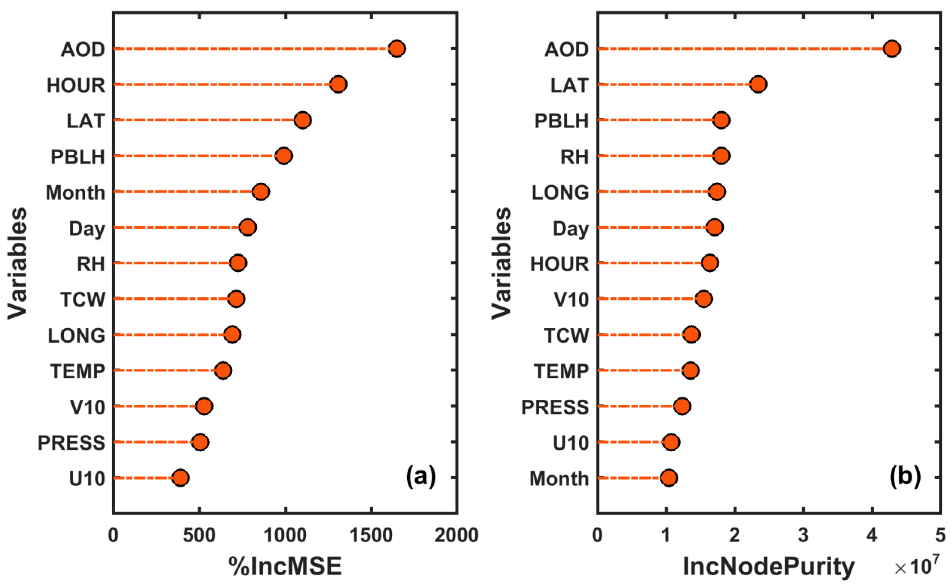
3.3. Variable Importance Assessment

Figure 7 illustrates the variable importance assessment for predictor variables in the model. The RF gives two measures of variable importance, namely, the increase in mean square error (%IncMSE) and the increase in node purities (IncNodePurity). The %IncMSE indicates the increase in the mean square error of the prediction if that variable is not involved in the training data. Thus, the higher the %IncMSE for a variable, the more important is that variable. The IncNodePurity represents the total mean increase in node purity from splitting on a predictor in the trees’ construction process. The larger the IncNodePurity of a predictor, the more important is that predictor [33,34]. AOD, PBLH, and regional variables (e.g., latitude) are among the top five most important predictor variables according to both importance measures. The AOD is related to the columnar aerosol concentration, and the PBLH significantly influences aerosol vertical and surface aerosol concentrations. These results also support our discussions on the model performance in different seasons (Section 3.2). The accuracies of both AOD and PBLH may thus play an important role in the model performance. The Discussion section elaborates on this. Note that estimating the variable importance in the RF algorithm is difficult, in general, because the importance of a variable may vary according to different combinations of input variables and numbers of samples in the training dataset.

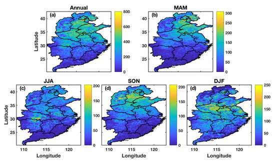
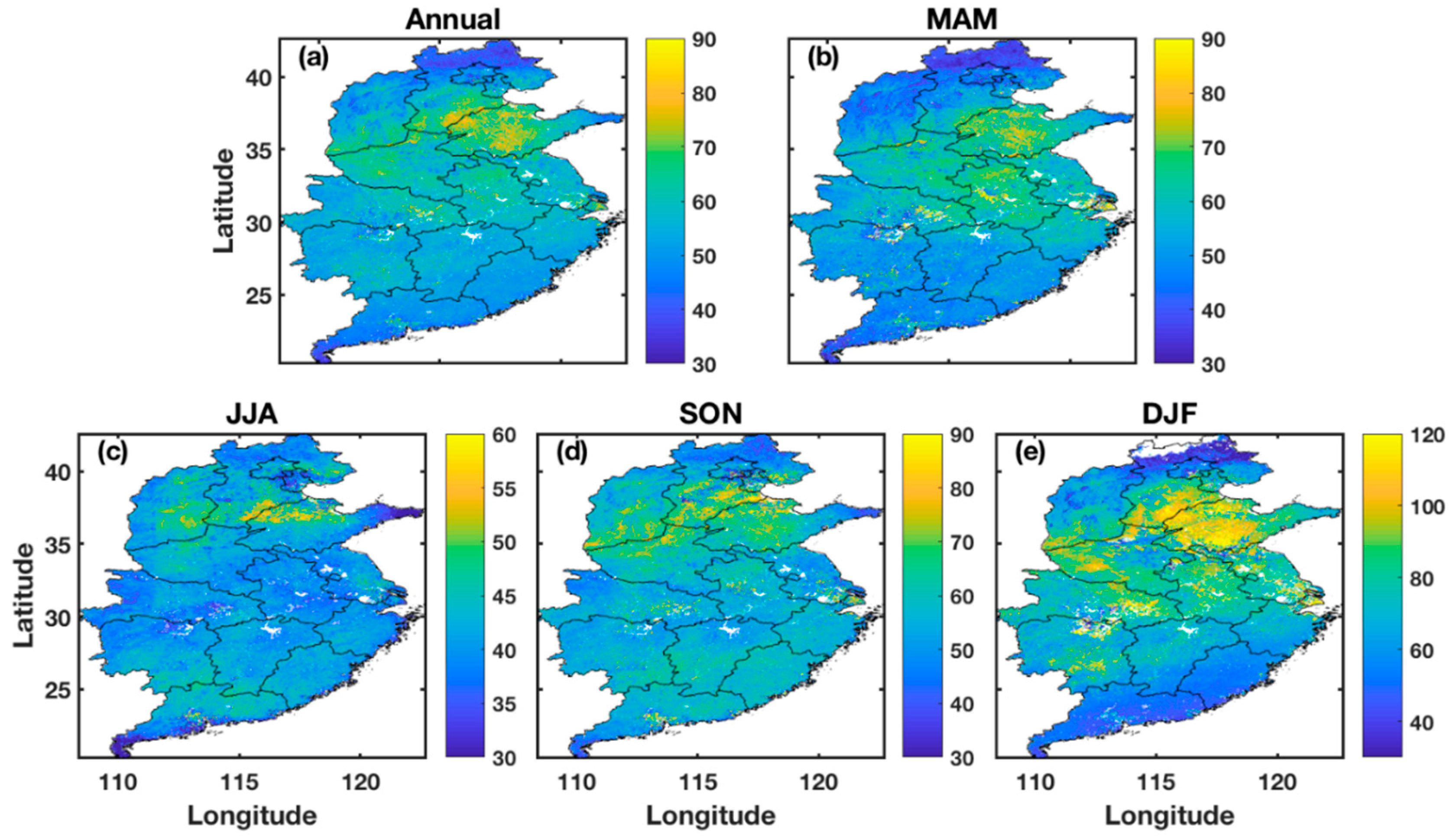
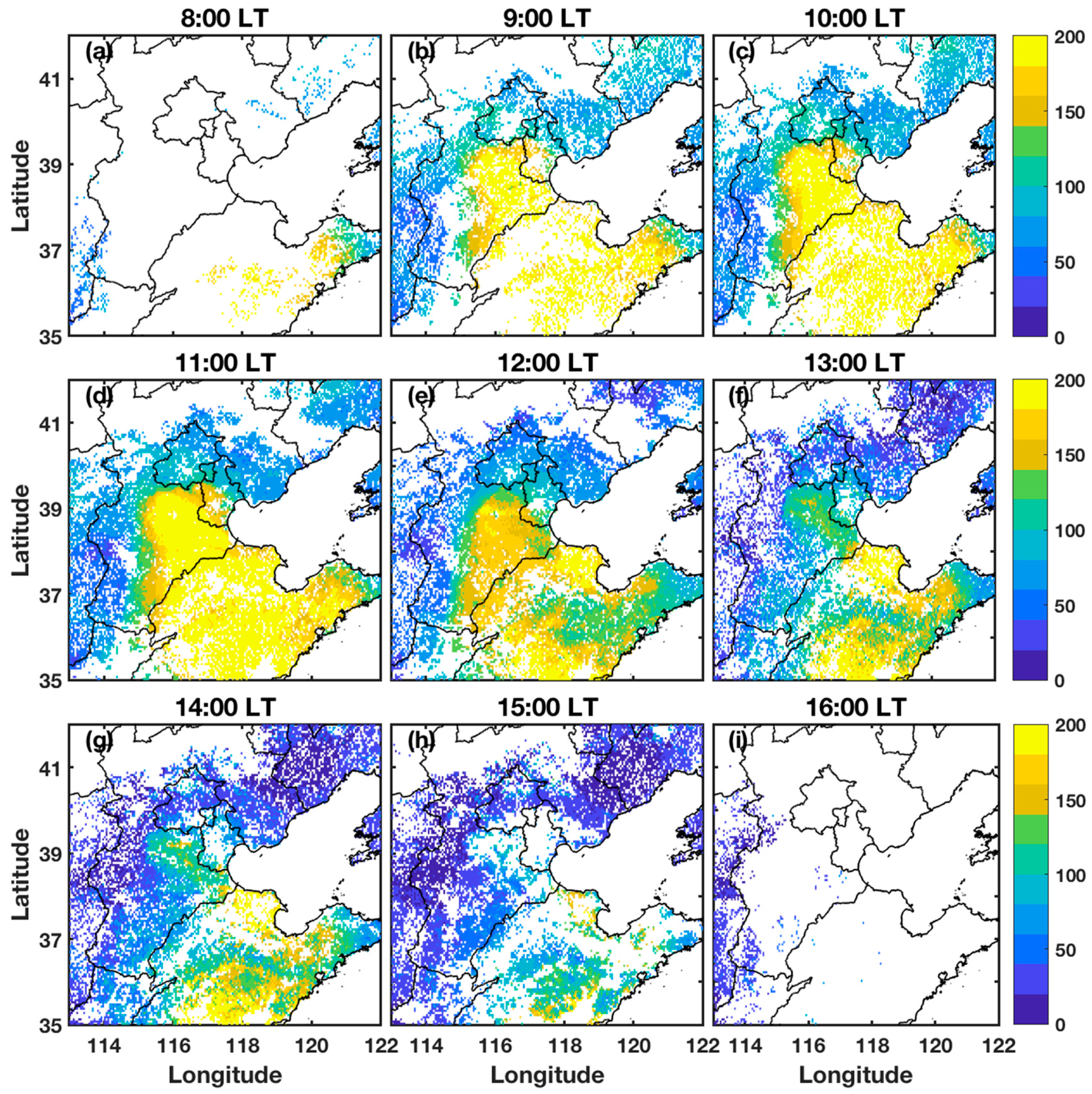
3.4. Spatiotemporal Distribution of Model-Estimated PM2.5 Concentrations over Central East China

Figure 8 shows the annual and seasonal mean distributions of PM2.5 concentration estimated by averaging the hourly model results over the central East China region where air pollution is relatively high. Figure S6 shows the corresponding annual and seasonal mean surface-observed PM2.5 concentrations. The spatiotemporal distributions of model-estimated and surface-observed PM2.5 concentrations are consistent. A north-to-south decreasing gradient is seen, which agrees with findings from previous studies (e.g., [5,17]). The heaviest pollution occurred in the southern parts of Hebei and Shanxi provinces, the northern part of Henan province, and the western part of Shandong province. The annual mean PM2.5 concentration over these regions was ~80–100 μg m−3. The dense concentration of local steel and power industries and rapid urbanization is responsible for this severe air pollution. PM2.5 concentrations over the middle part of central East Asia were slightly less than in the northern part with annual mean values falling in the range of 60 to 80 μg m−3. Compared with PM2.5 concentrations over the northern and middle parts of central East Asia, PM2.5 concentrations are generally lower than 60 μg m−3 in the south. Other than differences in the source of aerosols, the stagnant weather, weak winds, relatively low boundary layer heights, and lesser amount of precipitation over the northern region play important roles in the high PM2.5 concentrations there. The spatial distributions of PM2.5 concentrations in MAM and DJF are similar to the annual PM2.5 distributions, but the spatial distributions in JJA and SON are slightly different with the largest values in the northern region, followed by the southern region, and the lowest values in the middle part of central East Asia.
The seasonal spatial distributions of PM2.5 (Figure 8b–e) show that seasonal mean PM2.5 concentrations are the highest in winter, followed by fall and spring, and the lowest in summer. This could be related to the variation in local emissions and general atmospheric circulation conditions. Winter indoor heating in the northern region and stationary regional meteorological conditions contribute to high PM2.5 concentrations. With lower mixing layer heights and less precipitation, it is easy for pollutants to accumulate in the air. The lowest PM2.5 concentrations in the summertime occurred mainly because of prevailing unstable atmospheric conditions and heavier precipitation, which enhanced the dispersion, dilution, and diffusion of atmospheric pollutants. This reduces PM2.5 concentrations near the surface. The variation in seasonal mean PM2.5 concentration shown in this study is consistent with previous studies (e.g., [15,17]).
Figure 9 shows the spatial distributions of annual mean model-estimated PM2.5 concentrations over central East China for different hours of the day. Figure S7 shows the corresponding surface-observed PM2.5 concentrations. The model-estimated PM2.5 concentrations are generally consistent with surface-observed PM2.5 concentrations at each hour. The lowest mean PM2.5 concentrations occurred in the afternoon (1600 LT), and the highest mean PM2.5 concentration occurred before noon (1000 LT), consistent with results from studies focused on the Beijing–Tianjin–Hebei region [47]. Meteorological factors, among others, may have influenced this variation, which could synergistically affect PM2.5 concentrations [47]. For example, air pollution is dispersed more effectively in the afternoon than in the morning because the PBL is more stable and shallower in the morning than in the afternoon. However, this does not mean that PM2.5 concentrations always have the same diurnal cycle as the PBL since the relationship between PM2.5 concentrations and the PBL varies considerably with location, season, and other meteorological conditions [50]. Figure 9 also shows that during all hours of the day, PM2.5 concentrations are higher over the northern region and lower over the southern region, consistent with the spatial distribution of the annual mean PM2.5 concentration (Figure 8a).
Understanding of the general evolution of a high pollution episode is critical for epidemiological studies and pollution-controlling measures. Figure 10 shows the spatial distributions of model-estimated hourly PM2.5 concentrations for a high pollution episode that occurred on 14 January 2016 over the North China Plain. Figure S8 shows the corresponding surface-observed hourly PM2.5 concentrations. The PM2.5 concentrations from our model estimation are consistent with the PM2.5 concentrations from surface measurements at each hour. Northeast Hebei and Shandong provinces have the highest PM2.5 concentrations, with values greater than 200 μg m−3. PM2.5 concentrations are significantly higher in the morning than in the afternoon, consistent with the annual mean diurnal cycle of PM2.5 concentration (Figure 9). Figure S9 shows the mean diurnal cycle of model-estimated and surface-observed PM2.5 concentrations for six heavy PM2.5 episodes that occurred in winter over the North China Plain (35–42°N, ll3–122°E). The diurnal cycle of model-estimated PM2.5 concentrations is highly consistent with the diurnal cycle of surface-observed PM2.5 concentrations for all heavy pollution episodes examined. Our model appears to successfully capture the annual mean diurnal cycle of PM2.5 concentrations and the diurnal cycle of PM2.5 concentrations for a specific air pollution episode.

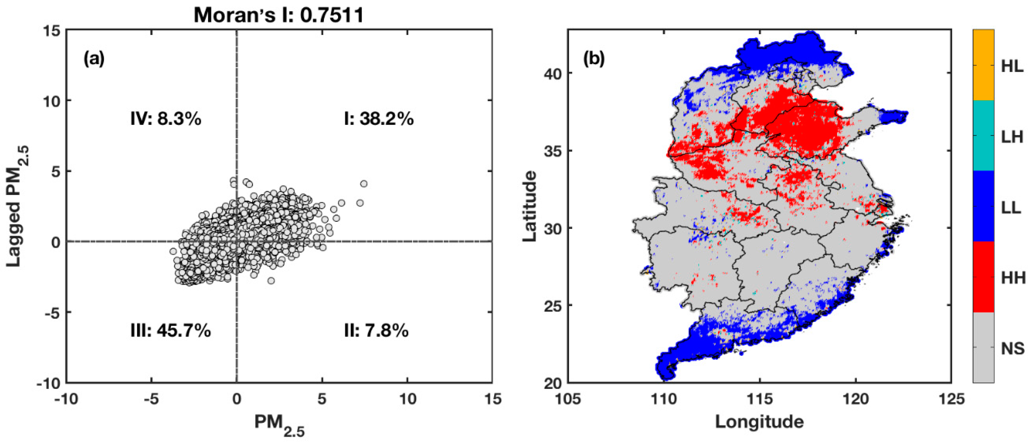
3.5. Spatial Agglomeration Pattern of Model-Estimated PM2.5 Concentrations over Central East China

Figure 11a,b show the scatter plot of the global MI and the spatial agglomeration diagram of annual PM2.5 concentrations over central East China, respectively. Figure S10 shows the same kind of plots for each season. Each spatial agglomeration diagram passes the significance test at a significance level (p) of 0.05. The scatter plot of MI shows four categories of spatial agglomeration pattern. The first (I) and third (III) categories represent the high-high (HH) and low-low (LL) aggregation patterns, meaning that the PM2.5 concentrations in a satellite pixel and in its surrounding pixels are both high and both low, respectively. The second (II) and fourth (IV) categories represent the high-low (HL) and low-high (LH) aggregation patterns, meaning that high (low) PM2.5 concentrations in areas are surrounded by low (high) PM2.5 concentrations. The PM2.5 concentrations over areas with HH (LL) and HL (LH) aggregation patterns are homogeneous and heterogeneous, respectively. The large positive global MI values indicate that, overall, PM2.5 concentrations have a significant (p < 0.05) positive spatial autocorrelation in central East China in each season and throughout the whole year. The global MI is highest in winter (DJF), indicating that the spatial spillover effect is higher, and PM2.5 concentrations are more homogeneous than in other seasons. Most of the samples in each season are in categories I and III (left panels of Figure S10). Figure 11b shows that mainly the LL and HH spatial agglomeration types characterize central East China. HH spatial clusters are mainly observed in the southern parts of Shanxi and Hebei provinces, the western and northern parts of Henan province, the western part of Shandong province, and part of northern Anhui province where high PM2.5 concentrations are also observed. LL spatial clusters are primarily located in the northern part of Hebei province, the eastern coastal region of Shandong province, the eastern coastal regions of Zhejiang and Fujian provinces, and most of Guangdong province where PM2.5 concentrations are also relatively low. The seasonal distributions of the HH and LL spatial clusters (right panels of Figure S10) are consistent with the seasonal distributions of the high and low PM2.5 concentrations (Figure 8b–e). The short-term (daily) spatial distribution of PM2.5 concentrations and their relevant spatial agglomeration characteristics over central Eat China are also evaluated based on two different pollution cases (Figure S11). One case is a severe pollution episode that occurred on 2 January 2016 over the North China Plain, and the other case is a moderate pollution episode that occurred on 28 July 2016. Similar to the annual and seasonal distributions of spatial agglomeration, the daily spatial distribution of MI clustering is also highly consistent with the daily distribution of PM2.5 concentrations.

4. Discussion

4.1. Comparison with Previous Studies

It is well known that the relationship between AOD and PM2.5 concentration is affected by multiple factors (e.g., aerosol type, meteorological variables), making the relationship more complicated. Machine learning, a newly developed method of data analysis, may better capture this complex relationship over large spatial and temporal scales compared to traditional regression algorithms. This study estimated hourly PM2.5 concentrations based on the RF model, a type of ensemble learning algorithm, which is a nonparametric, nonlinear, and multivariate regression algorithm. Table S1 lists some previous studies on estimating PM2.5 concentrations from satellite remote sensing over China based on statistical models. R2 have ranged from 0.18 to 0.87 in regional-scale studies and from 0.24 to 0.88 in national-scale studies. Both depend on the different selected models and input predictor variables. In almost all of the studies, the primary predictor, AOD, was derived from MODIS retrievals with one or two observations per day, and daily mean PM2.5 concentrations were estimated from that. The CV of the RF model in our study shows that the model estimates PM2.5 concentrations well at the hourly level with an R2 of 0.86 and an RMSE of 17.3 μg m−3. The CV R2 and RMSE at the daily level are 0.92 and 12.3 μg m−3, respectively. The performance of our RF model is better than that of many models from previous similar studies and is comparable to some machine learning approaches (e.g., [17]; see Table S1). Compared with other machine learning approaches, the RF approach is based on a simple, one-stage structure and is user friendly. It can address the problem of complex interactions and highly correlated predictor variables [33]. Apart from the good performance and advantages of the approach we used, the model developed in the current study to estimate hourly mean PM2.5 concentrations can provide information about the diurnal cycle of PM2.5 concentration at a fine spatial resolution. This will improve our understanding of the evolution of PM2.5.

4.2. Potential Limitations and Room for Model Improvement

Although the model can predict PM2.5 concentrations well, there are still potential limitations and room for future algorithm improvements. The assessment of the relative importance of different variables in Section 3.3 shows that AOD and PBLH are the most important predictors for the model performance. Due to the lack of high spatial- and temporal-resolution observations of the PBLH, reanalysis data are commonly used in most studies and also in the current study. The PBLH product is only available twice daily, which may have some effect on estimating hourly PM2.5 concentrations with our model. Note that the PBLH is not completely independent from other meteorological variables such as the surface temperature. Since the other meteorological variables (e.g., surface temperature) are measured four times a day, the evolution of meteorological conditions can be monitored. If high-frequency meteorological data were available, the model performance would improve. Many techniques have been developed to determine the PBLH, for example, through radiosonde measurements, remote sensing, laboratory experiments, and model simulations [51]. PBLHs from these methods show significant differences for both the stable and convective boundary layer. Zang et al. [52] incorporated the PBLH into a regression model of AOD to PM2.5, noting that different methods derived optimal PBLHs for the stable boundary layer and convective layer. Su et al. [53] showed that using lidar observations to estimate PBLHs was effective for PM2.5 remote sensing. Improving the AOD-PM2.5 model by considering both stable and convective PBLHs and using measurements instead of reanalysis data may enhance the accuracy of estimated PM2.5 concentrations.
A geostationary satellite can overcome the problem of PM2.5 estimates from polar-orbiting satellite retrievals with a low frequency. Himawari-8 can provide AODs every 10 min. Since the accuracy evaluation of Himawari-8 aerosol products is limited, studies have shown that the accuracy of Himawari-8 AOD retrievals still needs to be improved compared with surface Aerosol Robotic Network and MODIS retrievals [47]. The AHI-retrieved AOD over Eastern China suffers from an obvious underestimation compared with ground-based and MODIS observations [54]. Figure S12 shows a comparison of AHI and MODIS AODs over all PM2.5 sites. MODIS Terra and Aqua 3-km AOD retrievals with the highest confidence levels from pixels falling within 5 km of each PM2.5 site were averaged and matched with the training dataset. AHI AODs are significantly and systematically lower than MODIS AODs with large RMSE and MPE, consistent with previous studies (e.g., [47,54]). PM2.5 concentrations are also estimated from AHI and MODIS AODs using the RF algorithm. Figure S13 shows scatter plots of the cross-validation results. Although AHI AODs are significantly lower than MODIS AODs, the performance of the RF model using AHI AODs is comparable with, even somewhat better than, that using MODIS AODs. This suggests that errors in AOD, especially the bias, do not necessarily affect the machine-learning-based retrievals of PM2.5, especially if the error is systematic. Like many previous studies, total columnar AODs are used to estimate ground-level PM2.5 concentrations in the current study. However, PM2.5 concentrations are likely more related to fine aerosol particles. Compared to the total AOD, the AOD for fine-mode particles is more correlated with ground-level PM2.5 concentrations [55,56,57]. The fine-mode fraction (FMF) can be used to separate the contributions from smaller and larger particles to the total AOD and to calculate the fine-mode AOD. However, current FMF retrievals from satellite still suffer from significant uncertainties, limiting the application of the fine-mode AOD in PM2.5 estimations from satellite remote sensing. A look-up-table-based spectral deconvolution algorithm for FMF retrievals was developed by Yan et al. [58] and incorporated into a model to estimate PM2.5 from MODIS retrievals. The accuracy of these PM2.5 estimates improved when the fine-mode AOD was used instead of the total AOD [57].
More predictor variables, e.g., land-use variables (forest cover and water cover), population data, and elevation data, were used in previous studies for model development (e.g., [5,59]). We did not include these data in our RF model, a limitation that will be examined in future work. It is possible that the model performance would improve if these data were considered. Even though we did not include more predictor variables, our model performed as well as, if not better, than those from similar studies.

5. Conclusions

Most studies have focused on making daily PM2.5 estimations using polar-orbiting satellite data (e.g., from the MODIS) which are inadequate for understanding the evolution of PM2.5. The current study developed a multivariable model by incorporating Himawari-8 AODs and meteorological parameters to estimate surface PM2.5 concentrations at an hourly scale based on an ensemble learning algorithm. The model performance was evaluated using the 10-fold across-validation technique and several statistical indicators, including R2, RMSE, MPE, and RPE between CV-estimated and observed PM2.5 concentrations. The CV results showed that the model predicts PM2.5 concentrations well at the hourly level with R2 and RMSE values of 0.86 and 17.3 μg m−3, respectively. About 70% of the R2 values are greater than 0.8, and more than 80% of the RMSE values are less than 20 μg m−3. Model results are better in fall and winter, and over regions with more densely distributed monitoring stations. The model also estimates PM2.5 concentrations well at daily, monthly, seasonal, and annual levels.
The spatial distribution of annual mean PM2.5 concentrations in central East China derived from our model shows a north-to-south decreasing gradient with high concentrations in the northern part of the region and low concentrations in the southern part. Seasonal spatial distributions of PM2.5 concentration show that seasonal mean PM2.5 concentrations are the highest in winter, followed by fall and spring, and the lowest in summer. Estimated PM2.5 concentrations are lowest in the early morning and late afternoon. PM2.5 concentrations exhibit a significant (p < 0.05) spatial agglomeration effect in central East China for each season and throughout the whole year.
The AHI AODs are significantly lower than MODIS AODs, but the performance of the RF model using AHI AODs is comparable with, even somewhat better than, that using MODIS AODs. Errors in AOD do not necessarily affect the machine-learning-based retrieval accuracy of PM2.5 proportionally, especially if the error is systematic. The model presented in this study has the capacity to identify PM2.5 spatial distributions at various scales, especially at the hourly level. It can potentially improve our understanding of the diurnal cycle and general evolution of PM2.5, as well as the sources, the formation processes, transportation, and diffusion behavior of regional PM2.5 pollution episodes. This would also help develop sound pollution-controlling measures. The model products are also useful for studying the influence of air pollution on human health, a topic that has drawn increasing attention from public health, government, and scientific communities.

Supplementary Materials

The following are available online at https://0-www-mdpi-com.brum.beds.ac.uk/2072-4292/11/18/2120/s1. Figure S1. The number of (a) annual and (b–e) seasonal AHI Level-3 AODs with the highest confidence level over central East China from 1 January 2016 to 31 December 2016. The seasons are defined by groups of months: spring (March–April–May, or MAM), summer (June–July–August, or JJA), autumn (September–October–November, or SON), and winter (December–January–February, or DJF). Figure S2. Spatial distribution of PM2.5 monitoring sites in mainland China used in this study. Figure S3. Histograms of the biases of model cross-validation-estimated PM2.5 concentrations at (a) hourly and (b) daily levels. Each panel shows the percentage of samples falling within two ranges of values (in square brackets). Figure S4. Scatter plots of the cross-validation of estimated PM2.5 concentrations by comparing surface-measured PM2.5 concentrations at (a) daily, (b) monthly, (c) seasonal, and (d) annual levels. The dashed lines are 1:1 lines. N: number of samples; R2: coefficient of determination; RMSE: root-mean-square error (μg m−3); MPE: mean prediction error (μg m−3); RPE: relative prediction error (%). Figure S5. Differences between model-estimated and surface-measured seasonal mean PM2.5 concentrations at each site in different seasons: (a) March, April, and May (MAM), (b) June, July, and August (JJA), (c) September, October, and November (SON), and (d) December, January, and February (DJF). Units are μg m−3. Figure S6. Surface-observed PM2.5 concentrations (μg m−3) over central East China: (a) for the whole year of 2016, (b) March, April, and May (MAM), (c) June, July, and August (JJA), (d) September, October, and November (SON), and (e) December, January, and February (DJF). Figure S7. Spatial distributions of mean surface-measured PM2.5 concentrations (μg m−3) over central East China for (a-i) different hours of the day (0800–1600 local time, or LT). Figure S8. Spatial distributions of surface-measured hourly PM2.5 concentrations (μg m−3) for a high pollution episode that occurred on 14 January 2019 over the North China Plain for (a-i) different hours of the day (8:00-16:00 LT). LT: local time. Figure S9. Diurnal cycles of mean model-estimated (red bars) and surface-observed (blue bars) PM2.5 concentrations with standard deviations for (a-f) several high PM2.5 episodes that occurred over the North China Plain (35–42°N, 113–122°E; LT: local time). The dates are in the YYYYMMDD format where YYYY = year, MM = month, and DD = day. Figure S10. Left panels: Scatter plots of the global Moran Index for the four seasons (from top to bottom, March–April–May (MAM), June–July–August (JJA), September–October–November (SON), and December–January–February (DFJ). Right panels: Spatial agglomeration diagrams of seasonal model-estimated PM2.5 concentrations over central East China for the four seasons. The numbers in the left panels are the percentages of samples with the aggregation patterns of (going clockwise from the upper right) I, II, III, and IV. The spatial agglomeration diagrams pass the significance test at a significance level of 0.05. The legends on the right give the spatial agglomeration category: high-low (HL), low-high (LH), low-low (LL), high-high (HH), and no significance (NS). Figure S11. Spatial distributions of PM2.5 concentrations (a,c) and their relevant spatial agglomeration characteristics (b,d) for a high pollution episode that occurred on 2 January 2016 over the North China Plain (a,b) and a relatively low pollution episode that occurred on 28 July 2016 (c,d). The spatial agglomeration diagrams pass the significance test at a significance level of 0.05. The legends in (b,d) give the spatial agglomeration category: high-low (HL), low-high (LH), low-low (LL), high-high (HH), and no significance (NS). Figure S12. Scatter plot of the AHI-retrieved AOD as a function of MODIS-retrieved AOD at 500 nm over all PM2.5 sites in 2016. The dashed line is the 1:1 line. N: number of samples; R2: coefficient of determination; RMSE: root-mean-square error (μg m−3). Figure S13. Scatter plots of cross-validation of the RF model of (a) AHI AOD and (b) MODIS AOD. The dashed lines are 1:1 lines. N: number of samples; R2: coefficient of determination; RMSE: root-mean-square error (μg m−3); MPE: mean prediction error (μg m−3); RPE: relative prediction error. Table S1. Summary of estimates of PM2.5 concentrations from satellite AODs based on statistical models at regional and national scales in China. NA stands for “not available”.

Author Contributions

Conceptualization, J.L. and F.W.; data curation, J.L.; investigation, J.L. and Z.L.; methodology, J.L.; validation, J.L.; writing—original draft, J.L.; writing—review and editing, J.L., F.W., Z.L., and M.C.C.

Funding

This research was funded by the National Key Research and Development Program of China “Development of Meteorological Satellite Remote Sensing Technology and Platform for Global Monitoring, Assessments and Applications” under the funding code of 2018YFC1506500 and National Key Research and Development Program of China (2017YFC1501702).

Acknowledgments

ERA-Interim reanalysis data were downloaded from http://apps.ecmwf.int/datasets/data/interim-full-daily/levtype=sfc/. The Japan Meteorological Agency’s JAXA P-Tree system provides the Himawari Standard Data.

Conflicts of Interest

The authors declare no conflict of interest.

References

  1. Burnett, R.T.; Pope, C.A., III; Ezzati, M.; Olives, C.; Lim, S.S.; Mehta, S.; Shin, H.H.; Singh, G.; Hubbell, B.; Brauer, M.; et al. An integrated risk function for estimating the global burden of disease attributable to ambient fine particulate matter exposure. Environ. Health Perspect. 2014, 122, 397–403. [Google Scholar] [CrossRef] [PubMed]
  2. Apte, J.S.; Marshall, J.D.; Cohen, A.J.; Brauer, M. Addressing global mortality from ambient PM2.5. Environ. Sci. Technol. 2015, 49, 8057–8066. [Google Scholar] [CrossRef] [PubMed]
  3. Kan, H.D.; Chen, B.H. Meta-analysis of exposure–response functions of air particulate matter and adverse health outcomes in China. J. Environ. Health 2002, 19, 422–424. [Google Scholar]
  4. Lelieveld, J.; Evans, J.; Fnais, M.; Giannadaki, D.; Pozzer, A. The contribution of out-door air pollution sources to premature mortality on a global scale. Nature 2015, 525, 367–371. [Google Scholar] [CrossRef] [PubMed]
  5. Ma, Z.; Hu, X.; Sayer, A.M.; Levy, R.; Zhang, Q.; Xue, Y.; Tong, S.; Bi, J.; Huang, L.; Liu, Y. Satellite-based spatiotemporal trends in PM2.5 concentrations: China, 2004–2013. Environ. Health Perspect. 2016, 124, 184–192. [Google Scholar] [CrossRef] [PubMed]
  6. Yu, W.; Liu, Y.; Ma, Z.; Bi, J. Improving satellite-based PM2.5 estimates in China using Gaussian processes modeling in a Bayesian hierarchical setting. Sci. Rep. 2017, 7, 7048. [Google Scholar] [CrossRef] [PubMed]
  7. Liu, Y.; Park, R.J.; Jacob, D.J.; Li, Q.; Kilaru, V.; Sarnat, J.A. Mapping annual mean ground-level PM2.5 concentrations using Multiangle Imaging Spectroradiometer aerosol optical thickness over the contiguous United States. J. Geophys. Res. 2004, 109, D22206. [Google Scholar] [CrossRef]
  8. Geng, G.; Zhang, Q.; Martin, R.V.; van Donkelaar, A.; Huo, H.; Che, H.; Lin, J.; He, K. Estimating long-term PM2.5 concentrations in China using satellite-based aerosol optical depth and a chemical transport model. Remote Sens. Environ. 2015, 166, 262–270. [Google Scholar] [CrossRef]
  9. Van Donkelaar, A.; Martin, R.V.; Brauer, M.; Kahn, R.; Levy, R.; Verduzco, C.; Villeneuve, P.J. Global estimates of ambient fine particulate matter concentrations from satellite-based aerosol optical depth: Development and application. Environ. Health Perspect. 2010, 118, 847–855. [Google Scholar] [CrossRef]
  10. Van Donkelaar, A.; Martin, R.V.; Spurr, R.J.D.; Drury, E.; Remer, L.A.; Levy, R.C.; Wang, J. Optimal estimation for global ground-level fine particulate matter concentrations. J. Geophys. Res. Atmos. 2013, 118, 5621–5636. [Google Scholar] [CrossRef] [Green Version]
  11. Lin, C.; Li, Y.; Yuan, Z.; Lau, A.K.H.; Li, C.; Fung, J.C.H. Using satellite remote sensing data to estimate the high-resolution distribution of ground-level PM2.5. Remote Sens. Environ. 2015, 156, 117–128. [Google Scholar] [CrossRef]
  12. Zhang, Y.; Li, Z. Remote sensing of atmospheric fine particulate matter (PM2.5) mass concentration near the ground from satellite observation. Remote Sens. Environ. 2015, 160, 252–262. [Google Scholar] [CrossRef]
  13. Engel-Cox, J.A.; Holloman, C.H.; Coutant, B.W.; Hoff, R.M. Qualitative and quantitative evaluation of MODIS satellite sensor data for regional and urban scale air quality. Atmos. Environ. 2004, 38, 2495–2509. [Google Scholar] [CrossRef]
  14. Lee, H.J.; Liu, Y.; Coull, B.A.; Schwartz, J.; Koutrakis, P. A novel calibration approach of MODIS AOD data to predict PM2.5 concentrations. Atmos. Chem. Phys. 2011, 11, 7991–8002. [Google Scholar] [CrossRef]
  15. Ma, Z.W.; Hu, X.F.; Huang, L.; Bi, J.; Liu, Y. Estimating ground-level PM2.5 in China using satellite remote sensing. Environ. Sci. Technol. 2014, 48, 7436–7444. [Google Scholar] [CrossRef] [PubMed]
  16. Liu, Y. Monitoring PM2.5 from space for health: Past, present, and future directions. Environ. Manag. 2014, 6, 6–10. [Google Scholar]
  17. Li, T.; Shen, H.; Yuan, Q.; Zhang, X.; Zhang, L. Estimating ground level PM2.5 by fusing satellite and station observations: A geo-intelligent deep learning approach. Geophys. Res. Lett. 2017, 44, 11985–11993. [Google Scholar] [CrossRef]
  18. Wang, W.; Primbs, T.; Tao, S.; Simonich, S.L.M. Atmospheric particulate matter pollution during the 2008 Beijing Olympics. Environ. Sci. Technol. 2009, 43, 5314–5320. [Google Scholar] [CrossRef]
  19. Gupta, P.; Christopher, S.A. Particulate matter air quality assessment using integrated surface, satellite, and meteorological products: Multiple regression approach. J. Geophys. Res. 2009, 114, D14205. [Google Scholar] [CrossRef]
  20. Zhang, H.; Hoff, R.M.; Engel-Cox, J.A. The relation between Moderate Resolution Imaging Spectroradiometer (MODIS) aerosol optical depth and PM2.5 over the United States: A geographical comparison by U.S. Environmental Protection Agency regions. J. Air Waste Manag. 2009, 59, 1358–1369. [Google Scholar] [CrossRef]
  21. Hu, X.; Waller, L.A.; Al-Hamdan, M.Z.; Crosson, W.L.; Ester, M.G.; Estes, S.M.; Quattrochi, D.A.; Sarnat, J.A.; Liu, Y. Estimating ground-level PM2.5 concentrations in the southeastern US using geographically weighted regression. Environ. Res. 2013, 121, 1–10. [Google Scholar] [CrossRef]
  22. Song, W.; Jia, H.; Huang, J.; Zhang, Y. A satellite-based geographically weighted regression model for regional PM2.5 estimation over the Pearl River Delta region in China. Remote Sens. Environ. 2014, 154, 7. [Google Scholar] [CrossRef]
  23. You, W.; Zang, Z.; Zhang, L.; Li, Y.; Wang, W. Estimating national-scale ground-level PM2.5 concentration in China using geographically weighted regression based on MODIS and MISR AOD. Environ. Sci. Pollut. Res. 2016, 23, 8327–8338. [Google Scholar] [CrossRef]
  24. Lee, H.J.; Coull, B.A.; Bell, M.L.; Koutrakis, P. Use of satellite-based aerosol optical depth and spatial clustering to predict ambient PM2.5 concentrations. Environ. Res. 2012, 118, 8–15. [Google Scholar] [CrossRef]
  25. Xie, Y.; Wang, Y.; Zhang, K.; Dong, W.; Lv, B.; Bai, Y. Daily estimation of ground-level PM2.5 concentrations over Beijing using 3-km resolution MODIS AOD. Environ. Sci. Technol. 2015, 49, 12280–12288. [Google Scholar] [CrossRef]
  26. Liu, Y.; Paciorek, C.J.; Koutrakis, P. Estimating regional spatial and temporal variability of PM2.5 concentrations using satellite data, meteorology, and land use information. Environ. Health Perspect. 2009, 117, 886–892. [Google Scholar] [CrossRef]
  27. Fang, X.; Zou, B.; Liu, X.; Sternberg, T.; Zhai, L. Satellite-based ground PM2.5 estimation using timely structure adaptive modeling. Remote Sens. Environ. 2016, 186, 152–163. [Google Scholar] [CrossRef]
  28. Lv, B.; Hu, Y.; Chang, H.H.; Russell, A.G.; Cai, J.; Xu, B.; Bai, Y. Daily estimation of ground-level PM2.5 concentrations at 4-km resolution over Beijing-Tianjin-Hebei by fusing MODIS AOD and ground observations. Sci. Total Environ. 2017, 580, 235–244. [Google Scholar] [CrossRef]
  29. Lv, B.; Hu, Y.; Chang, H.H.; Russell, A.G.; Bai, Y. Improving the accuracy of daily PM2.5 distributions derived from the fusion of ground-level measurements with aerosol optical depth observations, a case study in North China. Environ. Sci. Technol. 2016, 50, 4752–4759. [Google Scholar] [CrossRef]
  30. Breiman, L. Statistical modeling: The two cultures. Stat. Sci. 2001, 16, 199–215. [Google Scholar] [CrossRef]
  31. Zhan, Y.; Luo, Y.; Deng, X.; Chen, H.; Grieneisen, M.; Shen, X.; Zhu, L.; Zhang, M. Spatiotemporal prediction of continuous daily PM2.5 concentrations across China using a spatially explicit machine learning algorithm. Atmos. Environ. 2017, 155, 129–139. [Google Scholar] [CrossRef]
  32. Hou, W.; Li, Z.; Zhang, Y.; Xu, H.; Zhang, Y.; Li, K.; Li, D.; Wei, P.; Ma, Y. Using support vector regression to predict PM10 and PM2.5. IOP Conf. Ser. Earth Environ. Sci. 2014, 17, 012268. [Google Scholar]
  33. Hu, X.; Belle, J.H.; Meng, X.; Wildani, A.; Waller, L.A.; Strickland, M.J.; Liu, Y. Estimating PM2.5 concentrations in the conterminous United States using the random forest approach. Environ. Sci. Technol. 2017, 51, 6936–6944. [Google Scholar] [CrossRef]
  34. Liaw, A.; Wiener, M. Classification and regression by randomForest. R News 2002, 2, 18–22. [Google Scholar]
  35. Liu, Y.; Franklin, M.; Kahn, R.; Koutrakis, P. Using aerosol optical thickness to predict ground-level PM2.5 concentrations in the St. Louis area: A comparison between MISR and MODIS. Remote Sens. Environ. 2007, 107, 33–44. [Google Scholar] [CrossRef]
  36. Wu, J.; Yao, F.; Li, W.; Si, M. VIIRS-based remote sensing estimation of ground-level PM2.5 concentrations in Beijing−Tianjin−Hebei: A spatiotemporal statistical model. Remote Sens. Environ. 2016, 184, 316–328. [Google Scholar] [CrossRef]
  37. Kacenelenbogen, M.; Leon, J.F.; Chiapello, I.; Tanre, D. Characterization of aerosol pollution events in France using ground-based and POLDER-2 satellite data. Atmos. Chem. Phys. 2006, 6, 4843–4849. [Google Scholar] [CrossRef] [Green Version]
  38. Dee, D.P.; Uppala, S.M.; Simmons, A.J.; Berrisford, P.; Poli, P.; Kobayashi, S.; Andrae, U.; Balmaseda, M.A.; Balsamo, G.; Bechtold, P.; et al. The ERA-Interim reanalysis: Configuration and performance of the data assimilation system. Quart. J. R. Meteorol. Soc. 2011, 137A, 553–597. [Google Scholar] [CrossRef]
  39. Rodriguez, J.D.; Perez, A.; Lozano, J.A. Sensitivity analysis of k-fold cross validation in prediction error estimation. IEEE Trans. Pattern Anal. Mach. Intell. 2010, 32, 569–575. [Google Scholar] [CrossRef]
  40. Moran, P.A. Notes on continuous stochastic phenomena. Biometrika 1950, 37, 17–23. [Google Scholar] [CrossRef]
  41. Anselin, L. Local indicators of spatial association—LISA. Geogr. Anal. 1995, 27, 93–115. [Google Scholar] [CrossRef]
  42. Xin, J.Y.; Gong, C.S.; Liu, Z.R.; Cong, Z.Y.; Gao, W.K.; Song, T.; Pan, Y.P.; Sun, Y.; Ji, D.S.; Wang, L.L.; et al. The observation-based relationships between PM2.5 and AOD over China. J. Geophys. Res. Atmos. 2016, 121. [Google Scholar] [CrossRef]
  43. Lee, H.J.; Chatfield, R.; Strawa, A. Enhancing the applicability of satellite remote sensing for PM2.5 estimation using MODIS deep blue AOD and land use regression in California, United States. Environ. Sci. Technol. 2016, 50, 6546–6555. [Google Scholar] [CrossRef]
  44. Liu, J.; Zheng, Y.; Li, Z.; Flynn, C.; Cribb, M. Seasonal variations of aerosol optical properties, vertical distribution and associated radiative effects in the Yangtze Delta region of China. J. Geophys. Res. 2012, 117, D00K38. [Google Scholar] [CrossRef]
  45. Li, R.; Gong, J.; Chen, L.; Wang, Z. Estimating ground-level PM2.5 using fine-resolution satellite data in the megacity of Beijing, China. Aerosol Air Qual. Res. 2015, 15, 1347–1356. [Google Scholar] [CrossRef]
  46. Zheng, Y.; Zhang, Q.; Liu, Y.; Geng, G.; He, K. Estimating ground-level PM2.5 concentrations over three megalopolises in China using satellite-derived aerosol optical depth measurements. Atmos. Environ. 2016, 124, 232–242. [Google Scholar] [CrossRef]
  47. Wang, W.; Mao, F.; Du, L.; Pan, Z.; Gong, W.; Fang, S. Deriving hourly PM2.5 concentrations from Himawari-8 AODs over Beijing–Tianjin–Hebei in China. Remote Sens. 2017, 9, 858. [Google Scholar] [CrossRef]
  48. Liu, J.; Weng, F.; Li, Z. Satellite-based PM2.5 estimation directly from reflectance at the top of the atmosphere using a machine learning algorithm. Atmos. Environ. 2019, 208, 113–122. [Google Scholar] [CrossRef]
  49. Shang, H.; Chen, L.; Letu, H.; Zhao, M.; Li, S.; Bao, S. Development of a daytime cloud and haze detection algorithm for Himawari-8 satellite measurements over central and eastern China. J. Geophys. Res. Atmos. 2017, 122, 3528–3543. [Google Scholar] [CrossRef]
  50. Su, T.N.; Li, Z.Q.; Kahn, R. Relationships between the planetary boundary layer height and surface pollutants derived from lidar observations over China: Regional pattern and influencing factors. Atmos. Chem. Phys. 2018, 18, 15921–15935. [Google Scholar] [CrossRef]
  51. Yang, T.; Wang, Z.; Zhang, W.; Gbaguidi, A.; Sugimoto, N.; Wang, X.; Matsui, I.; Sun, Y. Technical note: Boundary layer height determination from lidar for improving air pollution episode modeling: Development of new algorithm and evaluation. Atmos. Chem. Phys. 2017, 17, 6215–6225. [Google Scholar] [CrossRef]
  52. Zang, Z.; Wang, W.; Cheng, X.; Yang, B.; Pan, X.; You, W. Effects of boundary layer height on the model of ground-level PM2.5 concentrations from AOD: Comparison of stable and convective boundary layer heights from different methods. Atmosphere 2017, 8. [Google Scholar] [CrossRef]
  53. Su, T.; Li, J.; Li, C.; Lau, A.K.-H.; Yang, D.; Shen, C. An inter-comparison of AOD-converted PM2.5 concentrations using different approaches for estimating aerosol vertical distribution. Atmos. Environ. 2017, 166, 531–542. [Google Scholar] [CrossRef]
  54. Li, D.; Qin, K.; Wu, L.; Xu, J.; Letu, H.; Zou, B.; He, Q.; Li, Y. Evaluation of JAXA Himawari-8-AHI level-3 aerosol products over Eastern China. Atmosphere 2019, 10, 215. [Google Scholar] [CrossRef]
  55. Van Donkelaar, A.; Martin, R.V.; Levy, R.C.; da Silva, A.M.; Krzyzanowski, M.; Chubarova, N.E.; Semutnikova, E.; Cohen, A.J. Satellite-based estimates of ground-level fine particulate matter during extreme events: A case study of the Moscow fires in 2010. Atmos. Environ. 2011, 45, 6225–6232. [Google Scholar] [CrossRef]
  56. Zhang, Y.; Li, Z. Estimation of PM2.5 from fine-mode aerosol optical depth. J. Remote Sens. 2013, 17, 929–943. [Google Scholar]
  57. Yan, X.; Shi, W.; Li, Z.; Li, Z.Q.; Luo, N.; Zhao, W.; Wang, H.; Yu, X. Satellite-based PM2.5 estimation using fine-mode aerosol optical depth thickness over China. Atmos. Environ. 2017, 170, 290–302. [Google Scholar] [CrossRef]
  58. Yan, X.; Li, Z.; Shi, W.; Luo, N.; Wu, T.; Zhao, W. An improved algorithm for retrieving the fine-mode fraction of aerosol optical thickness. Part 1: Algorithm development. Remote Sens. Environ. 2017, 192, 87–97. [Google Scholar] [CrossRef]
  59. He, Q.; Huang, B. Satellite-based high-resolution PM2.5 estimation over the Beijing-Tianjin-Hebei region of China using an improved geographically and temporally weighted regression model. Environ. Pollut. 2018, 236, 1027–1037. [Google Scholar] [CrossRef]
Figure 1. Probability distribution functions (PDFs, bars) and cumulative distribution functions (CDFs, lines) with descriptive statistics of the modeling variables in the training dataset. The modeling variables are aerosol optical depth (AOD), particulate matter with diameters less than 2.5 μm (PM2.5), 2-m temperature (TEMP), surface pressure (PRESS), relative humidity (RH), total column water (TCW), the east–west component of the wind vector (U-Wind), the north–south component of the wind vector (V-Wind), and the planetary boundary layer height (PBLH).
Remotesensing 11 02120 g001
Figure 2. Scatter plots of the (a) model fitting and (b) cross-validation of the model. The dashed line is the 1:1 line. R2: coefficient of determination; RMSE: root-mean-square error (μg m−3); MPE: mean prediction error (μg m−3); RPE: relative prediction error.
Remotesensing 11 02120 g002
Figure 3. Probability distribution functions (PDFs, bars) and cumulative distribution functions (CDFs, lines) of the cross-validation (a) coefficient of determination (R2) and (b) root-mean-square error (RMSE) for hourly (in blue) and daily (in red) mean PM2.5 concentrations.
Remotesensing 11 02120 g003
Figure 4. Spatial distributions of the cross-validation (a) coefficient of determination (R2), (b) root-mean-square error (RMSE, μg m−3), (c) mean prediction error (MPE, μg m−3) and (d) relative prediction error (RPE, %).
Remotesensing 11 02120 g004
Figure 5. Scatter plots of estimated PM2.5 concentrations as a function of surface-measured PM2.5 concentrations at (ai) different local times (8:00-16:00 LT). The dashed line is the 1:1 line. LT: local time; N: Number of samples; R2: Coefficient of determination; RMSE: Root-mean-square error (μg m−3); MPE: Mean prediction error (μg m−3); RPE: Relative prediction error (%); OPM2.5: Mean and standard deviation of observed PM2.5 concentrations (μg m−3); EPM2.5: Mean and standard deviation of estimated PM2.5 concentrations (μg m−3).
Remotesensing 11 02120 g005
Figure 6. Relative prediction errors [(PPM2.5 − OPM2.5)/OPM2.5] as a function of observed PM2.5 concentrations. PPM2.5 and OPM2.5 represent the CV of model-estimated PM2.5 concentrations and observed PM2.5 concentrations, respectively.
Remotesensing 11 02120 g006
Figure 7. The importance assessment for predictor variables: (a) Increase in mean-square errors (%IncMSE) and (b) increase in node purities (IncNodePurity). The variables are aerosol optical depth (AOD), hour of the day (HOUR), latitude (LAT), planetary boundary layer height (PBLH), month (Month), day in the month (Day), relative humidity (RH), total column water (TCW), longitude (LONG), 2-m temperature (TEMP), the north–south component of the wind vector (V10), surface pressure (PRESS), and the east–west component of the wind vector (U10).
Remotesensing 11 02120 g007
Figure 8. Model-estimated PM2.5 concentrations (μg m−3) over central East China: (a) For the whole year of 2016, (b) March, April, and May (MAM), (c) June, July, and August (JJA), (d) September, October, and November (SON), and (e) December, January, and February (DJF).
Remotesensing 11 02120 g008
Figure 9. Spatial distributions of annual mean model-estimated PM2.5 concentrations (μg m−3) over central East China for (ai) different hours of the day (8:00–16:00 LT). LT: Local time.
Remotesensing 11 02120 g009
Figure 10. Spatial distributions of model-estimated hourly PM2.5 concentrations (μg m−3) for a high pollution episode that occurred on 14 January 2016 over the North China Plain for (ai) different hours of the day (8:00-16:00 LT). LT: local time.
Remotesensing 11 02120 g010
Figure 11. (a) Scatter plot of the global Moran Index and (b) spatial agglomeration diagram of annual model-estimated PM2.5 concentrations over central East China. The numbers in (a) are the percentages of samples with aggregation patterns of I, II, III, and IV. The spatial agglomeration diagram passes the significance test at a significance level of 0.05. The legend in (b) gives the spatial agglomeration category: high–low (HL), low–high (LH), low–low (LL), high–high (HH), and no significance (NS).
Remotesensing 11 02120 g011
Table 1. Mean values of R2, RMSE, MPE, RPE, and the slope for the 10-fold cross-validation between measured and estimated PM2.5 concentrations in each season.
NR2RMSE (µg m−3)MPE (µg m−3)RPE (%)Slope
MAM145,3100.8215.910.020.20.80
JJA90,5300.7211.87.520.40.78
SON109,7930.8616.310.218.40.82
DJF144,0200.8721.812.417.60.83
N: Number of samples; R2: Coefficient of determination; RMSE: Root-mean-square error; MPE: Mean prediction error; RPE: Relative prediction error; MAM: March–April–May; JJA: June–July–August; SON: September–October–November; DJF: December–January–February.

