Comparison of Continuous In-Situ CO₂ Measurements with Co-Located Column-Averaged XCO₂ TCCON/Satellite Observations and CarbonTracker Model Over the Zugspitze Region

Abstract

Atmospheric CO₂ measurements are important in understanding the global carbon cycle and in studying local sources and sinks. Ground and satellite-based measurements provide information on different temporal and spatial scales. However, the compatibility of such measurements at single sites is still underexplored, and the applicability of consistent data processing routines remains a challenge. In this study, we present an inter-comparison among representative surface and column-averaged CO₂ records derived from continuous in-situ measurements, ground-based Fourier transform infrared measurements, satellite measurements, and modeled results over the Mount Zugspitze region of Germany. The mean annual growth rates agree well with around 2.2 ppm yr⁻¹ over a 17-year period (2002–2018), while the mean seasonal amplitudes show distinct differences (surface: 11.7 ppm/column-averaged: 6.6 ppm) due to differing air masses. We were able to demonstrate that, by using consistent data processing routines with proper data retrieval and gap interpolation algorithms, the trend and seasonality can be well extracted from all measurement data sets.

1. Introduction

Atmospheric carbon dioxide (CO₂) is the most important anthropogenic greenhouse gas and has increased globally from around 280 parts per million (ppm) since 1850 to over 400 ppm nowadays [1,2]. Measurements of atmospheric CO₂ are performed over the globe and via different measurement techniques. To derive precise CO₂ concentrations at the Earth’s surface, representative of lower free tropospheric conditions, continuous in-situ measurements are made with high temporal resolution at either representative ground-based measurement sites or tall towers. Depending on the location, surface measurement sites can provide long-term records that are representative of regional and global scales, e.g., stations within the Global Atmosphere Watch (GAW) network [3]. In addition, to estimate the column-averaged mole fractions of CO₂ (XCO₂), remote-sensing techniques have been operated at various sites via ground-based Fourier transform infrared (FTIR) measurements within the Total Carbon Column Observing Network (TCCON; [4]). Measurements of such global networks can thus be compared with each other and can be exploited for further use, such as the validation of satellite data and as a-priori input for models. Unlike ground-based measurement systems, satellites are capable of collecting data on the global scale with different spatial and temporal coverages, such as the Greenhouse Gases Observing Satellite (GOSAT; [5]) and the Orbiting Carbon Observatory-2 (OCO-2; [6]). Models, however, can take measurements into account and estimate with regard to only the concentrations global flux exchanges between the surface and atmosphere by simulating the atmospheric transport. As a result, the global carbon cycle could be better understood if all measurement techniques are evaluated and compared.

Many analyses have focused on regional and global surface CO₂ concentrations from selected in-situ measurements. Atmospheric CO₂ records at several central European mountain stations were evaluated, showing their improved representativeness on the CO₂ background levels after data selection [7]. In China, continuous measurements at four GAW regional and global stations were also analyzed, focusing on the characteristics of sampling sites and the influence of local sources [8]. Moreover, remote sites can serve as reference stations in urban studies. A comparison was made for a long-term CO₂ time-series measured from Southwest London with the CO₂ measurements at Mace Head, Ireland, exhibiting a higher growth rate and larger seasonal amplitudes, driven greatly by the anthropogenic emissions [9]. At the same time, inter-comparisons among satellites and cross-validations with ground-based FTIR have also frequently been made. A multi-year comparison of XCO₂ from Scanning Imaging Absorption Spectrometer for Atmospheric Cartography (SCIAMACHY; [10,11]), GOSAT, and Atmospheric Infrared Sounder (AIRS; [12]) was performed with the validation reference of TCCON measurements, and revealed that AIRS data products showed a better performance in both coverage and accuracy [13]. A further study of the comparison of GOSAT and OCO-2 reported that, despite the CO₂ detection capabilities in both satellites, OCO-2 performed better in detection coverage and spatial resolution [14].

However, so far, less attention has been paid to the differences between surface and column measurements at single sites. Column CO₂ from Fourier transform spectrometer was found to be similar to surface CO₂ concentrations from flask, tower, and aircraft observations regarding the amplitude of diurnal and seasonal cycles, but with less variability at both spatial and temporal scales [15]. However, this study focused more on the general patterns resulting from an atmospheric transport model instead of on characteristics of point measurements. However, a systematic comparison was performed at Jungfraujoch, Switzerland, on the in-situ Nondispersive Infrared Analyzer (NDIR) and column FTIR measurements, revealing similar differences in the seasonality (column about one half of surface), but differences that are consistent in the annual CO₂ increase with high correlation [16]. Still, no satellite or model-based results were included. Nevertheless, there were two studies with seasonal and spatial focuses, comparing satellite measurements with ground-based measurements over East Asia and Indian regions [17,18]. In Europe, only the Scanning Imaging Absorption Spectrometer for Atmospheric Cartography sensor (SCIAMACHY) and CO₂ ground measurements at a rural site in the upper Spanish plateau were compared, showing similar seasonal patterns and a satisfying agreement between inter-annual trends, but only with a short studied time period [19]. Surface and column CO₂ data were compared at Ny-Alesund, and a smaller amplitude in the column was found [20]. This was explained by the fact that the processes responsible for the seasonality, namely plant photosynthesis sinks and plant and microbial respiration, take place at the Earth’s surface. Besides, co-located column and in-situ CO₂ measurements in the tropics were compared with atmospheric tracer transport model TM3 simulations, which resulted in a good agreement [21].

In this study, we intend to answer the following research questions using a set of CO₂ time-series derived from surface/column-averaged measurements performed in the Zugspitze region of Southern Germany.

• Can a consistent data processing routine be successfully applied to both continuous in-situ and column-averaged CO₂ measurements for comparisons with increased representativeness?
• Are the surface and satellite measurements comparable even though they are representative of a single measurement site or a designated region/column average?
• If significant differences are detected, what are the specific differences in annual growth rates and seasonal amplitudes?

The sections below are organized as follows. Section 2 gives a general description of the CO₂ series. Details in the data processing routine and analyses are given in Section 3. Results and discussion regarding the trend and seasonality are presented in Section 4 and Section 5, followed by conclusions on their comparability and applicability in Section 6.

2. CO₂/XCO₂ Data Sets

2.1. Surface In-Situ Measurements

The long-term surface CO₂ records (2002–2018) measured at the GAW global station Zugspitze–Schneefernerhaus, Germany (GAW ID: ZSF) were used in this study. The location of ZSF is at the Southern slope of Mount Zugspitze (47.42°N, 10.98°E) at an elevation of 2670 m above sea level (a.s.l.). Measurements of atmospheric CO₂ at Zugspitze had already started in the 1980s, but were re-located to this research station in 2001. The complete and validated CO₂ time-series has been available since 2002, and thus was used here as CO_{2_INSITU_ ZSF}. For more detailed information regarding the site and experimental instruments, we refer the reader to Yuan et al. [22].

2.2. TCCON

TCCON is the network of ground-based FTS measuring the column-averaged concentrations of atmospheric components such as CO₂ and CH₄ by recording the solar absorption spectra in the near-infrared [23]. Two measurement sites were chosen close to ZSF, i.e., the TCCON sites Garmisch (47.48°N, 11.06°E, 743 m a.s.l.) and Zugspitze (47.42°N, 10.98°E, 2964 m a.s.l.), equipped with the Bruker IFS125HR spectrometer [24]. The data version GGG2014 was used, which is available at https://tccondata.org/ [25,26]. Temporal coverage was different since XCO₂ time-series have been available at Garmisch since 2007 and at Zugspitze since 2015. The column-averaged dry air mole fractions of CO₂ were extracted in ppm, denoted as XCO_{2_TCCON_Garmisch} and XCO_{2_TCCON_Zugspitze}.

2.3. Satellite

Satellite data were taken from a merged CO₂ satellite product described in Buchwitz et al. [27] (available at https://cds.climate.copernicus.eu/) from the Scanning Imaging Absorption Spectrometer for Atmospheric Cartography sensor (SCIAMACHY) on the Environmental Satellite (ENVISAT) from 2002 to 2012, and the subunit Fourier Transform Spectrometer of the Thermal And Near-infrared Sensor for carbon Observation sensor (TANSO-FTS) on the GOSAT since 2009, referred to as XCO_{2_SAT_Obs4MIPs}. To make the satellite XCO₂ time-series more comparable with in-situ measurements on the temporal scale, measurements from the OCO-2 satellite launched and operated since July 2014 were further included [28]. For this study, XCO₂ data from the OCO-2 9 lite product were derived from the CO₂ Virtual Science Data Environment in the Jet Propulsion Laboratory, California Institute of Technology (https://co2.jpl.nasa.gov/), abbreviated as XCO_{2_SAT_OCO-2}. Again, measurements were extracted as column-averaged dry air mole fractions of CO₂.

2.4. CarbonTracker

CarbonTracker ([29], with updates documented at http://carbontracker.noaa.gov), the global CO₂ modeling system developed by National Oceanic and Atmospheric Administration Earth System Research Laboratory (NOAA ESRL, USA), was used for validation purposes. It assimilates almost 400 time-series from real CO₂ observations combining both in-situ continuous and flask measurements from the surface, as well as tower, aircraft, and shipboard measurements. The current version CT2017 provides modeled CO₂ mole fractions from 2000 to 2016. For modeling the CO₂ mole fractions for a longer time period, CarbonTracker Near-Real Time (version CT-NRT.v2018-1), which is an extension of CT2017 using real-time meteorology and a different prior flux model with assimilations of fewer CO₂ observations, was chosen. These two data sets were named CO_{2_CT2017} and CO_{2_CT-NRT.v2018-1}, respectively. Figure 1 shows the overall map of measurement sites and sampling grids for all data sets used in the study.

3. Methods

3.1. Data Integration

For a complete and consistent analysis, all data sets were first collected and averaged to monthly values. The surface continuous data set CO_{2_INSITU_ZSF} used here consisted of 30 min averages from 2002 to 2018, and thus all other data sets were selected in the same corresponding time period. Regarding the TCCON network, agreements in daily measurements between Garmisch and Zugspitze were examined by calculating their difference (XCO_{2_TCCON_Garmisch} minus XCO_{2_TCCON_Zugspitze}) for the overlapping time period (April 2015–December 2018). A mean daily difference of –0.24 ± 1.32 ppm (one standard deviation) was derived within the accuracy of 0.2% for the TCCON measurements [30]. Therefore, both data sets were included, but the XCO_{2_TCCON_Garmisch} data set was used, starting in 2008 due to only 6 months of data being available in 2007.

For satellite measurements, Level 3 product Obs4MIPs Version 3.0 on a monthly scale was first chosen over 2003–2016. To derive the best appropriate mole fractions comparable to the other point measurements, the centered and surrounding eight grids of the Zugspitze region were collected (see Figure 1) and averaged as XCO₂ levels, representative of a broader region and which due to a large amount (34.5%) of missing values at the centered grid. However, the OCO-2 satellite measurements were selected with the customized time period of 2017–2018 and integrated into Level 3 gridded monthly data set with the same spatial and temporal resolutions as XCO_{2_sat_Obs4MIPs} by the same data averaging from the centered and surrounding grids. Later, these two satellite data sets were merged and denoted as XCO_{2_SAT_merge}.

The validation CarbonTracker model data sets were integrated in the following ways. As recommended by NOAA (https://www.esrl.noaa.gov/gmd/ccgg/carbontracker/CT-NRT/), the 3 hourly CT2017 data set was used from 2002 to 2016, followed by the CT-NRT.v2018-1 data set used from 2017 to 2018. The inter-comparison between the measurement data sets and the CarbonTracker model was reliable since CO_{2_INSITU_ZSF} was not included in the CarbonTracker Observational Network. Additionally, the modeled results were representative of different measurement heights because the implemented Transport Model 5 (TM5) used a 25-layer subset in the vertical of ERA-interim transport [31]. We only extracted the modeled CO₂ concentrations at the centered grid (see Figure 1) averaged from Levels 6 to 10 (about 1.2 km to 5.5 km above the ground) as the “free troposphere” (FT, indicated at https://www.esrl.noaa.gov/gmd/ccgg/carbontracker/index.php), as well as the total column averages (Levels 1 to 25), representative of XCO₂ concentrations at both Garmisch and Zugspitze. Thus, the overall modeled data sets for comparison are referred to as CO_{2_CT_merge_L6-10} and XCO_{2_CT_merge_L1-25}. A comprehensive description of all data sets regarding instrumentation, temporal, and spatial coverage is given in

Table 1. Information on the CO₂ and XCO₂ data sets used in the study.

Measurement Data Set	Time Period	Spatial Resolution (Lon × Lat)	Temporal Resolution	Instrument	Merged Data Set Used in the Study
CO2_INSITU_ZSF	2002–2018	−	half-hourly	GC-FID	CO2_INSITU_ZSF; CO2_INSITU_ZSF_ADVS
XCO2_TCCON_Garmisch	2008–2018	−	daily	Bruker IFS125HR	XCO2_TCCON_Garmisch
XCO2_TCCON_Zugspitze	2015–2018	−	daily	Bruker IFS125HR	XCO2_TCCON_Zugspitze
XCO2_SAT_Obs4MIPs	2003–2016	5° × 5°	monthly	SCIAMACHY/TANSO-FTS	XCO2_SAT_merge
XCO2_SAT_OCO-2	2017–2018	5° × 5°	monthly	OCO-2
(X)CO2_CT2017	2002–2016	3° × 2°	3-hourly	-	CO2_CT_merge_L6-10; XCO2_CT_merge_L1-25
(X)CO2_CT-NRT.v2018-1	2017–2018	3° × 2°	3-hourly	-

.

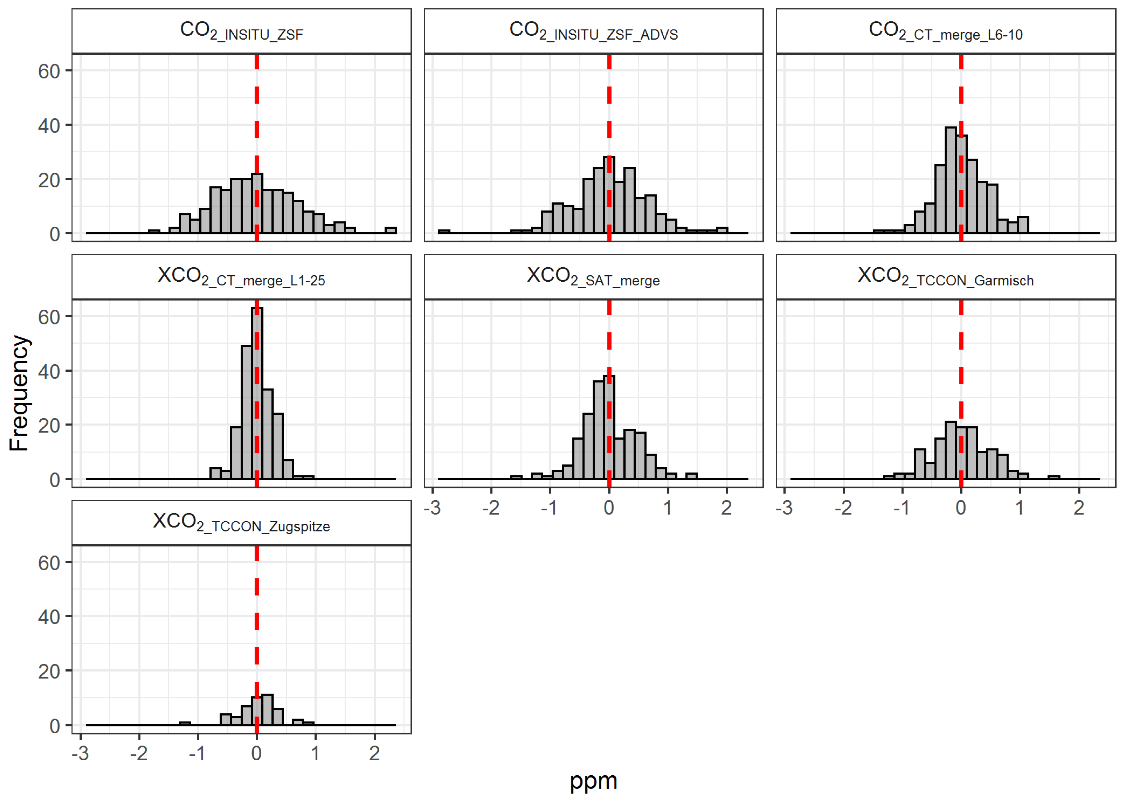
3.2. Data Processing

In order to derive the most representative background CO₂ levels for the lower free troposphere from the CO_{2_INSITU_ZSF} data set, the data selection method ADVS (Adaptive Diurnal minimum Variation Selection) was applied, which has been proven to be valid for European elevated mountain stations [7], and for long-term continuous measurements [22]. With a nighttime starting selection time window statistically identified based on data variability, the ADVS method selects the best appropriate CO₂ data on a daily basis. The selection threshold criterion at ZSF was set to no more than 0.3 ppm (standard deviation) within a 6-hour time window (22:00–03:00 local time). In total, 14.0% of validated 30-min CO₂ data were selected.

For all monthly averaged data sets, cubic spline interpolation was applied to fill missing values in the time-series, mainly for XCO_{2_SAT_Obs4MIPs} during winter periods (mostly December and January) due to poor data quality (e.g., cloudiness, shadows, or other factors). Subsequently, all CO₂ time-series were decomposed into trend, seasonal, and remainder components for further analysis using Seasonal and Trend decomposition using Loess (STL) [32]. The STL method applies the moving average technique in an inner loop with seasonal and trend smoothers based on Locally Estimated Scatterplot Smoothing (Loess), and an outer loop weighting the fitted values for the next run of smoothing until convergence is reached [33]. The smoothing parameters $s.window=5years$ and $t.window=25months$ were chosen for the seasonal and trend components, respectively. A periodic window for seasonal extraction was tested and the result was similar. The remainder of the components were assessed for all records, but no systematic signals were detected, indicating reliable decomposed results for further analysis (see Figure A1). The STL-decomposed trend and seasonal components were combined and are shown as curve fitting for all CO₂/XCO₂ time-series.

3.3. Data Analysis

The CO₂ annual growth rate was calculated from the STL-decomposed trend component based on the definition by NOAA [2], following the instructions in Buchwitz et al. [27]. For each month, we calculated the difference in CO₂ or XCO₂ between this month and the same month from the previous year. Thus, 12 values were calculated for each year. Then, the mean annual growth rate was considered as the mean of these 12 differences. The mean annual growth rates were further used for correlation analysis by Pearson’s product moment correlation, with error bars defined by the 95% confidence intervals calculated from averaging the 12 values in each year.

However, the seasonal cycle was determined from the STL-decomposed seasonal component with the seasonal amplitude calculated from the monthly maximum minus the monthly minimum of the year. The calculation method of seasonal amplitude has been compared with the curve fitting technique, by Lindqvist et al. [34] applying a skewed sine wave for the seasonal cycle, resulting in the same values. More details can be found in the Appendix A.

All data processing, analyses, and visualizations in this study were done under R programming environment (version 3.6.0) [35], with the implemented packages data.table [36], openair [37], zoo [38], ggplot2 [39], leaflet [40], mapview [41], grid [35], and gridExtra [42].

4. Results

This section first reports the complete CO₂ time-series compared. Then, the results of STL decomposition are shown with inter-annual variations of annual growth rates and seasonal cycles. A statistical summary can be found in

Table A1. Statistical summary of all CO₂ and XCO₂ data sets in this study.

Measurement Technique	Offset from CO2_insitu_ZSF (ppm ± 95% CI)	Mean Annual Growth Rate (ppm yr−1 ± 95% CI)	Mean Seasonal Amplitude (ppm ± 95% CI)
CO2_INSITU_ZSF	−	2.18 ± 0.10	13.08 ± 0.52
CO2_INSITU_ZSF_ADVS	−0.66 ± 0.15	2.20 ± 0.09	10.93 ± 0.45
CO2_CT_merge_L6-10	0.01 ± 0.17	2.21 ± 0.06	11.05 ± 0.28
XCO2_CT_merge_L1-25	−2.36 ± 0.32	2.15 ± 0.04	6.36 ± 0.18
XCO2_SAT_merge	−1.17 ± 0.38	2.13 ± 0.06	6.94 ± 0.22
XCO2_TCCON_Garmisch	−1.95 ± 0.43	2.33 ± 0.08	6.58 ± 0.19
XCO2_TCCON_Zugspitze	−1.03 ± 1.01	2.48 ± 0.16	5.22 ± 0.14

.

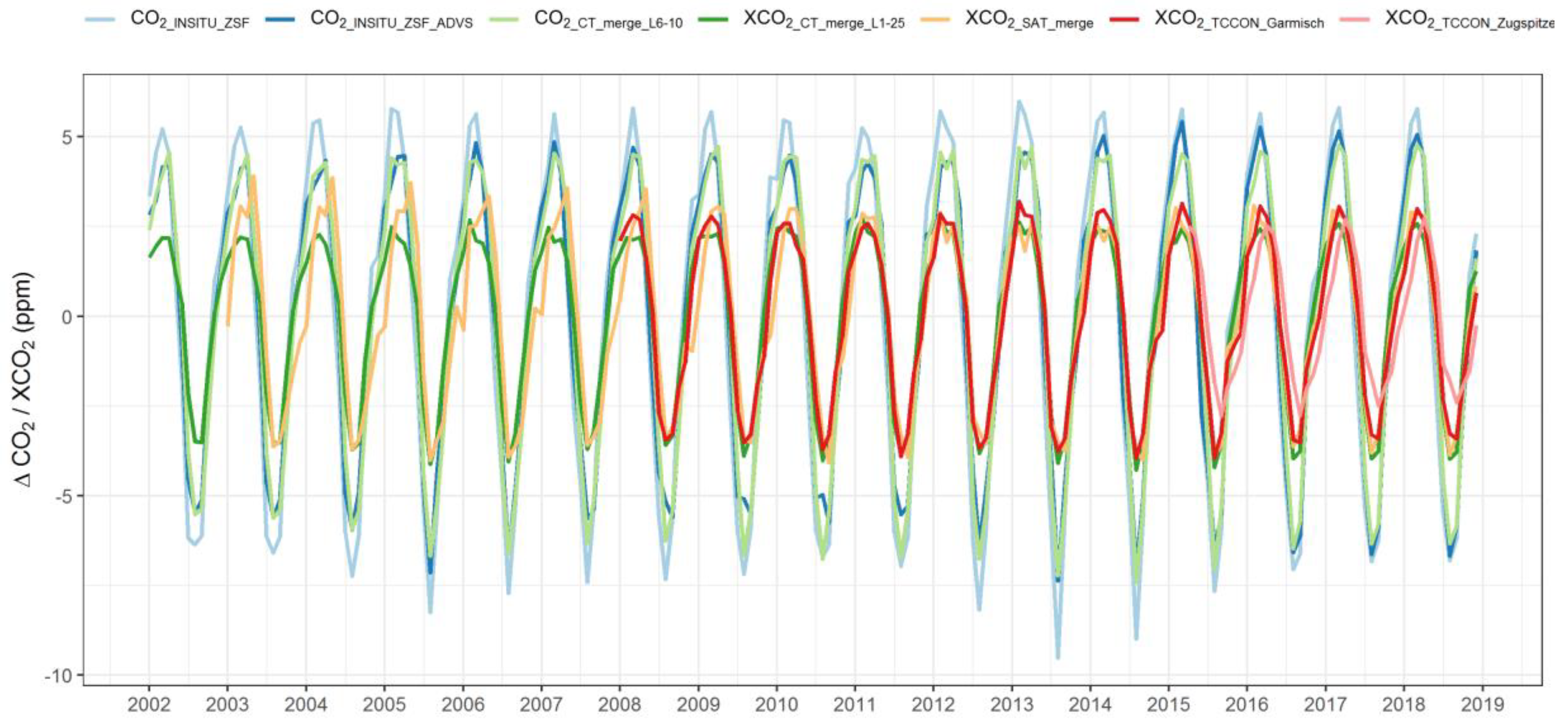
4.1. Time-Series of CO₂ and XCO₂

The atmospheric CO₂ and XCO₂ mole fractions from all measurement data sets, including the ADVS-selected surface in-situ time-series CO_{2_INSITU_ZSF_ADVS}, are given in Figure 2. All time-series are plotted in monthly resolution, together with the fitted curves that are integrated from STL-decomposed trend and seasonal components. CO_{2_INSITU_ZSF}, CO_{2_INSITU_ZSF_ADVS}, CO_{2_CT_merge_L6-10}, and XCO_{2_CT_merge_L1-25} covered the complete time period 2002–2018. The first year 2002 was missing for XCO_{2_SAT_merge}, while XCO_{2_TCCON_Garmisch} and XCO_{2_TCCON_Zugspitze} started comparatively later, in 2008 and 2015, respectively. In general, the CarbonTracker-modeled free tropospheric time-series CO_{2_CT_merge_L6-10} agreed well with the continuous in-situ measurements (both CO_{2_INSITU_ZSF} and CO_{2_INSITU_ZSF_ADVS}). However, CO_{2_INSITU_ZSF} more frequently exhibited CO₂ concentrations outside the curve fitting and thus represented the local and regional influences, e.g., higher CO₂ concentrations in 2008–2009, 2012–2013, and 2018; lower values in 2013–2014. At the same time, ADVS data selection performed effectively to exclude most of the extreme mean monthly concentrations, except for the lower value in 2005. CO_{2_INSITU_ZSF_ADVS} was still more similar in the STL-decomposed trend and seasonal fit to CO_{2_CT_merge_L6-10} than the original CO_{2_INSITU_ZSF} series.

Regarding column-averaged measurements, there were far less variations in the time-series compared to the surface measurements, since they are representative of the mean CO₂ levels of the whole vertical atmospheric concentration distribution and not only of the surface concentration as the in-situ measurements. The satellite time-series XCO_{2_SAT_merge} was slightly higher compared to the point measurements XCO_{2_TCCON_Garmisch} and XCO_{2_TCCON_Zugspitze}, while the CarbonTracker-modeled column averages XCO_{2_CT_merge_L1-25} showed the opposite. Such deviations could be attributed to differences in the representativeness of the grid values. Unlike TCCON measurements, XCO₂ values averaged from the centered and surrounding grids had the tendency to show a mean XCO₂ level from a much more regional perspective. Additionally, the extracted modeled grid for XCO_{2_CT_merge_L1-25} could potentially cover more vegetation signals that were dominant at lower elevations in the Alpine regions nearby. Additionally, it should be noted that the monthly averages for all XCO₂ measurements might not identically indicate the concentrations for the exact same days.

Figure 3 shows the offsets of all six data sets with respect to the continuous in-situ ZSF data set (CO_{2_INSITU_ZSF}), based on the monthly fitted curves. The offsets ranged from −5 to 5 ppm with bimodal distributions. All time-series exhibited negative values for the mean monthly differences relative to CO_{2_INSITU_ZSF} ranging from −0.66 ± 0.15 ppm (CO_{2_INSITU_ZSF_ADVS}) to −2.36 ± 0.32 ppm (XCO_{2_CT_merge_L1-25}), except for CO_{2_CT_merge_L6-10}, which showed a positive difference of 0.01 ± 0.17 ppm (see Table A1).

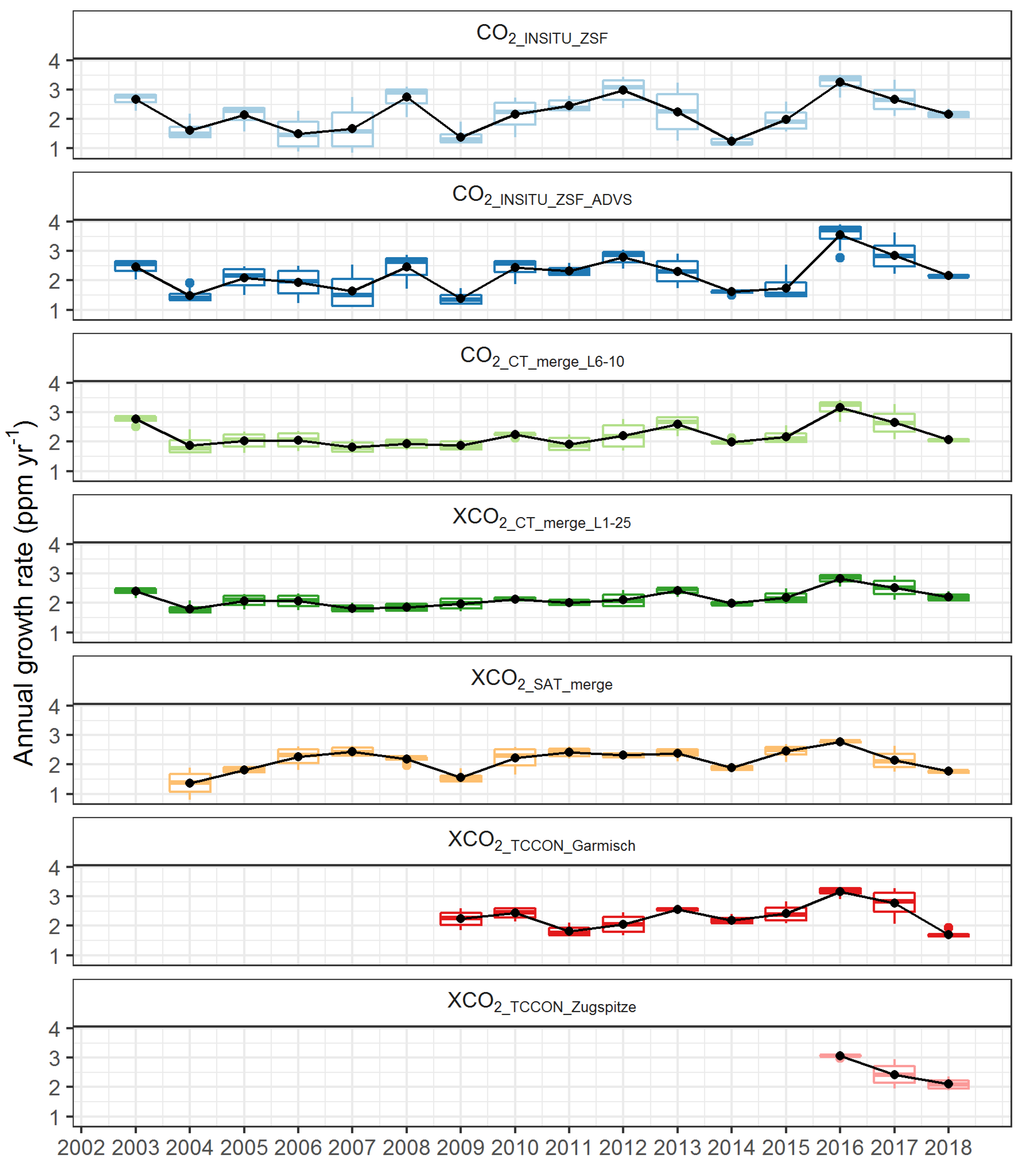
4.2. Annual Growth Rates

Apart from absolute CO₂ levels, trend analysis is always considered a more promising measure for the comparison of CO₂ time-series, i.e., for assessing whether similar year-to-year increases and inter-annual variations in CO₂ can be detected. The annual CO₂ growth rates are shown as boxplots, together with the mean growth rates connected as lines in Figure 4.

The overall mean annual growth rates of CO_{2_INSITU_ZSF} (2.18 ± 0.10 ppm yr⁻¹), CO_{2_INSITU_ZSF_ADVS} (2.20 ± 0.09 ppm yr⁻¹), and CO_{2_CT_merge_L6-10} (2.21 ± 0.06 ppm yr⁻¹) over 2002–2018 exhibited similar values around 2.2 ppm yr⁻¹ for the free troposphere, while XCO_{2_CT_merge_L1-25} and XCO_{2_SAT_merge} (starting 2003) for the total column of the atmosphere increased at slightly lower rates of 2.15 ± 0.04 ppm yr⁻¹ and 2.13 ± 0.06 ppm yr⁻¹, respectively. Due to the late start of TCCON, significantly higher annual growth rates were observed, namely 2.33 ± 0.08 ppm yr⁻¹ (Garmisch, starting in 2008) and 2.48 ± 0.16 ppm yr⁻¹ (Zugspitze, starting in 2015).

4.3. Seasonal Amptliudes

Seasonal cycles of all CO₂ and XCO₂ time-series were analyzed in regards to whether they followed comparable annual fluctuations and to identify reasons for potential discrepancies. Clear differences were found between continuous in-situ and column-averaged measurements in the mean seasonal peak-to-peak amplitudes, i.e., annual averages of monthly maximum minus monthly minimum, which were calculated from the STL-decomposed seasonal components shown in Figure 5. The largest mean seasonal amplitude of 13.08 ± 0.52 ppm was calculated for CO_{2_INSITU_ZSF}, indicating a high relevance of local influences at the measurement site. In contrast, the ADVS-selected data set (CO_{2_INSITU_ZSF_ADVS}, 10.93 ± 0.45 ppm) agreed well with the modeled CO₂ levels for the free troposphere (CO_{2_CT_merge_L6-10}, 11.05 ± 0.28 ppm), supporting a good performance of the CarbonTracker model in simulating the surface/free tropospheric CO₂ mole fractions. In this circumstance, an estimation of around 2.0 ppm mole fractions of atmospheric CO₂ is assumed to be associated with short-range carbon sources and sinks.

5. Discussion

The atmospheric CO₂ and XCO₂ mole fractions from all measurement data sets were collected and compared (see Figure 2). The differences between FTIR column observations and continuous in-situ measurements (−1.95 ± 0.43 ppm for XCO_{2_TCCON_Garmisch}, and −1.03 ± 1.01 ppm for XCO_{2_TCCON_Zugspitze}) were smaller than those found in previous studies, where differences of up to 8% have been reported [20]. This may be explained by the fact that our TCCON column observations were calibrated to World Meteorological Organization (WMO) scale, while the cited column observations were not. Furthermore, the column observations by Schibig et al. [16], showing a difference of 13 ppm with respect to surface measurements at the Jungfraujoch, were performed in the mid-infrared, not in the near-infrared as our TCCON observations. In this context, we note that Buschmann et al. [30] showed that the sensitivity of mid-infrared CO₂ column retrievals is a factor of two lower in the troposphere compared to TCCON-type near-infrared retrievals used in our study.

5.1. Inter-Annual Variation in Trend

The STL-decomposed trend components were calculated into annual CO₂ growth rates and overall mean growth rates (see Figure 4). These results perfectly matched those found by Buchwitz et al. [27], who showed a mean difference between the satellite-derived and NOAA CO₂ surface observation annual mean growth rates of 0.0 ± 0.3 ppm yr⁻¹ (± 1 standard deviation). Their reported “record-large” growth rate over 2015–2016 of around 3 ppm yr⁻¹ due to an El Niño event [43,44,45] was also clearly observed in all series of our study (ranging from 2.77 to 3.56 ppm yr⁻¹).

Equally, inter-annual variations in the annual growth rates were similar for the different CO₂ series. The continuous in-situ measurements (CO_{2_INSITU_ZSF} and CO_{2_INSITU_ZSF_ADVS}) and CarbonTracker free tropospheric model (CO_{2_CT_merge_L6-10}) agreed well, starting with a noticeably high annual growth rate in 2003 and a decreasing period from 2016 to 2018. They only differed considerably in 2008 and 2009, i.e., both CO_{2_INSITU_ZSF} and CO_{2_INSITU_ZSF_ADVS}, but not CO_{2_CT_merge_L6-10}, which showed high variations in the annual growth rates. Interestingly, also XCO_{2_SAT_merge} showed this pattern, which might again be attributed to the different spatiotemporal smoothing in the model and satellite grids compared to the local surface measurements. Especially for the period 2004–2009, it is clear that the annual growth rates in CO_{2_CT_merge_L6-10} remained stable and the same is true for XCO_{2_CT_merge_L1-25}.

Regarding column-averaged measurements, smaller variables were expected for the annual growth rates, as shown in Figure 4. Despite much shorter TCCON time-series, the decreasing trends from 2016 to 2018 were still observed in all column-averaged time-series. In 2014, a comparably lower mean annual CO₂ growth rate was depicted across all time-series. Moreover, while the 12 values tended to vary largely in 2017, they did not in 2016 and 2018. Again, this was a result consistent for all seven data sets. However, an increase in growth rates in XCO_{2_SAT_merge} from 2003 to 2007 was not seen elsewhere and thus still remains unclear. However, in general, annual growth rates agreed well among all CO₂ series, particularly in the second half of the study period, and further research should be dedicated to the differences before 2010.

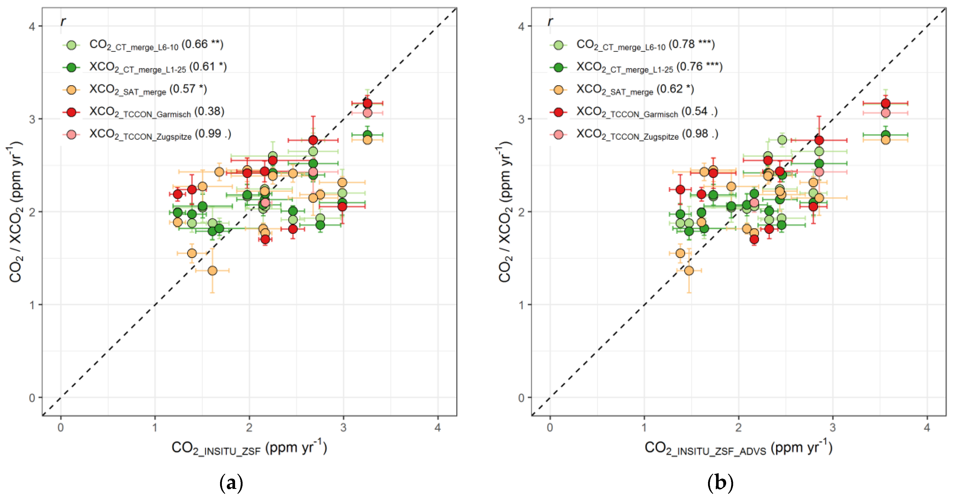
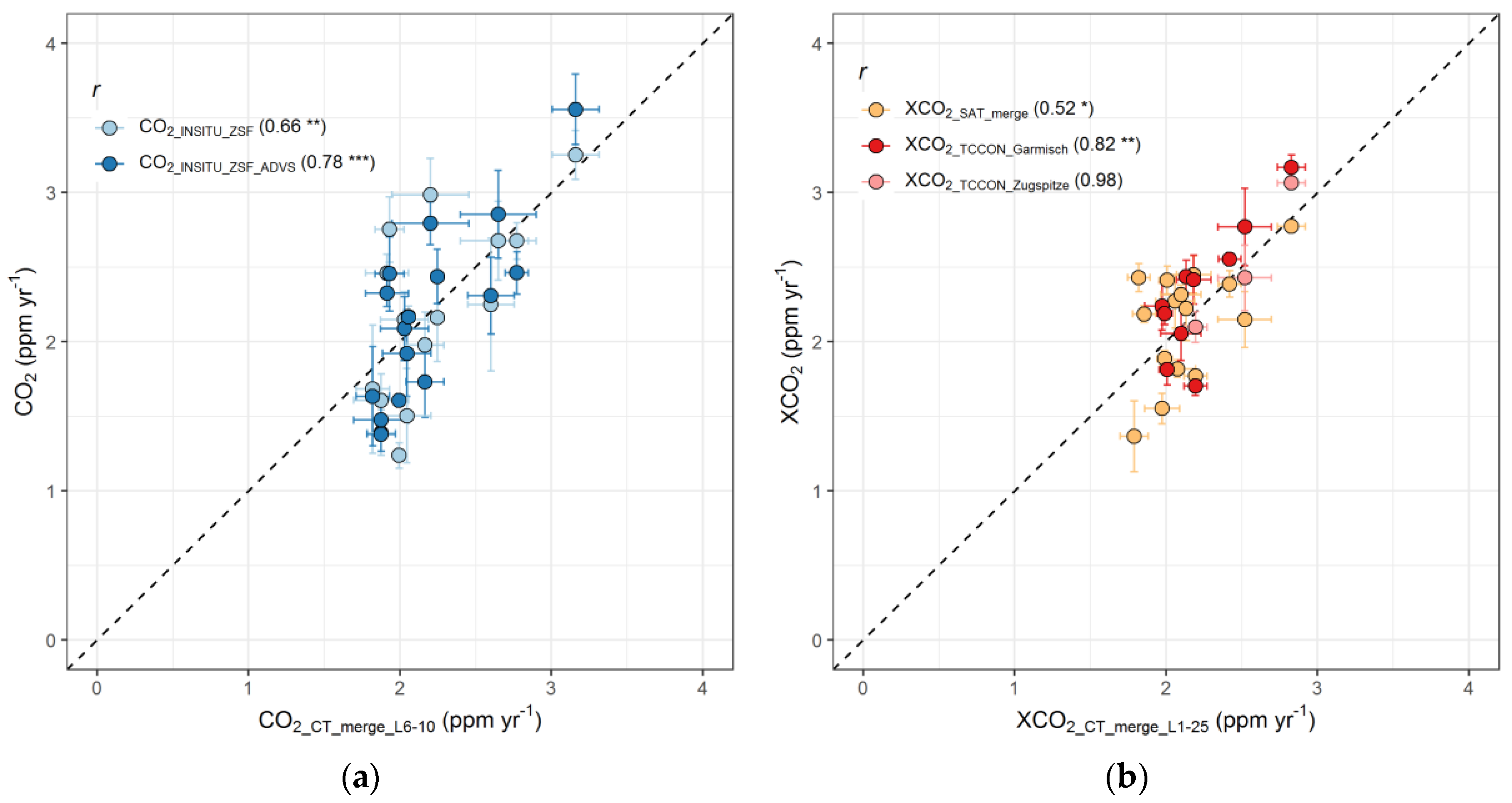
5.2. Correlation of Annual Growth Rates

Figure 6 summarizes correlations of each measurement data set with CO_{2_INSITU_ZSF} and CO_{2_INSITU_ZSF_ADVS}. The ADVS data selection intends to derive more representative CO₂ levels for a broader region, which proved to be valid since the correlation coefficients to CO_{2_INSITU_ZSF_ADVS} were higher than the respective ones to CO_{2_INSITU_ZSF}, e.g., correlation of XCO_{2_TCCON_Garmisch} growth rates to CO_{2_INSITU_ZSF_ADVS} of 0.54 (significant at 0.1 level) instead of 0.38 to CO_{2_INSITU_ZSF} (not significant). Furthermore, the CarbonTracker models also showed improved correlations from 0.66 to 0.78 with improved significance levels (0.01 to 0.001) for CO_{2_CT_merge_L6-10}, and from 0.61 to 0.76 for XCO_{2_CT_merge_L1-25} when applying the ADVS technique. A slight increase (0.57 to 0.62 at 0.05 of the significance level) is also seen for XCO_{2_sat_merge}, while the highest correlation coefficients of almost 1 were seen for XCO_{2_TCCON_Zugspitze} in both pairs, however, due to a correlation of three points from only 2015 to 2018, this is not comparable. In short, the overall improvements in the correlation coefficients were clearly recognized in all data sets with continuous in-situ measurements at ZSF after ADVS data selection, suggesting a good accordance with the background levels in the atmosphere. Interestingly, the modeled column time-series correlated better with the surface measurements in terms of the trend compared to other column-averaged measurements. Nevertheless, correlations between CO_{2_CT_merge_L6-10} and continuous in-situ measurements as well as between XCO_{2_CT_merge_L1-25} and column-averaged measurements are also provided (see Figure A2) and especially show a good correlation coefficient (0.82 **) between XCO_{2_TCCON_Garmisch} and the modeled column data set.

The levels of correlation coefficients were comparable with similar studies. Buchwitz et al. [27] reported a correlation coefficient of 0.82 between the satellite-derived growth rates and the NOAA global growth rates over 2003–2016. This higher value is assumed to be due to the global averaging effect, while our results show a more specific signature of the Zugspitze region. Equally, Schibig et al. [16] reported that correlations between the FTIR and in-situ NDIR measurements, both with and without seasonality, reached 0.82 as well.

5.3. Seasonality

The mean seasonal amplitudes of column-averaged measurements were only about one half of the amplitudes of in-situ measurements (see Figure 5). It is noteworthy that this factor-of-two amplitude reduction for column-based data sets was nicely reproduced by CarbonTracker, when comparing CO_{2_CT_merge_L6-10} with CO_{2_CT_merge_L1-25} (6.36 ± 0.18 ppm). A similar effect was also reported by Olsen and Randerson [15] for individual NOAA sites in the Northern Hemisphere. The satellite time-series had seasonal amplitudes of 6.94 ± 0.22 ppm from 2003 to 2018, while 6.58 ± 0.19 ppm was calculated for XCO_{2_TCCON_Garmisch} during 2008–2018. Finally, XCO_{2_TCCON_Zugspitze} exhibited the lowest mean seasonal amplitude of 5.22 ± 0.14 ppm for the last four years (2015–2018). Taking the same period for the TCCON Garmisch site, the mean seasonal amplitude was still significantly higher (6.64 ± 0.50 ppm for XCO_{2_TCCON_Garmisch} during 2015–2018). Therefore, an amplitude difference of around 1.5 ppm can be attributed mainly to the carbon sinks from photosynthesis in the relatively lower elevations of the Zugspitze region compared to the TCCON Zugspitze site (from both the TCCON Garmisch site and the satellite grid coverage perspectives).

In addition, due to different vertical mixing and amounts of air masses measured at the surface or in the column, changes in phase (i.e., timing of seasonal peaks) are expected to be observed as well [7,22]. Olsen and Randerson [15] suggested that the phase delay between surface and column measurements can be up to seven weeks regarding the timing of seasonal maximum and minimum, while Lindqvist et al. [34] showed an up to two–three weeks difference regarding the maximum at the European sites with a smaller difference for the minimum of less than six days. From our study, given that monthly time-series were used, only the shifts in month could be derived here. On average, one–two-month delays were detected in monthly maxima from all column measurements compared to CO_{2_INSITU_ZSF}, especially in the first half of the satellite time-series (XCO_{2_SAT_merge}, 2003–2008). Interestingly, the seasonal amplitudes during this period of XCO_{2_SAT_merge} also differed greatly from the remaining latter half (2009–2018). This could be probably explained by the fact that the TANSO-FTS/GOSAT satellite measurements included in this merged product (XCO_{2_SAT_Obs4MIPs}) only started from 2009. In opposition to this, delays of one month at the most can be found for seasonal minima mainly from satellite and TCCON measurements.

At last, inter-annual changes in the seasonality were detected more clearly for continuous in-situ measurements than for the column-averaged measurements, which is in accordance with the anomalies described in Section 4.1. However, some other seasonal patterns are still worthy of further investigations. A slight “shoulder” behavior could be observed for all time-series, usually around November and December, suggesting a slower CO₂ increase during this period. Such a “pause” cannot be fully understood yet, but is probably associated with a known, relatively regular winter warming effect (named “Christmas-thaw weather” over Europe). Meanwhile, the seasonal decrease from monthly maximum to monthly minimum tended to vary rapidly over time, indicating the great influences from vegetation photosynthesis as the carbon sinks during spring to summertime. Such a pattern should be described more precisely in seasonal modeling in the future.

6. Conclusions

This study compared surface CO₂ measurements with column-averaged measurements at a specific site in Southern Germany. Continuous in-situ CO₂ measurements from 2002 to 2018 at Zugspitze–Schneefernerhaus were used and selected by the data selection method ADVS in order to obtain more representative background levels for a broader region. In order to compare with ground-based FTIR measurements, two TCCON sites, Garmisch and Zugspitze, were chosen at the nearby locations. In addition to providing more comparable results over the region, satellite measurements were included by defining selected grids centered at the specific Zugspitze site. At last, the simulated CO₂ mole fractions from the CarbonTracker models were included and validated for other measurements.

The mean offsets of satellite and FTIR measurements from the continuous in-situ measurements were less than 2.0 ppm, showing generally good agreements. By decomposing each CO₂ time-series into trend, seasonal, and remainder components, the annual growth rates and seasonal amplitudes were compared. Fluctuations of the mean annual growth rates were consistent over the time period, proving that both continuous in-situ and column-averaged measurements are able to capture the CO₂ trend effectively in the atmosphere. The correlation analysis showed lower correlation coefficients than other global studies due to the site-specific focus of this study. However, differences in seasonal cycles were clear with respect to both amplitudes and phases. Column-averaged measurements exhibited smaller seasonal amplitudes and clearly delayed phases regarding both seasonal maximum and minimum. This is most likely due to lessened influences from the local to regional scale as well as to a time lag by the vertical mixing of greater amounts of air masses in the column profile.

With respect to the research questions, the study clearly showed that different types of CO₂ measurements/time-series are comparable by applying a consistent data processing routine. The main differences between continuous in-situ and column-averaged measurements were detected in the seasonal amplitudes, supporting the essential distinction of the measuring objects. However, potential errors should always be noted, especially regarding both temporal and spatial resolutions. Such a comparison provides the basis for a better understanding of these two different types of measurements and is helpful for improved data integration in further research.

References

1. IPCC. Climate Change 2014: Synthesis Report. In Contribution of Working Groups I, II and III to the Fifth Assessment Report of the Intergovernmental Panel on Climate Change; Pachauri, R.K., Meyer, L.A., Eds.; Core Writing Team: Geneva, Switzerland, 2014; p. 151. ISBN 978-929-169-143-2. [Google Scholar]
2. Dlugokencky, E.; Tans, P. Trends in Atmospheric Carbon Dioxide. NOAA/ESRL. Available online: www.esrl.noaa.gov/gmd/ccgg/trends/ (accessed on 21 October 2019).
3. Schultz, M.G.; Akimoto, H.; Bottenheim, J.; Buchmann, B.; Galbally, I.E.; Gilge, S.; Helmig, D.; Koide, H.; Lewis, A.C.; Novelli, P.C.; et al. The Global Atmosphere Watch reactive gases measurement network. Elem. Sci. Anthr. 2015, 3. [Google Scholar] [CrossRef] [Green Version]
4. Toon, G.; Blavier, J.; Washenfelder, R.; Wunch, D.; Keppel-Aleks, G.; Wennberg, P.; Connor, B.; Sherlock, V.; Griffith, D.; Deutscher, N.; et al. Total Column Carbon Observing Network (TCCON). In Advances in Imaging, OSA Technical Digest (CD). Opt. Soc. Am. 2009, JMA3. [Google Scholar] [CrossRef] [Green Version]
5. Hamazaki, T.; Kaneko, Y.; Kuze, A.; Kondo, K. Fourier transform spectrometer for Greenhouse Gases Observing Satellite (GOSAT). Enabling Sens. Platf. Technol. Spaceborne Remote Sens. 2005, 5659, 73–80. [Google Scholar] [CrossRef]
6. Crisp, D. Measuring atmospheric carbon dioxide from space with the Orbiting Carbon Observatory-2 (OCO-2). Earth Obs. Syst. 2015, 9607, 960702. [Google Scholar] [CrossRef]
7. Yuan, Y.; Ries, L.; Petermeier, H.; Steinbacher, M.; Gómez-Peláez, A.J.; Leuenberger, M.C.; Schumacher, M.; Trickl, T.; Couret, C.; Meinhardt, F.; et al. Adaptive selection of diurnal minimum variation: A statistical strategy to obtain representative atmospheric CO2 data and its application to European elevated mountain stations. Atmos. Meas. Tech. 2018, 11, 1501–1514. [Google Scholar] [CrossRef] [Green Version]
8. Fang, S.X.; Zhou, L.X.; Tans, P.P.; Ciais, P.; Steinbacher, M.; Xu, L.; Luan, T. In situ measurement of atmospheric CO2 at the four WMO/GAW stations in China. Atmos. Chem. Phys. 2014, 14, 2541–2554. [Google Scholar] [CrossRef] [Green Version]
9. Hernández-Paniagua, I.Y.; Lowry, D.; Clemitshaw, K.C.; Fisher, R.E.; France, J.L.; Lanoisellé, M.; Ramonet, M.; Nisbet, E.G. Diurnal, seasonal, and annual trends in atmospheric CO2 at southwest London during 2000–2012: Wind sector analysis and comparison with Mace Head, Ireland. Atmos. Environ. 2015, 105, 138–147. [Google Scholar] [CrossRef]
10. Burrows, J.P.; Hölzle, E.; Goede, A.P.H.; Visser, H.; Fricke, W. SCIAMACHY—scanning imaging absorption spectrometer for atmospheric chartography. Acta Astronaut. 1995, 35, 445–451. [Google Scholar] [CrossRef]
11. Bovensmann, H.; Burrows, J.P.; Buchwitz, M.; Frerick, J.; Noël, S.; Rozanov, V.V.; Chance, K.V.; Goede, A.P.H. SCIAMACHY: Mission Objectives and Measurement Modes. J. Atmos. Sci. 1999, 56, 127–150. [Google Scholar] [CrossRef] [Green Version]
12. Aumann, H.H.; Miller, C.R. Atmospheric infrared sounder (AIRS) on the earth observing system. Adv. Next Gener. Satell. 1995, 2583, 332–343. [Google Scholar] [CrossRef]
13. Miao, R.; Lu, N.; Yao, L.; Zhu, Y.; Wang, J.; Sun, J. Multi-Year Comparison of Carbon Dioxide from Satellite Data with Ground-Based FTS Measurements (2003–2011). Remote Sens. 2013, 5, 3431–3456. [Google Scholar] [CrossRef] [Green Version]
14. Liang, A.; Gong, W.; Han, G.; Xiang, C. Comparison of Satellite-Observed XCO2 from GOSAT, OCO-2, and Ground-Based TCCON. Remote Sens. 2017, 9, 1033. [Google Scholar] [CrossRef] [Green Version]
15. Olsen, S.C.; Randerson, J.T. Differences between surface and column atmospheric CO2 and implications for carbon cycle research. J. Geophys. Res. 2004, 109, 419. [Google Scholar] [CrossRef] [Green Version]
16. Schibig, M.F.; Mahieu, E.; Henne, S.; Lejeune, B.; Leuenberger, M.C. Intercomparison of in situ NDIR and column FTIR measurements of CO2 at Jungfraujoch. Atmos. Chem. Phys. 2016, 16, 9935–9949. [Google Scholar] [CrossRef] [Green Version]
17. Shim, C.; Lee, J.; Wang, Y. Effect of continental sources and sinks on the seasonal and latitudinal gradient of atmospheric carbon dioxide over East Asia. Atmos. Environ. 2013, 79, 853–860. [Google Scholar] [CrossRef]
18. Nalini, K.; Uma, K.N.; Sijikumar, S.; Tiwari, Y.K.; Ramachandran, R. Satellite- and ground-based measurements of CO2 over the Indian region: Its seasonal dependencies, spatial variability, and model estimates. Int. J. Remote Sens. 2018, 39, 7881–7900. [Google Scholar] [CrossRef]
19. Sánchez, M.L.; Pérez, I.A.; Buchwitz, M.; García, M.A. XCO2 SCIAMACHY Total Column and CO2 Ground Inter-comparison Results in the Spanish Plateau. In Proceedings of the ESA Living Planet Symposium, Bergen, Norway, 28 June–2 July 2010; Lacoste-Francis, H., Ed.; ESA Communications: Noordwijk, The Netherlands, 2010; ISBN 978-929-221-250-6. [Google Scholar]
20. Warneke, T.; Yang, Z.; Olsen, S.; Körner, S.; Notholt, J.; Toon, G.C.; Velazco, V.; Schulz, A.; Schrems, O. Seasonal and latitudinal variations of column averaged volume-mixing ratios of atmospheric CO2. Geophys. Res. Lett. 2005, 32, L03808. [Google Scholar] [CrossRef] [Green Version]
21. Warneke, T.; Petersen, A.K.; Gerbig, C.; Jordan, A.; Rödenbeck, C.; Rothe, M.; Macatangay, R.; Notholt, J.; Schrems, O. Co-located column and in situ measurements of CO2 in the tropics compared with model simulations. Atmos. Chem. Phys. 2010, 10, 5593–5599. [Google Scholar] [CrossRef] [Green Version]
22. Yuan, Y.; Ries, L.; Petermeier, H.; Trickl, T.; Leuchner, M.; Couret, C.; Sohmer, R.; Meinhardt, F.; Menzel, A. On the diurnal, weekly, and seasonal cycles and annual trends in atmospheric CO2 at Mount Zugspitze, Germany, during 1981–2016. Atmos. Chem. Phys. 2019, 19, 999–1012. [Google Scholar] [CrossRef] [Green Version]
23. Wunch, D.; Toon, G.C.; Blavier, J.F.L.; Washenfelder, R.A.; Notholt, J.; Connor, B.J.; Griffith, D.W.T.; Sherlock, V.; Wennberg, P.O. The total carbon column observing network. Philos. Trans. A Math. Phys. Eng. Sci. 2011, 369, 2087–2112. [Google Scholar] [CrossRef] [Green Version]
24. Sussmann, R.; Schäfer, K. Infrared spectroscopy of tropospheric trace gases: Combined analysis of horizontal and vertical column abundances. Appl. Opt. 1997, 36, 735–741. [Google Scholar] [CrossRef] [PubMed]
25. Sussmann, R.; Rettinger, M. TCCON Data from Zugspitze (DE), Release GGG2014.R1 [Data set]. CaltechDATA 2018, r1. [Google Scholar] [CrossRef]
26. Sussmann, R.; Rettinger, M. TCCON data from Garmisch (DE), Release GGG2014.R2 [Data set]. CaltechDATA 2018, r2. [Google Scholar] [CrossRef]
27. Buchwitz, M.; Reuter, M.; Schneising, O.; Noël, S.; Gier, B.; Bovensmann, H.; Burrows, J.P.; Boesch, H.; Anand, J.; Parker, R.J.; et al. Computation and analysis of atmospheric carbon dioxide annual mean growth rates from satellite observations during 2003–2016. Atmos. Chem. Phys. 2018, 18, 17355–17370. [Google Scholar] [CrossRef] [Green Version]
28. Crisp, D.; Pollock, H.R.; Rosenberg, R.; Chapsky, L.; Lee, R.A.M.; Oyafuso, F.A.; Frankenberg, C.; O’Dell, C.W.; Bruegge, C.J.; Doran, G.B.; et al. The on-orbit performance of the Orbiting Carbon Observatory-2 (OCO-2) instrument and its radiometrically calibrated products. Atmos. Meas. Tech. 2017, 10, 59–81. [Google Scholar] [CrossRef] [Green Version]
29. Peters, W.; Jacobson, A.R.; Sweeney, C.; Andrews, A.E.; Conway, T.J.; Masarie, K.; Miller, J.B.; Bruhwiler, L.M.P.; Pétron, G.; Hirsch, A.I.; et al. An atmospheric perspective on North American carbon dioxide exchange: CarbonTracker. Proc. Natl. Acad. Sci. USA 2007, 104, 18925–18930. [Google Scholar] [CrossRef] [Green Version]
30. Buschmann, M.; Deutscher, N.M.; Sherlock, V.; Palm, M.; Warneke, T.; Notholt, J. Retrieval of XCO2 from ground-based mid-infrared (NDACC) solar absorption spectra and comparison to TCCON. Atmos. Meas. Tech. 2016, 9, 577–585. [Google Scholar] [CrossRef] [Green Version]
31. Berrisford, P.; Dee, D.P.; Poli, P.; Brugge, R.; Fielding, M.; Fuentes, M.; Kållberg, P.W.; Kobayashi, S.; Uppala, S.; Simmons, A. The ERA-Interim archive Version 2.0. ERA Report, ECMWF. 2011, p. 23. Available online: https://www.ecmwf.int/node/8174 (accessed on 31 October 2019).
32. Cleveland, R.B.; Cleveland, W.S.; McRae, J.E.; Terpenning, I. STL: A seasonal-trend decomposition. J. Off. Stat. 1990, 6, 3–73. [Google Scholar]
33. Pickers, P.A.; Manning, A.C. Investigating bias in the application of curve fitting programs to atmospheric time series. Atmos. Meas. Tech. 2015, 8, 1469–1489. [Google Scholar] [CrossRef] [Green Version]
34. Lindqvist, H.; O’Dell, C.W.; Basu, S.; Boesch, H.; Chevallier, F.; Deutscher, N.; Feng, L.; Fisher, B.; Hase, F.; Inoue, M.; et al. Does GOSAT capture the true seasonal cycle of carbon dioxide? Atmos. Chem. Phys. 2015, 15, 13023–13040. [Google Scholar] [CrossRef] [Green Version]
35. RC Team. R: A Language and Environment for Statistical Computing; Vienna, Austria. 2014. Available online: https://www.R-project.org/ (accessed on 11 December 2019).
36. Dowle, M.; Srinivasan, A. Data. Table: Extension of ‘Data.Frame’. 2019. Available online: https://CRAN.R-project.org/package=data.table (accessed on 9 December 12).
37. Carslaw, D.C.; Ropkins, K. openair—An R package for air quality data analysis. Environ. Model. Softw. 2012, 27–28, 52–61. [Google Scholar] [CrossRef]
38. Zeileis, A.; Grothendieck, G. Zoo: S3 Infrastructure for Regular and Irregular Time Series. J. Stat. Softw. 2005, 14, 1–27. [Google Scholar] [CrossRef] [Green Version]
39. Wickham, H. Ggplot2: Elegant Graphics for Data Analysis; Springer-Verlag: New York, NY, USA, 2016; ISBN 978-331-924-277-4. [Google Scholar]
40. Cheng, J.; Karambelkar, B.; Xie, Y. Leaflet: Create Interactive Web Maps with the JavaScript ‘Leaflet’ Library. 2018. Available online: https://CRAN.R-project.org/package=leaflet (accessed on 16 November 2019).
41. Appelhans, T.; Detsch, F.; Reudenbach, C.; Woellauer, S. Mapview: Interactive Viewing of Spatial Data in R. 2019. Available online: https://CRAN.R-project.org/package=mapview (accessed on 13 May 2019).
42. Auguie, B. Gridextra: Miscellaneous Functions for “Grid” Graphics. 2017. Available online: https://CRAN.R-project.org/package=gridExtra (accessed on 9 September 2017).
43. Heymann, J.; Reuter, M.; Buchwitz, M.; Schneising, O.; Bovensmann, H.; Burrows, J.P.; Massart, S.; Kaiser, J.W.; Crisp, D. CO2 emission of Indonesian fires in 2015 estimated from satellite-derived atmospheric CO2 concentrations. Geophys. Res. Lett. 2017, 44, 1537–1544. [Google Scholar] [CrossRef]
44. Liu, J.; Bowman, K.W.; Schimel, D.S.; Parazoo, N.C.; Jiang, Z.; Lee, M.; Bloom, A.A.; Wunch, D.; Frankenberg, C.; Sun, Y.; et al. Contrasting carbon cycle responses of the tropical continents to the 2015–2016 El Niño. Science 2017, 358. [Google Scholar] [CrossRef] [Green Version]
45. Peters, G.P.; Le Quéré, C.; Andrew, R.M.; Canadell, J.G.; Friedlingstein, P.; Ilyina, T.; Jackson, R.B.; Joos, F.; Korsbakken, J.I.; McKinley, G.A.; et al. Towards real-time verification of CO2 emissions. Nat. Clim. Chang. 2017, 7, 848. [Google Scholar] [CrossRef] [Green Version]
Figure 1. Locations of GAW Global station ZSF and TCCON sites Zugspitze and Garmisch with rectangles representing the spatial coverage of XCO2 levels extracted in this study for satellite measurements (red) and CarbonTracker-modeled results (blue).
Remotesensing 11 02981 g001
Figure 2. Monthly CO2 series of all measurements/data products shown as colored points with fitted curves (colored lines) consisting of STL-decomposed trend and seasonal components, divided into CO2 (upper panel) and XCO2 (lower panel).
Remotesensing 11 02981 g002
Figure 3. Offsets of six different CO2 and XCO2 data sets of this study (monthly fitted curves, STL-decomposed trend plus seasonal components) relative to CO2_INSITU_ZSF.
Remotesensing 11 02981 g003
Figure 4. Annual mean growth rates derived from all seven CO2 and XCO2 series in this study (STL-decomposed trends, black points, and lines). Colored boxplots represent all 12 values of growth rates from monthly averages.
Remotesensing 11 02981 g004
Figure 5. Seasonal cycles from STL-decomposed seasonal components of the different CO2 and XCO2 series of this study.
Remotesensing 11 02981 g005
Figure 6. Scatter plots of annual mean growth rates from STL trend components in (a) CO2_INSITU_ZSF and (b) CO2_INSITU_ZSF_ADVS versus CO2/XCO2 from other measurement data sets. Pearson’s product-moment correlation coefficients (r) are listed accordingly for each pair. The significance levels are shown in symbols as 0.001 (***), 0.01 (**), 0.05 (*), and 0.1 (.). The 95% confidence intervals are shown as error bars on both the x and y-axis with dashed lines representing the 1:1 line.
Remotesensing 11 02981 g006