Forward and Backward Visual Fusion Approach to Motion Estimation with High Robustness and Low Cost

Abstract

We present a novel low-cost visual odometry method of estimating the ego-motion (self-motion) for ground vehicles by detecting the changes that motion induces on the images. Different from traditional localization methods that use differential global positioning system (GPS), precise inertial measurement unit (IMU) or 3D Lidar, the proposed method only leverage data from inexpensive visual sensors of forward and backward onboard cameras. Starting with the spatial-temporal synchronization, the scale factor of backward monocular visual odometry was estimated based on the MSE optimization method in a sliding window. Then, in trajectory estimation, an improved two-layers Kalman filter was proposed including orientation fusion and position fusion. Where, in the orientation fusion step, we utilized the trajectory error space represented by unit quaternion as the state of the filter. The resulting system enables high-accuracy, low-cost ego-pose estimation, along with providing robustness capability of handing camera module degradation by automatic reduce the confidence of failed sensor in the fusion pipeline. Therefore, it can operate in the presence of complex and highly dynamic motion such as enter-in-and-out tunnel entrance, texture-less, illumination change environments, bumpy road and even one of the cameras fails. The experiments carried out in this paper have proved that our algorithm can achieve the best performance on evaluation indexes of average in distance (AED), average in X direction (AEX), average in Y direction (AEY), and root mean square error (RMSE) compared to other state-of-the-art algorithms, which indicates that the output results of our approach is superior to other methods.

1. Introduction

1.1. Motivations and Technical Challenges

This paper aims at developing a visual fusion approach for online ego-motion estimation with the data from onboard forward and backward cameras. Ego-motion represents and describes the self-motion of a moving object and the ego-motion problem can be stated as the recovery of observer rotation and direction of translation by at a given instant of time, as the observer moves through the environment, which is also called ego-motion estimation. The most ego-motion estimation methods comprise two steps, motion-field computation and motion field analysis [1]. In many real-world applications, the estimation of egomotion and localization is a pivot of major vision-based navigation system especially for autonomous ground vehicle and robotics [2,3,4], since it forms the basis of subsequent scene understanding and vehicle control [5]. In addition, ego-motion estimation in vehicles and robots is fundamental as it is usually the pre-requisite for higher-layer tasks, such as robot-based surveillance, autonomous navigation, path planning, for example, References [6,7]. A vision-based odometry system, compared to a traditional wheel-based or satellites-based localization system, has the advantages of an impervious character to inherent sensor inefficacies [8,9] (e.g., wheel encoder error because of uneven, slippery terrain or other adverse conditions) and can be used in a GPS-denied area [10,11] (e.g., underwater and tunnels in urban environments.) The proposed approach utilizes only visual perception cameras with lightweight, high robustness and low-cost characters.

Visual ego-motion estimation has been successfully proven to be able to estimate the movement of a road vehicle over a long distance under certain conditions [12], with a relative error ranging from 0.1 to 2% [13]. It incrementally estimates camera poses, yet small errors are inevitably accumulated and over time the estimated ego-motion slowly drifts away from their ground true [14]. With the purpose of improving the performance, appreciable progress has been made to enhance the system robustness, accuracy and efficiency. Many efforts, such as the direct method, semi-direct method and feature-based method, have been made for different visual ego-motion formulations [15]. Global map optimization techniques like loop closure, bundle adjustment (BA) and pose graph optimization were also proposed to make better the overall performance, which adjust the estimation results by taking into account the entire observation equations and eventual constraints [16].

However, until now, it was still hard to integrate into the motion estimation application of mobile robots and even less in that of an autonomous vehicle [17]. It suffers from many limitations [18,19,20]. First, most visual odometry methods encounter the inherent imperfection of motion drift and the inner fragility of sensor degradation. The data association model of visual ego-motion estimation is not completely stable and can fail under ubiquitous noise, texture-less scenery and the different level of sensor degradation. Second, the commonly used global drift optimization method of loop closure is often out of action, especially for large-scale outdoor use. Most of the time, there is no loop in many scenarios for a moving robot or vehicle in urban areas and the computation of large loops is time consuming, which make the robustness of system even more critical. Third, as a kind of passive measurement method, the motion estimation scheme usually requires enough keypoints [12], which are difficult to detect and track in some complicated circumstance, such as enter-in-and-out tunnel entrance scenery of sudden illumination changes, resulting in an enlargement of the outliers. Very often, other types of sensors, including differential GPS, precise IMU or 3D Lidar, are integrated to improve the system capability, along with a great increase of system cost.

1.2. Literature Review

Visual odometry is a particular case of structure-from-motion (SFM) [21], which aims to incrementally estimate the egomotion of an agent (e.g., vehicle, human and robot) using only vision stream and its origins can be dated back to works such as References [22,23]. The first visual odometry systems were successfully used by NASA in their Mars exploration program, endeavoring to provide all-terrain rovers with the capability of estimating its motion in the presence of wheel slippage terrains [24]. From then on, several methods, techniques and sensor models have been developed and employed to accomplish both vehicle and robotics’ egomotion [25,26].

Some of the works were accomplished utilizing monocular vision technology with a single camera that they must measure the relative motion with 2-D bearing data [27]. Since the absolute scale is not clear, the monocular visual odometry has to calculate the relative scale and camera pose using either trifocal tensor method or the knowledge of 3-D structure [28]. Related works can generally be divided into three categories—appearance-based methods, feature-based methods and hybrid methods. Undeniably, some of them can deliver good results [29,30,31], but still they require high quality features to robustly perform and are more prone to errors [19]. Since our work is emphasizing the robust ego-motion of road vehicles in complex urban environments, the use of only a monocular vision system is not enough to meet the requirement and to alleviate the disturbances from a complex environment, including low textured scenes, non-stationary objects and others.

The idea of estimating egomotion from consecutive 3-D frames with a stereo vision method was successfully utilized in Reference [32]. A collaborative factor of these works is the utilization of feature-based methods because of the efficiency and robustness. As the works showing, both sparse features and dense features are used to establish corresponds between consecutive frames from input image sequence. Some of the most common choices are point [33], lines [34], contour [35], and hybrid [36], which can be tracked in both spatial and temporal domains. Point feature is the most commonly used of all, because of its simplicity. However, because of the complexity of dynamic road scenes, errors are unavoidable, appearing in every stage of detection, matching and tracking, especially in urban environments with texture-less, illumination change environments or bumpy road. It makes the robustness problem extremely critical.

Considering the problem of robustness, many researchers have established hypothesis-and-test and coarse-to-fine motion estimation mechanism based on the Random Sample Consensus (RANSAC) scheme, the bundle adjustment optimization approach (BA) and loop closure methods (LC). The 5-points based RANSAC algorithm for monocular visual odometry [37] and 3-points scheme for stereo method [38] has been proposed in the beginning. Yet, with the increase of complexity of environment the RANSAC iterations would grow exponentially, along with the increasing conflict of internal keypoints and the decreasing confidence of vision-based estimation results. Some other works use BA and LC methods to compensate for the drift of visual odometry once the loop is detected successful, but the absolute scale is very difficult to determine using mono based ego-motion estimation. Moreover, the paths of a moving agent do not always have loops in urban environment.

In this case, a combination of other sensors such as wheeled odometry [2], inertial sensing [18], and global position system [39] have been used. However, they have intrinsic limitations—wheeled odometry would be seriously affected in uneven, slippery terrain or other adverse conditions and prone to drift due to error accumulation. While the commonly used civil GPS can only update with a frequency of 1 Hz and the low-cost IMU is not accurate enough to fit the ego-motion estimation use. Some researchers integrated high defined maps (HDM) into the ego-motion estimation system, which can yield good results but have problems with the large-scale HDM collecting, high cost and local security laws [40]. In this work, we describe a novel visual odometry method only leveraging data from inexpensive visual sensors of forward and backward cameras, which enables high-accuracy, low-cost ego-pose estimation, along with providing robustness capability of handing camera module degradation. Moreover, different from the existing works, using only cameras instead of other sensors for computing egomotion allows a simple integration of egomotion data into other vision based algorithms, such as obstacle, pedestrian, and lane detection, without the need for calibration between sensors.

1.3. Main Contributions

We are interested in solving the ego-motion estimation with high robustness and low cost, along with solve the problem in real time and reliability. The issue is closely relevant to deal with the sensor degradation due to complex environment [41], such as illumination change, texture-less, and structure-less circumstance. To this end, in order to keep proposed approach cost competitiveness, we only leverage data from inexpensive visual sensors with different orientations. Our main contributions are summarized as follows:

(1) Utilizing the outstanding features of symmetry-adaption configuration of forward and backward cameras, we provided a new fusion mechanism of two-layers data processing to comprehensive utilize the nearby environment information. Therefore, it achieves high accuracy and low drift.

(2) The data processing pipeline was carefully designed to handle sensor degradation. Starting with the spatial-temporal synchronization, the scale factor of backward monocular visual odometry was estimated based on the MSE optimization method in sliding-window. With this help, both the forward and the backward camera own the capability of localization independently.

(3) Further, utilizing the fusion of two-layers Kalman Filter, the proposed pipeline can fully or partially bypass failure modules and make use of the rest of the pipeline to handle sensor degradation.

To the best of our knowledge, the proposed method is by far the cheapest method to enable such high robustness ego-motion estimation capable of handling sensor degradation under various lighting and structural conditions.

The remainder of this paper is organized as follows: Section 2 describes the detailed methodology including scale estimation and trajectory fusion. In Section 3, the experimental dataset, the performance evaluation results of the proposed method are presented. Section 4 and Section 5 summarize this paper and discuss future research directions.

2. Materials and Methods

2.1. Assumptions and Coordinate Systems

Considering a sensor system including forward stereo camera and backward monocular camera, we assume that ego-motion estimation model is a rigid body motion model and the above cameras can be modeled by the pinhole camera model. Then, using the Zhang method [42], the intrinsic and extrinsic parameters can be easily calibrated in advance. With the calibration matrix, the relative pose transformation matrix between two camera systems can be obtained. Hence, we can use a single coordinate system for both the forward stereo camera and the backward monocular camera. For simplicity, in the 6DoF pose calculated by the proposed method is transformed to original global coordinate. The coordinate systems are defined in the following (see Figure 1 for illustration).

There are three coordinates used in our system, the original global coordinate $\left\{G\right\}$, Forward camera coordinate system $\left\{C_F\right\}$ and Backward camera coordinate system $\left\{C_R\right\}$, which are defined as follows:

• We parallel X-O-Y plane of $\left\{G\right\}$ to the horizontal plane. The $Z_0$-axis points opposite to gravity. The $X_0$-axis points forward of the mobile platform, and the $Y_0$-axis is determined by the right-hand rule.
• Forward camera coordinate system $\left\{C_F\right\}$ is set originated at the left camera optical center of stereo camera system $\left\{O_{F1}\right\}$. The x-axis points to the left, the y-axis points upward, and the z-axis points forward coinciding with the camera principal axis.
• Backward camera coordinate system $\left\{C_R\right\}$ is originated at the camera optical center of monocular camera system $\left\{O_R\right\}$. The x-axis points to the left, the y-axis points upward, and the z-axis points forward coinciding with the camera principal axis.

2.2. Data Association of Forward-Facing and Backward-Facing Cameras

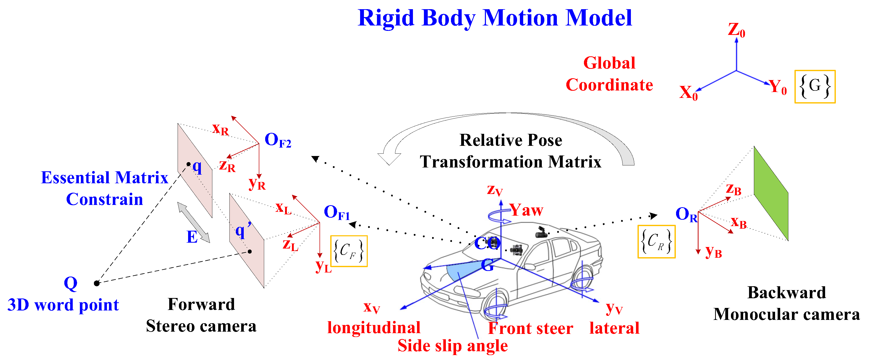
With the purpose of fitting and fusing the data of a backward-facing monocular camera and forward-facing stereo camera, the key point of data synchronization both in spatial and temporal space must be solved beforehand, which is shown Figure 2.

Within the stereo camera, left frame and right frame are triggered at the same time by the hardware flip-flop circuit. Then, we can assume that they were hardware synchronized and have the same timestamps. Hence, we only need to synchronize the data between monocular camera and stereo camera both in spatial and temporal space.

Using the camera intrinsic and extrinsic parameters, the data association in spatial space can be easily calculated and it will not change over time because of the rigid body motion assumption. Second, in temporal synchronization, we assume that the ego-motion has the same velocity between two consequent frames of stereo camera. So, after transforming the data from $\left\{C_R\right\}$ space into the $\left\{C_F\right\}$ space, there are two temporal synchronization steps that need to be dealt with—translation synchronization step and rotation synchronization.

In the translation synchronization step, linear interpolation method was given under the constant velocity assumption. In our method, we transform the data from monocular camera into stereo camera coordinate, as follows.

$$t_{\mathrm{ms}}=\Delta T\ast v_{s21}+{\mathrm{t}}_{s1}=(T_m-T_{s1})\frac{t_{s2}-t_{s1}}{T_{s2}-T_{s1}}+t_{s1}$$

(1)

Here, $T_{s1}$ and $T_{s2}$ is the consecutive timestamps of stereo camera frames, $T_m$ is the timestamp of monocular camera frame pending to be associated. $\Delta T$ is the time difference calculated by $\Delta \mathrm{T}=\min \left(\left|T_m-T_{s1}\right|,\left|T_m-T_{s2}\right|\right)$ (in Equation (1), we take $T_m-T_{s1}$ for example). $v_{s21}$ is the velocity value in this time gap. $t_{\mathrm{s}1}$ and $t_{\mathrm{s}2}$ are the motion states in the time $T_{s1}$ and $T_{s2}$ of stereo camera.

When it comes to the rotation synchronization step, however, the rotation matrix has a universal locking problem and cannot be directly used for interpolation. In our method, we use the spherical linear interpolation method with the rotation angles transformed to the unit quaternion representation space. Assuming $q_{\mathrm{s}1}=(x_1,y_1,z_1,w{}_1)$ and $q_{s2}=(x_2,y_2,z_2,w{}_2)$ are the unit quaternion for the timestamps $T_{s1}$ and $T_{s2}$, the rotation synchronization value $q_{ms}$ can be calculated by the following equation.

$$q_{ms}=\frac{sin\left[(1-e)\theta \right]q_{s1}+sin\left(e\theta \right)q_{s2}}{sin\theta }$$

(2)

In this equation, e is the interpolation coefficient and it can be calculated by $e=\frac{T_m-T_{s1}}{T_{s2}-T_{s1}}$. $\theta$ can be obtained from the inverse trigonometric function $\theta =\arccos (\frac{q_{s2}·q_{s1}}{\left|q_{s2}\right|\left|q_{s1}\right|})$. It has the advantage of convenient calculation and good performance.

2.3. Loosely Coupled Framework for Trajectory Fusion

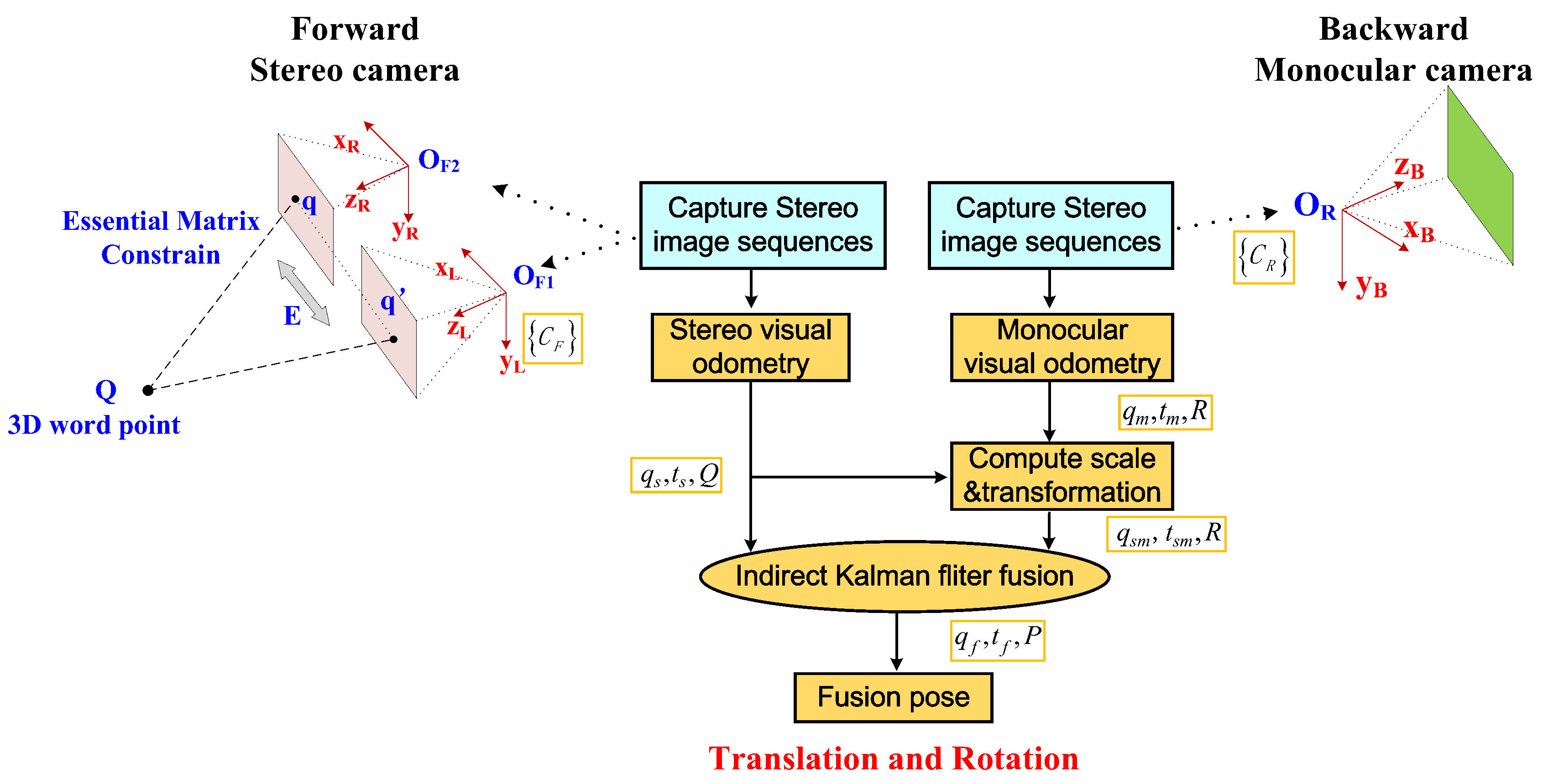
The detail fusion processing of forward stereo camera and backward monocular camera is shown in Figure 3. It shows that our approach runs separate the stereo visual odometry and monocular visual odometry and fusion in the decision level. Therefore, it should be classified to loosely coupled fusion method.

This framework choice would bring several good features. At first, loosely coupled fusion method support the stereo visual odometry and monocular visual odometry working as independent modules, which bring the fusion system with the capability of handing camera module degradation. Second, with the opposite orientation of forward and backward, the fusion pipeline can comprehensively utilize the nearby environment information and take advantage of the time difference from front forward stereo camera to rear backward monocular camera. Third, the system cost is much lower than other construction scheme, such as two sets of stereo vision system, lidar based odometry, or other kinds of precise localization sensor based systems.

2.4. Basic Visual Odometry Method

In our proposed loosely coupled fusion method, featured-based visual odometry was used as the fundamental motion estimation method to compute the translation and rotation of both forward facing stereo camera and backward facing monocular camera and it has a deep influence on the correctness and effectiveness of our method. It has three modules including feature extraction and matching, pose tracking, and local bundle adjustment.

Feature Extraction and Matching: In order to extract and match feature points rapidly, ORB points (Oriented Fast and Rotated BRIEF) were selected as image features, which have good multi-scale and oriented invariance to viewpoints. In the implementation, feature points in each layer of image pyramid space were extracted respectively and the maximum feature points in the unit grid were set to less than five points, making them uniform-distributed. Specifically, for the stereo camera, feature points in the left and right images were extracted simultaneously using two parallel threads and the matching process was employed to delete the isolate points under the epipolar geometry constraints. In the feature matching stage, the Hamming distance was applied to measure the distance of feature points and the best matching should not exceed 30%. Meanwhile, the Fast Library for Approximate Nearest Neighbors (FLANN) method was also used to speed up the feature matching process.

Pose Tracking: The motion model and keyframe based pose tracking method were used to estimate the successive pose of ego vehicle. Firstly, the uniform motion model was used to track feature points and get matching pairs in successive frames with the help of observed 3D map points. With the matching pairs, we can estimate the camera motion using PnP optimization method of minimizing the reprojection errors of all matching point pairs. However, if the matching point pairs are less than certain threshold, the keyframe based pose tracking method woude be activated. Using bag of words(BOW) mode, it can track and match the feature points between the current frame and the closest keyframe.

Local Bundle Adjustment: In this step, the 3D map points observed by closest keyframes were mapped to the current feature points and the poses and 3D map points were adjusted and optimized simultaneously to minimize the reprojection errors. In the application, in order to keep a real-time performance for the system, the maximum number of iterations should be set to a certain value.

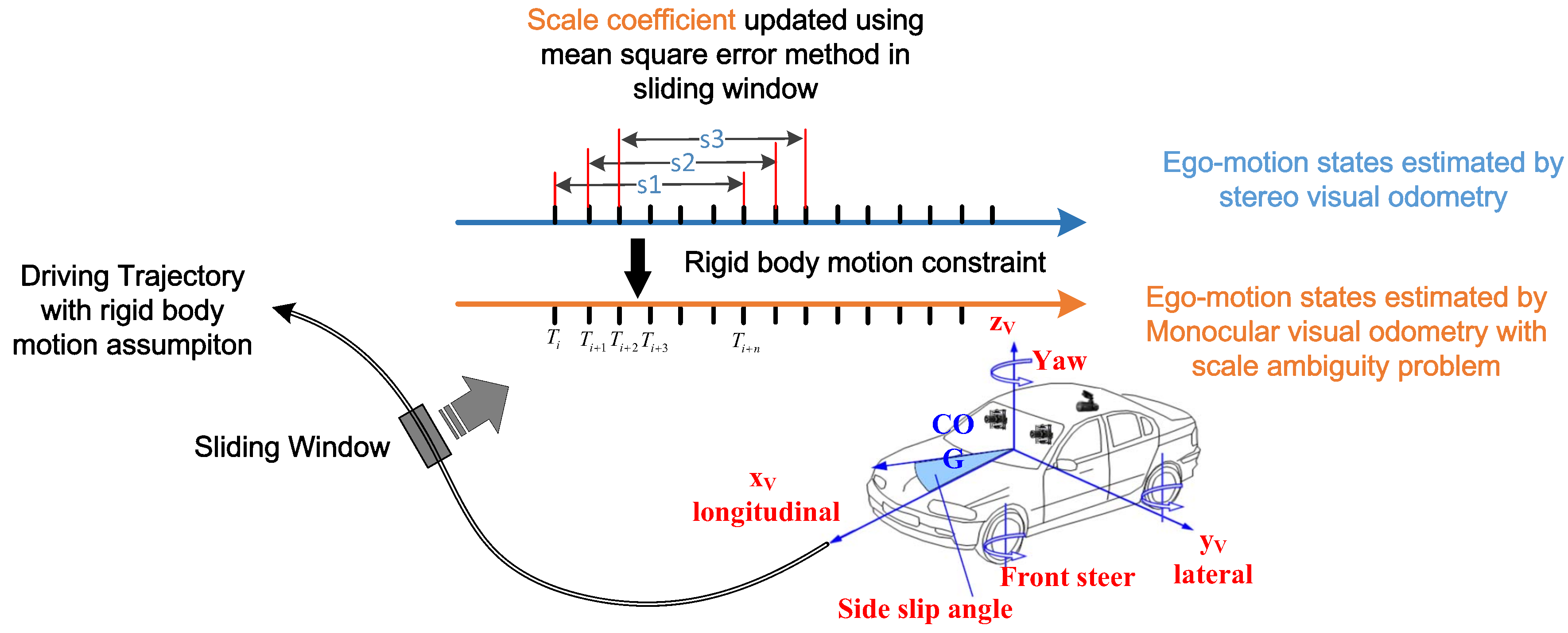
2.5. Scale of Monocular Visual Odometry

To avoid the scale ambiguity in the monocular visual odometry and make it work independently, we use the sliding window based scale estimation method. In the sliding window, mean square error (MSE) was used to dynamically correct and update the scale coefficient under the rigid body motion assumption, as shown in Figure 4.

In the sliding window, we assume that there are n monocular visual odometry states of $t_{m,i},t_{m,i+1},t_{m,i+2}\cdots t_{m,i+n-1}$ and n stereo visual odometry states $t_{sm,i},t_{sm,i+1},t_{sm,i+2}\cdots t_{sm,i+n-1}$. Here, it is noteworthy that, the states of stereo visual odometry has been synchronized to monocular visual odometry states both in spatial and temporal space. Unbiased estimation of the mathematical expectations of those states can be calculated as follows:

$$\overline{t_m}=\frac{1}{n}\sum _i^{i+n-1}{t}_{m,i}\mathrm{and}\overline{t_{sm}}=\frac{1}{n}\sum _i^{i+n-1}{t}_{sm,i}$$

(3)

The above states can be data centralized to $t_{m,i}^{\prime }$ and $t_{sm,i}^{\prime }$ by:

$$t_{m,i}^{\prime }=t_{m,i}-\overline{t_m}\mathrm{and}{t}_{sm,i}^{\prime }=t_{sm,i}-\overline{t_{sm}}$$

(4)

Theoretically, under the rigid body assumption, the relative move distance of the forward stereo camera and backward monocular camera should be equal to each other within the sliding window. So, the problem can be transformed to align the n monocular visual odometry states to the corresponding n points in stereo visual odometry states space.

In practice, there must be some alignment bias and the objective of optimization function should be the minimization of alignment bias. Here, MSE was employed to solve the issue, as in the following equation.

$$\begin{array}{c}min{\displaystyle \sum _i^{i+n-1}}{∥e_i∥}^2=min{\displaystyle \sum _i^{i+n-1}}{∥t_{sm,i}^{\prime }-(sR{t}_{m,i}^{\prime }+r_0^{\prime })∥}^2\hfill \\ =min{\displaystyle \sum _i^{i+n-1}}{∥t_{sm,i}^{\prime }-sR{t}_{m,i}^{\prime }∥}^2-2r_0^{\prime }{\displaystyle \sum _i^{i+n-1}}\left[(t_{sm,i}^{\prime }-sR{t}_{m,i}^{\prime })\right]+n{∥r_0^{\prime }∥}^2\hfill \end{array}$$

(5)

In the equation, $e_i$ is the alignment bias, s is the real scale coefficient of monocular visual odometry, R is the rotation matrix obtained from camera calibration, $r_0^{\prime }$ is the data centralized result of translation value. In order to minimize the alignment bias $e_i$, we can set $r_0^{\prime }$ equal to 0. Then, we get the following equation.

$$\begin{array}{c}min{\displaystyle \sum _i^{i+n-1}}{∥e_i∥}^2=min{\displaystyle \sum _i^{i+n-1}}{∥t_{sm,i}^{\prime }-sR{t}_{m,i}^{\prime }∥}^2\hfill \\ =min({\displaystyle \sum _i^{i+n-1}}{∥t_{sm,i}^{\prime }∥}^2-2s{\displaystyle \sum _i^{i+n-1}}(t_{sm,i}^{\prime }·sR{t}_{m,i}^{\prime })+s^2{\displaystyle \sum _i^{i+n-1}}{∥R{t}_{m,i}^{\prime }∥}^2)\hfill \\ =min({\displaystyle \sum _i^{i+n-1}}{∥t_{sm,i}^{\prime }∥}^2-2s{\displaystyle \sum _i^{i+n-1}}(t_{sm,i}^{\prime }·sR{t}_{m,i}^{\prime })+s^2{\displaystyle \sum _i^{i+n-1}}{∥t_{m,i}^{\prime }∥}^2)\hfill \end{array}$$

(6)

Our goal is to solve the scale coefficient of s and we found that the above equation is a bivariate linear equation, with the following form.

$$\sum _i^{i+n-1}{∥e_i∥}^2=A_{sm}-2sB+s^2{A}_m={(s\sqrt{A_m}-B/\sqrt{A_m})}^2+(A_{sm}{A}_m-B^2)/A_m$$

(7)

with

$$A_{sm}={∥t_{sm,i}^{\prime }∥}^2\mathrm{and}B=\sum _i^{i+n-1}(t_{sm,i}^{\prime }·sR{t}_{m,i}^{\prime })$$

Then, through solving the bivariate linear problem, we can get the result of the scale coefficient of s as:

$$s=\left(\sum _i^{i+n-1}{t}_{sm}^{\prime }·R{t}_m^{\prime }\right)/\sum _i^{i+n-1}{∥t_{m,i}^{\prime }∥}^2$$

(8)

However, in Equation (8), the scale coefficient of s is not symmetric. It means that, there is no reciprocal relation between s (projecting data from monocular visual odometry to stereo visual odometry) and $s^{\prime }$ (projecting data from stereo visual odometry to monocular visual odometry). So, we rewrite the alignment bias $e_i$ into the following form.

$$e_i=\frac{1}{\sqrt{s}}{t}_{sm,i}^{\prime }-\sqrt{s}R{t}_{m,i}^{\prime }$$

(9)

Then, the Equation (7) turns to:

$$\frac{1}{s}{A}_{sm}-2B+s{A}_m={(\sqrt{s}{A}_m-\frac{1}{\sqrt{s}}{A}_{sm})}^2+2(A_m{A}_{sm}-B)$$

(10)

Then, we can get the new result of scale coefficient of $s^{\prime }$ and take it as the scale of current monocular visual odometry sliding window end state $t_{m,i+n-1}$:

$$s^{\prime }=A_{sm}/A_m={(\sum _i^{i+n-1}{∥t_{sm,i}^{\prime }∥}^2/\sum _i^{i+n-1}{∥t_{m,i}^{\prime }∥}^2)}^{1/2}$$

(11)

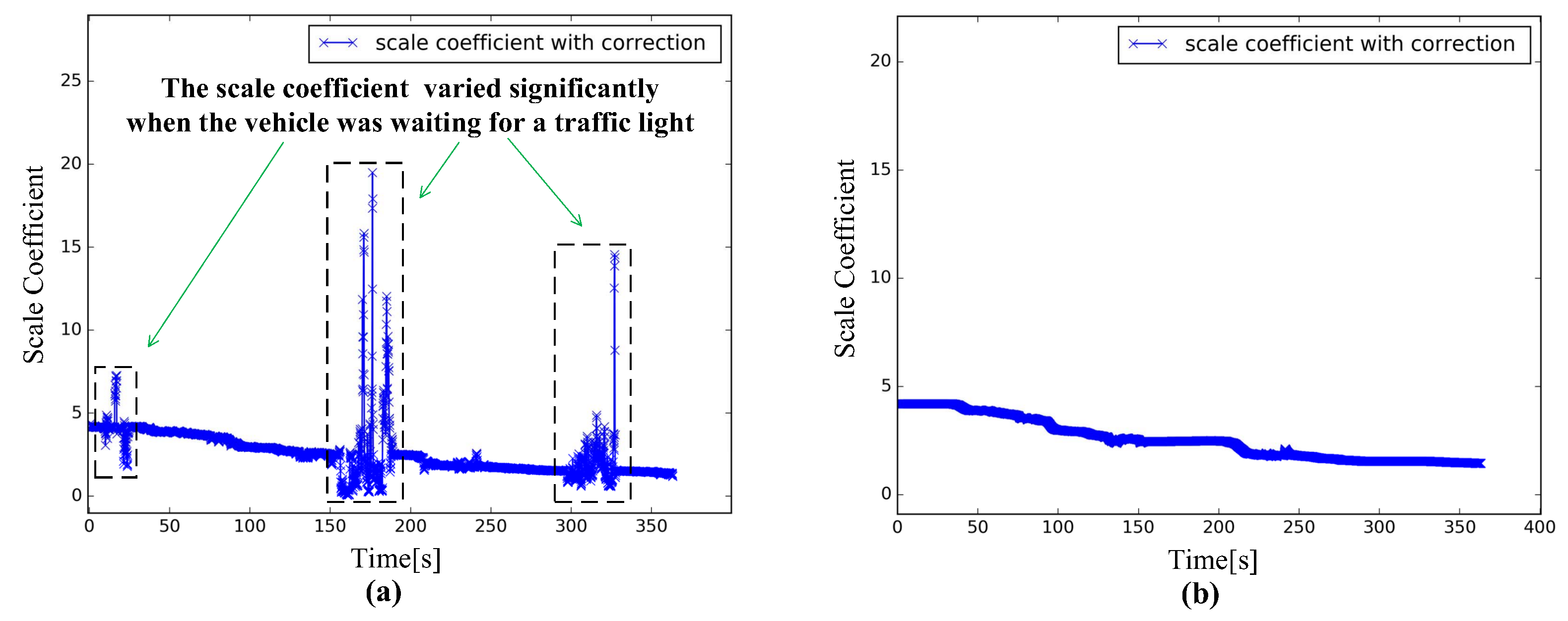
By comparing Formulas (8) and (11), we can know that the new Equation (11) can calculate the scale coefficient $s^{\prime }$ without solving the rotation matrix R. In practice, the scale estimation method is influenced seriously by vehicle motion state, especially stationary state or the changes of motion state. Therefore, we adjust the strategy of scale estimation and correct monocular scale step by step by considering the effect of vehicle motion state.

$$s_{m,i+n-1}^{\ast }=(s_{m,i+n-1}^{\prime }-s_{m,i+n-2}^{\ast })\ast \lambda \ast v{e}_{m,i+n-1}+s_{m,i+n-2}^{\ast }$$

(12)

In this equation, $\lambda$ is the scale updating factor, and $s^{\ast }$ is the updating scale coefficient of monocular visual odometry. The velocity $v{e}_{m,i+n-1}$ is computed in the following steps. At first, computing the initial velocity $v{e}_{m,i+n-1}^{\prime }$ according to aligning stereo visual odometry position based on the uniform velocity model,

$$v{e}_{m,i+n-1}^{\prime }=\frac{\sqrt{{(x_{sm,i+n-1}-x_{sm,i+n-2})}^2+{(y_{sm,i+n-1}-y_{sm,i+n-2})}^2+{(z_{sm,i+n-1}-z_{sm,i+n-2})}^2}}{T_{m,i+n-1}-T_{m,i+n-2}}$$

(13)

Then, we compare the initial velocity $v{e}_{m,i+n-1}^{\prime }$ with the velocity threshold $ve\ast$ (0.04–0.06 m/s in our evaluation) and get the final velocity $ve$,

$$v{e}_{m,i+n-1}=\left\{\begin{array}{ccc}\hfill v{e}_{m,i+n-1}^{\prime },& \hfill & \hfill v{e}_{m,i+n-1}^{\prime }>=ve\ast \\ \hfill 0,& \hfill & \hfill v{e}_{m,i+n-1}^{\prime }<ve\ast \end{array}\right.$$

(14)

Finally, the real value trajectory of monocular visual odometry can be calculated using the updated scale coefficient $s^{\ast }$, as shown in the following equation.

$$t_{am,i+n-1}=R_e\ast s_{m,i+n-1}^{\ast }\ast R_{sm}\ast Rc\ast (t_{m,i+n-1}-t_{m,i})+t_{am,i}$$

(15)

In this equation, $R_e$ is the transformation matrix from forward stereo camere to the backward monocular camera. $R_{sm}$ is the transformation matrix for the different initialization time points. $R_c$ is the transformation matrix from the monocualr coordinate $\left\{C_R\right\}$ to the coordinate $z_B{x}_B{y}_B$ which is opposite to the global coordinate $\left\{G\right\}$ on X-O-Y plane.

2.6. Kalman Filter Based Trajectory Fusion

After giving a dynamically updated scale coefficient to the backward monocular visual odometry, the absolute ego-motion estimation can be correctly obtained. Then, in the sliding window, loosely coupled trajectory fusion was operated to get precise ego-motion estimation, using two-layers Kalman filter method.

2.6.1. Prediction Equation and Observation Equation

In the sliding window $[T_i,T_{\mathrm{i}+n-1}]$, we first take the ego-motion state from forward stereo camera $\Delta x_{(i,i+n-1)s}$ as the state variable and establish state prediction equation as Formula (14). Then, we take the ego-motion state from backward monocular camera $\Delta x_{(i,i+n-1)m}$ as the observation and establish observation equation as Formula (15).

$$X_{(i,i+n-1)}=I\Delta x_{{(i,i+n-1)}_s}+w_{i,i+n-1)}$$

(16)

$$Z_{(i,i+n-1)}=I\Delta x_{{(i,i+n-1)}_m}+v_{(i,i+n-1)}$$

(17)

Here, $w_{(i,i+n-1)}$ is white Gaussian noise of state prediction equation, with covariance matrix of $Q_{(i,i+n-1)}$; $v_{(i,i+n-1)}$ is white Gaussian noise of observation equation, with covariance matrix of $R_{(i,i+n-1)}$. I is an identity matrix.

2.6.2. Calculation of Covariance Matrix

Accurately determining the covariance matrix Q and R would affect the accuracy of the trajectory fusion results. In the proposed method, the matching error of all image frames in the sliding window is considered during the calculation of visual odometry. We use minimum optimization error of each frame to measure the accuracy of the matching confidence and determine the covariance matrix.

Feature points based visual odometry is applied for both forward stereo camera and backward monocular camera and sparse 3-D map points are also reconstructed by different approaches. Here, we use back projection method for stereo camera and use triangulating method for monocular camera. By tracking the feature pairs between sequential images, the ego-motion estimation can be described as a 3D-to-2D problem. In the problem, the RANSAC method is employed to remove outliers. The 3D-to-2D feature pairs from both cameras are all considered in the same optimization function, shown in Equation (16), which tries to minimize the reprojection error of the images and will concern the rigid constraint of the system.

$$\{R,t\}=\underset{R,\mathrm{t}}{argmin}\left(e_{sum}\right)=\underset{R,\mathrm{t}}{argmin}\underset{i\in \chi }{\Sigma }{∥p_i-\pi (R{P}_i+t)∥}_{\Sigma }^2$$

(18)

where, $e_{sum}$ is total reprojection error, R and t are the rotation matrix and translation matrix between successive frames, $\chi$ is the number of inliners of the visual odometry, $i\in \chi$ represent the indexes of feature points in the frame that matching the 3D map points. $p_i$ represent the matched feature points in the frame, $P_i$ are the corresponding 3D points in the 3D sparse map space. $\pi$ is the projection function from 3D to 2D. $\Sigma$ is the total projection error.

From the optimization function Equation (16), we found that the more accuracy of the matching between 3D sparse map points and the corresponding 2D frame point, the better output of the pose obtained by solving the optimization equation. In practice, for the principle of comparability, we take into account of the number of frames in the sliding window and then we can get the mean reprojection error ${\overline{e}}_s$ as:

$${\overline{e}}_{k\in \{s,m\}}=\frac{\eta }{n\ast \chi }\sum _{k\in n}\underset{i\in \chi }{\Sigma }{∥p_i-\pi (R{P}_i+t)∥}_{\Sigma }^2$$

(19)

where $\eta$ is the correction coefficient, n is the number of frames in the sliding window, $k=s$ when it represents stereo visual odometry and $k=m$ for monocular visual odometry. Then, we can use ${\overline{e}}_s$ as diagonal elements to construct the covariance matrix Q for process noise w and can use ${\overline{e}}_m$ as diagonal elements to construct the covariance matrix R for measurement noise v.

2.6.3. Two-Layers Kalman Filter Based Trajectory Fusion

After obtaining the parameters of prediction equation and observation equation, along with the covariance matrix Q and R, we can benefit from the data fusion pipeline. Here, we employed two fusion space for the motion propagation process of both the position estimation and orientation estimation.

In the first level of the fusion stage, the relative position $\Delta t=(\Delta tx,\Delta ty,\Delta tz)$ was estimated in the Euclidean linear space. In the sliding window, the Kalman filter was used to construct the prediction equation and observation equation. The detail was shown in

Table 1. Trajectory obtained by our method in the second experiment.

Steps	Discription	Formula
1	calculate the current predicted value according to the prediction equation	${\tilde{X}}_{(i,i+n-1)}=I\Delta x_{{(i,i+n-1)}_s}$
2	update the covariance matrix of prediction equation	${\tilde{P}}_{(i,i+n-1)}=P_{(i-1,i+n-2)}+Q_{(i,i+n-1)}$
3	calculating kalman gain	$K_{(i,i+n-1)}=P_{(i,i+n-1)}{(P_{(i,i+n-1)}+R_{(i,i+n-1)})}^{-1}$
4	update the predicted value	$X_{(i,i+n-1)}={\tilde{X}}_{i,i+n-1}+K_{(i,i+n-1)}(Z_{(i,i+n-1)}-{\tilde{X}}_{(i,i+n-1)})$
5	update the covariance of the prediction equation	$P_{(i,i+n-1)}=(I-K_{(i,i+n-1)}){\tilde{P}}_{(i,i+n-1)}$

. Where, $\Delta t_{(i,i+n-1)}$ is the estimation of changes of relative position within the sliding window, $t_{f,i}$ and $t_{f,i+n-1}$ are the estimation of ego-motion states. For the Kalman gain $K_{i,i+n-1}$, it is a diagonal matrix and all diagonal elements are same. Hence, we use $k\ast I$ to represent diagonal matrix K and the k is the coefficient of Kalman gain matrix.

In the orientation estimation stage, we proposed an improved Kalman filter, which uses the orientation error space represented by unit quaternion as the state of the filter. In order to construct the motion propagation equation, the state vector of this filter need to be unified with four elements $\Delta q_{(i,i+n-1)}=(qx,qy,qz,qw)$, which can be described as follows:

$$\Delta q_{(i,i+n-1)}=q_{i+n-1}\otimes q_i^{-1}$$

(20)

where, ⊗ represents the multiplication of quaternion.Then, the estimation of orientation propagation states can be acquired by the following equation:

$$q_{f,i+n-1}=\Delta q_{(i,i+n-1)}\otimes q_{f,i}$$

(21)

Here, $\Delta q_{(i,i+n-1)}$ is the estimation of relative orientation changes within the sliding window, $t_{f,i},t_{f,i+n-1}$ are the estimation of ego-motion states represented by the unit quaternion. In this form, the state propagation model and measurement model would be much simpler. Moreover, the processing of the data fusion occurred in the error space was represented by the error quaternion, which could be closer to linear space and, thus, more suitable to the Kalman filter.

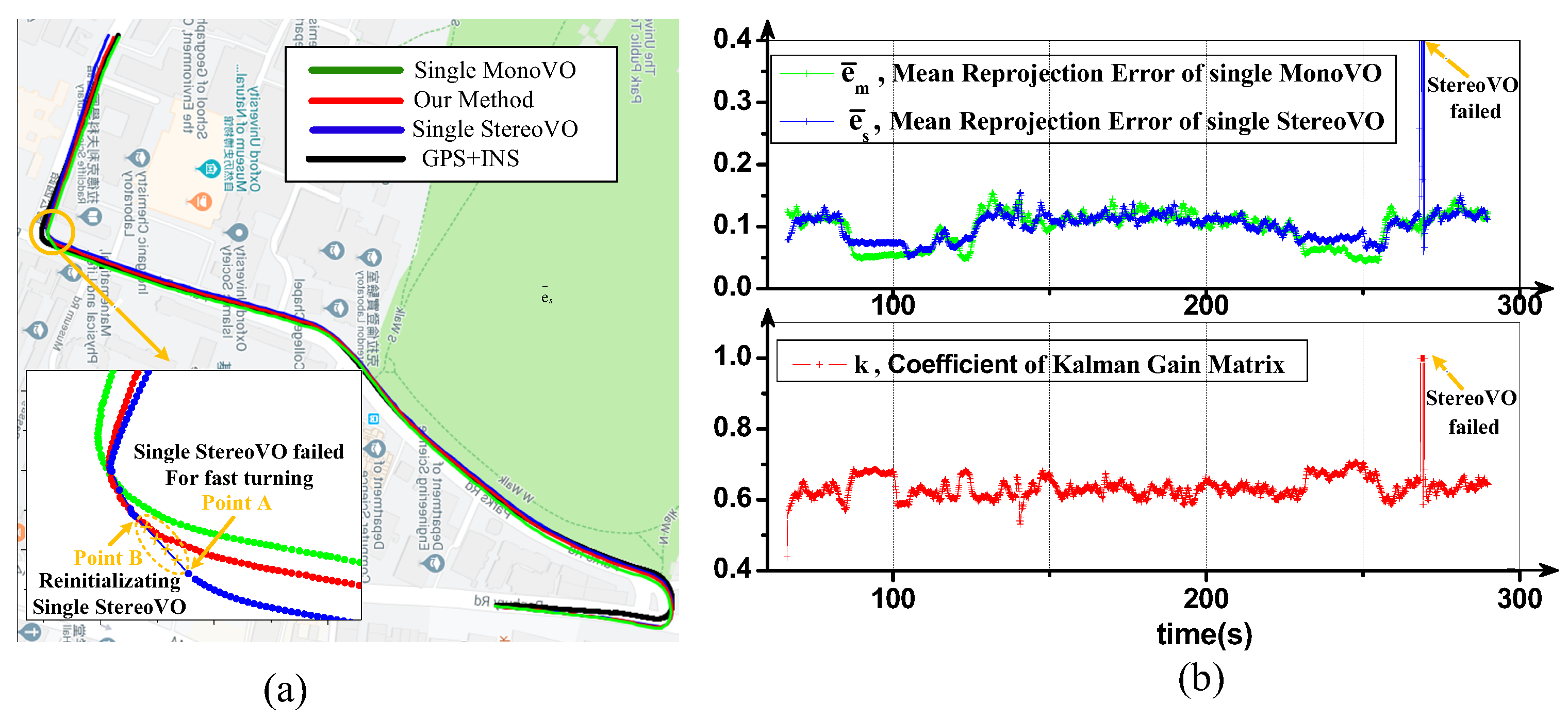
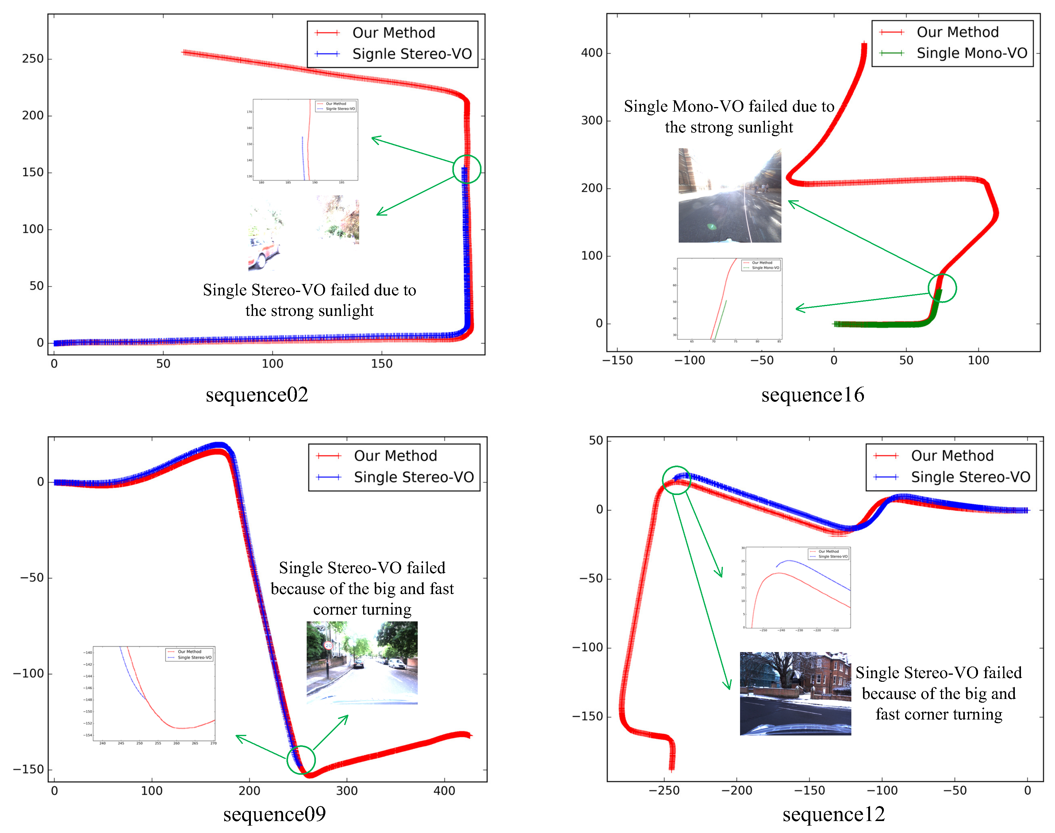
With the proposed trajectory fusion method, the ego-motion states can be computed accurately. When one of the forward-facing stereo camera or backward-facing monocular camera fails, the Kalman filter can automatically update the Kalman gain and reduce the credibility of the impaired camera naturally. It means that the proposed pipeline can fully or partially bypass failure modules and make use of the rest of the pipeline handle sensor degradation.

3. Results

We evaluated the proposed method on the Oxford RobotCar Dataset and compared its performance to some state-of-the-art visual odometry systems. Some key performances, including monocular scale property, robustness capability, and accuracy performance were carried out and comprehensively evaluated.

3.1. Oxford RobotCar Dataset

Oxford RobotCar Dataset [43] was collected by the Mobile Robotics Group, University of Oxford, UK, and it focused on the long-term and large-scale real driving data for autonomous road vehicles, which contains over 1000 km driving data sequences. It was recorded from the car named Nissan LEAF equipping with a Point Grey Bumblebe XB3 trinocular stereo camera, three monocular cameras, three 2D Lidars, GPS and INS.

The reason we chose Oxford RobotCar Dateset as our testing dataset is that it was collected in all weather conditions, including heavy rain, night, direct sunlight and snow, which made it the ideal choice for our evaluation, especially for the robustness and accuracy test. The data in the Oxford RobotCar Dataset are shown in Figure 5.

In our experiment setup, the BumbleeXb3 and the rear Grasshopper2 are selected as the forward and backward cameras in the proposed method. For the trinocular BumbleeXB3, the timestamp of three cameras are synchronized by inherent hardware and the left and right cameras are composed for wider baseline (24 cm) as the forward stereo camera. The relative positioning setup is shown in Figure 6 and the more accuracy calibration extrinsics and camera models are provided in the software development kit (SDK) on their website. In addition, the SDK also supplies us with the Matlab and Python functions for demosaicing and undistorting raw Bayer images.

3.2. Evaluation of Scale Estimation Method

Monocular visual odometry always suffers from the scale ambiguity problem due to the unknown ego-motion translation length between frames. Hence, in this paper, real time scale estimation strategy for backward-facing monocular visual odometry was proposed. In the experiment, we show that the traditional scale estimation method always suffers from the vehicle motion state. For example, Figure 7a depicts that the scale coefficient may vary significantly when the ego-vehicle was waiting for a traffic light and kept still. After considering the effect of vehicle motion state in this paper, the scale coefficient can keep steady and smooth, as shown in Figure 7b.

In order to test the validity of the proposed method, we compared our work with the traditional method proposed by Nist [28], which tends to set the scale of monocular visual odometry to a constant value. As a result, Figure 7 shows that the error caused by the ambiguous scale would continuously accumulated for Nist’s method, which makes the system more prone to deviate from the ground truth. In this paper, the sliding window based scale estimation method was proposed to keep system work stable. In the sliding window, the MSE was used to dynamically correct and update the scale coefficient under the rigid body motion assumption. With this help, In Figure 8, we show that our method can significantly improve the performance of monocular visual odometry.

3.3. Robustness Evaluation

Utilizing the proposed fusion method, the system can fully or partially bypass failure modules and make use of the rest pipeline to handle sensor degradation. Figure 9 demonstrates the fusion procedure and Figure 9 depicts the corresponding fusion confidence. As it shows, with our proposed method, the coefficient of fusion confidence would be updated in real-time according to the matching error of all image frames in the sliding window. Even in the sensor performance degradation point, such as in point A in the following Figures, the system can automatically increase the confidence of the rest undamaged camera naturally to guarantee the safety of the system. In addition, the failed single stereoVO reinitializes successfully at point B.

Further, In order to test the performance of robustness, we compared the proposed fusion method with Single Stereo-VO (single stereo visual odometry) and Single Mono-VO (monocular visual odometry) methods separately. Figure 10 shows that both the Single Stereo-VO and Single Mono-VO may fail under some complicated driving conditions. In sequence 02 of the Oxford RobotCar data set, the Single Stereo-VO failed due to the strong sunlight, which bring insufficient point features for the matching steps. The situation also happened in the sequence 16 for the Single Mono-VO system. In sequence 09 and sequence 12, the Single Stereo-VO lost effectiveness because of the big and fast corner turning. Where, during the quick turning, large motion between corresponding feature points of images would lead to the matching errors and made the system become invalid.

In our proposed system, the data processing pipeline was carefully designed to handle sensor degradation. Some comparative experiments in Figure 10 show that the proposed system has higher robustness than the single stereo and monocular visual odometry. It can still work even under the harsh conditions in which one of the cameras fails.

In order to test the robustness of the system in harsh environments, we also compared the proposed method with some state-of-the-art works including ORB-SLAM2 [33], DSO-Mono (direct sparse monocular odometry) and DSO-Stereo (direct sparse stereo odometry) [44] algorithms using our collected dataset. Our dataset contains 14 sequences of harsh driving environment, such as rain, dusk, night, snow, direct sunlight, texture-less, intense illumination, bumpy road, and fast turns. The performance of the above mentioned works in the dataset is shown in

Table 2. Robustness Peformance Comparison of Different Methods in the Oxford Robotcar Dataset.

	Sequence Description	Duaring Time (s)	Frame Numeber	DSO Mono	DSO Stereo	ORBSLAM2 Stereo	OurMethod Fusion
Seq01	sun, traffic light	224	2485	T	F	F	T
Seq02	strong sunlight	206	2267	F	F	F	T
Seq03	ovrecast, sun	190	2096	T	T	T	T
Seq04	rain, overcast	109	1205	T	F	T	T
Seq05	overcast, traffic light	365	4027	T	F	F	T
Seq06	rain, overcast	151	1665	F	F	T	T
Seq07	dusk, rain	183	2020	T	F	T	T
Seq08	overcast, loop road	224	2474	T	T	F	T
Seq09	sun, clouds	90	2690	F	F	F	T
Seq10	night, dark	163	1795	T	F	T	T
Seq11	snow	119	1314	T	T	T	T
Seq12	snow, traffic light	252	2780	T	T	F	T
Seq13	illumination change	152	1672	T	T	T	T
Seq14	strong sunlight	188	2112	T	F	F	T
Total	–	–	–	11/14	5/14	7/14	14/14

. During the experiment, some methods failed due to strong lighting and some failed in turning corners. In total, the DSO monocular method and DSO stereo method failed 3 times and 9 times respectively, and the ORB-SLAM2 failed 7 times. However, our proposed method always kept a good performance for all the testing sequences.

3.4. Accuracy Evaluation

The accuracy of the proposed method was also evaluated. Firstly, the absolute translation root mean-square error (RMSE) [45] was employed as the quantitative metric to evaluate the performance of accuracy. Sequence 05 in Oxford RobotCar Dataset was used as the testing data, which was captured by forward-facing Bumblebee XB3 stereo camera and the backward-facing Grasshopper2 camera. The GPS + INS (NovAtel) data was used as the ground truth. In the testing dataset, the speed of ego-vehicle changed quickly and encountered a number of red lights. In order to evaluate the performance, some state-of-the-art monocular and stereo visual odometry methods were compared. In the experiment, the trajectories of monocular visual odometry were aligned to the ground truth using the similarity transformation method for the lacking of scale. The results are shown in Figure 11 and

Table 3. Comparison of RMSE of four methods.

Method	Setting	RMSE (m)	RMSE (%)
S-ORBSLAM2	Stereo	6.81	0.519
M-DSO	Monocular	44.22	3.372
M-ORBSLAM2	Monocular	41.90	3.195
Our fusion Method	Multicamera	5.49	0.419

.

From the results we can see that the accuracy of the monocular camera based methods of M-DSO and M-ORBSLAM2 obtained the RMSE of 3.372% and 3.195% respectively, which were poor compared to the stereo camera based methods because the monocular visual odometry always suffered from scale ambiguity problem. In contrast, our method output the best accuracy performance among the 4 state-of-the-art methods [33,44,46] with the RMSE of 0.419%, which is lower than the S-ORBSLAM2 method with the RMSE of 0.519%. This was because our method can take advantage of the outstanding features of symmetry-adaption configuration of forward and backward cameras and comprehensively utilizing the nearby environment information.

In the second experiment, we employed the average error (including AEX, AEY and AED) [47] as the quantitative metric to evaluated the performance of accuracy. Among three average error metrics, the assessment data of AED is more important than the others, since AEX and AEY depend on the choice of the coordinate system, while AED is invariant to it. The calculation equation is shown in the following:

$$\begin{array}{c}AEX=\frac{{\sum }_{i=0}^N\left|X_i-X_i^{GT}\right|}{N}\mathrm{and}AEY=\frac{{\sum }_{i=0}^N\left|Y_i-Y_i^{GT}\right|}{N}\end{array}$$

(22)

$$\begin{array}{c}AED=\frac{{\sum }_{i=0}^N\sqrt{{(X_i-X_i^{GT})}^2+{(Y_i-Y_i^{GT})}^2}}{N}\end{array}$$

(23)

Here, N is the number of frames, $X_i^{GT}$ and $Y_i^{GT}$ are the ground-truth values in X direction and Y direction obtained by the GPS + INS at the $ith$ frame. $Xi$ and $Yi$ are the output results in X direction and Y direction obtained by the corresponding odometry method at the ith frame.

The experiment was carried out in sequence 18 of the Oxford RobotCar Dataset was on a drizzly day. We compared the proposed method with some state-of-the-art algorithms including S-ORBSLAM2 [33] and S-VINS (Stereo Visual-Inertial Systems) [46]. The visual results of the odometry estimations of different methods are shown in Figure 12, which shows the trajectories consisting of each $(Xi,Yi)$ point. The ground-truth trajectories for each $(X_i^{GT},Y_i^{GT})$ point were plotted as black line in Figure 12. The results of the corresponding average error (including AEX, AEY, and AED) are also given in

Table 4. Average Trajectories Errors of Varied Method in the Oxford RobotCar Dataset.

Method	AEX (m)	AEY (m)	AED (m)
S-ORBSLAM2	5.84	12.41	14.30
S-VINS	4.55	12.19	13.89
Our Method	1.83	7.14	7.60

. The results show that our method can achieve the best performance on AED, AEX and AEY among all the methods, which indicates that the output results of our method are the most stable compared with other methods [33,44,46]. In order to clearly demonstrate the results, we mapped the trajectories onto Google earth.

We also present the error curves of all the methods compared with the ground truths from GPS+INS. Figure 13 shows the distance error curve in each frame and the corresponding error for each method. The results show that our proposed method can have smaller overall errors and error boundary compared with other state-of-the-art methods [33,44,46]. So our method is capable of navigating in the real world for kilometers and performs better than other state-of-the-art algorithms.

3.5. Time Results

In this experiment, we tested all sequences 5 times in a computational platform with an Intel Core i5-7500 CPU (four cores @3.4 Hz) and 8 GB RAM to eliminate the randomness in the results. In addition, we set the extracting features as 2000, image pyramid layers as 8 for both stereo and monocular visual odometry systems. The consuming time results of the main modules of our proposed method are shown in

Table 5. Consuming Time Results of Our Proposed Method in Oxford Robotcar Dataset.

Part	Module	Times (ms)
Monocular	Feature Extraction	20.42 ± 4.03
	Pose Tracking	1.54 ± 0.41
	Local Map Tracking	6.02 ± 1.27
	Keyframe Selecting	1.12 ± 0.94
	Total	29.10 ± 6.65
Stereo	Feature Extraction	24.19 ± 3.52
	Stereo Matching	15.73 ± 2.44
	Pose Tracking	2.01 ± 0.34
	Local Map Tracking	8.81 ± 3.12
	Keyframe Selecting	2.72 ± 2.68
	Total	53.46 ± 12.10
Fusion	Scale Computation	0.31 ± 0.12
	KF fusion	0.41 ± 0.17
	Total	0.72 ± 0.29

. Besides, the monocular and stereo visual odometry systems ran at the same time on the distributed robot operating systems. So, the maximum processing frame rate would be decided by the system consuming more time. Therefore, the maximum processing frame rate would be determined by the system that consumes more time. From the table we can see that the total consumption time of our method is about 55 milliseconds with the capability of processing 20 frames per second.

4. Discussion

Based on the obtained results, as well as proving its efficiency, robustness, and accuracy, it can be seen that our approach can achieve superior performance compared with other start-of -the-art methods. The method can fully utilize the information of driving conditions to promote the performance of our positioning system.

Regarding the scale estimation, the scale ambiguity problem of monocular visual odometry has been solved with the MSE optimization method. We show that, in the sliding window, MSE was used to dynamically correct and update the scale coefficient under the rigid body motion assumption. After considering the effect of vehicle motion state, the scale coefficient can keep steady and smooth, which makes the system not easily deviate from the ground truth.

Regarding the robustness, the proposed system can fully or partially bypass failure modules and make use of the rest pipeline to handle sensor degradation. It can still work even under the harsh conditions that one of the cameras fails. The proposed method was also tested in complex driving environments, such as rain, dusk, night, direct sunlight, texture-less, intense illumination, bumpy road, and fast turns. We show that our method can work well in the above mentioned complex and highly dynamic driving environments.

Regarding the accuracy, our method can utilize the remarkable characteristics of symmetry adaption configuration of forward and backward cameras. Meanwhile, a novel fusion mechanism of two-layers Kalman Fusion based data processing framework was employed to comprehensive utilize the nearby environment information. We compare the proposed method with some state-of-the-art works including M-ORBSLAM2, S-ORBSLAM2 [33], M-DSO, S-DSO [44] and S-VINS [46] algorithms. The results show that our method can achieve the best performance on evaluation indexes of AED, AEX, AEY and RMSE among all the methods, which indicates that the output results of our method are most accuracy compared with other methods.

5. Conclusions

We have presented a novel low-cost visual odometry method for estimating egomotion for ground vehicles in challenging environments. To improve the performance of system robustness and accuracy, the scale factor of backward monocular visual odometry was estimated based on the MSE optimization method in a sliding window. Then, in trajectory estimation, an improved two-layers Kalman filter was proposed including orientation fusion and position fusion. The experiments carried out in this paper have proved that our algorithm is superior to other state-of-the-art algorithms.

Different from traditional localization methods that use differential GPS, precise IMU or 3D Lidar, the proposed method only leverages data from inexpensive cameras. Meanwhile, our fusion system employed the outstanding features of symmetry-adaption configuration of forward and backward cameras and provided a new fusion mechanism of two-layers data processing framework to comprehensive utilize the nearby environment information. Therefore, the proposed pipeline can fully or partially bypass failure modules and make use of the rest pipeline to handle sensor degradation making the system more robustness and accuracy.

In future work, we will further optimize our proposed algorithm, reduce its computation complexity, and try to implement it in the compact embedded platform. We will try to integrate other lowcost sensors, such as conventional low-cost GPS, IMU to our system. Meanwhile, we will also explore the method to adjust accelerometer biases using the output of our system, since the velocity measured by our system should be equal to the velocity integrated from the bias-corrected.

References

1. Gluckman, J.; Nayar, S.K. Ego-Motion and Omnidirectional Cameras. In Proceedings of the International Conference on Computer Vision, Bombay, India, 7 January 1998. [Google Scholar]
2. Gabriele, L.; Maria, S.A. Extended Kalman Filter-Based Methods for Pose Estimation Using Visual, Inertial and Magnetic Sensors: Comparative Analysis and Performance Evaluation. Sensors 2013, 13, 1919–1941. [Google Scholar]
3. Wang, K.; Xiong, Z.B. Visual Enhancement Method for Intelligent Vehicle’s Safety Based on Brightness Guide Filtering Algorithm Thinking of The High Tribological and Attenuation Effects. J. Balk. Tribol. Assoc. 2016, 22, 2021–2031. [Google Scholar]
4. Chen, J.L.; Wang, K.; Bao, H.H.; Chen, T. A Design of Cooperative Overtaking Based on Complex Lane Detection and Collision Risk Estimation. IEEE Access. 2019, 87951–87959. [Google Scholar] [CrossRef]
5. Wang, K.; Huang, Z.; Zhong, Z.H. Simultaneous Multi-vehicle Detection and Tracking Framework with Pavement Constraints Based on Machine Learning and Particle Filter Algorithm. Chin. J. Mech. Eng. 2014, 27, 1169–1177. [Google Scholar] [CrossRef]
6. Song, G.; Yin, K.; Zhou, Y.; Cheng, X. A Surveillance Robot with Hopping Capabilities for Home Security. IEEE Trans. Consum. Electron. 2010, 55, 2034–2039. [Google Scholar] [CrossRef]
7. Ciuonzo, D.; Buonanno, A.; D’Urso, M.; Palmieri, F.A.N. Distributed Classification of Multiple Moving Targets with Binary Wireless Sensor Networks. In Proceedings of the International Conference on Information Fusion, Chicago, IL, USA, 5–8 July 2011. [Google Scholar]
8. Kriechbaumer, T.; Blackburn, K.; Breckon, T.P.; Hamilton, O.; Rivas, C.M. Quantitative Evaluation of Stereo Visual Odometry for Autonomous Vessel Localisation in Inland Waterway Sensing Applications. Sensors 2015, 15, 31869–31887. [Google Scholar] [CrossRef] [PubMed] [Green Version]
9. Zhu, J.S.; Li, Q.; Cao, R.; Sun, K.; Liu, T.; Garibaldi, J.M.; Li, Q.Q.; Liu, B.Z.; Qiu, G.P. Indoor Topological Localization Using a Visual Landmark Sequence. Remote Sens. 2019, 11, 73. [Google Scholar] [CrossRef]
10. Perez-Grau, F.J.; Ragel, R.; Caballero, F.; Viguria, A.; Ollero, A. An architecture for robust UAV navigation in GPS-denied areas. J. Field Robot. 2018, 35, 121–145. [Google Scholar] [CrossRef]
11. Yang, G.C.; Chen, Z.J.; Li, Y.; Su, Z.D. Rapid Relocation Method for Mobile Robot Based on Improved ORB-SLAM2 Algorithm. Remote Sens. 2019, 11, 149. [Google Scholar] [CrossRef]
12. Li, Y.; Ruichek, Y. Occupancy Grid Mapping in Urban Environments from a Moving On-Board Stereo-Vision System. Sensors 2014, 14, 10454–10478. [Google Scholar] [CrossRef] [Green Version]
13. Scaramuzza, D.; Fraundorfer, F. Visual Odometry [Tutorial]. Robot. Autom. Mag. IEEE 2011, 18, 80–92. [Google Scholar] [CrossRef]
14. Chen, J.L.; Wang, K.; Xiong, Z.B. Collision probability prediction algorithm for cooperative overtaking based on TTC and conflict probability estimation method. Int. J. Veh. Des. 2018, 77, 195–210. [Google Scholar] [CrossRef]
15. Yang, N.; Wang, R.; Gao, X.; Cremers, D. Challenges in Monocular Visual Odometry: Photometric Calibration, Motion Bias and Rolling Shutter Effect. IEEE Robot. Autom. Lett. 2017, 3, 2878–2885. [Google Scholar] [CrossRef]
16. Mou, X.Z.; Wang, H. Wide-Baseline Stereo-Based Obstacle Mapping for Unmanned Surface Vehicles. Sensors 2018, 18, 1085. [Google Scholar] [CrossRef] [PubMed]
17. Scaramuzza, D. 1-Point-RANSAC Structure from Motion for Vehicle-Mounted Cameras by Exploiting Non-holonomic Constraints. Int. J. Comput. Vis. 2011, 95, 74–85. [Google Scholar] [CrossRef]
18. Zhang, J.; Singh, S. Laser-visual-inertial odometry and mapping with high robustness and low drift. J. Field Robot. 2018, 35, 1242–1264. [Google Scholar] [CrossRef]
19. Siddiqui, R.; Khatibi, S. Robust visual odometry estimation of road vehicle from dominant surfaces for large-scale mapping. IET Intell. Transp. Syst. 2014, 9, 314–322. [Google Scholar] [CrossRef]
20. Ji, Z.; Singh, S. Visual-Lidar Odometry and Mapping: Low-Drift, Robust, and Fast. In Proceedings of the IEEE International Conference on Robotics and Automation, Seattle, WA, USA, 26–30 May 2015. [Google Scholar]
21. Demaeztu, L.; Elordi, U.; Nieto, M.; Barandiaran, J.; Otaegui, O. A temporally consistent grid-based visual odometry framework for multi-core architectures. J. Real Time Image Process. 2015, 10, 759–769. [Google Scholar] [CrossRef]
22. Longuet-Higgins, H.C. A computer algorithm for reconstructing a scene from two projections. Nature 1981, 293, 133–135. [Google Scholar] [CrossRef]
23. Harris, C.G.; Pike, J.M. 3D positional integration from image sequences. Image Vis. Comput. 1988, 6, 87–90. [Google Scholar] [CrossRef] [Green Version]
24. Maimone, M.W.; Cheng, Y.; Matthies, L. Two years of Visual Odometry on the Mars Exploration Rovers. J. Field Robot. 2010, 24, 169–186. [Google Scholar] [CrossRef]
25. Lategahn, H.; Stiller, C. Vision-Only Localization. IEEE Trans. Intell. Transp. Syst. 2014, 15, 1246–1257. [Google Scholar] [CrossRef] [Green Version]
26. Hasberg, C.; Hensel, S.; Stiller, C. Simultaneous Localization and Mapping for Path-Constrained Motion. IEEE Trans. Intell. Transp. Syst. 2012, 13, 541–552. [Google Scholar] [CrossRef]
27. Fraundorfer, F.; Scaramuzza, D. Visual Odometry: Part II: Matching, Robustness, Optimization, and Applications. IEEE Robot. Autom. Mag. 2012, 19, 78–90. [Google Scholar] [CrossRef]
28. Nistér, D.; Naroditsky, O.; Bergen, J.R. Visual odometry for ground vehicle applications. J. Field Robot. 2010, 23, 3–20. [Google Scholar] [CrossRef]
29. Scaramuzza, D.; Fraundorfer, F.; Siegwart, R. Real-Time Monocular Visual Odometry for on-Road Vehicles with 1-Point RANSAC. In Proceedings of the IEEE International Conference on Robotics and Automation, Kobe, Japan, 12–17 May 2009. [Google Scholar]
30. Forster, C.; Carlone, L.; Dellaert, F.; Scaramuzza, D. On-Manifold Preintegration for Real-Time Visual-Inertial Odometry. IEEE Trans. Robot. 2017, 33, 1–21. [Google Scholar] [CrossRef]
31. Pascoe, G.; Maddern, W.; Tanner, M.; Piniés, P.; Newman, P. Nid-Slam: Robust Monocular Slam Using Normalised Information Distance. In Proceedings of the IEEE Conference on Computer Vision and Pattern Recognition, Honolulu, HI, USA, 21–26 July 2017; pp. 1435–1444. [Google Scholar]
32. Nister, D.; Naroditsky, O.; Bergen, J. Visual Odometry. In Proceedings of the IEEE Computer Society Conference on Computer Vision and Pattern Recognition, Washington, DC, USA, 27 June–2 July 2004. [Google Scholar]
33. Mur-Artal, R.; Tardos, J.D. ORB-SLAM2: An Open-Source SLAM System for Monocular, Stereo, and RGB-D Cameras. IEEE Trans. Robot. 2017, 33, 1255–1262. [Google Scholar] [CrossRef]
34. Taylor, C.J.; Kriegman, D.J. Structure and motion from line segments in multiple images. Pattern Anal. Mach. Intell. IEEE Trans. 1995, 17, 1021–1032. [Google Scholar] [CrossRef]
35. Wong, K.Y.K.; Mendonça, P.R.S.; Cipolla, R. Structure and motion estimation from apparent contours under circular motion. Image Vis. Comput. 2002, 20, 441–448. [Google Scholar] [CrossRef] [Green Version]
36. Pradeep, V.; Lim, J. Egomotion Using Assorted Features. In Proceedings of the IEEE Computer Society Conference on Computer Vision and Pattern Recognition, San Francisco, CA, USA, 13–18 June 2010. [Google Scholar]
37. David, N. An efficient solution to the five-point relative pose problem. IEEE Trans. Pattern Anal. Mach. Intell. 2004, 26, 756–770. [Google Scholar]
38. Haralick, B.M.; Lee, C.N.; Ottenberg, K.; Nölle, M. Review and analysis of solutions of the three point perspective pose estimation problem. Int. J. Comput. Vis. 1994, 13, 331–356. [Google Scholar] [CrossRef]
39. Song, Y.; Nuske, S.; Scherer, S. A Multi-Sensor Fusion MAV State Estimation from Long-Range Stereo, IMU, GPS and Barometric Sensors. Sensors 2017, 17, 11. [Google Scholar] [CrossRef] [PubMed]
40. Khan, N.H.; Adnan, A. Ego-motion estimation concepts, algorithms and challenges: An overview. Multimed. Tools Appl. 2017, 76, 16581–16603. [Google Scholar] [CrossRef]
41. Liu, Y.; Chen, Z.; Zheng, W.J.; Wang, H.; Liu, J.G. Monocular Visual-Inertial SLAM: Continuous Preintegration and Reliable Initialization. Sensors 2017, 17, 2613. [Google Scholar] [CrossRef] [PubMed]
42. Zhang, Z. A flexible new technique for camera calibration. IEEE Trans. Pattern Anal. Mach. Intel. 2002, 22, 1330–1334. [Google Scholar] [CrossRef]
43. Maddern, W.; Pascoe, G.; Linegar, C.; Newman, P. 1 year, 1000 km: The Oxford RobotCar dataset. Int. J. Robot. Res. 2017, 36, 3–15. [Google Scholar] [CrossRef]
44. Engel, J.; Koltun, V.; Cremers, D. Direct Sparse Odometry. IEEE Trans. Pattern Anal. Mach. Intell. 2018, 40, 611–625. [Google Scholar] [CrossRef]
45. Sturm, J.; Engelhard, N.; Endres, F.; Burgard, W.; Cremers, D. A Benchmark for the Evaluation of RGB-D SLAM Systems. In Proceedings of the IEEE/RSJ International Conference on Intelligent Robots and Systems, Vilamoura, Portugal, 7–12 October 2012. [Google Scholar]
46. Qin, T.; Pan, J.; Cao, S.; Shen, S. A General Optimization-based Framework for Local Odometry Estimation with Multiple Sensors. arXiv 2019, arXiv:1901.03638v1. [Google Scholar]
47. Yong, L.; Rong, X.; Yue, W.; Hong, H.; Xie, X.; Liu, X.; Zhang, G. Stereo Visual-Inertial Odometry with Multiple Kalman Filters Ensemble. IEEE Trans. Ind. Electron. 2016, 63, 6205–6216. [Google Scholar]
Figure 1. Coordinate system of rigid body motion model with forward stereo camera and backward monocular camera. Using the relative pose transformation matrix, we can transform the trajectories of backward monocular camera into the forward stereo camera Coordinate system. [Color figure can be viewed at www.mdpi.com].
Remotesensing 11 02139 g001
Figure 2. Rigid body motion model based trajectory data synchronization both in spatial and temporal space. [Color figure can be viewed at www.mdpi.com].
Remotesensing 11 02139 g002
Figure 3. Framework of Loosely Coupled Forward and Backward Fusion Visual Odometry. [Color figure can be viewed at www.mdpi.com].
Remotesensing 11 02139 g003
Figure 4. Sliding window based scale estimation of monocular visual odometry. [Color figure can be viewed at www.mdpi.com].
Remotesensing 11 02139 g004
Figure 5. (a) shows the Oxford RobotCar platform with the equipped sensors, and (b) indicates the recording data sequences number in different conditions [43].
Remotesensing 11 02139 g005
Figure 6. The RobotCar platform and sensor positioning setup.The global coordinates and sensor body coordinates are defined.All sensor extrinsics are provided as se(3) format in their software development kit (SDK) tools [43].
Remotesensing 11 02139 g006
Figure 7. (a) shows the result of scale estimation method without considering the effect of vehicle motion state; (b) indicates the better result of our proposed method. [Color figure can be viewed at www.mdpi.com].
Remotesensing 11 02139 g007
Figure 8. The top pictures show the results of Nist’s method with constant scale. By contrast, the bottom pictures shows our method with a better validity and accuracy.
Remotesensing 11 02139 g008
Figure 9. (a) shows that four trajectories, including single MonoVO, single StereoVO, GPS+INS and our method. Single StereoVO fails at point A because of the fast change of scenes and reinitializes at the point B. (b) shows the mean reprojection error ( e ¯ k { s , m } ) of two visual odometry systems and the coefficient of Kalman gain matrix. The failing of Single StereoVO leads to the abrupt change of blue trajectory at the 289 s. For the coefficient k, it is equal to 1, which means that the system only utilizes the information only from single monocular visual odometry.
Remotesensing 11 02139 g009
Figure 10. The top two pictures demonstrate that single stereo visual odometry and single monocular visual odometry sometimes might fail in strong sunlight. The bottom two pictures show they might fail at the corner of fast turning. However, our method always kept a good performance for all the testing sequences.
Remotesensing 11 02139 g010
Figure 11. Trajectory obtained by four methods on sequence 05 in Oxofrd RobotCar Datasets.
Remotesensing 11 02139 g011
Figure 12. Trajectories of 3 methods comparing with the ground truth on the Google earth map. The results show that our proposed method can have smaller overall errors compared with other state-of-the-art methods [33,44,46].
Remotesensing 11 02139 g012
Figure 13. Error curves of varied methods comparing with the ground truth. The horizontal coordinate of the figure was the frame sequences of the camera. The vertical coordinate was the bias value between the ground truth and the estimation in the corresponding frame ( ( X i X i G T ) 2 + ( Y i Y i G T ) 2 ). The curve close to the zero line means the error was small.
Remotesensing 11 02139 g013