Quantifying Tidal Fluctuations in Remote Sensing Infrared SST Observations


Laboratoire d’Océanographie Physique et Spatiale (LOPS), IUEM, Univ. Brest, CNRS, IRD, Ifremer, 29238 Brest, France
*
Author to whom correspondence should be addressed.
†
Current address: Physical & Technological Oceanography Department, Barcelona Expert Center Institut de Ciencies del Mar (ICM), Barcelona, Spain (CSIC).
‡
These authors contributed equally to this work.
Remote Sens. 2019, 11(19), 2313; https://0-doi-org.brum.beds.ac.uk/10.3390/rs11192313
Submission received: 13 September 2019
/
Revised: 2 October 2019
/
Accepted: 3 October 2019
/
Published: 4 October 2019
(This article belongs to the Special Issue Ten Years of Remote Sensing at Barcelona Expert Center)
Abstract
:The expected amplitude of fixed-point sea surface temperature (SST) fluctuations induced by barotropic and baroclinic tidal flows is estimated from tidal current atlases and SST observations. The fluctuations considered are the result of the advection of pre-existing SST fronts by tidal currents. They are thus confined to front locations and exhibit fine-scale spatial structures. The amplitude of these tidally induced SST fluctuations is proportional to the scalar product of SST frontal gradients and tidal currents. Regional and global estimations of these expected amplitudes are presented. We predict barotropic tidal motions produce SST fluctuations that may reach amplitudes of K. Baroclinic (internal) tides produce SST fluctuations that may reach values that are weaker than K. The amplitudes and the detectability of tidally induced fluctuations of SST are discussed in the light of expected SST fluctuations due to other geophysical processes and instrumental (pixel) noise. We conclude that actual observations of tidally induced SST fluctuations are a challenge with present-day observing systems.

1. Introduction
Internal waves (IW) have recently been shown to significantly contribute to sea level variability at scales smaller than about 100 km [1,2,3]. The contamination of IW at theses scales limits our ability to infer ocean currents from altimetric data because IW currents are not related to sea level via geostrophy unlike slower/mesoscale balanced structures [4]. Some IW are of tidal origin and stationary with respect to astronomical forcings, such that the signatures of these waves on altimetric data can be predicted harmonically and eventually removed [5]. Unfortunately most IW are either
- from non tidal origin (e.g., wind-forced, lee-waves).
In both cases, we have no means today to predict these waves.
A direction of research that has been poorly explored yet deals with the signature of IW on satellite data of non-altimetric nature (e.g., sea surface temperature, color) and potential synergies in order to disentangle IW and balanced signatures in altimetric data. We recently proposed in an idealized context a tentative method in order to carry such synergies [8]. While it is premature to apply this method with real data, it may be time to start collecting remote sensing data that: (1) will allow us to verify critical assumptions for such methods (e.g., smallness of IW signature on SST image) and (2) will ultimately be suitable in order to test such methods. The present work is relevant to the former task. We more precisely focus on the quantification of SST fluctuations induced by stationary baroclinic tides because atlases of their distributions are now available [9]. We will also quantify SST fluctuations induced by barotropic tides because the same methodology may be employed for that purpose.
Sea Surface Temperature (SST) is a challenging parameter to define precisely as the upper ocean (within the first 10 m) has complicated vertical variability that is linked to ocean turbulence and air-sea heat fluxes [10]. Methods for determining SST from satellite remote sensing include thermal infrared (IR) and passive microwave radiometry. Both methods have strengths and weaknesses. Thermal IR SST measurements are derived from radiometric observations at wavelengths of ∼3.7 m and/or near 10 m. They provide high spatial resolution SST observations (∼1 to 10 km) and good accuracy (0.1–0.8 K) [11,12], however they are affected by cloud coverage and provide observations only for cloud-free pixels. On the contrary, microwave observations (4–10 GHz) provide a better spatial coverage since they are not affected by cloud coverage but their spatial resolution (∼25 to 50 km) is coarser than IR observations ([13] and references therein). In addition, SST measured from space are representative of a depth that is related to the frequency of the satellite instrument. For example, IR instruments measure a depth of about 20 m, while microwave radiometers measure a depth of a few millimeters [14].
Internal wave modulations of SST from IR aerial observations have been reported at kilometric scales in low-wind conditions [15,16,17,18,19]. Two mechanisms have been considered in order to explain these modulations: fluctuations of the cool-skin temperature (The ocean surface is generally 0.1–0.6 °C cooler than the temperature just below the surface. And this “skin”, or ultra-thin region, is less than a 1mm thick. For further details see http://ghrsst-pp.metoffice.com/pages/documents/DocumentFiles/GDS-v1.0-rev1.5.pdf [last access 8 August 2019]) induced by the internal wave straining field and modulations of the upper diurnal surface layer by vertical displacements of the seasonal thermocline. Internal waves imprint their spatial structure on SST in the aforementioned papers. The present work focuses instead on quantifying of Eulerian, i.e., fixed point, modulations of a pre-existing SST distribution induced by tidal currents and the spatial structure of these modulations is thus not expected to reflect the structure of tidal motions.
This study is based on SST satellite observations, tidal current atlases and an atlas of SST gradients which are described in Section 2. The method to quantify internal wave signature on IR SST observations is explained in Section 3 and results are shown in Section 4. Finally, Section 5 discusses to which extent we may capture SST fluctuations of tidal origin in satellite observations and the main limitations for observing these fluctuations (i.e., pixel noise). All the acronyms used in the manuscript are detailed in the Abbreviation table at the end of the manuscript.
2. Data
2.1. Tidal Current Atlases
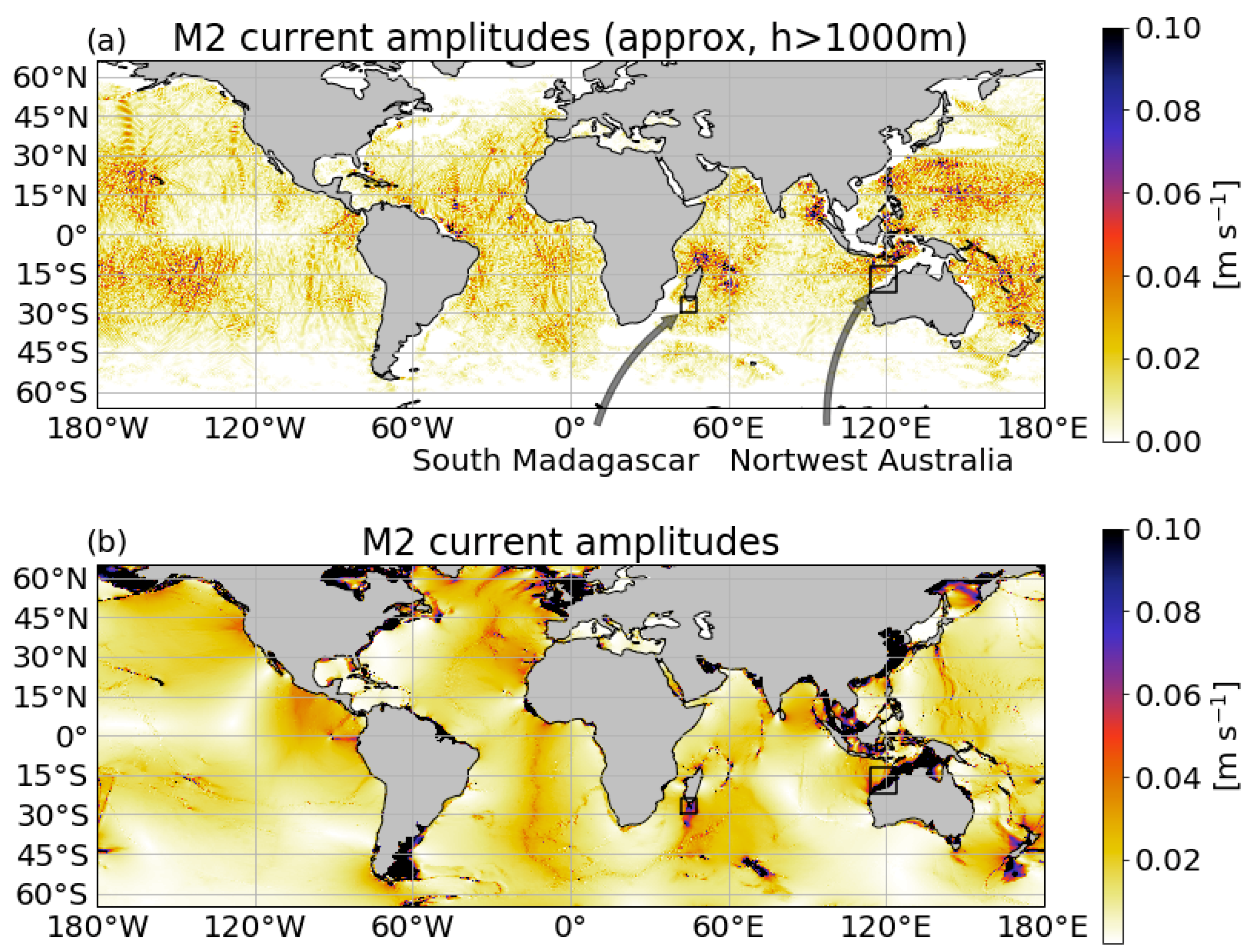
Barotropic tidal currents are extracted from FES2014 which is the current version of the FES (Finite Element Solution) tidal database [20]. Tidal solutions are obtained from an assimilation of tide gauges and altimetric data and delivered on a ° grid. Tidal currents for the M2 constituents are typically of the order to 2–3 cm/s in the open ocean and exhibit a spatial structure characterized by large spatial scales modulated by topography (Figure 1b).
Baroclinic tidal currents are derived from the High Resolution Empirical Tide (HRET) Models [http://web.cecs.pdx.edu/ zaron/pub/HRET.html]. This database has been created to provide baroclinic tide corrections for sea level measurements collected by the upcoming SWOT mission [21]. It was created from an harmonic analysis of sea level anomalies collected by exact repeat altimetric missions (1992–2015). Maps of tidal sea level are provided on a 0.05-degree near-global grid for the 6 most important constituents (M2, S2, K1, O1, N2, and P1 tides). Tidal currents are derived from sea level maps assuming the following momentum equations [9]:
where u, v are zonal and meridional currents, represents sea level, g is gravity, days is damping time scale, and is the tidal frequency. Solutions to (1)–(2) are given by:
where . M2 baroclinic currents exhibit a spatial structure characterized by interfering beams originating from well-defined generation spots (e.g., islands archipelagos, sills) and typical amplitudes around 10 cm/s in the open-ocean (Figure 1a).
2.2. Atlas of SST Gradients
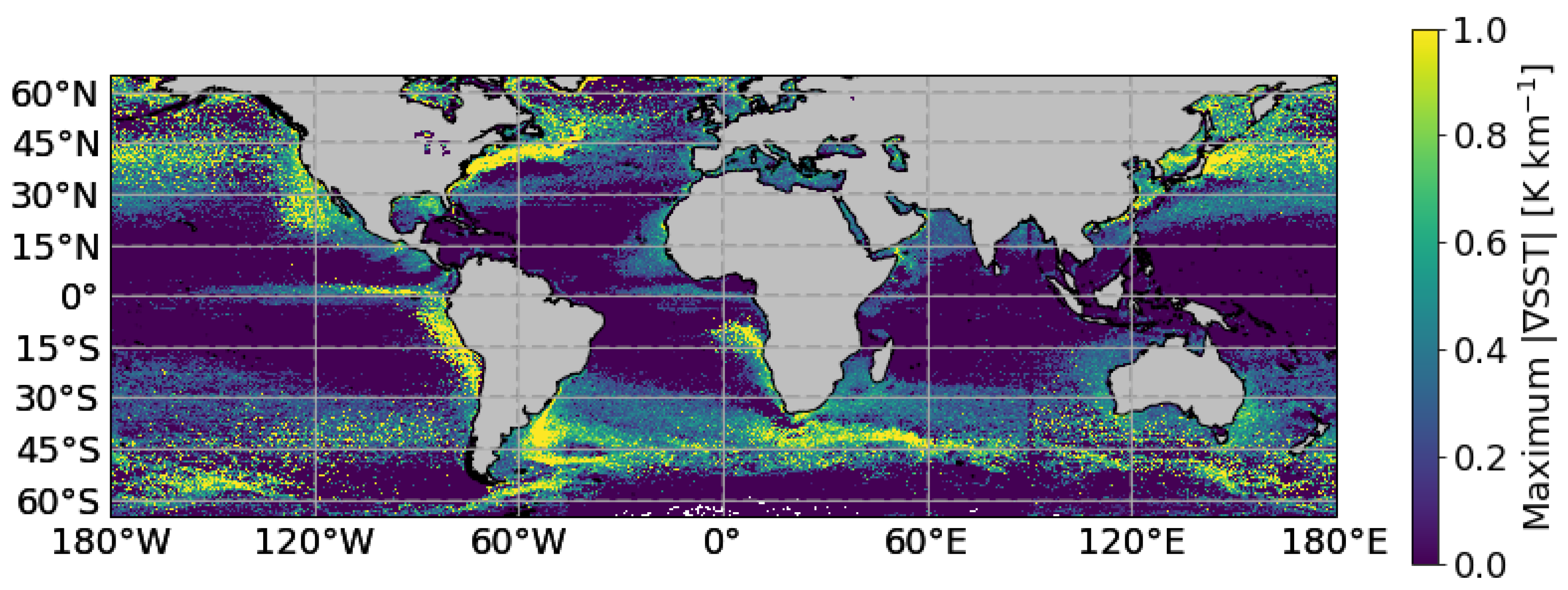
The climatology of the maximum SST gradient magnitude is courtesy of Peter Cornillon, Graduate School of Oceanography, University of Rhode Island (URI). This climatology is obtained from the entire (1985–1996) Pathfinder 9 km resolution SST dataset and is based on the automated procedure by [22] and [23,24,25] and developed by [26,27,28]. Further technical details may be found in this report from the Danish Meteorological Institute (DMI) [29]. The distribution of maximum SST gradient indicates SST spatial gradients exceeding °C near western boundary currents, upwelling areas, the antarctic circumpolar current (Figure 2). The coarser resolution of the SST used for this climatology compared to the SST observations described in Section 2.3 may impact the expected amplitudes of tidally induced SST fluctuations using the climatology. The later may be underestimated compare to what would be estimated with higher resolution SST data to an extent that is difficult to anticipate.
2.3. SST Observations
We use infrared GHRSST SST images captured by several orbiting satellites, particularly, we explored AVHRR-METOP-A (OSISAF) [30], VIIRS and MODIS. In order to find cloud free images, we automatically browsed the entire L2 data catalog for a given region and extracted granules that satisfied a priori selection criteria. The selection procedure consists in dividing the granules in small patches of a fixed size (100 × 100 pixels) and evaluating the ratio of free cloud pixel for each patch individually. To ensure a good spatial coverage, the granule is selected if cloud-free pixel ratio is equal or higher than 80% in at least 30 patches. Finally, the selected granules are remapped onto a regular grid with a spatial resolution of 0.02°. We have explored the L2 data archive from 1 January 2014 to 31 December 2016 for AVHRR-METOP, VIIRS and MODIS.
3. Method
In order to estimate SST fluctuations associated with tidal currents, we assume that tidal motions follow a dynamics that is linear about other motions and adiabatic. Among both assumptions, that of linearity may be occasionally broken for short solitary-type internal waves of tidal origins but is expected valid for open-ocean low-mode internal tides and barotropic tides. Under the aforementioned assumptions, tidal currents transport SST gradients according to:
where is the variation of SST due to tidal currents (w stands for wave), and are the zonal and meridional components of tidal currents, respectively, and stands for the SST. Assuming that:
where , similarly for and , and is the tidal frequency (for M2 constituent rad/s), the amplitude of tidal fluctuations of SST can be estimated as:
The quantification of the SST tidal fluctuations is splitted in three steps:
4. Results
A first attempt at quantifying the expected amplitude of fixed-point SST fluctuations induced by barotropic and baroclinic tidal flows is presented here, by means of two case studies (Section 4.1 and Section 4.2) using infrared SST observations, and at a global scale using clymatological analysis of SST gradients (Section 4.3). The two case studies represent a trade-off between clear sky conditions (see Figure A1) and the intensity of tidal currents (Figure 1).
4.1. Northwest Australia
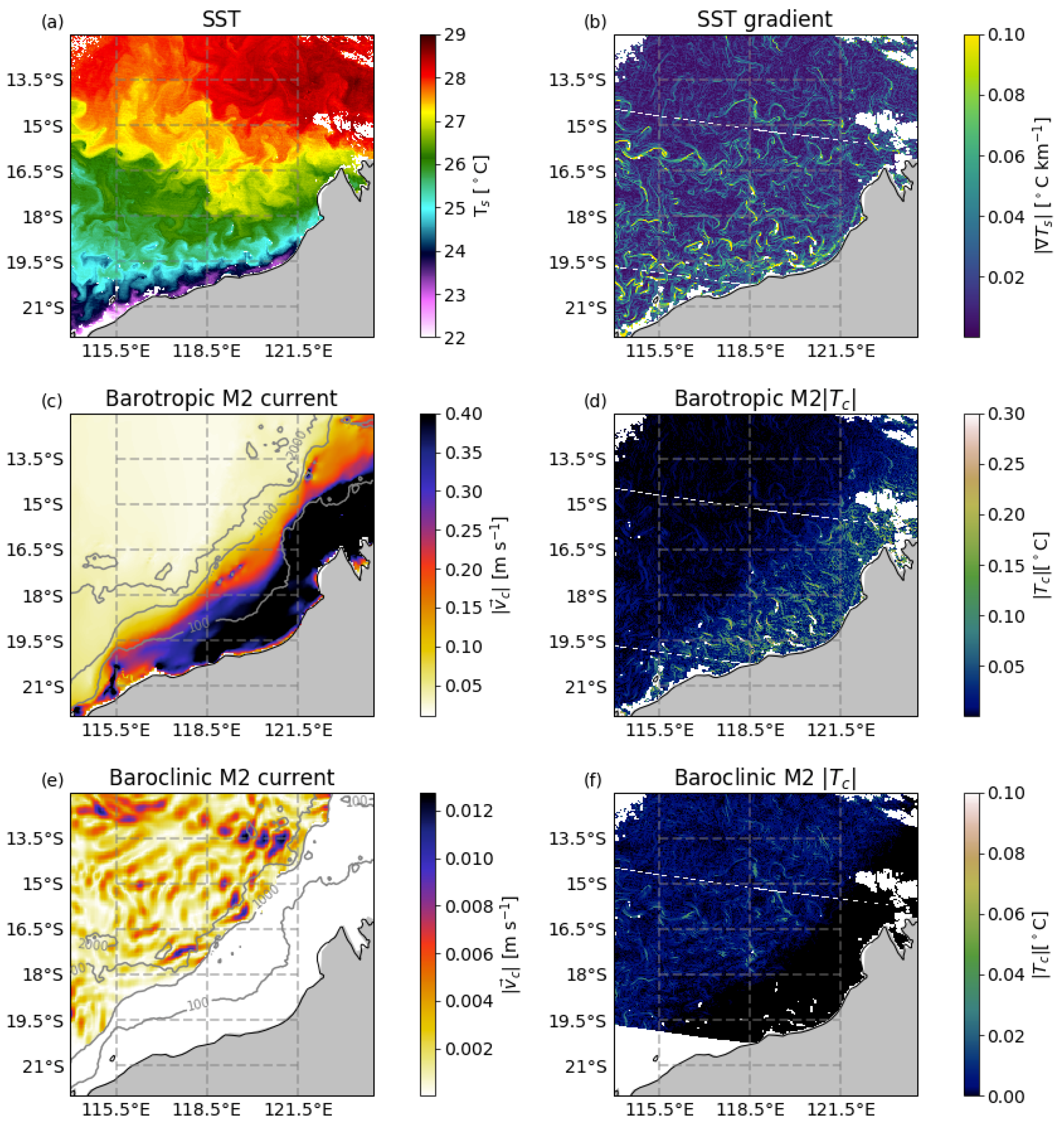
Guided by maps of clear sky probability (Figure A1) and tidal current maps (Figure 1), we focused first on a region located Northwest of Australia, with latitudes between 22°S and 12°S, and longitudes between 114°E and 124°E. We browsed the SST L2 archive (METOP, VIIRS and MODIS) from 2014 to 2016 and selected granules that accomplish at least 30 (100 pixels × 100 pixels) patches with 80% free cloud pixels. Table 1 summarizes the number of available granules for this region. The number of days with more than one L2 granule available is 303 days, which represents a 27% of the analyzed period. The SST corresponding to 8 September 2016 was in particular selected based on this criterium. Gradients of SST were computed and exhibit moderate values around 0.2 °C km.
In this area, semidiurnal internal tide currents (0.08–0.12 m s) are typical of what may be found in the open ocean (Figure 1). These currents are masked over the continental shelf because HRET is not reliable there [9]. Barotropic currents are amplified over the shelf with M2 tidal currents up to 0.6–0.8 m s.
Figure 3 illustrates the procedure to quantify the signature of M2 SST fluctuations for the Northwest Australia case study region. We first compute the Sobel gradient of the SST field then we retrieve M2 baroclinic and barotropic currents for regions. Finally the amplitude of SST fluctuations associated with baroclinic and barotropic currents are estimated by taking the product of SST gradients and tidal currents (Equation (7)).
Both baroclinic and barotropic tidal SST fluctuations are intensified on fronts and filaments. Barotropic fluctuations are largest on the shelf with values up to 0.3 °C and no significant signal in the open ocean (see Figure 3d). Baroclinic SST fluctuations are one order of magnitude smaller, being 0.03–0.04 °C (see Figure 3f).
4.2. South Madagascar
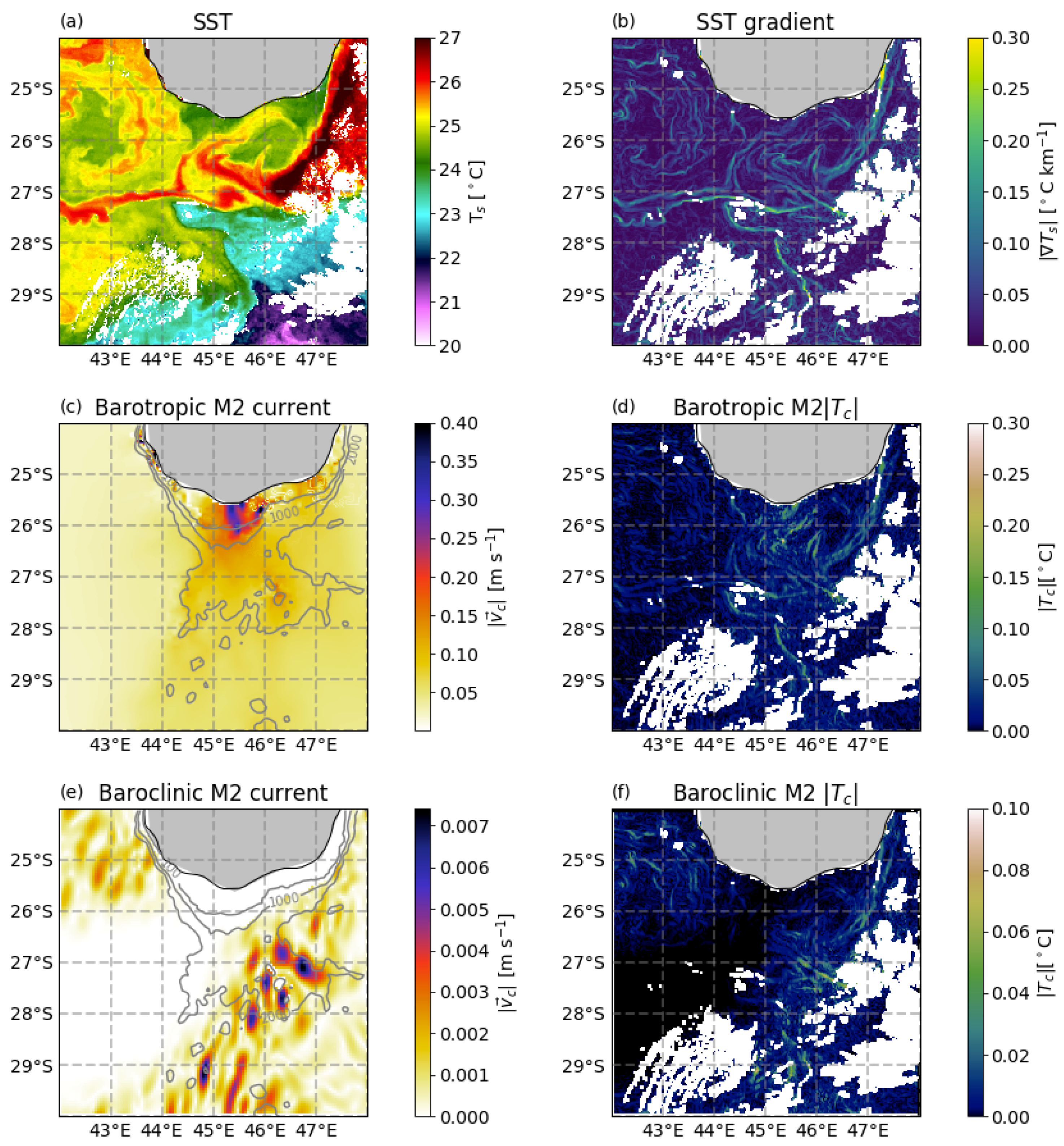
Based again on clear sky maps and tidal currents maps, we selected a second region South of Madagascar (latitude between 30°S and 24°S, longitude between 42°E and 48°E). The number of L2 granules available between 1 January 2014 and 31 December 2016 are summarized in Table 2. For this region, the number of days with more than one granule is 267 (24 % of the period considered). As shown by the METOP SST observation of 5 June 2014 (Figure 4), this region is characterized by strong SST gradients (0.3–0.4 °C km) see Figure 4b).
Both baroclinic and barotropic tidal currents are weaker in this area with values of the order of 0.07 m s and 0.3 m s, respectively. Barotropic currents extend to deep areas, which is different than the Northwest Australia case, shown in Figure 3c.
Figure 4 illustrates the procedure to quantify the signature of the semidiurnal M2 baroclinic motion on SST for the South of Madagascar case study region from a SST image captured by METOP on the 5th June 2014. M2 barotropic currents (see Figure 4c) induce SST fluctuations that are up to 0.2 °C which is less than for the Northwest Australia case. The maximum amplitude of M2 baroclinic tidal SST fluctuations reaches 0.08 °C for this particular case (Figure 4e), i.e., about twice than for the Northwest Australia region. These two opposite trends emphasizes that SST tidal fluctuations result from the product between SST gradients and tidal currents.
4.3. Global Scale
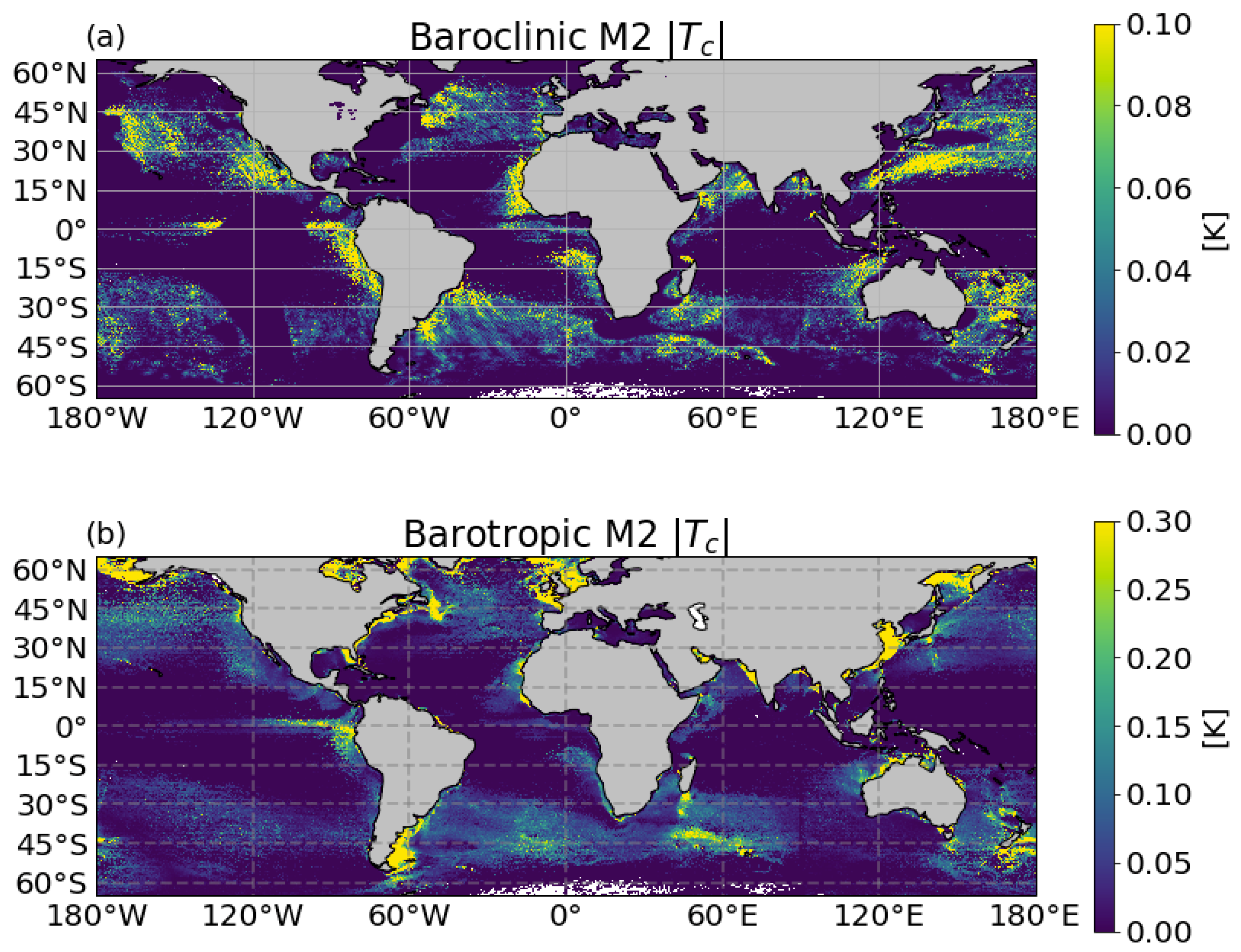
A global perspective on SST tidal fluctuations (Figure 5) is obtained by combining the map of maximum SST gradients (Figure 2) and maps of tidal current amplitudes (Figure 1) as described in Section 3. In this case, since the maximum SST spatial gradient climatology has coarser spatial resolution, it was remapped to onto the grid of the tidal current amplitudes using a bilinear interpolation. Over Northwest Australia and South Madagascar, climatological values of maximum gradients are about °C/km and °C/km respectively, which is between 2 and 6 times more than maximum SST gradients in the two scenes selected (Figure 3 and Figure 4). The same ratio directly reflects into expected tidal SST fluctuation amplitudes.
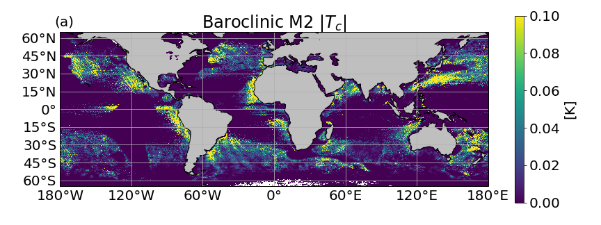
Baroclinic tidal currents cause largest SST fluctuations around western boundary currents main flow paths, except in the case of the Gulf Stream where the baroclinic tidal current is weak or non-existent (see Figure 1), and nearby upwelling areas. The signal is in general weaker for latitudes within ° equatorial areas. When barotropic currents are large, they induce largest SST signals, i.e., in coastal areas, and with a geographical distributions that thus significantly differs from that associated to baroclinic currents. The amplitude of barotropic tidal SST fluctuations is about three times larger than the one induced by baroclinic currents.
5. Discussion and Conclusions
Baroclinic tidal currents derived from the HRET database correspond to the stationary part of the internal tide signal, i.e., fluctuations that keep a fixed phase relationship with astronomical forcings. These currents represent a fraction of actual baroclinic tidal currents [7]. Therefore, present estimates of baroclinic tidal SST fluctuations may underestimate true fluctuations. This is in particular true over western boundary currents paths (see SST fluctuations minima on Figure 5), where the baroclinic tides are non-stationary to a large extent.
For the sake of brevity, this study has focused on one tidal constituent (M2). Constructive interference with other constituents may therefore modulate present estimates of SST tidal fluctuations. The present analysis may be adapted in order to quantify the amplitude of these modulations. It may also be adapted in order to estimate SST fluctuations by other types of fast oceanic motions such as near-inertial waves [33]. Near-inertial currents are for example at least as energetic as baroclinic tidal ones.
Can we hope to capture SST tidal fluctuations in satellite observations? Consecutive observations of SST may allow the identification of propagating SST fluctuations. This identification may be conditioned by the relative importance of SST tidal fluctuations compared to that induced by other geophysical processes (diurnal cycle, mesoscale, submesoscale motions) and noise. SST tidal fluctuations inherits their spatial structures from frontal features, i.e., of the order of kilometers, which is marginally larger than satellite resolutions. These small scale fluctuations will occur coherently over tidal currents spatial scales (Figure 1) nonetheless, and this may be leveraged in order to identify SST tidal fluctuations. The diurnal cycle of SST is expected to have large spatial scales and thus be clearly distinguishable from SST fluctuations induced by tides [34]. Mesoscale and submesoscale fluctuations have comparable spatial structures on the other hand, but are slower and non-propagating which may be leveraged in order to distinguish their contributions to SST fluctuations. The small scale structure of tidal SST fluctuations indicates that pixel noise is the source of noise that may limit the observation of these fluctuations.
We have estimated the noise present in the granules used, assuming it is Gaussian [35]. Given this assumption, the standard deviation of the noise can be estimated using the K-clipping method [36]. This method exploits the dominance of noise at short wavelengths and can be explained as follows. A first guess of is obtained as the standard deviation of a high-pass frequency version of the initial field. Then those values with amplitude higher than K times are rejected, and a new estimation of is obtained from the standard deviation of the remaining values. This is performed iteratively until is obtained, then. In practice three iterations () are enough [36]. The estimated noise standard deviation of the granules considered in the case studies presented in this work is shown in Table 3. It is in general comparable with or smaller than expected SST tidal fluctuations.
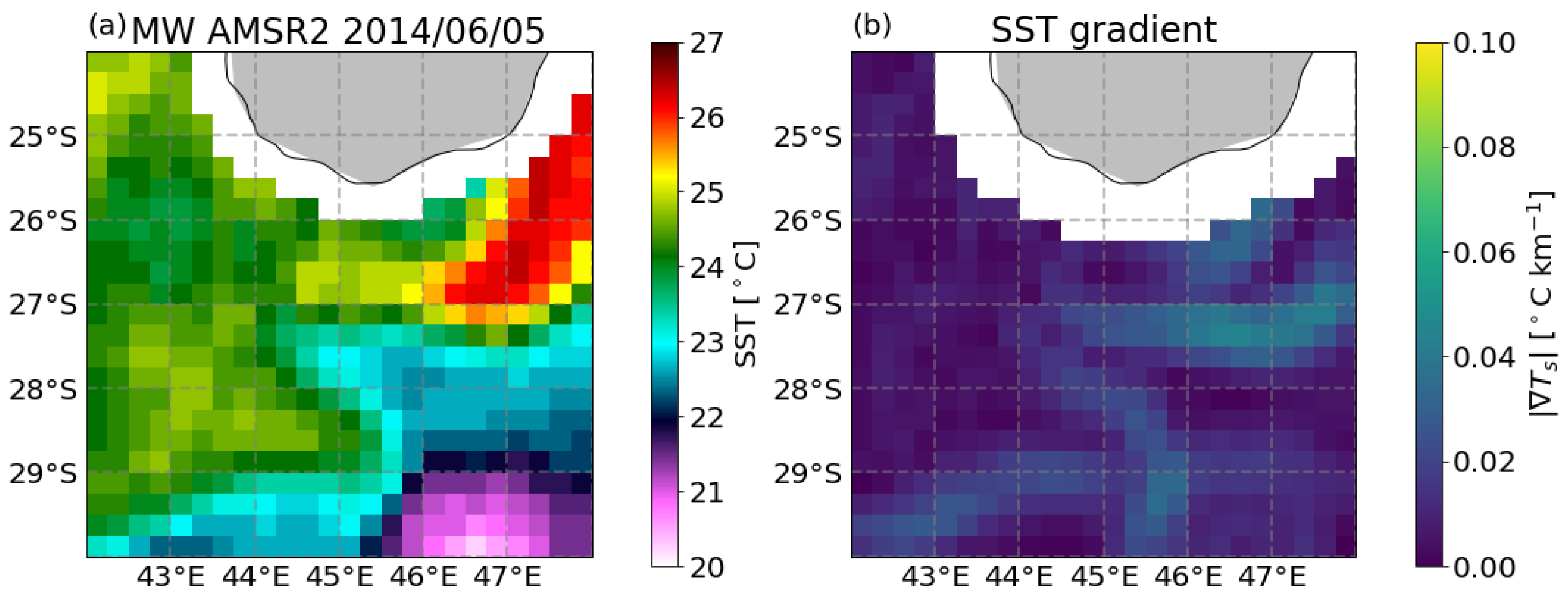
Despite the signature of IW on SST exhibit fine-scale spatial structures and thus IR SST observations are more suitable to quantify tidal fluctuation in SST, we explored whether microwave SST observations could be used to extract low-mode stationary internal tides. Figure A2 shows an example of microwave SST captured by AMSR2 for the same case study shown in Section 4.2. Only stronger gradients of SST are captured and its amplitude is halved compared to the IR SST field shown in Figure 4. Similar results have been already reported by [37] in other regions such as the Gulf Stream or California. Despite these weaker values, the larger amount of available microwave data may be beneficial for the extraction of temporally coherent tidal signals and this should be subject for future work.
The following steps are therefore to search for consecutive snapshots of SST in areas of interest. Infrared geostationary satellites may be useful for this purpose (Himawari, SEVIRI). The global maps in the present paper highlights several regions (on top of the two selected here) where tidal variability is important and cloud density is favorable: Patagonian shelf, west Florida shelf, Moroccan shelf, Persian Gulf, East Indian shelf, Strait of Gibraltar.
Author Contributions
The idea of this study was initially designed by Aurélien Ponte. C.G.-H. did most of the work during her PostDoctoral contract at IFREMER. E.A. developed the software to select L2 SST granules from the entired data catalog. All the authors contributed to formal analysis. The paper was written by C.G.-H. and A.P. E.A. contributed to the writing-review and editing of the paper.
Funding
Aurélien Ponte benefited from funding via the ANR project EQUINOx (ANR-17-CE01-0006-01) and CNES TOSCA project “New dynamical tools for submesoscale characterization in SWOT data”. Cristina González-Haro benefited from funding by CNES.
Acknowledgments
The authors would like to acknowledge Peter Cornillon (University of Rhode Island) and Stéphane Saux Picart (Météo-France) for providing the atlas of maximum gradient of SST, as well as Ed Zaron for providing the HRET internal tide database. The data from the EUMETSAT Satellite Application Facility on Ocean & Sea Ice used in this study are accessible through the SAF’s homepage http://www.osi-saf.org. The MODIS L2P sea surface temperature data are sponsored by NASA. The data from the Naval Oceanographic Office are made available under Multi-sensor Improved Sea Surface Temperature (MISST) project sponsorship by the Office of Naval Research (ONR). The authors want to acknowledge the anonymous reviewers for their valuable and helpful comments.
Conflicts of Interest
The authors declare no conflict of interest. The funders had no role in the design of the study; in the collection, analyses, or interpretation of data; in the writing of the manuscript, or in the decision to publish the results.
Abbreviations
The following abbreviations are used in this manuscript:
| ANR | Agence National de la Recherche |
| AMSR2 | Advanced Microwave Scanning Radiometer 2 |
| AVHRR | Advanced Very High Resolution Radiometer |
| CNES | Centre National d’Études Spatiales |
| CSIC | Consejo Superior de Investigaciones Científicas |
| FES | Finite Element Solution |
| GHRSST | Group for High Resolution Sea Surface Temperature |
| HRET | High Resolution Empirical Tide |
| IFREMER | Institut Français pour l’Exploitation de la Mer |
| IR | Infrared |
| IW | Internal Wave |
| MODIS | MODerate resolution Imaging Spectroradiometer |
| OSISAF | Ocean and Sea Ice Satellite Application Facillity |
| SEVIRI | Spinning Enhanced Visible and InfraRed Imager |
| SST | Sea Surface Temperature |
| SWOT | Surface Water and Ocean Topography |
| VIIRS | Visible Infrared Imaging Radiometer Suite |
Appendix A. Free Cloud Pixel Probability
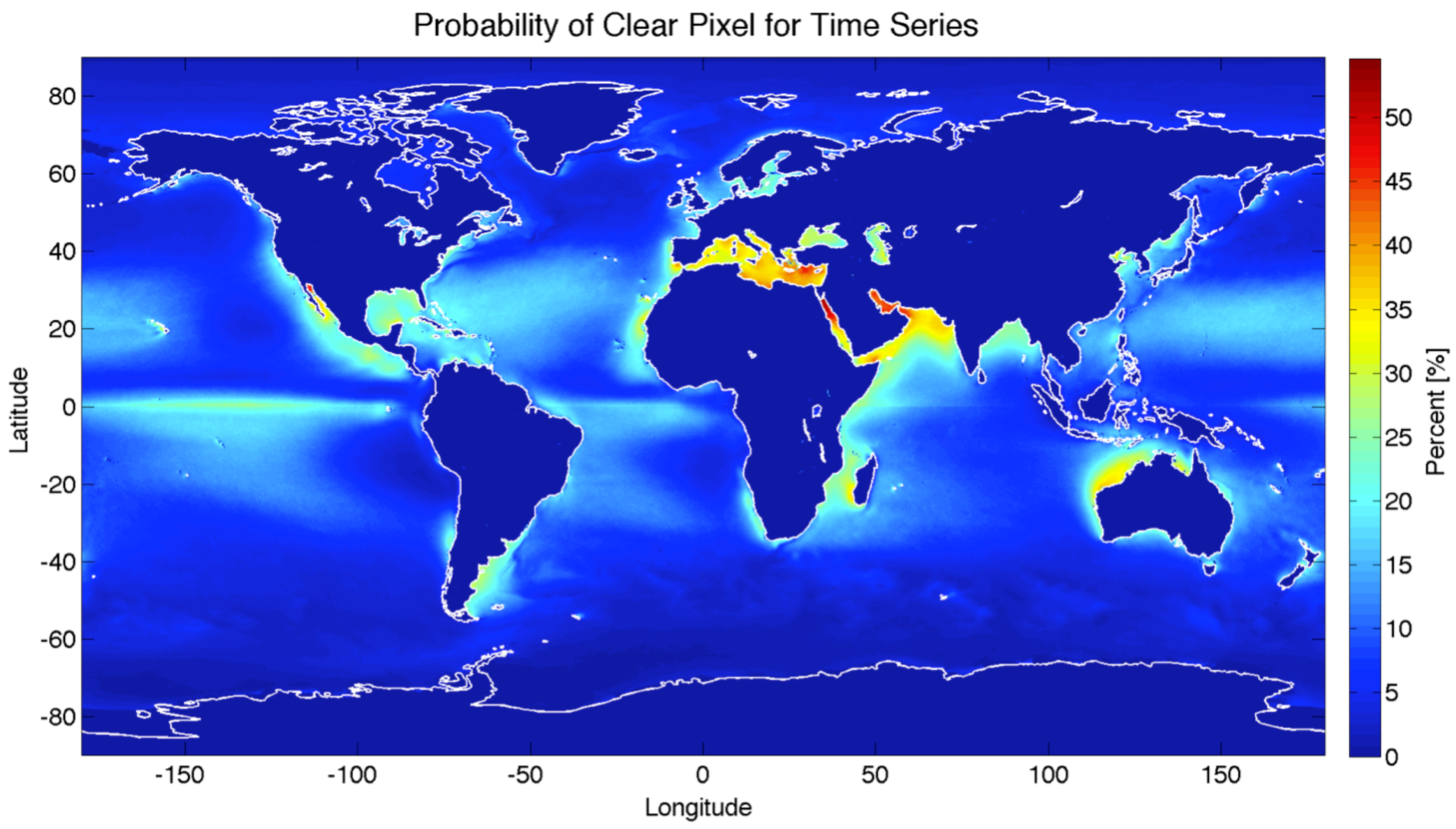
The availability of IR observations is limited by the cloud coverage. Thus, it may be a key parameter to take into account when selecting the regions to study. Figure A1 is included as supporting information to select studied regions.
Figure A1.
Probability of clear pixel for the time series (1982–2011) considered in the climatology of the maximum gradient of SST from University of Rhode Island (URI) Pathfinder 9 km frontal database (courtesy of Peter Cornillon Graduate School of Oceanography, University of Rhode Island (URI)).
Figure A1.
Probability of clear pixel for the time series (1982–2011) considered in the climatology of the maximum gradient of SST from University of Rhode Island (URI) Pathfinder 9 km frontal database (courtesy of Peter Cornillon Graduate School of Oceanography, University of Rhode Island (URI)).

Appendix B. Other SST Observations
Microwave radiometers observations suffer from poor spatial resolution but have great spatial coverage, since they are not affected by the cloud coverage. Their temporal coverage is good for balanced flows but not for IW. We explored to which extent the information about low-modes stationary internal tides (as well as barotropic tides while we’re at it) could be extracted from such data. Figure A2 shows an example of a Microwave SST captured by AMSR2 for the same date than the case study in South Madagascar shown in Section 4.2. As it can be observed by comparing Figure 4 and Figure A2, only stronger gradients can be observed in microwave observations, and its amplitude is reduced by half.
Figure A2.
(a) SST captured by AMSR2 on the 5 June 2014, same date than SST shown in Figure 4 (b) Sobel gradient of SST captured by AMSR2.
Figure A2.
(a) SST captured by AMSR2 on the 5 June 2014, same date than SST shown in Figure 4 (b) Sobel gradient of SST captured by AMSR2.

References
- Richman, J.G.; Arbic, B.K.; Shriver, J.F.; Metzger, E.J. Inferring dynamics from the wavenumber spectra of an eddying global ocean model with embedded tides. J. Geophys. Res. 2012, 117. [Google Scholar] [CrossRef]
- Rocha, C.B.; Gille, S.T.; Chereskin, T.K.; Menemenlis, D. Seasonality of submesoscale dynamics in the Kuroshio Extension. Geophys. Res. Lett. 2016, 43, 11–304. [Google Scholar] [CrossRef]
- Savage, A.C.; Arbic, B.K.; Richman, J.G.; Shriver, J.F.; Alford, M.H.; Buijsman, M.C.; Farrar, J.T.; Sharma, H.; Voet, G.; Wallcraft, A.J.; et al. Frequency content of sea surface height variability from internal gravity waves to mesoscale eddies. J. Geophys. Res. Oceans 2017. [Google Scholar] [CrossRef]
- Arbic, B.K.; Lyard, F.; Ponte, A.; Ray, R.; Richman, J.G.; Shriver, J.F.; Zaron, E.; Zhao, Z. Tides and the SWOT mission: Transition from Science Definition Team to Science Team; Technical Report; CNES: Toulouse, France; NASA: Washington, DC, USA, 2015.
- Ray, R.D.; Zaron, E.D. M2 Internal Tides and Their Observed Wavenumber Spectra from Satellite Altimetry. J. Phys. Oceanogr. 2016, 46, 3–22. [Google Scholar] [CrossRef]
- Ponte, A.L.; Klein, P. Incoherent signature of internal tides on sea level in idealized numerical simulations. Geophys. Res. Lett. 2015, 42. [Google Scholar] [CrossRef]
- Zaron, E.D. Mapping the Non-Stationary Internal Tide with Satellite Altimetry. J. Geophys. Res. Oceans 2016, 122, 539–554. [Google Scholar] [CrossRef]
- Ponte, A.L.; Klein, P.; Dunphy, M.; Gentil, S.L. Low-mode internal tides and balanced dynamics disentanglement in altimetric observations: Synergy with surface density observations. J. Geophys. Res. Oceans 2017. [Google Scholar] [CrossRef]
- Zaron, E.D. Baroclinic Tidal Sea Level from Exact-Repeat Mission Altimetry. J. Phys. Oceanogr. 2019, 49, 193–210. [Google Scholar] [CrossRef]
- Donlon, C.J.; The GHRSST Science Team. The Recommended GHRSST-PP Data Processing Specification; Technical Report v1 revision 1.6; GHRSST: Exeter, UK, 2005.
- Donlon, C.; Rayner, N.; Robinson, I.; Poulter, D.; Casey, K.; Vazquez-Cuervo, J.; Armstrong, E.; Bingham, A.; Arino, O.; Gentemann, C.; et al. The global ocean data assimilation experiment high-resolution sea surface temperature pilot project. Bull. Am. Meteorol. Soc. 2007, 88, 1197–1213. [Google Scholar] [CrossRef]
- Maturi, E.; Harris, A.; Mittaz, J.; Sapper, J.; Wick, G.; Zhu, X.; Dash, P.; Koner, P. A New High-Resolution Sea Surface Temperature Blended Analysis. Bull. Am. Meteorol. Soc. 2017, 98, 1015–1026. [Google Scholar] [CrossRef]
- Hosoda, K. A review of satellite-based microwave observations of sea surface temperatures. J. Oceanogr. 2010, 66, 439–473. [Google Scholar] [CrossRef]
- Donlon, C.; Minnett, P.; Gentemann, C.; Nightingale, T.; Barton, I.; Ward, B.; Murray, M. Toward improved validation of satellite sea surface skin temperature measurements for climate research. J. Clim. 2002, 15, 353–369. [Google Scholar] [CrossRef]
- Walsh, E.J.; Pinkel, R.; Hagan, D.; Weller, R.; Fairall, C.; Rogers, D.; Burns, S.; Baumgartner, M. Coupling of internal waves on the main thermocline to the diurnal surface layer and sea surface temperature during the Tropical Ocean-Global Atmosphere Coupled Ocean-Atmosphere Response Experiment. J. Geophys. Res. Oceans 1998, 103, 12613–12628. [Google Scholar] [CrossRef] [Green Version]
- Marmorino, G.O.; Smith, G.B.; Lindemann, G.J. Infrared imagery of ocean internal waves. Geophys. Res. Lett. 2004, 31. [Google Scholar] [CrossRef]
- Zappa, C.J.; Jessup, A.T. High-Resolution Airborne Infrared Measurements of Ocean Skin Temperature. IEEE Geosci. Remote Sens. Lett. 2005, 2, 146–150. [Google Scholar] [CrossRef]
- Farrar, J.T.; Zappa, C.J.; Weller, R.A.; Jessup, A.T. Sea surface temperature signatures of oceanic internal waves in low winds. J. Geophys. Res. 2007, 112. [Google Scholar] [CrossRef]
- Susanto, R.; Pan, J.; Devlin, A. Tidal Mixing Signatures in the Hong Kong Coastal Waters from Satellite-Derived Sea Surface Temperature. Remote Sens. 2019, 11, 5. [Google Scholar] [CrossRef]
- Carrere, L.; Lyard, F.; Cancet, M.; Guillot, A. FES 2014, a new tidal model on the global ocean with enhanced accuracy in shallow seas and in the Arctic region. In Proceedings of the EGU General Assembly Conference Abstracts, Vienna, Austria, 12–17 April 2015; Volume 17, p. 5481. [Google Scholar]
- Fu, L.L.; Alsdorf, D.; Morrow, R.; Rodriguez, E.; Mognard, N. (Eds.) SWOT: The Surface Water and Ocean Topography Mission; Jet Propulsion Laboratory: Pasadena, CA, USA, 2012.
- Cayula, J.F.; Cornillon, P.; Holyer, R.; Peckinpaugh, S. Comparative study of two recent edge-detection algorithms designed to process sea-surface temperature fields. IEEE Trans. Geosci. Remote Sens. 1991, 29, 175–177. [Google Scholar] [CrossRef] [Green Version]
- Cayula, J.F.; Cornillon, P. Edge Detection Algorithm for SST Images. J. Atmos. Ocean. Technol. 1992, 9, 67–80. [Google Scholar] [CrossRef]
- Cayula, J.F.; Cornillon, P. Multi-Image Edge Detection for SST Images. J. Atmos. Ocean. Technol. 1995, 12, 821. [Google Scholar] [CrossRef]
- Cayula, J.F.; Cornillon, P. Cloud detection from a sequence of SST images. Remote Sens. Environ. 1996, 55, 80–88. [Google Scholar] [CrossRef] [Green Version]
- Ullman, D.S.; Cornillon, P.C. Satellite derived sea surface temperature fronts on the continental shelf off the northeast U.S. coast. J. Geophys. Res. Oceans 1999, 104, 23459–23478. [Google Scholar] [CrossRef]
- Ullman, D.S.; Cornillon, P.C. Evaluation of Front Detection Methods for Satellite-Derived SST Data Using In Situ Observations. J. Atmos. Ocean. Technol. 2000, 17, 1667–1675. [Google Scholar] [CrossRef]
- Ullman, D.S.; Cornillon, P.C. Continental shelf surface thermal fronts in winter off the northeast US coast. Cont. Shelf Res. 2001, 21, 1139–1156. [Google Scholar] [CrossRef]
- Andersen, S.; Belkin, I. Adaptation of Global Frontal Climatologies for Use in the OSISAF Global SST Cloudmasking Scheme; Technical Report 0614; DMI: Bethesda, MA, USA, 2006. [Google Scholar]
- EUMETSAT/OSI-SAF. Low Earth Orbiter Sea Surface Temperature Product User Manual, 3.3 ed.; EUMETSAT: Darmstadt, Germany, 2018. [Google Scholar]
- Sobel, I.; Feldman, G. A 3 × 3 Isotropic Gradient Operator for Image Processing; Stanford Artificial Intelligence Project (SAIL); Stanford University: Stanford, CA, USA, 1968. [Google Scholar]
- Danielsson, P.; Seger, O. Generalized and Separable Sobel Operators. In Machine Vision for Three-Dimensional Scenes; Academic Press: Cambridge, MA, USA, 1990. [Google Scholar]
- Elipot, S.; Lumpkin, R.; Prieto, G. Modification of inertial oscillations by the mesoscale eddy field. J. Geophys. Res. Oceans 2010, 115. [Google Scholar] [CrossRef] [Green Version]
- Kawai, Y.; Wada, A. Diurnal sea surface temperature variation and its impact on the atmosphere and ocean: A review. J. Oceanogr. 2007, 63, 721–744. [Google Scholar] [CrossRef]
- Isern-Fontanet, J.; Hascoët, E. Diagnosis of high-resolution upper ocean dynamics from noisy sea surface temperatures. J. Geophys. Res. Oceans 2014, 119, 121–132. [Google Scholar] [CrossRef]
- Starck, J.L.; Murtagh, F. Astronomical Image and Data Analysis; Springer: Berlin/Heidelberg, Germany, 2006. [Google Scholar]
- Autret, E. Analyse de champs de température de surface de la mer à partir d’observations satellite multi-sources. Ph.D. Thesis, Université Européenne de Bretagne, Rennes, France, 2014. [Google Scholar]
Figure 1.
(a) HRET M2 baroclinic current amplitude for regions with bathymetry(h) deeper than 1000 m (b) FES2014 M2 barotropic current amplitude. The colormap is saturated at 10 cm/s on both figures. Two black boxes delimit the regions of the case study presented in Section 4.1 and Section 4.2, respectively.

Figure 2.
Maximum of the annual climatology of the maximum spatial gradient of SST from University of Rhode Island (URI) Pathfinder 9 km frontal database.
Figure 2.
Maximum of the annual climatology of the maximum spatial gradient of SST from University of Rhode Island (URI) Pathfinder 9 km frontal database.

Figure 3.
(a) SST captured by VIIRS on the 8 September 2016. (b) Sobel gradient of SST. Note that the SST field shown here is composed of three L2 granules. The gradient is computed for each granule individually. Thus, the representation of the gradient presents two scan lines with missing data that correspond to the boundaries of the granules. (c) M2 barotropic FES amplitude current. Gray contour correspond to the bathymetry. (d) Estimation of the amplitude of M2 signature on SST. (e) M2 baroclinic HRET amplitude current for areas with a bathymetry deeper than 1000m. Gray contour lines correspond to the bathymetry. (f) Estimation of the amplitude of M2 IW signature on SST.

Figure 4.
(a) SST captured by METOP on the 5 June 2014. (b) Sobel gradient of SST. (c) M2 barotropic FES amplitude current. Gray contour correspond to the bathymetry. (d) Estimation of the amplitude of M2 barotropic signature on SST. (e) M2 baroclinic HRET amplitude current for areas with a bathymetry deeper than 1000m. Gray contour lines correspond to the bathymetry. (f) Estimation of the amplitude of M2 IW signature on SST.

Figure 5.
(a) Estimation of the amplitude of M2 IW signature on SST. (b) Estimation of the amplitude of M2 barotropic signature on SST.
Figure 5.
(a) Estimation of the amplitude of M2 IW signature on SST. (b) Estimation of the amplitude of M2 barotropic signature on SST.


Table 1.
Number of L2 granules available from 1 January 2014 to 31 December 2016 in the Northwest Australia case study region.
Table 1.
Number of L2 granules available from 1 January 2014 to 31 December 2016 in the Northwest Australia case study region.
| Number of Available L2 Granules | ||||
|---|---|---|---|---|
| 2014 | 2015 | 2016 | TOTAL | |
| METOP | 181 | 124 | 185 | 490 |
| VIIRS | 160 | 147 | 120 | 427 |
| MODIS | 59 | 152 | 120 | 331 |
Table 2.
Number of L2 granules available from 1 January 2014 to 31 December 2016 in the Madagascar case study region.
Table 2.
Number of L2 granules available from 1 January 2014 to 31 December 2016 in the Madagascar case study region.
| Number of Available L2 Granules | ||||
|---|---|---|---|---|
| 2014 | 2015 | 2016 | TOTAL | |
| METOP | 130 | 147 | 114 | 391 |
| VIIRS | 70 | 133 | 145 | 348 |
| MODIS | 143 | 111 | 40 | 249 |
Table 3.
Noise standard deviation of the SST images considered.
| Granule ID | Sensor | Region | (K) |
|---|---|---|---|
| 20160908174014 | VIIRS | Northwest Australia | 0.03 |
| 20160908174139 | VIIRS | Northwest Australia | 0.03 |
| 20160908174305 | VIIRS | Northwest Australia | 1.68 |
| 20140605062503 | AVHRR | South Madagascar | 0.67 |
| 20140605184903 | AVHRR | South Madagascar | 0.06 |
© 2019 by the authors. Licensee MDPI, Basel, Switzerland. This article is an open access article distributed under the terms and conditions of the Creative Commons Attribution (CC BY) license (http://creativecommons.org/licenses/by/4.0/).
Share and Cite
MDPI and ACS Style
González-Haro, C.; Ponte, A.; Autret, E. Quantifying Tidal Fluctuations in Remote Sensing Infrared SST Observations. Remote Sens. 2019, 11, 2313. https://0-doi-org.brum.beds.ac.uk/10.3390/rs11192313
AMA Style
González-Haro C, Ponte A, Autret E. Quantifying Tidal Fluctuations in Remote Sensing Infrared SST Observations. Remote Sensing. 2019; 11(19):2313. https://0-doi-org.brum.beds.ac.uk/10.3390/rs11192313
Chicago/Turabian StyleGonzález-Haro, Cristina, Aurélien Ponte, and Emmanuelle Autret. 2019. "Quantifying Tidal Fluctuations in Remote Sensing Infrared SST Observations" Remote Sensing 11, no. 19: 2313. https://0-doi-org.brum.beds.ac.uk/10.3390/rs11192313
Note that from the first issue of 2016, this journal uses article numbers instead of page numbers. See further details here.