Assimilation of Satellite Salinity for Modelling the Congo River Plume


Space and Atmospheric Physics Group, Department of Physics, Imperial College London, London SW7 2AZ, UK
*
Author to whom correspondence should be addressed.
Remote Sens. 2020, 12(1), 11; https://0-doi-org.brum.beds.ac.uk/10.3390/rs12010011
Submission received: 13 November 2019
/
Revised: 5 December 2019
/
Accepted: 15 December 2019
/
Published: 18 December 2019
(This article belongs to the Special Issue Ten Years of Remote Sensing at Barcelona Expert Center)
Abstract
:Satellite salinity data from the Soil Moisture and Ocean Salinity (SMOS) mission was recently enhanced, increasing the spatial extent near the coast that eluded earlier versions. In a pilot attempt we assimilate this data into a coastal ocean model (ROMS) using variational assimilation and, for the first time, investigate the impact on the simulation of a major river plume (the Congo River). Four experiments were undertaken consisting of a control (without data assimilation) and the assimilation of either sea surface height (SSH), SMOS and the combination of both, SMOS SSH. Several metrics specific to the plume were utilised, including the area of the plume, distance to the centre of mass, orientation and average salinity. The assimilation of SMOS and combined SMOS SSH consistently produced the best results in the plume analysis. Argo float salinity profiles provided independent verification of the forecast. The SMOS or SMOS SSH forecast produced the closest agreement for Argo profiles over the whole domain (outside and inside the plume) for three of four months analysed, improving over the control and a persistence baseline. The number of samples of Argo floats determined to be inside the plume were limited. Nevertheless, for the limited plume-detected floats the largest improvements were found for the SMOS or SMOS SSH forecast for two of the four months.
Keywords:
SMOS; data assimilation; 4D-Var; Congo River plume; satellite salinity; Angola Basin; ROMS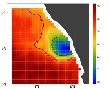
1. Introduction
The ten largest rivers transport a combined 40% of the freshwater and particulate material into the oceans [1,2,3,4]. Some larger rivers can generate offshore plumes of significant distance [4,5] that can support high levels of biological productivity, due to the vast amount of supplied nutrients [6,7]. Therefore, the accuracy of modelling these river plumes is valuable for fishing communities. Furthermore, terrestrial material, both suspended and dissolved, are transported via river plumes, affecting sediment and pollutant distributions and the biogeochemistry of carbon [3].
The second-largest river (in terms of the annual mean daily discharge) is the Congo in West Africa, discharging an average 39,866 m/s of freshwater per month into the Angola Basin. Such extensive outflow produces a plume as large as 800 km from the river mouth [4,5], influencing a substantial section of the basin. Yankovsky and Chapman [8] noted that the plume could be classified as surface-advected; with identifiable near-and far-field regions. Variations in the near-field have been identified with the speed of outflow, the orientation of the estuary mouth and local coastal currents [9,10]. For the far-field, a more complex situation arises through the interaction between the wind stress, ocean circulation patterns, tidal currents and river discharge variations that contribute to different scenarios of the Congo River plume dispersion [11]. Denamiel et al. [10] performed the first numerical simulation of the Congo River plume where they found the plume had a northward extension for the majority of the year except during February-March where the plume had a sizeable westward expansion (up to 800 km). Subsequent model studies have focused on the plume’s buoyancy-driven dynamics [12,13], the effect of the Congo on ocean temperatures [14] and a complete simulation of the Congo river-to-sea continuum with a multi-scale unstructured mesh model [15].
Very few studies have focused on improving forecasting river plumes. Liu et al. [16] produced a realistic hind-cast of the Columbia River estuarine-plume-shelf circulation and used a skill score to quantify the five dynamical regions (estuary, near- and far-field plume, near-surface and deep layers). Data assimilation (DA) is a powerful tool that produces an optimal estimate of the initial conditions (typically for a forecast) using observations and information from the dynamical model [17]. Until recently, DA could not easily be utilised in the context of river plume modelling. While the more traditional Argo floats provide relatively accurate in-situ salinity profiles, their lack of spatial coverage (typically 3 by 3) is a significant limitation. In 2009 the European Space Agency (ESA) launched the first satellite to monitor surface sea salinity under the Soil-Moisture-Ocean Salinity (SMOS) mission [18] providing global coverage of surface salinity. Köhl et al. [19] assimilated SMOS but found no benefits to the global model salinity. Conversely, Lu et al. [18] found that SMOS data plays a complementary role in model salinity simulations with an Ensemble Optimal Interpolation DA scheme (EnOI). A new version of SMOS that dramatically improved the land/sea interference and coastal coverage has been available from 2017 [20]. The Congo River plume can now be fully analysed on a 9-daily scale instead of monthly, expanding the scope of the data for use in coastal assimilation (Figure 1).
A recent study by Mu et al. [21] was the first to show that the assimilation of this newer data could improve simulations of the upper ocean salinity. However, prior to the assimilation, Mu et al. [21] applied an additional bias correction, specific to their study region (South China Sea) using a Generalised Regression Neural Network (GRNN). The assimilation of this bias-corrected GRNN SMOS data set improved results compared to the original data set without such bias correction.
In this paper, the SMOS data as originally produced by Olmedo et al. [20] is assimilated to study the impact on the simulation of the Congo River plume. This will be the first time that satellite salinity has been used with DA specifically for river plumes and the first time a Congo River plume forecast has been attempted. Satellite altimetry sea surface height (SSH) is also assimilated individually and in combination with SMOS, to explore whether these two data streams could compliment each other. The rest of this paper is structured as follows: the materials and method sections introduces the numerical model, observations, assimilation scheme and experiment design. The results then follows split into an assessment of the assimilation analysis and forecast. The paper closes with a discussion on the results and a final conclusion.
2. Materials and Methods
2.1. Numerical Model
ROMS is a hydrostatic, primitive equation, Boussinesq ocean general circulation model [22]. Previous studies have utilised various versions of this ROMS model of the Angola Basin in understanding the Congo River plume dynamics [10], effects on ocean temperature [14] and more recently on the impact of DA on the ocean current predictability [23]. The model domain extends between 1 S–21 S and 3.7 E–13.8 E with a 10 km resolution and 40 terrain-following vertical levels. Lateral boundary and initial conditions for temperature, salinity, ocean current velocities and sea surface height were obtained from the HYCOM reanalysis [24]. Atmospheric forcing at the surface for downward radiative surface fluxes, sea level pressure, 2 m specific humidity, 2 m air temperature, 10 m winds, and total precipitation were obtained from European Centre for Medium-Range Weather Forecasts (ECMWF) reanalysis (ERA)-Interim reanalysis data (ERA-I) [25].
Seven rivers (Nyanga, Kouilou, Kwanza (Cuanza), Kuene, and the Congo) are incorporated into ROMS as boundary conditions. For each river channel, several source points are assigned a unique outflow rate with a constant temperature (15 degrees) and near-zero salinity (0.1 PSU). Following White and Toumi [14], river flow rates were obtained from various sources, including the RivDIS v1.1 database [26], the Global Environmental Monitoring System/Global River Inputs (GEMS/GLORI) database [27], The Office of Industrial Studies Renewable Energies and Environment (BEI ERE) and the University of Brazzaville available at (http://hmf.enseeiht.fr/travaux/CD0809/bei/beiere/groupe5/node/53). The Congo represents the largest of the rivers in the model domain with a channel of 20 km (width) × 60 km (length) (2 × 6 grid points) containing eight source points. The average annual cycle of the Congo River discharge computed from the observed monthly mean between 1902 and 2005 is used for the simulations presented here (Figure 2). The bimodal signature has been suggested to be part of the seasonal migration of the Intertropical Convergence Zone (ITCZ) [28] and, Northern and Southern Africa Easterly Jets [29] enhancing convection across central Africa.
2.2. Observations
The Barcelona Expert Centre (BEC) released an updated version of SMOS in 2017 (available at http://bec.icm.csic.es) which corrected for systematic biases created by landmasses (land contamination) and radio interference, and also reduced, significant data gaps due to the non-convergence of the retrieval algorithm [20]. The resulting daily gridded product has a spatial resolution of 0.25 and time-averaging window of 9 days. For the tropics, the validation with in-situ data (Argo floats) provided by BEC shows that between 2011–2016 the root mean square error (RMSE) is 0.24 PSU [31].
Gridded sea surface height (SSH) observations consisted of a merged Ssalto/Duacs dataset (TOPEX/Poseidon, Jason-1&2, Envisat, ERS-1&2, and GFO measurements) distributed by Aviso with support from the Centre National d’Etudes Spatiales. ROMS does not resolve the global steric signal. This signal was removed from SSH using a database provided by Willis [32]. Furthermore, SSH was calibrated to ensure ROMS and AVISO dynamic topography were spatially and temporally equal on a long-term average. We remove the nearest 50 km to the coastline. This represents a typical length scale of land contamination for the Aviso data.
In situ salinity profile observations from Argo floats were obtained from the EN4 dataset provided by the Met Office Hadley Centre [33].
2.3. Assimilation Scheme
For this study, incremental, strong constraint four-dimensional variational data assimilation (IS4D-Var) adjusting the initial conditions, surface forcing, and boundary conditions were utilised within ROMS [22]. Before initialising the IS4D-Var process, several DA parameters are required to be specified. The choices of each are described in-depth within Phillipson [30].
The most important of these choices relate to the background error covariance matrix for the initial condition. This is formulated following [34] as in a combination of multivariate balance relationships, the standard deviations of the model using a long climatology simulation, and a diffusion operator [22]. The standard deviation field represents a spatially varying parameter controlling the relative weighting of the short forecast (prior) in the data assimilation system. A single assigned observational error then controls the relative weighting of the observations. Both are kept constant throughout the entire DA cycle.
During some initial assimilation tests (not shown) it became apparent that the standard deviation used in the background error covariance for the initial condition of salinity required specific tuning with regards to river plumes [30]. The large difference in the estimated standard deviation in salinity for the open ocean (0.2–0.5 PSU) as compared to that of the Congo plume (of up to 10 PSU) caused issues.
Previous studies assimilating SMOS [18,21] have used an observation error of between 0.1–0.4 PSU. However, these studies did not focus on river plumes. As far as the authors are aware, no studies of DA for such extensive river plumes exist, and so this challenge is unique to modelling the Congo River (as also likely for Amazon River). The initial tests of the assimilation of SMOS using a ‘typical’ error of 0.1 PSU and the original estimated standard deviation from the climatology run drastically over-fit the observations near the river plume (0.1 PSU ≪ 10 PSU). Moore et al. [35] noted a similar issue in developing an operational ROMS 4D-Var analysis system for the California current. Moore et al. [35] suggested that the salinity standard deviation could be capped at a certain level to account for this. Therefore following [35] the salinity standard deviation within the background error covariance was capped at 0.6 PSU. This cap was chosen in order to isolate the area of the plume, i.e., most of north of 12 degrees longitude. After further testing (not shown), an observational error of 1.2 PSU for the SMOS observations were assigned (double that of the applied salinity cap). Lower errors (<1.2 PSU) resulted in overconfidence in the observations near the river plume mouth where the variability in the model is at it’s largest. Therefore, an error of 1.2 PSU enabled the SMOS observations to have the most substantial impact near the plume without over-fitting. Although this error is much larger than the typical error of SMOS in the open ocean (a quality report from BEC noted an error of 0.24 PSU in the tropics SMOS-BEC Team [31]), this was adopted as a pilot approach for the assimilation of SMOS in river plume modelling [30].
The observation error for satellite altimetry measuring sea surface height is assigned as 0.04 m as in [23].
2.4. Data Assimilation Experiments
Assimilation was performed sequentially (four-day assimilation window) using the Angola Basin ROMS with IS4D-Var for four experiments during January, April, July and August 2013. During each month, four cycles of DA was performed (16 days) with the initial conditions for each new cycle obtained from the final posterior analysis from the previous cycle. The first cycle was initialised with a minimum one-year spin-up of the model without assimilation. Following the final cycle, a 16-day forecast was performed. Although simulating the whole year would be preferable to capture the whole season of the Congo River plume, four months was regarded as adequate to examine the impact of assimilating SMOS. The four months cover a range of discharges. January represents a month of high discharge and April a transitional month into lower discharges during July and August.
Four experiments were undertaken: a control run (CNTRL) without any assimilation; the assimilation of daily gridded satellite altimetry (SSH); daily gridded satellite sea surface salinity (SMOS) and the combination of both (SMOS SSH). A regional domain RMSE and correlation coefficient (R) was estimated to assess the quality of the DA algorithm. Specific to the validating the Congo river plume, the 34 PSU isohaline (line of constant salinity) was used as an upper bound of the river plume, a similar choice to Kang et al. [3]. With this definition the plume area bounded by the 34 PSU isohaline, the distance to the centre of mass from the source, orientation and average salinity within can be determined. Several Argo floats are present in Angola Basin providing independent data.
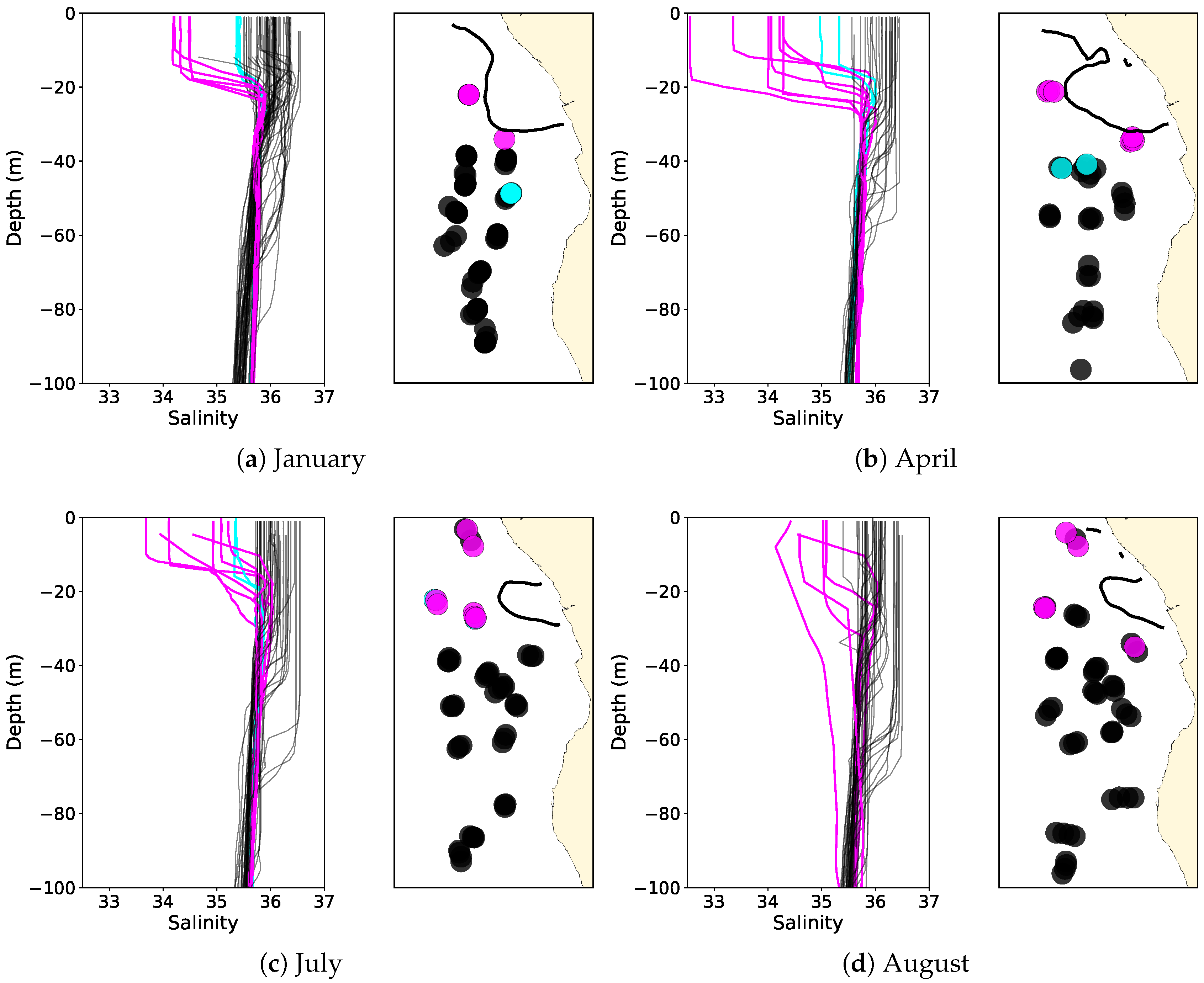
A total of 195 Argo float samples were taken in the Angola Basin over the entire 4 months analysed, providing independent data of salinity. However, none were located within the defined 34 PSU isohaline. Therefore in order to determine if some Argo floats were present within the Congo River plume, independent of a defined isohaline, a plume detection algorithm was used. Here, we follow Hopkins et al. [4], who used two main criteria (stratification and mean salinity less than the open ocean) to determine plume-detected Argo floats (Figure 3). Twenty-three samples (12%) were determined to be inside the plume (Pink lines and circles in Figure 3). By definition, stratification is present for all plume-detected Argo floats, meaning the comparison with SMOS sea surface salinity is robust. This small sample size is a partially a consequence of the expense of running a 4D-Var model system, and while more months and samples would have been ideal, the limited choice of months analysed was a computational restraint.
A persistence forecast was also included as a baseline forecast. An additional metric denoted the salinity skill score; , where AE_model (AE_persist) is the absolute error for the model (persistence) forecast, was computed to highlight improvements (ss>0) or degradation (ss<0) against persistence.
3. Results
3.1. Assimilation Analysis
The SMOS RMSE reduced for each experiment assimilating SMOS during the assimilation analysis as expected (Table 1). Interestingly, the combined assimilation SMOS SSH experiment had the smallest SMOS RMSE for three of the four months analysed, at 12–22% less than the SMOS experiment. The SMOS correlation coefficient (R) mirrored this result, exhibiting small improvements for SMOS SSH as compared to the SMOS only assimilation. Similarly, the SMOS RMSE and R also reduced and increased, respectively, for the SSH experiment as compared to the control for the majority of the study period. This result supports the benefits of altimetry assimilation in modelling the regional salinity field. Following this systemic reduction of SMOS errors, the data assimilation algorithm appears to be successfully fitting the salinity observations within the model.
The SMOS plume specific statistics (area, distance to the centre of mass, orientation and salinity within) also exhibits improvements for each month within the analysis (Table 2). Note this improvement is expected since we are assimilating and comparing against the same SMOS observations, and therefore solely representing whether the DA system can replicate the SMOS plume within the ROMS model.
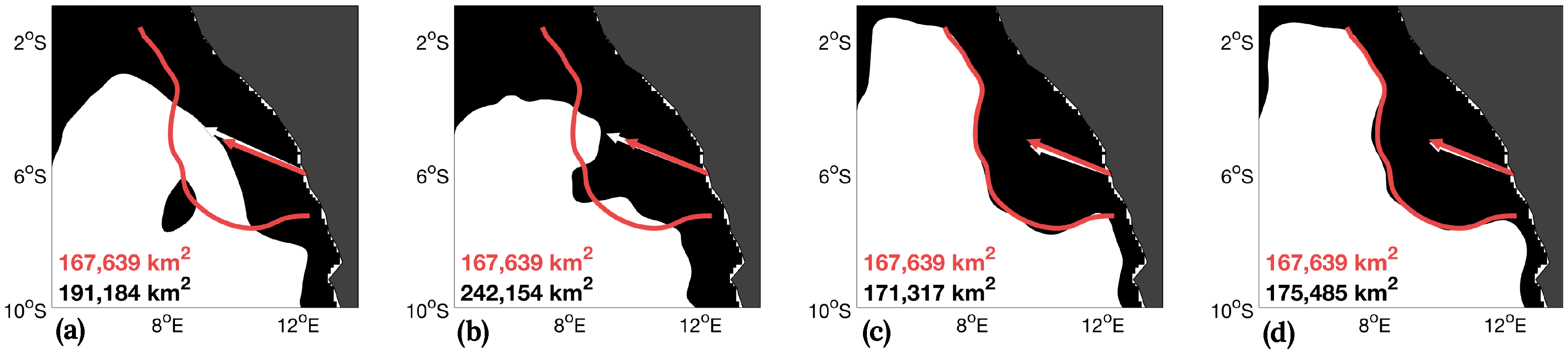
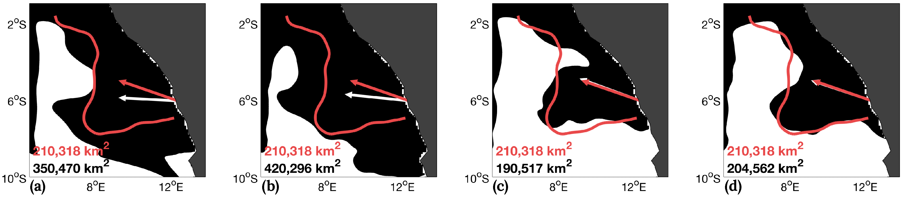
In the CNTRL experiment without assimilation, the plume experiences substantial biases for the majority of statistics (Table 2). For the area of the plume, the CNTRL is often vastly different than observed from SMOS. Figure 4 illustrates this bias for January (a month of high discharge) with an area mean absolute error (MAE) of around +27,000 km. Further discrepancies in the structure (stretched along the coast), orientation (2 MAE), distance to the centre of mass (80 km MAE) and average salinity within (2.5 PSU MAE) are present.
Contrary to improvements in the SMOS RMSE and R (Table 1), the subsequent assimilation of SSH does not always aid in significantly reducing this bias consistently across all months, sometimes enhancing it. For example, the January and April average plume area exhibit increased biases of up to 48,000 km (160%).
Only with the assimilation of SMOS (either alone or in combination with SSH) is the most systematic improvement over the CNTRL found across all months for the analysis. Most notably improving the area in the analysis by as much as 95% (visually represented in Figure 4). Here, the structure from SMOS is well replicated in the model analysis, resulting in improved orientation and distance to the centre of mass (95–100%). Note the additional benefits of assimilating both SMOS and SSH together for the analysis can be seen for many metrics. A summary statistic (final column in Table 2) confirms that the combined assimilation of SMOS and SSH is the best performing experiment for three of the four months analysed. Improving upon assimilating solely SMOS by 4–7% averaged across all metrics.
While the SMOS plume specific statistics confirm the model can effectively replicate the SMOS plume via the assimilation process, independent observations from Argo floats offer a more robust indication of performance (Table 3).
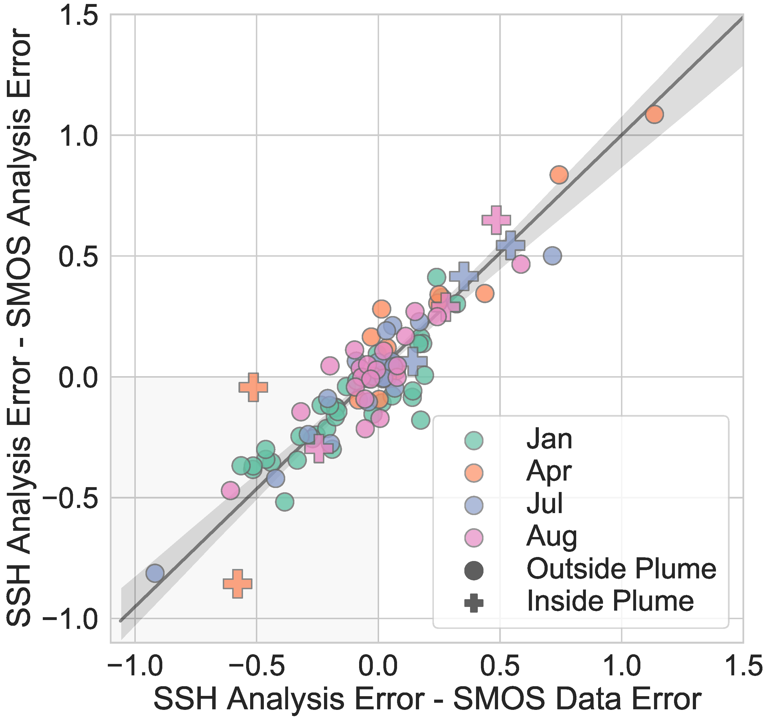
For the whole domain, the analysis for the SMOS assimilation experiment produced the smallest Argo MAE for April, July and August, improving over the CNTRL by 13% to 52%. For Argo floats inside the plume as identified by the algorithm as described in Hopkins et al. [4], the SMOS assimilation also produced the smallest Argo MAE comparisons. Curiously, the addition of the SSH, as in the combination of SMOS and SSH often increased errors for Argo float comparisons. Only for January did the additional assimilation of SSH decrease errors. This improvement is clearly because of superior performance of the SSH analysis (without SMOS). Possibly indicating that the assimilated SMOS data may be more inconsistent with the Argo floats, which carries through to the SMOS analysis. This relationship is shown in Figure 5. There is a strong significant correlation (, p-value < 0.01) between the SSH analysis–SMOS data error difference and SSH analysis–SMOS analysis error difference. Dividing the data into each month reveals that most of the January SSH Argo float errors (green circles in Figure 5) are smaller than that of the SMOS data and the SMOS analysis situated in the lower left hand shaded region (<0) within Figure 5.
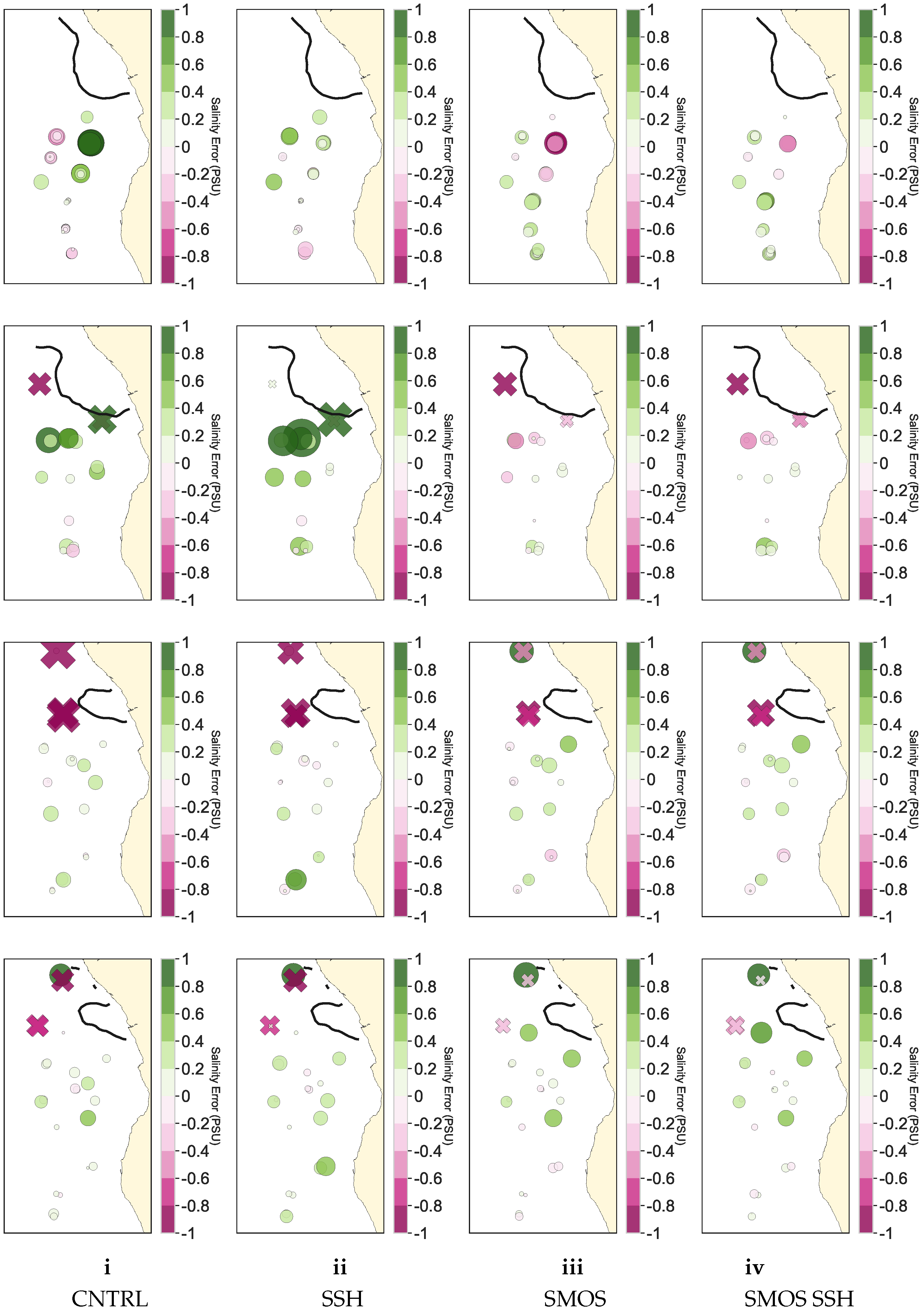
The spatial distribution of Argo floats present during the analysis is explored (Figure 6). For January (first row of Figure 6), very few Argo floats are located near the plume, with none independently determined to be inside the plume by the plume-detection algorithm (crosses in Figure 6). Here, the assimilation of SMOS appears to significantly increase errors further south as well as creating negative errors (the model is too saline) further north towards the coast. For April (second row in Figure 6), the CNTRL and SSH assimilation experiments exhibit a cluster of Argo floats with a substantial positive error (too fresh) around the centre of the model. The SMOS assimilation significantly reduces this cluster of errors. For July (third row in Figure 6), the SMOS assimilation slightly decreases large plume-detected Argo float errors in the north. Finally, August (final row in Figure 6) Argo floats exhibit a subtle change in errors from the CNTRL, with the SMOS assimilation reducing errors for the northernmost cluster that compose of the three plume-detected Argo floats.
3.2. Forecast
The 16-day forecasts initialised after the end of the final assimilation analysis cycle for each month also exhibited improvements over the CNTRL for SMOS plume specific statistics (Table 4). For higher discharge months (January and April), all metrics exhibit improvements over the CNTRL of up to 86% in the plume area, 54% in the distance to the centre of mass, 97% in orientation and 41% in salinity within. Conversely, for low discharge months (July and August), only minimal improvements are exhibited over the CNTRL for a handful of metrics, with degradation often present, notably during August. Despite improvements mainly limited to high discharge months, this result shows that the SMOS assimilation can maintain improvements from the analysis up to 16 days.
In combining SMOS with SSH, additional improvements are also exhibited for several plume metrics, more systematically for the forecast (Table 4) than as seen for the analysis period (Table 2). The plume area, for example, improves for an additional 10%, 4% and 17% during the January, April, and July forecast. This improvement is illustrated in Figure 7 with the structure of the plume better replicated for the SMOS SSH.
In addition to the model forecasts, a baseline of persistence was included. Since the SMOS dataset represents a 9-day moving average, good persistence skill in the plume statistics are highly likely, especially in an area with slowly evolving dynamics [23,36], where persistence forecast excels over 16 days [37].
Consequently, for many plume metrics over most months, the SMOS PERSIST forecast did indeed perform the best with the lowest errors and largest average improvement over the CNTRL (85–95%). So while SMOS or SMOS SSH assimilation forecast often outperforms the CNTRL, as seen in Figure 7, SMOS PERSIST is consistently better.
Again it is worth emphasising that the assessment of the SMOS plume specific statistics during the forecast are a measure of whether the model can retain improvements attained during the assimilation, rather than an independent validation of the forecast. This independent validation will instead be examined later for Argo floats present.
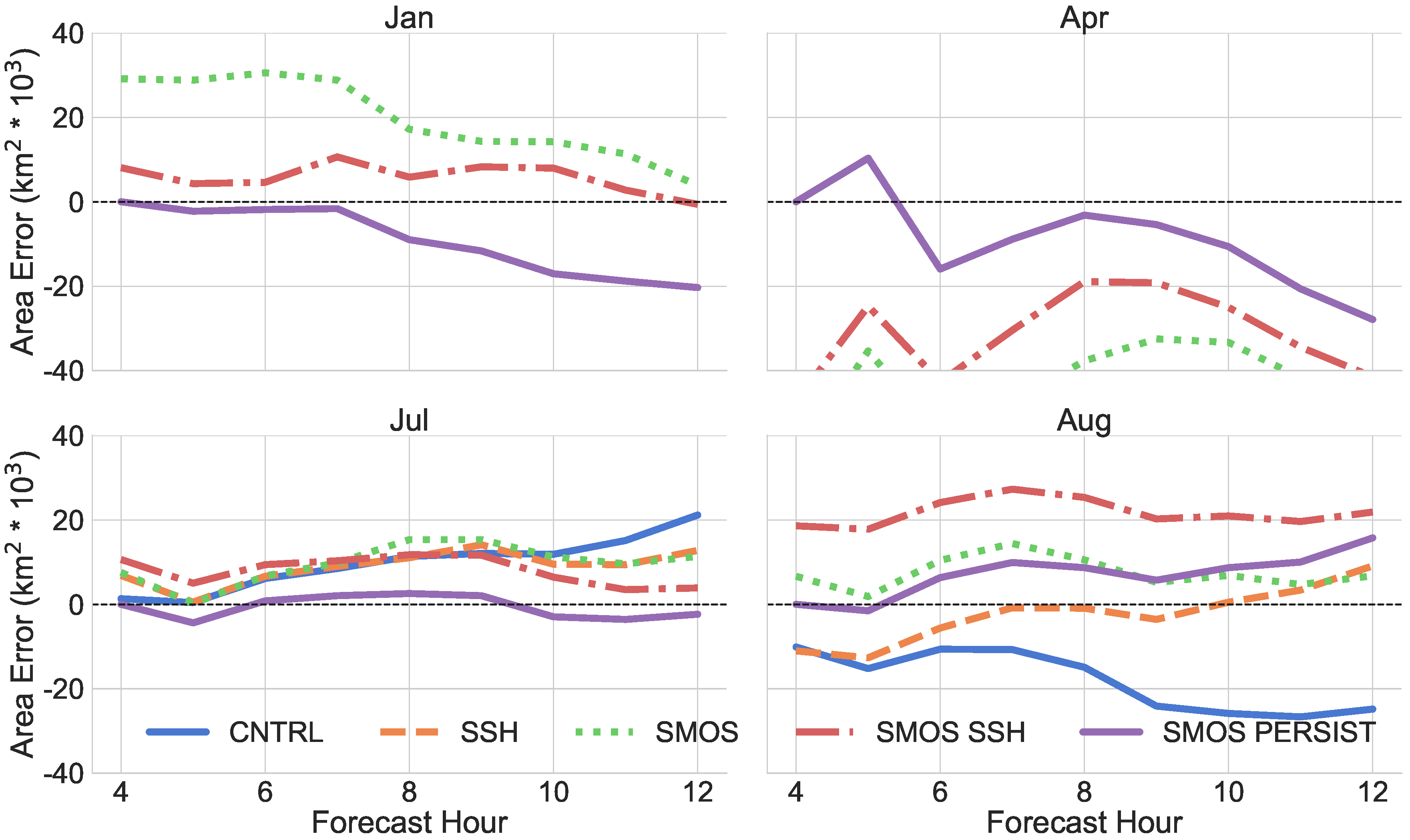
Nevertheless, the plume area statistics comes closest to showing some skill in these metrics beyond persistence. Figure 8 illustrates the time series of the plume area error for each experiment, split up into each month. For January and August, the SMOS SSH and SMOS assimilation forecast perform well, with persistence often exhibiting growing errors, contrary to the relatively stable model forecasts. For April and July, persistence is the most beneficial, with SMOS and SMOS SSH forecasts experiencing notable errors in April larger than −20,000 km.
Argo floats present for the forecast period can be used as an independent validation (Table 5). On average, for the whole domain, the Argo float MAE errors for the SMOS or SMOS SSH assimilation experiment were the smallest for three of the four months analysed. This result suggests that persistence has its limitations for independent data, and the SMOS assimilation forecast is valuable.
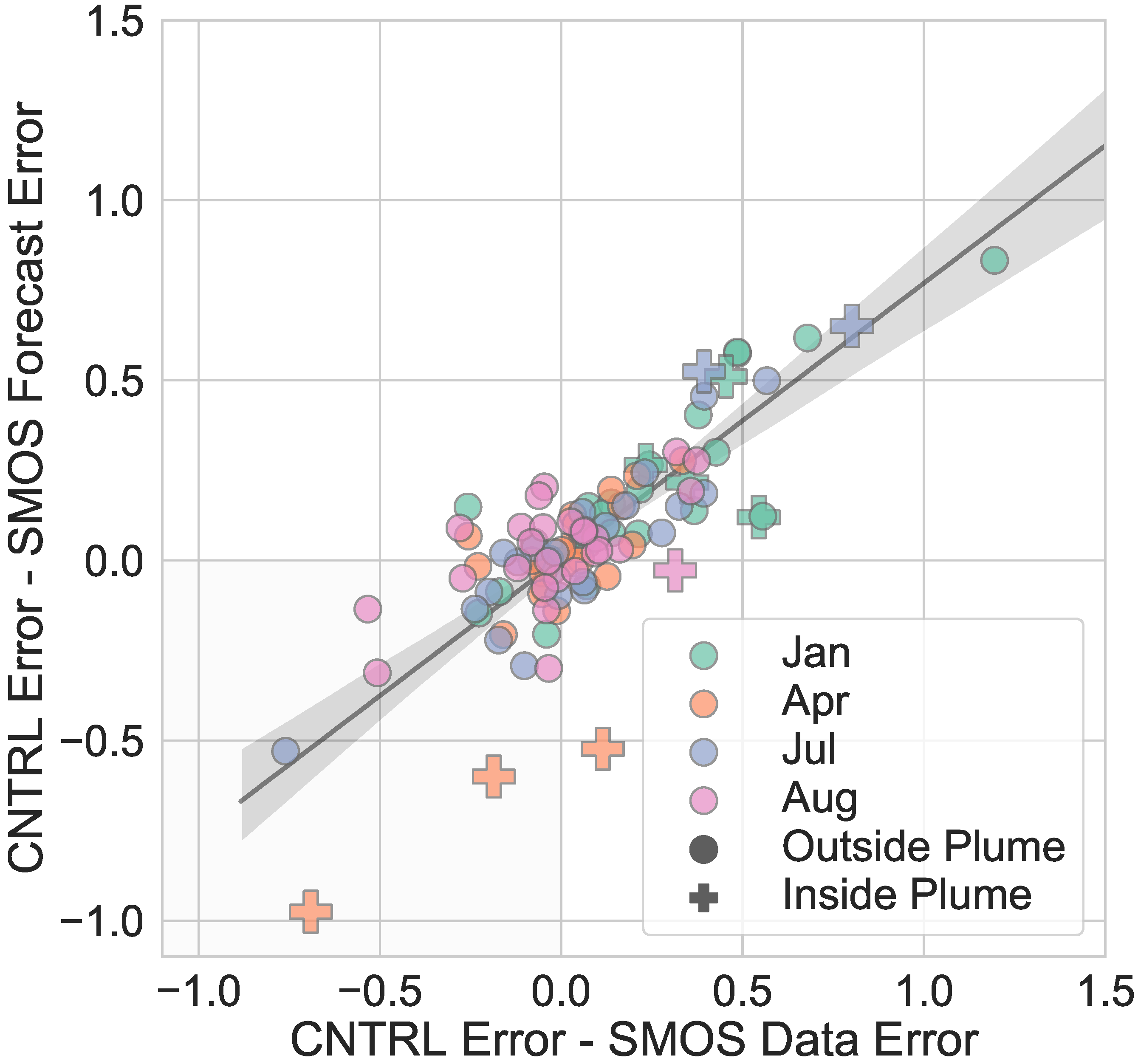
For January, the SMOS SSH assimilation forecast improves over the CNTRL by 60% and SMOS PERSIST by 14%. For plume-detected Argo floats this improvement is even more pronounced at 63% and 37%. For April, contrary to all previous indications, the CNTRL performs the best. The SMOS data during the April forecast period validates with the Argo floats relatively poorly with an MAE of 0.28 PSU, slightly larger than the CNTRL error at 0.27 PSU. It follows that the CNTRL model is more likely to outperform the SMOS forecast, where a strong correlation (0.93 < 0.05) between the CNTRL-SMOS data error difference and CNTRL–SMOS forecast error difference exists (Figure 9). This poor performance is even more apparent for Argo floats inside the plume, where the CNTRL improves over the SMOS forecast by 44%. This degradation in performance is similar to the analysis January period (Table 3), where the SMOS data was found to contain larger errors than the SSH analysis, and thus the resulting SMOS analysis performed inadequately. For July, the SMOS assimilation forecast has the smallest whole domain Argo float MAE, improving over the CNTRL by 36% and over persistence by 28%. The two plume-detected Argo floats also exhibited this trend improving over the CNTRL and persistence by 70% and 10% respectively. Finally, for August, the SMOS assimilation forecast had the smallest Argo float MAE, improving over the control by 13%. Although, the difference between the CNTRL, SMOS forecast, SMOS SSH forecast and SMOS persistence was minimal from 0.01 to 0.04 PSU. A single Argo float was determined to be inside the plume during the August forecast. The location was very close to the edge of the model domain, where boundary errors dominate the model results. Therefore persistence performed well as expected.
We now focus on the spatial distribution of forecast errors for the Argo floats across the domain. Furthermore, we alternatively present the skill score against persistence (Figure 10). Positive values represent improvements over persistence (green triangles), while negative values (purple circles) indicate degradation over persistence. Green pluses and purple crosses are used as an alternative representation for plume-detected Argo floats.
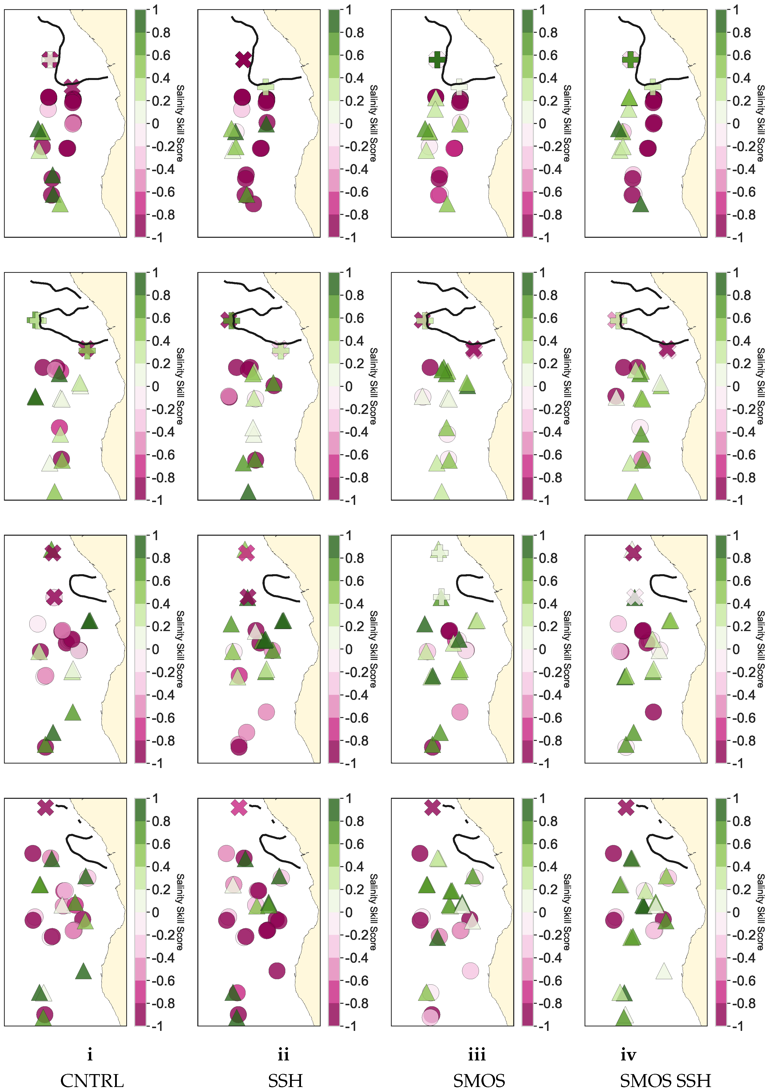
For January (first row of Figure 10), the CNTRL cannot outperform persistence for the majority of the Argo float samples, especially in the north, towards the plume. The SMOS assimilation forecast mostly corrects this, with some Argo floats remaining favoured towards persistence. For April (second row of Figure 10), the CNTRL is the best performing forecast for the majority of Argo floats. The forecast from the assimilation of SMOS does not significantly improve results with both improvements and degradation present. For July (third row of Figure 10), systematic improvements are seen for the assimilation of SSH and SMOS forecast. Interestingly, the improvement of SSH forecast can almost replicate the improvements as seen in the SMOS forecast. Improvements in the circulation are likely contributing to improvements in salinity advection. However, only the SMOS forecast can dramatically improve the plume-detected Argo floats in the north of the domain. Finally, for August (final row of Figure 10), improvements for the SMOS assimilation are mostly exhibited for the central cluster of Argo floats as compared to the CNTRL.
For every Argo float sample available during each month’s forecast period (104 in total) the percentage of forecast skill scores above zero (positive values) can be computed. This represents the portion of persistence favoured Argo floats as compared to each experiment forecast. For example, the SMOS and SMOS SSH assimilation forecast contain 55% positive skill scores. This proportion split means these forecasts are 5% more likely to outperform persistence. Much larger than both the CNTRL and SSH experiments at approximately 40%, meaning that persistence is instead 10% more likely to outperform these forecasts.
4. Discussion
The CNTRL and SSH assimilation experiments inadequately reproduced observations of the Congo River plume (via SMOS plume statistics and Argo float comparisons). A few hypotheses can be put forth to explain this deficiency. Firstly, the discharge of the plume may be incorrect. The river input is based on 103 years of data which ends in 2005 (Figure 2). The standard deviations for this dataset range from only 10–15% of the mean value. The discharge error is thus unlikely to account for the extreme differences between the observations and the control. Deficiencies in the mixing schemes and resolution could limit the plume simulation, especially near the river mouth. The Angola Basin ROMS model has a resolution of 10 km with two grid points representing the opening of the Congo River channel Recently, Bars et al. [15] employed a multi-scale unstructured mesh model to simulate the Congo river-to-sea continuum, with elements as small as 200 m in the river and estuary and as large 20 km in the deep ocean. They note the river flow is characterised by smaller length scales that require a higher resolution. Therefore, it is clear that the resolution of the Congo within Angola Basin ROMS could be restricting the mixing of freshwater, and thus enabling a very fresh bias to expand into the open ocean where the general ocean circulation could propagate the bias into the basin. Furthermore, extreme gradients in the bathymetry such as those found near the Congo Canyon (originating downstream of the river) are particularly challenging [15]. The surface forcing from ERA-I could also generate errors. For example, local 10 m winds not correctly captured within ERA-I could result in erroneous currents that inaccurately advect the plume. Total precipitation errors will also affect the upper ocean salinity. This changes the evaporation minus precipitation (E-P) value that determines the net flux of freshwater into the ocean. Finally, the boundary conditions from HYCOM could contain an inaccurate salinity field that is propagating into the domain. However, despite these apparent difficulties, the assimilation of SMOS can successfully constrain the plume and adjust any prior bias in the model salinity as seen in the control.
Either the SMOS or SMOS SSH experiments performed the best for the majority of metrics in the analysis and forecast. It is well documented that the assimilation of SSH improves the large-scale ocean circulation [38,39,40,41,42] and this, in turn, could become especially important for the forecast of the plume with the improved currents spreading the adjusted plume (via the SMOS assimilation) more realistically. The free-running model forecast is no longer constrained by the regular daily SMOS assimilation and instead relies on the dynamics of the circulation spreading the far-field plume. While this suggests the assimilation of solely SSH should also improve the plume, deficiencies in CNTRL plume structure are likely already too large to correct from the adjustments in circulation patterns and multivariate correlations in the background error covariance.
Several Argo floats were crucially available throughout the domain for independent verification during each month. The SMOS assimilation analysis and forecasts performed the best most months analysed with the smallest Argo float errors. The addition of the SSH, as in the combined assimilation of SMOS with SSH, often slightly degraded the results. A hypothesis for this degradation is related to the relative weighting of the observations and model within the 4D-Var system. Most Argo float samples were located further away from the plume, where the standard deviation of the model climatology simulation drops below 0.2 PSU (not shown). Therefore with a 1.2 PSU SMOS observation error, the cost function is heavily weighted towards the model, only subtly changing the sea surface salinity field within the model, while also adjusting the salinity field via the multivariate balance options and, the evolution of the tangent linear (TL) and adjoint (AD) models from the SSH assimilation. This is the limitation of using a static covariance matrix within 4D-Var. Advanced hybrid methodologies (Hybrid-4DVar) are likely to improve results. Usually this involves replacing the static background error covariance matrix with an ensemble covariance computed from using an ensemble of non-linear model runs at each assimilation time [43]. Implementing this system into ROMS IS4D-Var is beyond the scope of this study.
While a simple persistence forecast proved to be a good predictor of the majority of plume statistics (computed from the SMOS data), persistence could not provide an adequate forecast for the Argo floats. However, it was found that when the SMOS data validated poorly against the Argo floats during the analysis (forecast) period, as compared to the CNTRL or SSH analysis (forecast), the SMOS or SMOS SSH analysis (forecast) also performed poorly. While this result is somewhat trivial, it is vital to note that the capability of the model is intrinsically linked to the quality of the data.
The difference in the temporal resolution between the Argo floats, and SMOS data could explain the discrepancy in this comparison. The Argo floats represent the surface salinity at a much shorter time scales than the SMOS data (a 9-day moving average product). Therefore, the plume’s extent is highly likely to be underestimated, and details near the plume will not be captured [4]. Still, despite this clear limitation, the SMOS forecast performed well for the majority of months analysed.
Lu et al. [18] showed that for the assimilation of SMOS the root mean squared error (RMSE) of the modelled sea surface salinity field compared with Argo float salinity data within the tropics (20 S–20 N) reduced by approximately 30% as compared to a control. This result held only for the open ocean as Lu et al. [18] used an older version of the BEC data [44]. Nevertheless, an improvement in the model when assimilating SMOS is similarly found in the experiments presented in this study. Köhl et al. [19] assimilated a different SMOS product (processed by the University of Hamburg) globally but found conflicting results to Lu et al. [18] and this study (negative to neutral impacts on the salinity field for the open ocean). Lu et al. [18] noted differences in the observation error covariance, models and data assimilation methods and SMOS datasets as possible reasons for this discrepancy. Finally, Mu et al. [21] recently assimilated a bias-corrected version of the updated SMOS dataset. They found up to 70% improvements with an RMSE less than 0.1 PSU, although it should be noted that their control RMSE was initially 0.3 PSU, smaller than the control for this study (RMSE errors of 0.4-0.7 PSU).
5. Conclusions
A first attempt of assimilating satellite salinity to model a major river plume has been presented. The latest version of SMOS, a satellite salinity product, was recently (2017) processed with an updated technique to reduce errors near the coast. This allows more frequent coastal data, which could be employed in a DA system of the Congo River plume. The ROMS Angola Basin configuration with IS4D-Var assimilated SSH, SMOS or SMOS SSH combined for four months.
The metrics applied to assess the assimilation analysis revealed that the SMOS observations were successfully assimilated during each month and maintained improvements throughout a subsequent forecast. The SMOS structure was well replicated within the model with regards to the plume area, distance to the centre of mass, orientation and average salinity within. Independent Argo float salinity profiles were available during the months analysed. The MAE of the Argo floats during the majority of months analysed reduced as compared to the control and persistence with the assimilation of SMOS. There are limitations to the current model, which are most likely due to a higher horizontal resolution required to resolve the upstream plume mixing. However, it has been shown that the current generation of satellite salinity observations can be successfully used to constrain a large river plume such as that produced by the Congo River. This successful assimilation stage could be the first step in producing operational forecasts of river plumes in the future.
Author Contributions
L.P. and R.T. conceived and designed the experiments. L.P. performed the experiments, analysis and wrote the paper. R.T provided insights and guidance, as well as contributing to the writing-review and editing of the paper. All authors have read and agreed to the published version of the manuscript.
Funding
This research was funded by the Natural Environment Research Council (NERC) award reference 1660325.
Acknowledgments
This study was supported by the Natural Environment Research Council (NERC). The authors would like to thank the Imperial College High Performance Computing Service (10.14469/hpc/2232) for providing computational resources. The altimeter products were produced by Ssalto/Duacs and distributed by Aviso, with support from Cnes (http://www.aviso.altimetry.fr/duacs/). Argo float data were collected and made freely available by the International Argo Program and the national programs that contribute to it (http://www.argo.ucsd.edu, http://argo.jcommops.org). The Argo Program is part of the Global Ocean Observing System (http://0-doi-org.brum.beds.ac.uk/10.17882/42182). We thank two anonymous reviewers whose constructive comments improved the manuscript.
Conflicts of Interest
The authors declare no conflict of interest.
References
- Dagg, M.; Benner, R.; Lohrenz, S.; Lawrence, D. Transformation of dissolved and particulate materials on continental shelves influenced by large rivers: Plume processes. Cont. Shelf Res. 2004, 24, 833–858. [Google Scholar] [CrossRef]
- Chen, C.T.A.; Zhai, W.; Dai, M. Riverine input and air-sea CO2 exchanges near the Changjiang (Yangtze River) Estuary: Status quo and implication on possible future changes in metabolic status. Cont. Shelf Res. 2008, 28, 1476–1482. [Google Scholar] [CrossRef]
- Kang, Y.; Pan, D.; Bai, Y.; He, X.; Chen, X.; Chen, C.T.A.; Wang, D. Areas of the global major river plumes. Acta Oceanol. Sin. 2013, 32, 79–88. [Google Scholar] [CrossRef]
- Hopkins, J.; Lucas, M.; Dufau, C.; Sutton, M.; Stum, J.; Lauret, O.; Channelliere, C. Detection and variability of the Congo River plume from satellite derived sea surface temperature, salinity, ocean colour and sea level. Remote. Sens. Environ. 2013, 139, 365–385. [Google Scholar] [CrossRef]
- Braga, E.S.; Andrié, C.; Bourlès, B.; Vangriesheim, A.; Baurand, F.; Chuchla, R. Congo River signature and deep circulation in the eastern Guinea Basin. Deep-Sea Res. Part I Oceanogr. Res. Pap. 2004, 51, 1057–1073. [Google Scholar] [CrossRef]
- Higgins, H.W.; Mackey, D.J.; Clementson, L. Phytoplankton distribution in the Bismarck Sea north of Papua New Guinea: The effect of the Sepik River outflow. Deep-Sea Res. Part I Oceanogr. Res. Pap. 2006, 53, 1845–1863. [Google Scholar] [CrossRef]
- Kouame, K.; Yapo, O.; Mambo, V.; Seka, A.; Tidou, A.; Houenou, P. Physicochemical Characterization of the Waters of the Coastal Rivers and the Lagoonal System of Cote d‘Ivoire. J. Appl. Sci. 2009, 9, 1517–1523. [Google Scholar] [CrossRef]
- Yankovsky, A.E.; Chapman, D.C. A simple theory for the fate of buoyant coastal discharges. J. Phys. Oceanogr. 1997, 27, 1386–1401. [Google Scholar] [CrossRef] [Green Version]
- Eisma, D.; van Bennekom, A.J. The Zaire river and estuary and the Zaire outflow in the Atlantic Ocean. Neth. J. Sea Res. 1978, 12, 255–272. [Google Scholar] [CrossRef]
- Denamiel, C.; Budgell, W.P.; Toumi, R. The congo river plume: Impact of the forcing on the far-field and near-field dynamics. J. Geophys. Res. Ocean. 2013, 118, 964–989. [Google Scholar] [CrossRef]
- Signorini, S.R.; Murtugudde, R.G.; McClain, C.R.; Christian, J.R.; Picaut, J.; Busalacchi, A.J. Biological and physical signatures in the tropical and subtropical Atlantic. J. Geophys. Res. Ocean. 1999, 104, 18367–18382. [Google Scholar] [CrossRef] [Green Version]
- Vic, C.; Berger, H.; Tréguier, A.M.; Couvelard, X. Dynamics of an Equatorial River Plume: Theory and Numerical Experiments Applied to the Congo Plume Case. J. Phys. Oceanogr. 2014, 44, 980–994. [Google Scholar] [CrossRef] [Green Version]
- Palma, E.D.; Matano, R.P. An idealized study of near equatorial river plumes. J. Geophys. Res. Ocean. 2017, 122, 3599–3620. [Google Scholar] [CrossRef]
- White, R.H.; Toumi, R. River flow and ocean temperatures: The Congo River. J. Geophys. Res. Ocean. 2014, 119, 2501–2517. [Google Scholar] [CrossRef]
- Bars, Y.L.; Vallaeys, V.; Deleersnijder, É.; Hanert, E.; Carrere, L.; Channelière, C. Unstructured-mesh modeling of the Congo river-to-sea continuum. Ocean. Dyn. 2016, 66, 589–603. [Google Scholar] [CrossRef]
- Liu, Y.; MacCready, P.; Hickey, B.M.; Dever, E.P.; Kosro, P.M.; Banas, N.S. Evaluation of a coastal ocean circulation model for the Columbia River plume in summer 2004. J. Geophys. Res. Ocean. 2009, 114, C00B04. [Google Scholar] [CrossRef] [Green Version]
- Lahoz, W.; Khattatov, B.; Ménard, R. Data assimilation and information. In Data Assimilation: Making Sense of Observations, 1st ed.; Lahoz, W., Khattatov, B., Menard, R., Eds.; Springer: Berlin/Heidelberg, Germany, 2010; Chapter 1; pp. 3–12. [Google Scholar]
- Lu, Z.; Cheng, L.; Zhu, J.; Lin, R. The complementary role of SMOS sea surface salinity observations for estimating global ocean salinity state. J. Geophys. Res. Ocean. 2016, 121, 3672–3691. [Google Scholar] [CrossRef]
- Köhl, A.; Sena Martins, M.; Stammer, D. Impact of assimilating surface salinity from SMOS on ocean circulation estimates. J. Geophys. Res. Ocean. 2014, 119, 5449–5464. [Google Scholar] [CrossRef]
- Olmedo, E.; Martínez, J.; Turiel, A.; Ballabrera-Poy, J.; Portabella, M. Debiased non-Bayesian retrieval: A novel approach to SMOS Sea Surface Salinity. Remote. Sens. Environ. 2017, 193, 103–126. [Google Scholar] [CrossRef]
- Mu, Z.; Zhang, W.; Wang, P.; Wang, H.; Yang, X. Assimilation of SMOS sea surface salinity in the regional ocean model for South China Sea. Remote. Sens. 2019, 11, 919. [Google Scholar] [CrossRef] [Green Version]
- Moore, A.M.; Arango, H.G.; Broquet, G.; Edwards, C.; Veneziani, M.; Powell, B.; Foley, D.; Doyle, J.D.; Costa, D.; Robinson, P. The Regional Ocean Modeling System (ROMS) 4-dimensional variational data assimilation systems. Part III—Observation impact and observation sensitivity in the California Current System. Prog. Oceanogr. 2011, 91, 74–94. [Google Scholar] [CrossRef]
- Phillipson, L.; Toumi, R. Impact of data assimilation on ocean current forecasts in the Angola Basin. Ocean. Model. 2017, 114, 45–58. [Google Scholar] [CrossRef]
- Chassignet, E.P.; Hurlburt, H.E.; Smedstad, O.M.; Halliwell, G.R.; Hogan, P.J.; Wallcraft, A.J.; Baraille, R.; Bleck, R. The HYCOM (HYbrid Coordinate Ocean Model) data assimilative system. J. Mar. Syst. 2007, 65, 60–83. [Google Scholar] [CrossRef]
- Dee, D.P.; Uppala, S.M.; Simmons, A.J.; Berrisford, P.; Poli, P.; Kobayashi, S.; Andrae, U.; Balmaseda, M.A.; Balsamo, G.; Bauer, P.; et al. The ERA-Interim reanalysis: Configuration and performance of the data assimilation system. Q. J. R. Meteorol. Soc. 2011, 137, 553–597. [Google Scholar] [CrossRef]
- Vorosmarty, C.; Fekete, B.M.; Tucker, B. Global River Discharge, 1807–1991, V. 1.1 (RivDIS); Oak Ridge Natl. Lab. Distrib. Active Arch. Cent.: Oak Ridge, TN, USA, 1998. [Google Scholar]
- Meybeck, M.; Ragu, A. GEMS-GLORI World River Discharge Database; Lab. de Gologie Appl., Univ. Pierre et Marie Curie: Paris, France, 2012. [Google Scholar]
- Alsdorf, D.; Beighley, E.; Laraque, A.; Lee, H.; Tshimanga, R.; O’Loughlin, F.; Mahé, G.; Dinga, B.; Moukandi, G.; Spencer, R.G.M. Opportunities for hydrologic research in the Congo Basin. Rev. Geophys. 2016, 54, 378–409. [Google Scholar] [CrossRef] [Green Version]
- Jackson, B.; Nicholson, S.E.; Klotter, D. Mesoscale Convective Systems over Western Equatorial Africa and Their Relationship to Large-Scale Circulation. Mon. Weather. Rev. 2009, 137, 1272–1294. [Google Scholar] [CrossRef]
- Phillipson, L. Ocean Data Assimilation in the Angola Basin. Ph.D. Thesis, Imperial College London, London, UK, 2018. [Google Scholar]
- SMOS-BEC Team. Quality Report: Validation of Debiased Non-Bayesian BEC advanced Sea Surface Salinity Products; Technical Report; Barcelona Expert Centre: Barcelona, Spain, 2017. [Google Scholar]
- Willis, J.K. Interannual variability in upper ocean heat content, temperature, and thermosteric expansion on global scales. J. Geophys. Res. 2004, 109, C12036. [Google Scholar] [CrossRef] [Green Version]
- Good, S.A.; Martin, M.J.; Rayner, N.A. EN4: Quality controlled ocean temperature and salinity profiles and monthly objective analyses with uncertainty estimates. J. Geophys. Res. Ocean. 2013, 118, 6704–6716. [Google Scholar] [CrossRef]
- Weaver, A.T.; Deltel, C.; Machu, E.; Ricci, S.; Daget, N. A multivariate balance operator for variational ocean data assimilation. Q. J. R. Meteorol. Soc. 2006, 131, 3605–3625. [Google Scholar] [CrossRef] [Green Version]
- Moore, A.M.; Edwards, C.A.; Fiechter, J.; Drake, P.; Neveu, E.; Arango, H.G.; Gürol, S.; Weaver, A.T. A 4D-var analysis system for the california current: A prototype for an operational regional ocean data assimilation system. In Data Assimilation for Atmospheric, Oceanic and Hydrologic Applications (Vol. II); Springer: Berlin/Heidelberg, Germany, 2013; pp. 345–366. [Google Scholar]
- Lumpkin, R.; Johnson, G.C. Global ocean surface velocities from drifters: Mean, variance, El Niño–Southern Oscillation response, and seasonal cycle. J. Geophys. Res. Ocean. 2013, 118, 2992–3006. [Google Scholar] [CrossRef]
- Phillipson, L.M.; Toumi, R. The Crossover Time as an Evaluation of Ocean Models Against Persistence. Geophys. Res. Lett. 2018, 45, 250–257. [Google Scholar] [CrossRef] [Green Version]
- Fukumori, I.; Raghunath, R.; Fu, L.L.; Chao, Y. Assimilation of TOPEX/Poseidon altimeter data into a global ocean circulation model: How good are the results? J. Geophys. Res. Ocean. 1999, 104, 25647–25665. [Google Scholar] [CrossRef]
- Dorofeev, V.L.; Korotaev, G.K. Assimilation of the data of satellite altimetry in an eddy-resolving model of circulation of the Black Sea. Phys. Oceanogr. 2004, 14, 42–56. [Google Scholar] [CrossRef]
- Dombrowsky, E.; Bertino, L.; Brassington, G.; Chassignet, E.; Davidson, F.; Hurlburt, H.; Kamachi, M.; Lee, T.; Martin, M.; Mei, S.; et al. GODAE Systems in Operation. Oceanography. 2009, 22, 80–95. [Google Scholar] [CrossRef] [Green Version]
- Moore, A.M.; Arango, H.G.; Broquet, G.; Edwards, C.; Veneziani, M.; Powell, B.; Foley, D.; Doyle, J.D.; Costa, D.; Robinson, P. The Regional Ocean Modeling System (ROMS) 4-dimensional variational data assimilation systems. Part II—Performance and application to the California Current System. Prog. Oceanogr. 2011, 91, 50–73. [Google Scholar] [CrossRef]
- Da Rocha Fragoso, M.; de Carvalho, G.V.; Soares, F.L.M.; Faller, D.G.; de Freitas Assad, L.P.; Toste, R.; Sancho, L.M.B.; Passos, E.N.; Böck, C.S.; Reis, B.; et al. A 4D-variational ocean data assimilation application for Santos Basin, Brazil. Ocean. Dyn. 2016, 66, 419–434. [Google Scholar] [CrossRef]
- Desroziers, G.; Camino, J.T.; Berre, L. 4DEnVar: Link with 4D state formulation of variational assimilation and different possible implementations. Q. J. R. Meteorol. Soc. 2014, 140, 2097–2110. [Google Scholar] [CrossRef]
- Font, J.; Boutin, J.; Reul, N.; Spurgeon, P.; Ballabrera-Poy, J.; Chuprin, A.; Gabarró, C.; Gourrion, J.; Guimbard, S.; Hénocq, C.; et al. SMOS first data analysis for sea surface salinity determination. Int. J. Remote. Sens. 2013, 34, 3654–3670. [Google Scholar] [CrossRef]
Figure 1.
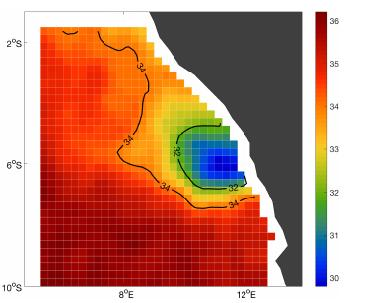
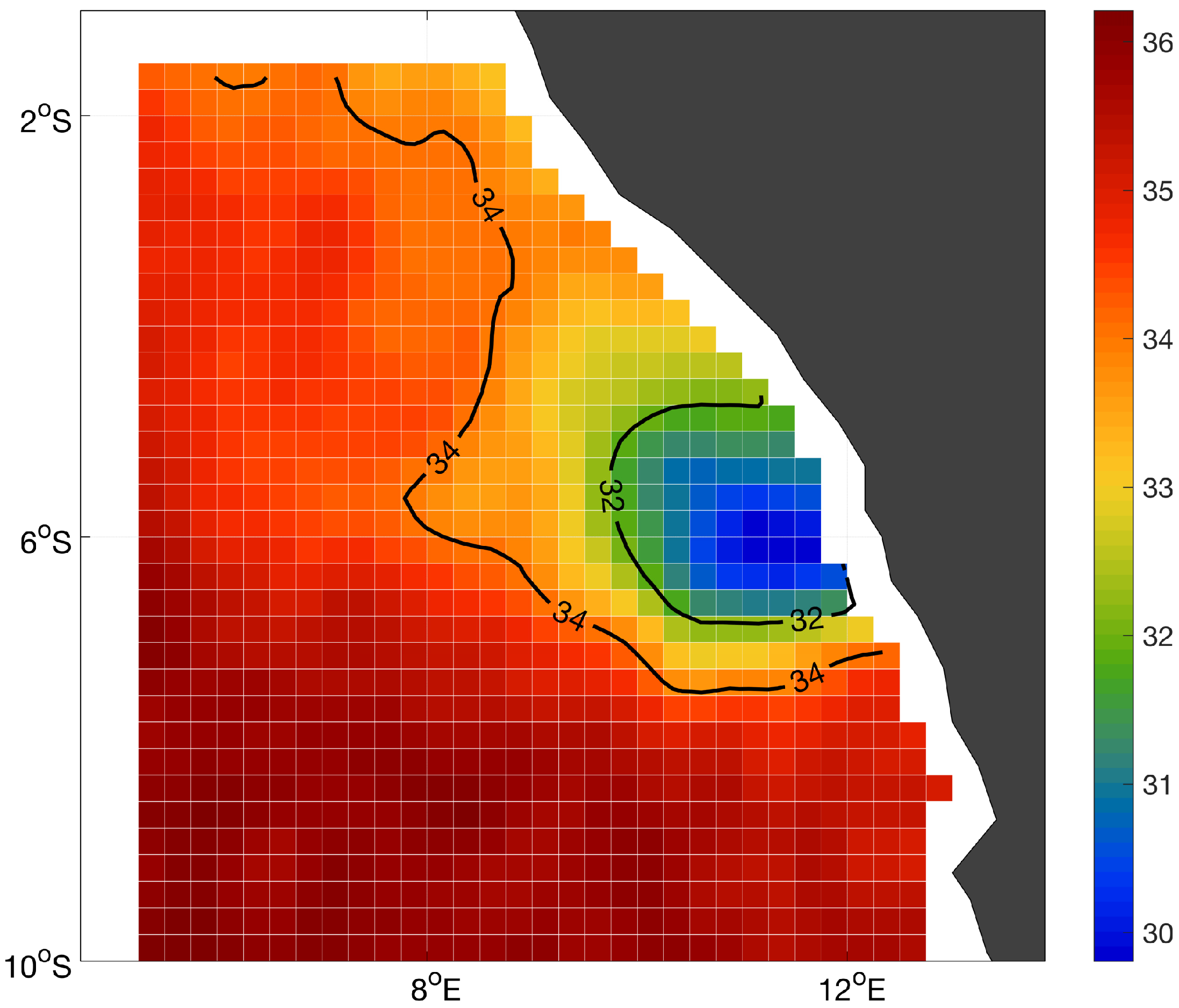
A snapshot of the 2017 Soil Moisture and Ocean Salinity (SMOS) data from the Barcelona Expert Centre (BEC) [20] for January 2013 with filled salinity (PSU), and the 32 PSU and 34 PSU isohaline (lines of constant salinity) in black.
Figure 1.
A snapshot of the 2017 Soil Moisture and Ocean Salinity (SMOS) data from the Barcelona Expert Centre (BEC) [20] for January 2013 with filled salinity (PSU), and the 32 PSU and 34 PSU isohaline (lines of constant salinity) in black.

Figure 2.
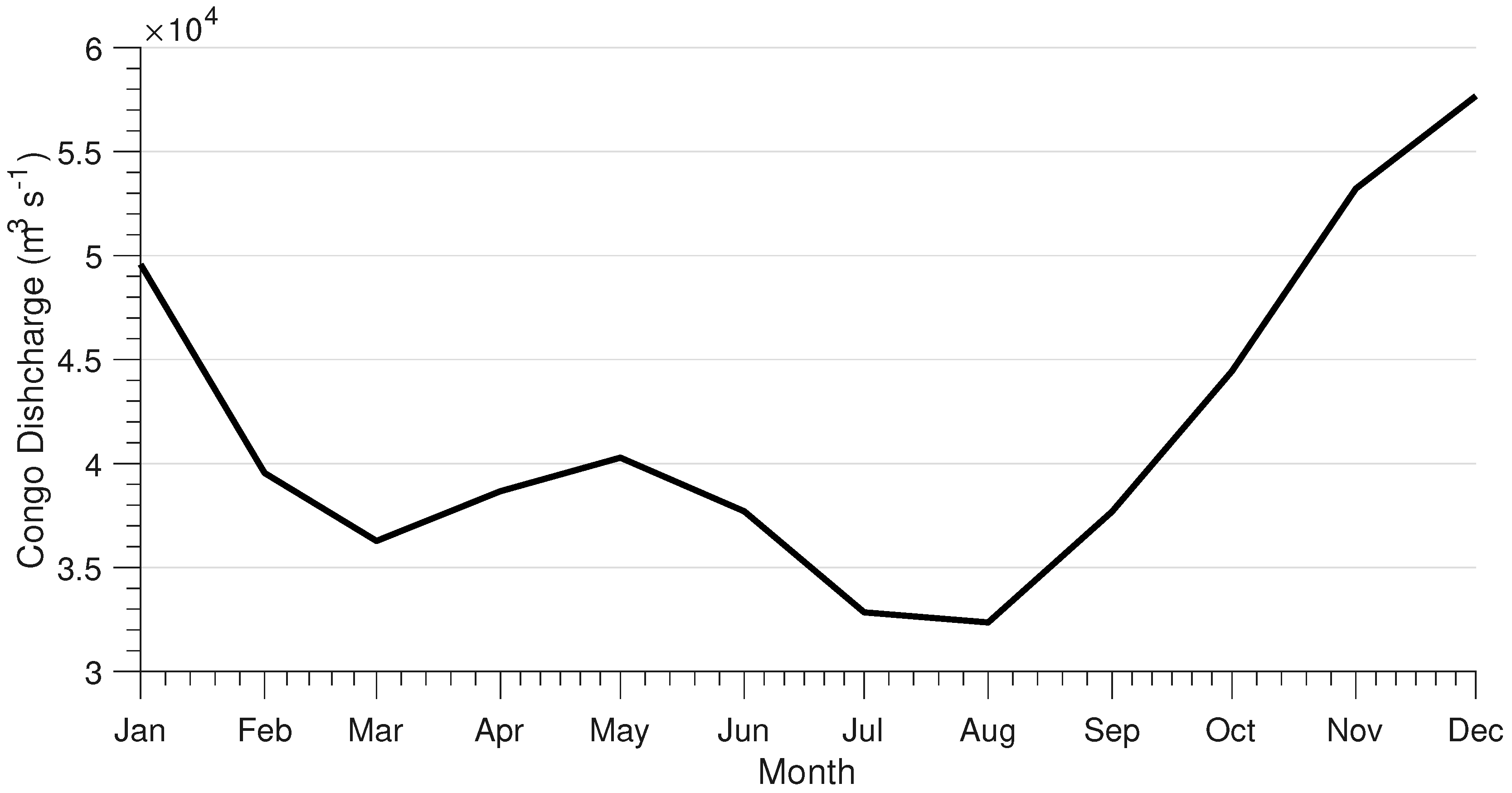
The average annual cycle of the Congo River discharge used within the model. The average is calculated from the observed monthly mean discharge between 1902 and 2005 provided by the BEI ERE in collaboration with the University of Brazzaville. Adapted from Phillipson [30].
Figure 2.
The average annual cycle of the Congo River discharge used within the model. The average is calculated from the observed monthly mean discharge between 1902 and 2005 provided by the BEI ERE in collaboration with the University of Brazzaville. Adapted from Phillipson [30].

Figure 3.
Argo float salinity profiles for top 100 meters (left) and their associated locations (right) during (a) January, (b) April, (c) July and (d) August. Black profiles and circles represent Argo floats determined to be outside the plume according to the plume detection algorithm. Purple profiles and circles represent Argo floats determined to be inside the plume. Blue profiles and circles represent Argo floats that only meet one criteria from the plume detection algorithm. Overlaid in black are the average 34 PSU isohalines for each respective month.

Figure 4.
The 34 PSU plume area for (a) the control (CNTRL), (b) sea surface height (SSH), (c) SMOS and (d) SMOS SSH assimilation analysis (black filled) and SMOS data (red outlines) averaged for the January analysis. Overlaid are arrows denoting the orientation and distance to centre of mass for each experiment (white) and the SMOS data (red). The bottom left numbers denote the area of the plume for each experiment (black) and SMOS data (red).

Figure 5.
A scatter plot of the Argo float SSH analysis error minus the Argo float SMOS analysis error against the Argo float SSH analysis error minus the Argo float SMOS data error. The data is split into each study month, January (green), April (orange), July (blue) and August (pink). Outside (inside) plume samples are represented as circles (pluses). A linear regression is overlaid with a shaded bootstrap confidence interval. An additional shaded area for values <0 is displayed to highlight Argo float SSH analysis errors that outperform both the SMOS analysis and SMOS data.

Figure 6.
The Argo float surface salinity errors over the January (1st row), April (2nd row), July (3rd row) and August (4th row) analysis for experiments (i) CNTRL, (ii) SSH, (iii) SMOS and (iv) SMOS SSH. In addition to the caxis colour scale representing negative (purple) to positive (green) salinity bias (PSU), smaller circle sizes represent smaller biases. Crosses (instead of circles) are alternatively displayed to represent the plume detected samples as seen in Figure 3. The average 34 PSU isohaline computed from the SMOS data for each respective month (analysis period) is overlaid in black.

Figure 7.
The 34 PSU plume area for (a) the control (CNTRL), (b) sea surface height (SSH), (c) SMOS and (d) SMOS SSH assimilation forecast (black filled) and SMOS data (red outlines) averaged for the January forecast. Overlaid are arrows denoting the orientation and distance to centre of mass for each experiment (white) and the SMOS data (red). The bottom left numbers denote the area of the plume for each experiment (black) and the SMOS data (red).

Figure 8.
The plume area error as a function of forecast time, split into the four months for each forecast; CNTRL (blue solid line), SSH (yellow dashed line), SMOS (green dotted line), SMOS SSH (red dashed dot line) and SMOS PERSIST (purple solid line). A black dashed line highlights the zero error mark. Note the day four starting date is due to the computation of a 9-day moving average for the model forecast. This average enables an appropriate comparison with the SMOS data set. Forecasts not displayed within a certain month, indicate the errors are beyond the axis limits (−40,000 to 40,000 km), as in January and April for the CNTRL and SSH forecasts.

Figure 9.
A scatter plot of the Argo float CNTRL error minus the Argo float SMOS forecast error against the Argo float CNTRL error minus the Argo float SMOS data error. The data is split into each study month, January (green), April (orange), July (blue) and August (pink). Outside (inside) plume samples are represented as circles (pluses). A linear regression is overlaid with a shaded bootstrap confidence interval. An additional shaded area for values <0 is displayed to highlight Argo float CNTRL errors that outperform both the SMOS analysis and SMOS data.

Figure 10.
The Argo salinity skill score (persistence baseline) over January (1st row), April (2nd row), July (3rd row) and August (4th row) analysis for experiments (i) CNTRL, (ii) SSH, (iii) SMOS and (iv) SMOS SSH. Positive (green triangles) represent model errors smaller than persistence, while negative (purple circles) represent model errors larger than persistence. Purple crosses (instead of triangles) and green pluses (instead of circles) are alternatively displayed to represent the plume detected samples as seen in Figure 3. The average 34 PSU isohaline computed from the SMOS data for each respective month (forecast period) is overlaid in black.


Table 1.
The root mean squared error (RMSE) and mean correlation coefficient (R) for each experiment (CNTRL, SSH, SMOS, SMOS SSH) computed over each four day analysis cycle (4) during (a) January, (b) April, (c) July and (d) August. Adapted from Phillipson [30].
Table 1.
The root mean squared error (RMSE) and mean correlation coefficient (R) for each experiment (CNTRL, SSH, SMOS, SMOS SSH) computed over each four day analysis cycle (4) during (a) January, (b) April, (c) July and (d) August. Adapted from Phillipson [30].
| (a) January | (b) April | ||||
|---|---|---|---|---|---|
| Exp. Name | RMSE (PSU) | R | Exp. Name | RMSE (PSU) | R |
| CNTRL | CNTRL | ||||
| SSH | SSH | ||||
| SMOS | SMOS | ||||
| SMOS SSH | SMOS SSH | ||||
| (c) July | (d) August | ||||
| Exp. Name | RMSE (PSU) | R | Exp. Name | RMSE (PSU) | R |
| CNTRL | CNTRL | ||||
| SSH | SSH | ||||
| SMOS | SMOS | ||||
| SMOS SSH | SMOS SSH | ||||
Table 2.
The SMOS plume specific statistics for each experiment (CNTRL, SSH, SMOS, SMOS SSH) assimilation analysis over each study month. Statistics include plume area mean absolute error (MAE), distance to the plume centre of mass from source (COM Dist.) MAE, plume orientation (angle) MAE, inside plume salinity MAE and a metric mean % improvement over the CNTRL.
| Exp. Name | Area | COM Dist. | Angle | Inside Salinity | Mean % |
|---|---|---|---|---|---|
| MAE (km) | MAE (km) | MAE () | MAE (PSU) | Improv. | |
| January | |||||
| CNTRL | 27,454 | 78 | 2.0 | 2.53 | - |
| SSH | 74,515 | 75 | 1.2 | 2.37 | −30% |
| SMOS | 8084 | 6 | 1.9 | 1.06 | 56% |
| SMOS SSH | 8754 | 5 | 1.1 | 0.95 | 68% |
| April | |||||
| CNTRL | 144,409 | 13 | 10.1 | 1.78 | - |
| SSH | 160,850 | 9 | 11.5 | 1.78 | 1% |
| SMOS | 5291 | 11 | 0.4 | 0.54 | 68% |
| SMOS SSH | 7936 | 9 | 0.7 | 0.55 | 72% |
| July | |||||
| CNTRL | 18,654 | 39 | 7.6 | 3.59 | - |
| SSH | 10,582 | 36 | 13.2 | 3.26 | −4% |
| SMOS | 7425 | 13 | 3.8 | 2.42 | 52% |
| SMOS SSH | 6154 | 12 | 2.4 | 2.53 | 58% |
| August | |||||
| CNTRL | 26,897 | 118 | 39.9 | 4.99 | - |
| SSH | 23,309 | 73 | 6.4 | 4.37 | 37% |
| SMOS | 4053 | 7 | 0.9 | 2.22 | 83% |
| SMOS SSH | 4882 | 3 | 0.9 | 2.73 | 81% |
Table 3.
The mean absolute error (MAE) computed for Argo float samples for each experiment (CNTRL, SSH, SMOS, SMOS SSH) assimilation analysis over each month. The Argo float MAE for the SMOS data itself (SMOS DATA) during the analysis period is also shown for comparison. The samples are split into whole domain MAE statistics or inside plume only. The number of Argo float samples over which each MAE is computed is also presented.
| Whole Domain | Inside Plume | |||||||
|---|---|---|---|---|---|---|---|---|
| No. of Argo Float Samples | ||||||||
| Jan | Apr | Jul | Aug | Jan | Apr | Jul | Aug | |
| 38 | 17 | 22 | 24 | 0 | 3 | 4 | 3 | |
| Analysis Exp. Name | MAE (PSU) | MAE (PSU) | ||||||
| CNTRL | − | |||||||
| SSH | − | |||||||
| SMOS | − | |||||||
| SMOS SSH | − | |||||||
| SMOS DATA | − | |||||||
Table 4.
The SMOS plume specific statistics for each experiment (CNTRL, SSH, SMOS, SMOS SSH) assimilation forecast over each study month. An additional forecast denoted SMOS PERSIST is included. Statistics include plume area mean absolute error (MAE), distance to the plume centre of mass from source (COM Dist.) MAE, plume orientation (angle) MAE, inside plume salinity MAE and a metric mean % improvement over the CNTRL.
| Exp. Name | Area | COM Dist. | Angle | Inside Salinity | Mean % |
|---|---|---|---|---|---|
| MAE (km) | MAE (km) | MAE () | MAE (PSU) | Improv. | |
| January | |||||
| CNTRL | 140,152 | 33 | 14.7 | 2.05 | - |
| SSH | 209,978 | 12 | 12.1 | 1.79 | 11% |
| SMOS | 19,801 | 16 | 0.7 | 1.28 | 68% |
| SMOS SSH | 5893 | 8 | 1.9 | 1.15 | 75% |
| SMOS PERSIST | 9174 | 14 | 1.1 | 0.08 | 85% |
| April | |||||
| CNTRL | 264,010 | 77 | 9.7 | 1.01 | - |
| SSH | 246,378 | 70 | 8.9 | 1.12 | 3% |
| SMOS | 43,054 | 36 | 3.0 | 0.60 | 62% |
| SMOS SSH | 31,586 | 43 | 1.2 | 1.01 | 55% |
| SMOS PERSIST | 11,433 | 5 | 0.4 | 0.04 | 95% |
| July | |||||
| CNTRL | 9764 | 86 | 9.3 | 2.93 | - |
| SSH | 8867 | 83 | 18.0 | 3.28 | −23% |
| SMOS | 9685 | 72 | 16.4 | 3.04 | −16% |
| SMOS SSH | 8061 | 65 | 15.2 | 3.29 | −9% |
| SMOS PERSIST | 2305 | 3 | 1.6 | 0.02 | 90% |
| August | |||||
| CNTRL | 18,121 | 85 | 20.2 | 2.94 | - |
| SSH | 5291 | 52 | 7.9 | 3.09 | 41% |
| SMOS | 7482 | 109 | 41.0 | 3.75 | −25% |
| SMOS SSH | 21,754 | 30 | 4.4 | 4.15 | 21% |
| SMOS PERSIST | 7403 | 8 | 1.0 | 0.09 | 85% |
Table 5.
The mean absolute error (MAE) computed for Argo float samples for each experiment (CNTRL, SSH, SMOS, SMOS SSH) assimilation forecast over each month. An additional forecast denoted SMOS PERSIST is included. The Argo float MAE for the SMOS data itself (SMOS DATA) during the forecast period is also shown for comparison. The samples are split into whole domain MAE statistics or inside plume only. The number of Argo float samples over which each MAE is computed is also presented.
| Whole Domain | Inside Plume | |||||||
|---|---|---|---|---|---|---|---|---|
| No. of Float Samples | ||||||||
| Jan | Apr | Jul | Aug | Jan | Apr | Jul | Aug | |
| 31 | 21 | 25 | 27 | 5 | 4 | 2 | 1 | |
| Forecast Exp. Name | MAE (PSU) | MAE (PSU) | ||||||
| CNTRL | ||||||||
| SSH | ||||||||
| SMOS | ||||||||
| SMOS SSH | ||||||||
| SMOS PERSIST | ||||||||
| SMOS DATA | ||||||||
© 2019 by the authors. Licensee MDPI, Basel, Switzerland. This article is an open access article distributed under the terms and conditions of the Creative Commons Attribution (CC BY) license (http://creativecommons.org/licenses/by/4.0/).
Share and Cite
MDPI and ACS Style
Phillipson, L.; Toumi, R. Assimilation of Satellite Salinity for Modelling the Congo River Plume. Remote Sens. 2020, 12, 11. https://0-doi-org.brum.beds.ac.uk/10.3390/rs12010011
AMA Style
Phillipson L, Toumi R. Assimilation of Satellite Salinity for Modelling the Congo River Plume. Remote Sensing. 2020; 12(1):11. https://0-doi-org.brum.beds.ac.uk/10.3390/rs12010011
Chicago/Turabian StylePhillipson, Luke, and Ralf Toumi. 2020. "Assimilation of Satellite Salinity for Modelling the Congo River Plume" Remote Sensing 12, no. 1: 11. https://0-doi-org.brum.beds.ac.uk/10.3390/rs12010011
Note that from the first issue of 2016, this journal uses article numbers instead of page numbers. See further details here.