Article

Automatic Target Recognition for Synthetic Aperture Radar Images Based on Super-Resolution Generative Adversarial Network and Deep Convolutional Neural Network

1
Key Laboratory of Electronic Information Countermeasure and Simulation Technology of Ministry of Education, Xidian University, Xi’an 710071, China
2
National Laboratory of Radar Signal Processing, Xidian University, Xi’an 710071, China
3
School of Electronic Engineering, Xidian University, Xi’an 710071, China
*
Authors to whom correspondence should be addressed.
Submission received: 16 November 2018 / Revised: 28 December 2018 / Accepted: 7 January 2019 / Published: 11 January 2019
(This article belongs to the Special Issue Radar Imaging Theory, Techniques, and Applications)

Abstract

:
Aiming at the problem of the difficulty of high-resolution synthetic aperture radar (SAR) image acquisition and poor feature characterization ability of low-resolution SAR image, this paper proposes a method of an automatic target recognition method for SAR images based on a super-resolution generative adversarial network (SRGAN) and deep convolutional neural network (DCNN). First, the threshold segmentation is utilized to eliminate the SAR image background clutter and speckle noise and accurately extract target area of interest. Second, the low-resolution SAR image is enhanced through SRGAN to improve the visual resolution and the feature characterization ability of target in the SAR image. Third, the automatic classification and recognition for SAR image is realized by using DCNN with good generalization performance. Finally, the open data set, moving and stationary target acquisition and recognition, is utilized and good recognition results are obtained under standard operating condition and extended operating conditions, which verify the effectiveness, robustness, and good generalization performance of the proposed method.

Graphical Abstract

1. Introduction

Due to its advantages of all-day, all-weather, and strong penetrating capability, synthetic aperture radar (SAR) has been widely used in military and civil fields. SAR is a kind of active microwave imaging radar, which can obtain two-dimensional (2-D) images with high resolution [1,2,3,4]. The automatic target recognition (ATR) is for SAR images to extract stable and iconic features based on SAR images, and determine its category attribute and confirm its particular copies of the same class, which can be applied to battlefield monitoring, guidance attack, attack effect assessment, marine resource detection, environmental geomorphology detection, and natural disaster assessment, and has vital research significance. ATR also plays an important role in the electronic warfare (EW) and electronic intelligence (ELINT) systems [5,6]. The initial artificial interpretation for SAR images is inefficient and overly dependent on subjective factors. Therefore, in recent years, ATR for SAR images has attracted significant attention from many experts, which is one of the most popular topics in current research [7,8,9].
The generalized ATR for SAR images can be divided into three levels: SAR target discrimination, SAR target classification, and SAR target recognition. SAR target discrimination can only distinguish the difference between SAR targets. SAR target classification predicts the class of a target in the SAR image on the basis of SAR target discrimination. SAR target recognition confirms the specific copies of the same class of targets in SAR images based on target discrimination and target classification. Generally, when we say the target recognition is a narrow sense of target recognition, it only means the highest level of target recognition. This paper mainly identifies target recognition. It mainly includes three steps: target detection, discrimination, and recognition [8]. Target detection extracts the target region of interest from a SAR image using image segmentation technique to eliminate background clutter and speckle noise, enhance the target region, and weaken the influence of the background on recognition. The process of target discrimination is mainly the process of feature extraction, which extracts and integrates effective information in the SAR image and transforms the image data into feature vectors. Good features have good intra-class aggregation and inter-class difference in the classification space. Pei et al. [10] extracted SAR image features using 2-D principle component analysis-based 2-D neighborhood virtual points discriminant embedding for SAR ATR. However, when new samples come in, features and models need to be relearned. This method’s universality is low and it is time consuming. To overcome this problem, Dang et al. [11] used the incremental non-negative matrix decomposition method to study the features online to improve the computational efficiency and the universality of the model. After feature extraction, different classifiers can be designed to classify targets for SAR images. There are three mainstream paradigms of ATR for SAR images: template matching, model-based methods, and machine learning. Template matching is the most common and typical one, which stores the physical features, structural feature, etc., extracted from the training samples in the template data set, and matches the target features of all samples in the template library until matching rules are met to determine the information of the target to be tested [8,12]. However, this method requires a large amount of computation and prior information. The extracted features need to be manually designed, and it is difficult to fully explore the mutual relations among the massive amount of data. The basic idea behind the model-based classification method is to replace the target feature templates stored in the target data set with solid model or scattering center model, which could construct a feature template in real time for recognition according to the specific conditions such as target posture. Verly et al. [13] achieved recognition results by extracting the length, area, location, and other features in control and matching them with the model library. However, this method needs to build the attribute diagram of target size, shape, etc., which is difficult to implement, and only applicable to specific scenarios.
With the rapid development of computer hardware devices, machine learning is widely used in optical image processing [14], speech recognition [15], speech separation [16], etc. In recent years, ATR methods for SAR images based on machine learning have been widely used and achieved very good results. Verly et al. and Zhao et al. classified and recognized the ground vehicles, whose data was from the moving and stationary target acquisition and recognition (MSTAR) [17], by using AdaBoost and a support vector machine based on a maximized classification boundary [13,18]. However, these methods require hand-designed features and empirical information, is heavily dependent on subjective factors, and had low universality. Wang et al. utilized the wavelet scattering network to extract wavelet scattering coefficients as features [19]. Although the convolutional network was utilized, it also belongs to the traditional methods which contain three steps: feature extraction by hands, dimension reduction, and classification using different classifier. He et al. [20] utilized convolutional neural network (CNN) to classify SAR images, with a final recognition rate of 99.47%, but only seven categories of targets in the MSTAR data set were classified. With the increase of layers, more and more parameters need to be trained for CNN. Meanwhile, overfitting is occurred easily, which leads to the network’s inability to converge or to converge to the global optimum. To reduce the number of the network parameters, Chen et al. [21] proposed a SAR image target recognition method based on A-ConvNets, which removed all the fully connected layers and only contained sparse connection layers. A softmax activation function was utilized at the end of the network to achieve the final classification. This method was verified using MSTAR data set, and the recognition rate got 99%, which was higher than the traditional method. However, the recognition rate of this method for SAR images after segmentation is only 95.04%. Schumacher et al. [22,23] pointed out that the radar echo of each type of target in MSTAR data set can only be recorded under a specific background, that is, there is a one-to-one relationship between the target and the background, and the background can also be used as a feature of the target for classification and recognition. Based on this, Zhou et al. [24] used the traditional CNN to classify the SAR image background in MSTAR, and obtained the recognition rate of 30–40%, which proved that SAR image background can improve the recognition rate. At the same time, Zhou et al. proposed a large-margin softmax (LM-softmax) batch-normalization CNN (LM-BN-CNN) method, which had a better recognition rates under both standard operating condition (SOC) and extended operating conditions (EOCs).
However, if the SAR image quality is not good and the resolution is low, it will greatly affect the correct recognition rate of SAR targets. The above methods are all based on the original SAR images, and the image quality is not improved and enhanced. In recent years, some researchers have done a lot of studies on image super-resolution reconstruction [25,26]. Image super-resolution reconstruction techniques overcome the disadvantages of imaging equipment’s inherent resolution, breaks the limitation of imaging environment, and can obtain high-quality images, which is higher than the physical resolution of the existing imaging system, at the lowest cost. The existing super-resolution reconstruction technique of a single frame image is mainly divided into three types: an interpolation-based method, reconstruction-based method, and learning-based method. With the help of machine learning techniques, the high frequency information loss of the low-resolution SAR image is estimated by learning the mapping relationship between low-resolution and high-resolution SAR images in order to obtain the detailed information on the clear target, such as edge, contour, texture, etc. Thus, the image features characterization ability is enhanced, and the SAR image correct classification coefficient is improved in this paper. Liu et al. [27] adopted a joint-learning-based strategy, combined with the characteristics of SAR image, to reconstruct a high-resolution SAR image from low-resolution SAR image to achieve the global minimum of the super-resolution error and reduce speckle noise. Li et al. [28] utilized a Markov random field and Shearlet transformation to recover a super-resolution SAR image. The result of this method is better than the traditional method, but the detailed texture information of the reconstructed image is still different from the original image in visual effect. The super-resolution reconstruction method based on deep learning uses multi-layer neural network to directly establish the end-to-end nonlinear mapping relationship between low-resolution and high-resolution images. Dong et al. [29] proposed a nonlinear regression super-resolution reconstruction method using CNN, but this method has fewer layers and a smaller receptive field. To overcome this problem, Kim et al. [30] achieved better results based on recursive neural network super-resolution technology by adding the number of convolutional layers and reducing the number of network parameters. In recent years, the generative adversarial network (GAN) has been developing rapidly with its unique advantages. It uses the game confrontation process of a generator and a discriminator to realize new image formation [31,32]. The MSTAR data set was utilized as training set to generate more realistic SAR images by GAN to expand the SAR image data set. Leding et al. [
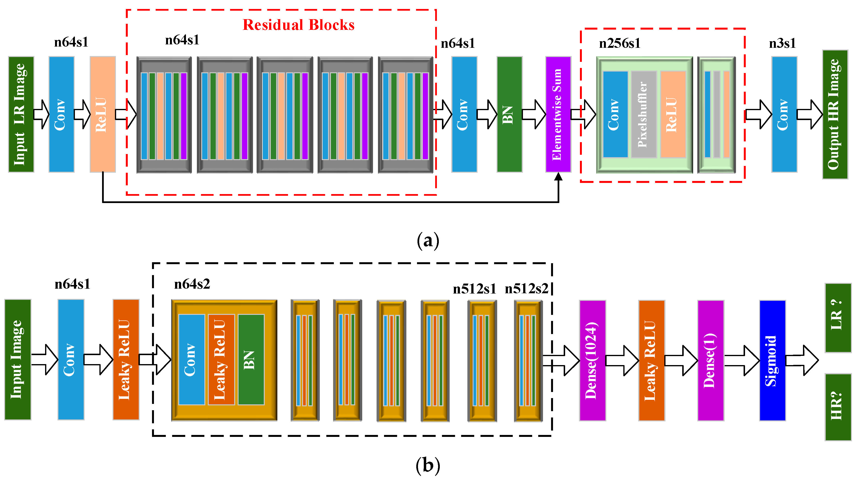
33] improved GAN to obtain super-resolution GAN (SRGAN) by replacing the loss function based on mean square error (MSE) with the the loss function of the feature map of visual geometry group (VGG) network. Under the condition of high magnification, the reconstruction of optical image from low-resolution to high-resolution was realized, and better visual effects were obtained.
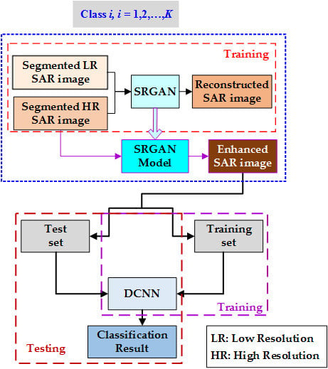
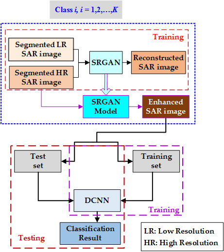
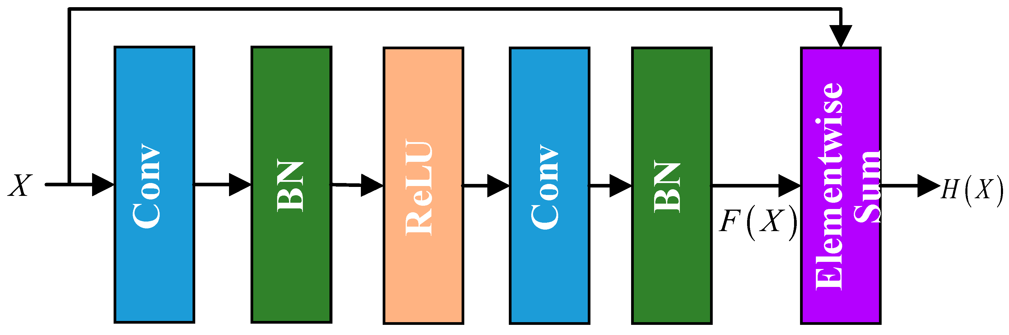
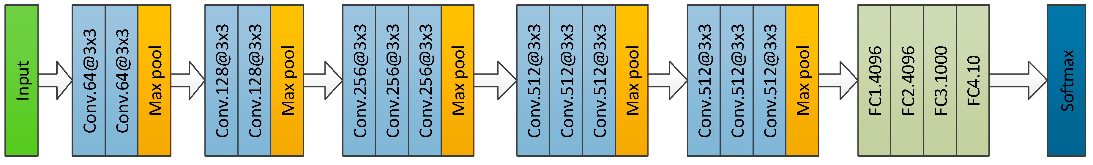
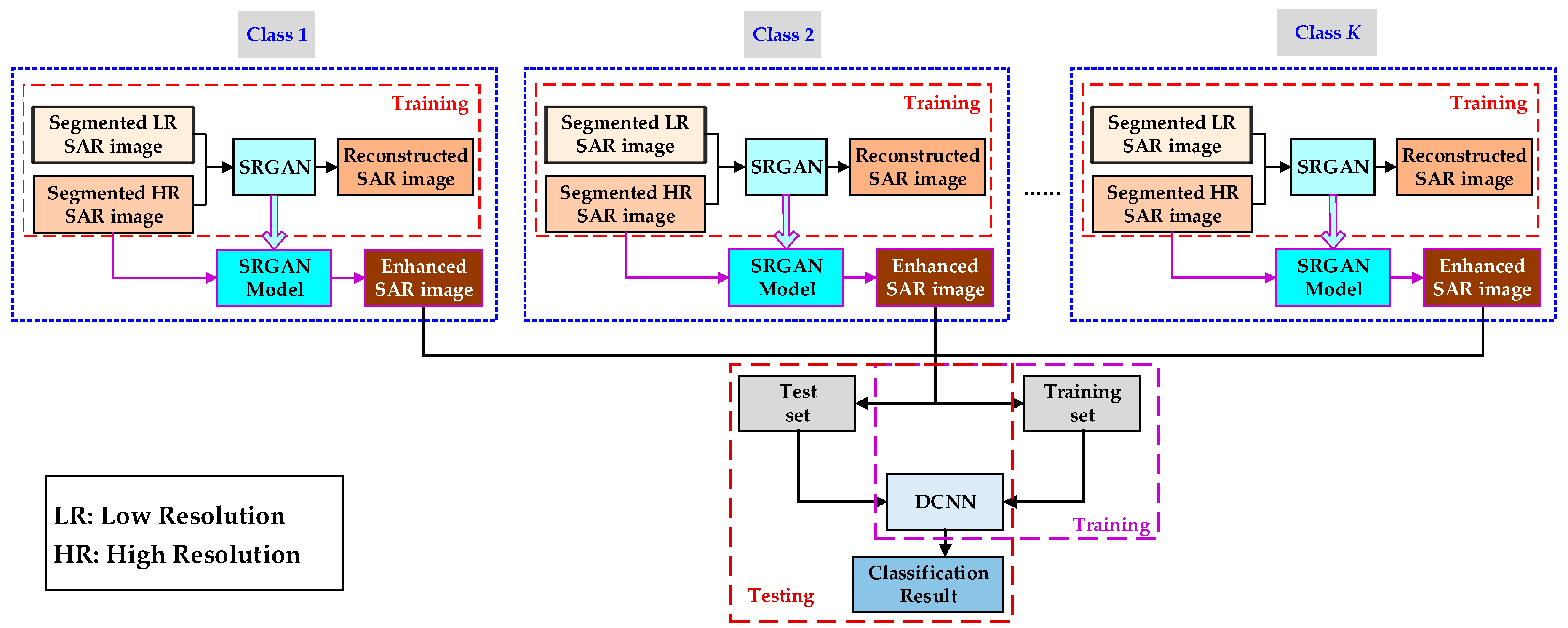
In this paper, a ATR for SAR image based on SRGAN and DCNN is proposed. First, a SAR image preprocessing method based on threshold segmentation is utilized to eliminate the influence of image background on target classification and recognition and extract effective target areas. Second, the SRGAN model is obtained through training to enhance the low-resolution SAR image, improve the visual resolution of the target areas of interest in the SAR image, and improve the feature characterization ability. Finally, DCNN with good generalization is adopted to learn the SAR target’s amplitude, contour, texture, and space information, and achieve the SAR images target classification and recognition.
The remainder of this paper is organized as follows. Section 2 describes the SAR image preprocessing method based on threshold segmentation and extracts the interested target regions. The architectures of SRGAN’s generator and discriminator and the composition of loss function are introduced in Section 3. The expression ability of the target features is improved through SRGAN. In Section 4, the basic modules of DCNN are introduced in detail, which is utilized for feature extraction and classification of targets. Section 5 provides detailed experimental results in various scenarios. Section 6 analyzes the computational complexity of the proposed method. Section 7 gives the conclusion.

2. SAR Image Pre-Processing

Since the target only occupies part of the SAR image, if the whole SAR image is classified as a sample, the background characteristics as a feature that matches the target will affect the recognition result, thus reducing the generalization performance of the ATR algorithm. If the image background noise is too strong, the recognition accuracy will be decreased. Therefore, it is necessary to use the image segmentation technique to pre-process the SAR images and extract target areas of interest in SAR images to improve the recognition accuracy and generalization performance.
The gray histogram of the image represents the statistical distribution of the gray values of image pixels. It arranges the gray values of image pixels in a descending or ascending order and counts the number of occurrences of each gray value. Generally speaking, the grayscale distribution of a SAR image is not uniform, and the image brightness of the same target is changeable under different scenes. If the same threshold value is used for segmentation of all the images, background speckle noise may be left in some images with a small threshold value, or the targets may be excessively segmented, the effective edge information of the targets cannot be retained, and the detailed features of the target may be lost with large threshold value. Therefore, it is necessary to carry out histogram equalization on the SAR image to make the grayscale distribute uniformly, expand the dynamic range of the pixel values, adjust the image contrast, and then select a uniform threshold for image segmentation.

2.1. Histogram Equalization of SAR Image

The purpose of histogram equalization is to find a mapping relation between the original image and the image after histogram equalization, thus achieving the uniform distribution of the grayscale of the transformed image [34]. Set r be the grayscale of the original SAR image and s is the grayscale of the image after histogram equalization. The transformation function from r to s can be expressed using:
s = T ( r )
where T ( ) is the transformation function. To facilitate discussion, set 0 r 1 , T ( ) needs to satisfy the following conditions:
(i)
When 0 r 1 , 0 s 1 ;
(ii)
When 0 r 1 , T ( r ) is a monotonically increasing function.
Then, the transformation function from s to r can be written as:
r = T 1 ( s )
where T 1 ( ) is the inverse transformation operator.
In order to satisfy the above conditions (i) and (ii), suppose that T ( r ) is the probability distribution function of r :
s = T ( r ) = 0 r p r ( v ) d v
Then:
d s d r = dT ( r ) d r = p r ( r )
The probability density of the transformed grayscale s can be obtained according to the probability density of the random variable function:
p s ( s ) = [ p r ( r ) d r d s ] r = T 1 ( s ) = [ p r ( r ) 1 d s / d r ] r = T 1 ( s ) = 1
It can be seen that the gray value of SAR image after transformation is evenly distributed.
For the discrete function, the accumulative distribution operator of each grayscale of histogram can be regarded as the transformation function, and the gray value of the transformed image can be written as:
q ( i ) = k = 0 i p r ( r k ) = k = 0 i n k n
where i = 0 , 1 , 2 , , 255 , n is the number of the image elements, n k is the number of elements of the grayscale r k , and p ( r k ) is the probability of the k - th grayscale.
Then, the gray value of the transformed SAR image is transformed into the range of [0, 255] according to:
s ( i ) = 255 q ( i )
It can be seen that the grayscale distribution of SAR image after histogram equalization is close to uniform distribution, and the image contrast is adjusted, which lays a foundation for the following uniform threshold selection in image segmentation.

2.2. Threshold Segmentation

SAR images are normalized after the histogram equalization, and the target regions of interest in SAR images are extracted by selecting uniform thresholds. Suppose that Q is the SAR image after equilibrium normalization, ( x , y ) is any pixel of the image Q , and P is the SAR binary mask image after threshold segmentation. If Q ( x , y ) < η , then P ( x , y ) = 0 and this pixel is regarded as the background; if Q ( x , y ) η , then P ( x , y ) = 1 and this pixel is recognized as the target. η is the uniform threshold.

2.3. Morphological Filtering

To reduce the speckle noise and unsmoothness of the target edge in the SAR binary mask image, some filtering operations are needed to smooth and suppress speckle noise. Morphological filtering is utilized here. Set B ( x , y ) be the structural element, corrosion and expansion can be defined respectively as [35]:
( Q Θ B ) ( x , y ) = min { Q ( x m , y n ) B ( x , y ) , ( x , y ) D B }
( Q B ) ( x , y ) = max { Q ( x m , y n ) + B ( x , y ) , ( x , y ) D B }
where D B is the image region corresponding to the structural element B ( x , y ) . If the size of D B is M × N , then 1 m M , 1 n N . Open and closed operations can be defined respectively as:
Q B = ( G Θ B ) B
G B = ( G B ) Θ B
Open operations can remove isolated points and burrs. Closed operations can fill the small holes in the body, close the small cracks, connect the adjacent objects, and smooth the boundary.
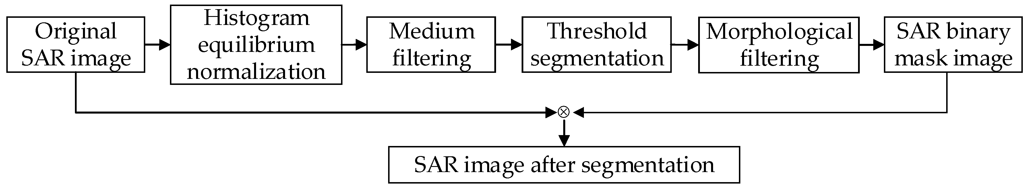
Figure 1 is the flow chart of the SAR image preprocessing using the threshold segmentation method. First, histogram equalization and normalization are adopted to the original SAR image to make the image grayscale distribution close to the uniform distribution. Then use the median filtering to smooth the normalized image. Second, select an appropriate threshold to make the SAR image binary and segment the SAR image background and the target of interest. Third, in order to solve the problem of speckle noise and burrs on the edge of the target in binary images, the closed operation of morphological filtering is utilized to obtain the SAR binary mask image. Finally, the original SAR image is multiplied by the SAR binary mask image to obtain the segmented SAR image.

3. SAR Image Enhancement Based on SRGAN

Due to the high cost for high-resolution SAR image acquisition and the poor feature characterization ability of low-resolution SAR image, it is difficult to obtain ideal results using the original image to target classification problem directly. This paper applies the technique of the SRGAN into the problem of low-resolution SAR image enhancement. Through the study of confrontation between the generator and discriminator, SAR image of high visual resolution is obtained and the capacity of the characteristics of the original SAR image feature is enhanced. Then the enhanced SAR image is sent into a classifier for classification to improve the accuracy of target recognition.

3.1. Structure of SRGAN

SRGAN is a GAN-based network optimized for a new perceptual loss by introducing the idea of super-resolution. The idea of a GAN comes from Nash equilibrium in game theory, which consists of a generator and a discriminator and predicts the potential distribution of real images and generates new images through the iterative advertised learning between them. The training and learning purpose of the generator is to generate realistic images as much as possible to cheat the discriminator, while the discriminator is to distinguish real images from false images generated by the generator as much as possible. They finally reach the state of Nash equilibrium. At last, the generator produces false images enough to confuse the human eyes, and the discriminator is also difficult to distinguish real images and false images [31].
Traditional super-resolution problems generally consider small magnification. The cost function of the traditional method is generally based on the MSE, which makes the reconstructed result have a higher signal to noise ratio (SNR). When the image magnification is above 4, the reconstructed image will lack high frequency information, appear to have an overly smooth texture, and lose some sense of authenticity in details. The training process of SRGAN is still a dynamic game process. The inputs of GAN are real samples and noise, while the inputs of SRGAN are original SAR images and low-resolution SAR images [33]. At the same time, the loss function of SRGAN contains not only the anti-loss of GAN but also content loss, which increases the similarity between the reconstructed SAR image and the original segmented SAR image in the feature space.
The architecture of SRGAN is shown in Figure 2. The generator contains five residual block subnetworks with the same structure. The number of convolutional kernels is 64, the size is 3 × 3, after which, the BN layer and the rectified linear unit (ReLU) nonlinear activation layer are connected. The ReLU is a piecewise function:
σ ( x ) = max { 0 , x }
The schematic diagram of a residual block is shown in Figure 3. It contains two convolutional layers and two BN layers and one ReLU activation layer. From Figure 3, the residual network connects the input X and the output node F ( X ) through the structure of skip mapping. It transforms the optimization function into the residual function:
F ( X ) = H ( X ) X
where H ( X ) is the expected output. At this point, we only need that F ( X ) approaches to zero to get an identical mapping, which greatly reduces the difficulty of training and it is easy to achieve network optimization. The addition of residual blocks solves the problem of network saturation degradation when the network structure is deepened [36].
After the residual block structure, two PixelShuffler layers are connected to realize upper sampling of low-resolution SAR images and the reconstruction of original segmented SAR images. SRGAN improves the SAR image resolution at the last layer, which greatly saves the computing time and memory [26].
The discriminator contains eight convolutional layers and two fully connected layers. Finally, a sigmoid function is used to activate the discriminator. Its structure is similar to that of VGG network, except that the activation function of convolutional layer is a leaky ReLU function, and basic modules of VGG network will be introduced in detail in Section 4.

3.2. Loss Functions of SRGAN

In order to represent the improvement of visual resolution, the perceptual loss function l SR is defined in SRGAN, whose expression can be written as:
l SR = l Cont SR + 10 3 l Gen SR
where l Cont SR is the content loss, and l Gen SR is the adversarial loss.
Content loss reflects the difference between the input of the low-resolution SAR image and the output of the reconstructed SAR image produced by the generator. The content loss function l X SR based on MSE can be expressed as:
l Cont SR = 1 a 2 W H x = 1 a W y = 1 a H [ I x , y HR G θ G ( I LR ) x , y ] 2
where a is the time of upper sampling; W and H represents the dimensions of the low-resolution SAR image; I x , y HR is the pixel value of the original segmented SAR image, which is the input as high-resolution SAR image at the point ( x , y ) ; I LR is the low-resolution SAR image, which is the down sampling image; and G θ G ( I LR ) x , y is the pixel value of the reconstructed high visual resolution SAR image generated according to the low-resolution SAR image I LR and the high-resolution image I HR at the pixel point ( x , y ) .
The adversarial loss function l Gen SR can be expressed as:
l Gen SR = n = 1 N log D θ D [ G θ G ( I LR ) ]
where D θ D [ G θ G ( I LR ) ] represents the probability that the discriminator regards the image generated by the generator G θ G ( I LR ) as the high-resolution image I HR .
The training process of SRGAN can be summarized as the optimization problem of network parameter θ ^ G :
θ ^ G = arg min 1 N n = 1 N l SR ( G θ G ( I n LR ) , I n HR )
where I n LR and I n HR are the n - th low-resolution SAR image and the n - th high-resolution SAR image, G θ G is the discriminant model, and N is the number of SAR images in the training set.
After the network converges, input the high-resolution SAR image as the low-resolution SAR image into the trained SRGAN model to improve the visual resolution of the high-resolution SAR image further, make the target texture clearer, enhance the feature expression ability of the image, and improve the accuracy of SAR target recognition. The original segmented image is input to the SRGAN twice. It is inputted to the SRGAN as the high-resolution SAR image for the first time in the process of training, which is utilized for the low-resolution SAR image to learn the high frequency information, detailed edge information, and the precise texture of the high-resolution SAR image. While it is inputted to the SRGAN as the SAR image to be enhanced for the second time in the process of testing.

4. SAR Image Classification Based on DCNN

The image classification method based on deep learning can automatically learn the spatial information and texture characteristics of images to avoid the intricacies of manual feature extraction and feature selection, reduce the influence of subjective factors on the classification results, and improve the universality of the classification algorithm. The most common method is CNN. Generally speaking, the accuracy of target classification can be improved by deepening the network properly. As is known, less layers means faster training. However, the CNN with less layers cannot be compared with DCNN in terms of the recognition accuracy. VGGNet is a typical DCNN developed by the University of Oxford visual geometry group and researchers at Google DeepMind. VGGNet explored the relationship between the deepness and the performance of the CNN. Through stacking the small convolutional kernels of 3 × 3 and maximum pooling layers of 2 × 2 repeatedly, VGGNet successfully constructs the CNN with 16 and 19 layers, which are called VGG16 and VGG19, respectively. VGGNet won the second class prize in classification project and the first class prize in the positioning project of the ILSVTC 2014 competition [37]. VGGNet is one classic DCNN structure with good generalization. Its structure diagram is shown in Figure 4, which is mainly composed of 13 convolutional layers, 5 pooling layers, and 4 full connection layers [38]. We have added one full connection layer based on the VGG16. The following parts give the detailed description of VGGNet.
SAR images need to be pre-processed before training and testing. According to the experience, we take the original image minus its mean as input to conduct training and testing in order to improve the stability of training and testing.

4.1. Forward Propagation

4.1.1. Convolutional Layer

The convolutional layer is a key layer for feature extraction. It extracts features by convolving the feature map of the output with the previous layer. In the process of network training, the convolutional kernel is updated continuously through the learning of feature maps. If different convolutional kernels are used for each convolution operation, with the deepening of network layers, more and more parameters need to be trained. In order to reduce the number of the training parameters of the network, CNN adopts the weight-sharing operation. In the VGGNet, the convolutional kernel is set to 3 × 3. Convolutional layer operations include convolution and activation, and the convolution process can be expressed as:
z j ( l ) = i q i ( l 1 ) ( x , y ) w i j ( l ) ( x , y ) + b j ( l ) = i m , n = 0 F q j ( l 1 ) ( m , n ) w i j ( l ) ( x m , y n ) + b j ( l )
where ( x , y ) is any pixel of a SAR image, q i ( l ) is the i - th feature map of the l - th layer, w i j ( l ) is the convolutional kernel connecting the i - th input feature map to the j - th output feature map on the l - th layer, F is the size of the convolutional kernel, b j ( l ) is the j - th bias of the l - th layer, and denotes the 2-D convolution operation. In order to increase the nonlinear characteristic of the network and make the model have stronger classification expression ability, each convolutional layer needs to connect the nonlinear activation function layer:
q j ( l ) ( x , y ) = σ ( z j ( l ) )
where σ is the nonlinear activation function ReLU. When mapped to a higher dimensional space, the final decision surface is decomposed into multiple planes. As the neural network deepens, multiple piecewise planes are required to fit the final decision surface and realize nonlinear classification. Convolutional kernels and bias are the parameters to be trained.

4.1.2. Pooling Layer

In order to reduce the number of the training parameters, the pooling layer is added after the convolutional layer to realize the “compression” of the information in the local field of vision. Pooling is divided into maximum and average pooling. Maximum pooling returns the maximum value in the pooled window, while average pooling returns the average value in the pooled window. Here, we use the maximum pooling:
q j ( l ) ( x , y ) = max m , n = 0 , , P 1 q j ( l ) ( x + m , y + n )
where P is the size of pooling window.
After several convolutional and pooling layers, the features of the image are extracted and learned.

4.1.3. Activation Function

The softmax activation layer is the last layer of the entire network, mainly completing the classification task, and its output is the posterior probability of each class of sample:
p ( y i | q ( L ) ) = exp ( q i ( L ) ) j = 1 K exp ( q j ( L ) )
where y i denotes the predicted label of the i - th class; q ( L ) is the input of the softmax layer, and it is computed by the previous fully connected layer; q i ( L ) is the weight sum of the i - th node of the output of the last fully connected layer; K is the number of class; and L is the number of the layer.
Through the softmax function, the output of the model is normalized into a probability vector, and the label corresponding to the maximum of posteriori probability is the predicted class of this sample.

4.1.4. Loss Function

After forward propagation, some rules are needed to update the network parameters. The common loss functions contain the MSE and cross-entropy loss functions. Compared with the MSE function, the cross-entropy loss function can better reflect similarity of training sample and model distribution:
L ( W , b ) = i = 1 K y ( i ) log p ( y i | q ( L ) ; W , b )
where W and b are weight sets and bias sets of all the layers in DCNN respectively, and y ( i ) is the real label of the i - th class.
The cross-entropy loss function measures the difference between the real and the predicted labels. The training process of network can be summarized as the optimization problem of the minimizing loss function.

4.2. Back Propagation

The output layer results are the predicted results of the network. The error term of the network output layer can be obtained through comparing the predicted results with the real results:
δ i L = [ y ( i ) p ( y i | q ( L ) ) ]
If the ( l + 1 ) - th layer is a convolutional layer, then the error item of the i - th feature map of the l - th layer is decided by the error item of the ( l + 1 ) - th layer and the convolutional layer:
δ i ( l ) = σ ( q i ( l ) ) j δ j ( l + 1 ) w i i ( l + 1 )
where σ ( · ) is the derivative of the ReLU activation function, and is the dot product operator.
If the ( l + 1 ) - th layer is a pooling layer, then the error item of the i - th feature map of the l - th layer can be obtained using:
δ i ( l ) = σ ( q i ( l ) ) Up ( δ j ( l + 1 ) )
where Up ( · ) represents the upper sampling operation.
According to the error term of all layers, the gradients of the weight and the bias of each layer can be calculated using:
L w j i ( l ) = q i ( l 1 ) δ j ( l )
L b j ( l ) = x , y δ j ( l ) ( x , y )
Using the gradient descent method to update the weight and bias of the network:
w w η L w
b b η L b
where η is the learning rate.
Through forward and back propagation, the network finally converges and stable network parameters are obtained. The SAR images to be tested are input to the DCNN to obtain their class attributes.

4.3. The Flow Chart of the Proposed Method

Figure 5 is the flow chart of ATR for SAR image based on SRGAN and DCNN. First, in order to obtain the corresponding low-resolution SAR image, the segmented SAR image is four-fold down-sampled. The segmented SAR image, as the high-resolution image, and the low-resolution SAR image are input into SRGAN for training. After the countermeasure between the generator and the discriminator of SRGAN, the Nash equilibrium is finally achieved and the well-trained SRGAN model is obtained. Second, the segmented SAR image as the low-resolution SAR image is input into the trained SRGAN model again to improve its visual resolution to achieve image enhancement and obtain the final enhanced SAR image. Third, the enhanced SAR image after the pre-processing of subtracting mean value is divided into a training set and a test set, where the training set is sent to the DCNN to train its network parameters and learn the intrinsic features of the SAR image until convergence. Finally, the test set is sent to the trained DCNN, and the classification results are output to achieve a good classification of the SAR targets.

5. Experiments and Results

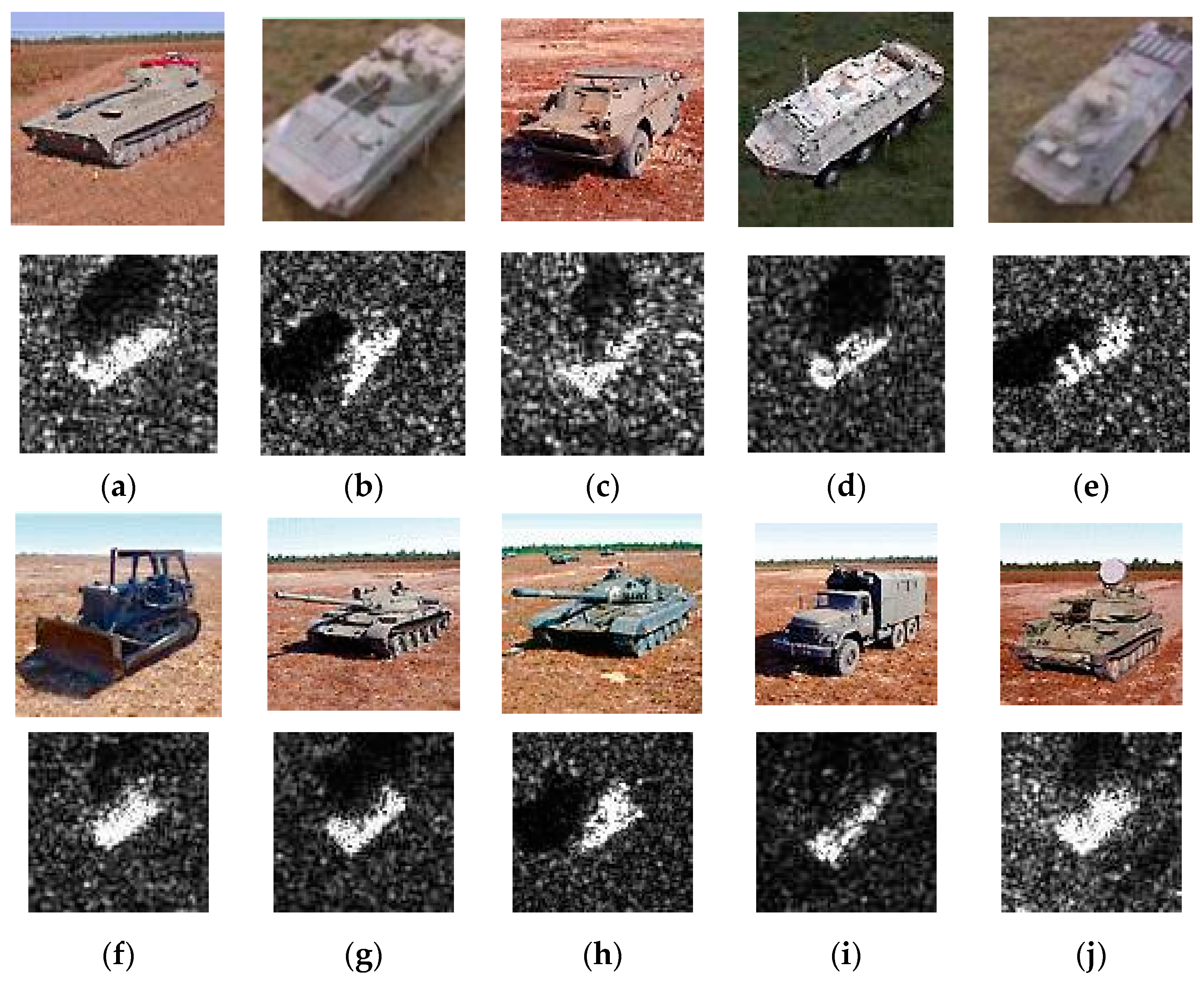
This paper utilizes the open data set, MSTAR, for the verification of the effectiveness of the proposed algorithm. The MSTAR data set was gathered in 1995 and 1996 separately by Sandia X-band (9.6 GHz) HH-polarization spotlight SAR and contains ten categories of ground military vehicles. The pitching angles were 15°, 17°, 30°, and 45°. The azimuth angles ranged from 0° to 360°. The original SAR image resolution was 0.3 m × 0.3 m and the image size was 128 × 128. These ten categories of ground military targets include BTR-70, BTR-60, BMP-2, T-72, T-62, 2S1, BRDM-2, D-7, ZIL-131, and ZSU-234. Figure 6 shows the optical images and the corresponding SAR images of the ten categories of targets. It can be seen that the resolution of SAR images is low, the targets’ edge information is not clear, and it is not easy to extract the detailed information of the images.
Experiments were conducted under SOC and EOCs [39]. SOC means that the targets of the training set and the test set have the same serial number and target configuration, but they have different azimuth and pitch angles. The differences between the training set and the test set under EOCs were large, and different controlling variables could be set such as pitch angle, configuration variant, and version variant.

5.1. SAR Image Threshold Segmentation Based on Histogram Equilibrium Normalization

Each type of target in the MSTAR data set is collected in a specific environment, and it is pointed out that these background clutter alone has an recognition accuracy of about 30% to 40% [24]. In view of this situation, the image background improves the recognition accuracy of the target to some extent. However, in the actual situation, the background of the target will vary with the specific environment. Therefore, in order to reduce the interference of the clutter of the target background on the classification results, the image needs to be segmented.
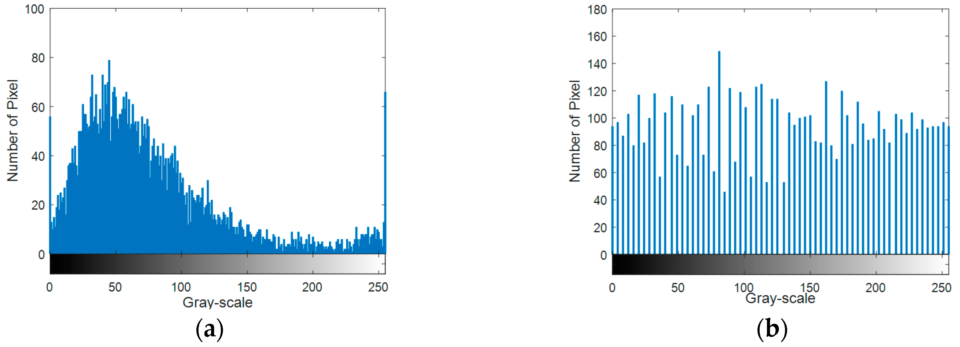
In order to facilitate the determination of the uniform segmentation threshold, first, the histogram equalization for the original SAR image was done, and then the before and after histogram results were compared, as shown in Figure 7. Figure 7a is the grayscale histogram distribution of the SAR image before equalization, and Figure 7b is the grayscale histogram distribution of the SAR image after equalization. From Figure 7, the grayscale distribution of the original SAR image was not uniform, where most of the pixels were concentrated in the range of 0 to 150, and the grayscale distribution of the SAR image after the histogram equalization was relatively even, facilitating the subsequent fixed threshold segmentation.
Taking 2S1 for example, 
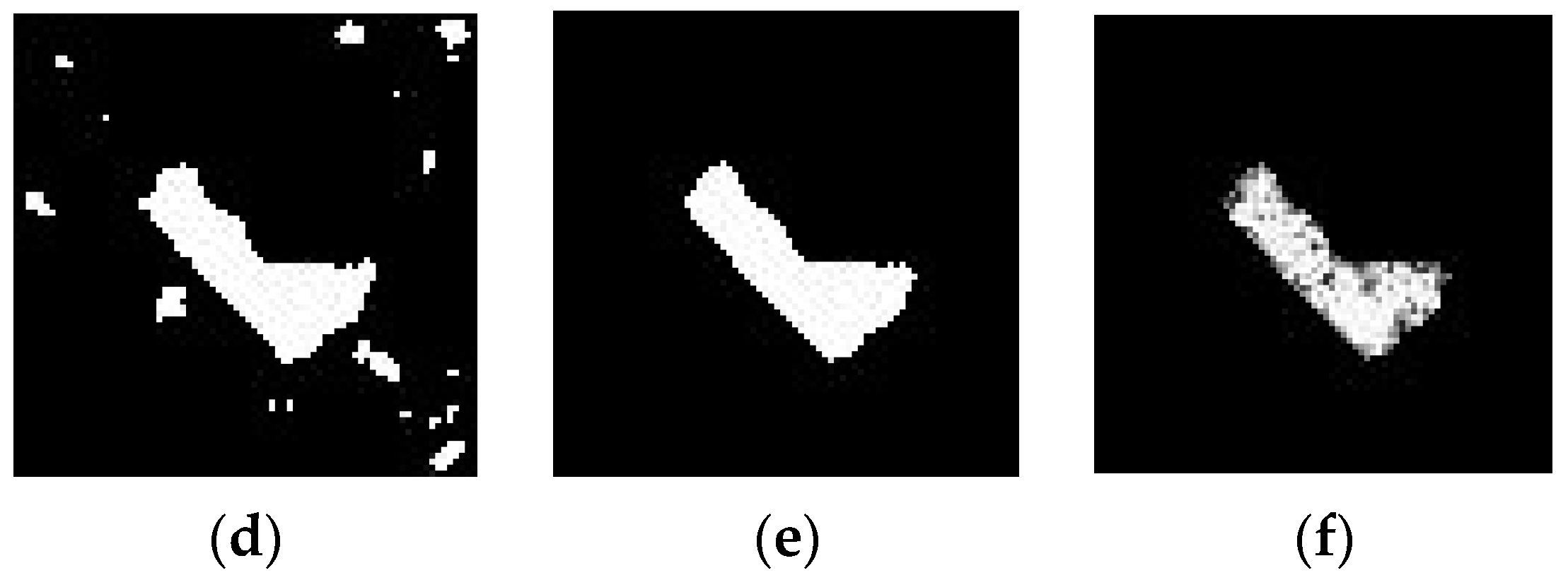
Figure 8 gives the process of the SAR image threshold segmentation. Figure 8a is the original SAR image before the histogram equalization; Figure 8b is the SAR image after equilibrium normalization, where it had a more even grayscale distribution; Figure 8c is the SAR image after median filtering, where the gray value was smoothed; Figure 8d is the SAR image after threshold segmentation, where it can be seen that there is a lot of speckle noise in the image; Figure 8e is the SAR image after morphological filtering, where the background speckle noise was well suppressed; and Figure 8f is the SAR image after segmentation, where the details and edge information of the target were well preserved.

5.2. SAR Image Enhancement Based on SRGAN

In view of the high acquisition cost of high-resolution SAR images and the inconspicuous target edge features of low-resolution SAR images, an SRGAN-based SAR image enhancement method is proposed in this paper to improve the SAR image feature characterization ability, and then the enhanced SAR image was sent to the classifier to improve the accuracy of target classification. The generator of SRGAN adds the upper sampling layer at the end to keep the image size consistent with the original image.
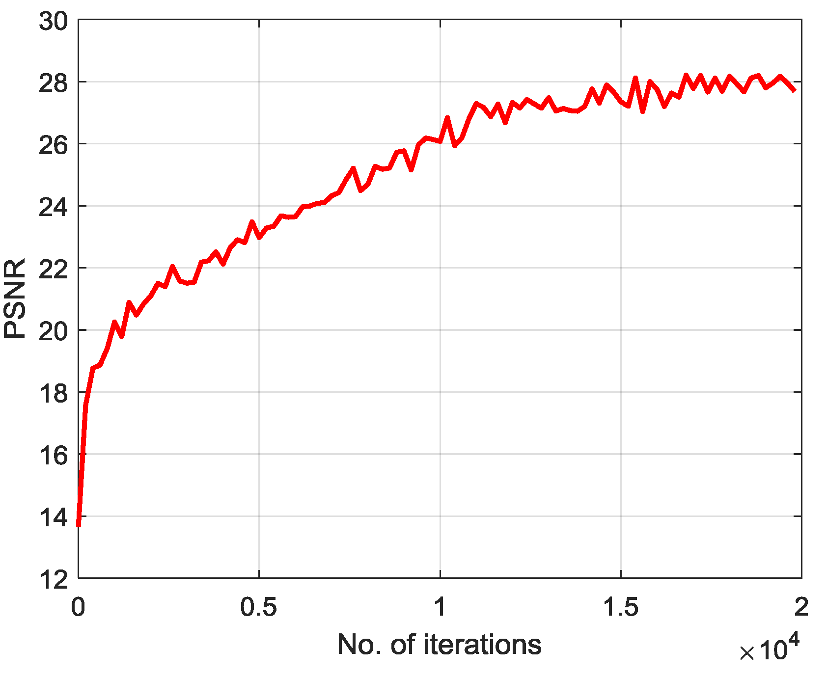
Generally, we use peak signal to noise ratio (PSNR) to measure the quality of reconstructed images. Figure 9 gives the variation curve of PSNR with number of training epoch during SAR image reconstruction based on SRGAN. From Figure 9, in the process of network training, the PSNR of the low-resolution SAR image was improved with the training epoch, and the image visual resolution is improved.
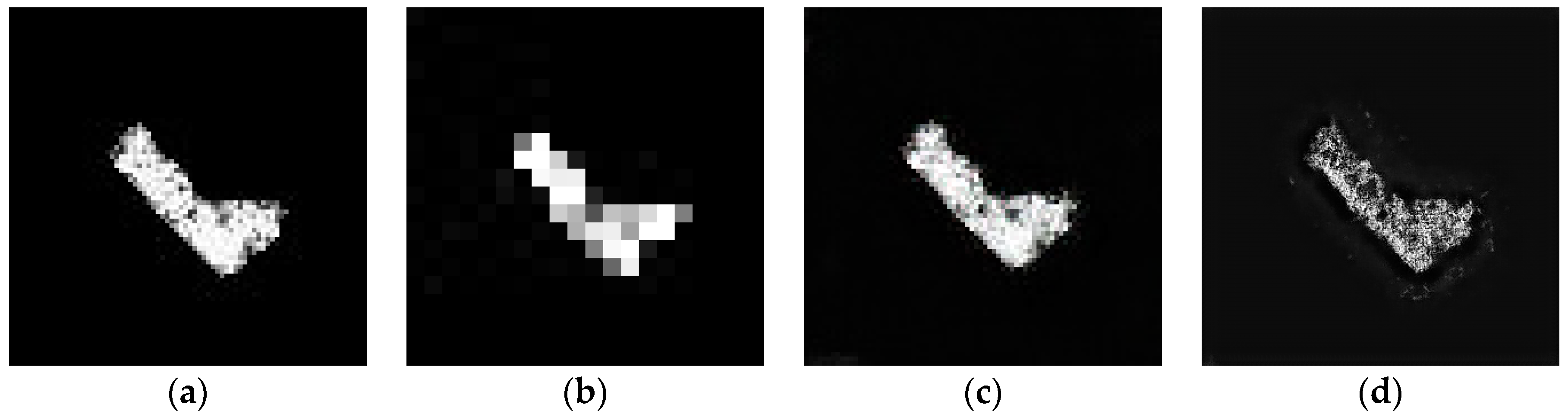
Figure 10 expresses the SAR image enhancement through SRGAN. Figure 10a shows the SAR image after segmentation, where its size was 78 × 78; Figure 10b is the low-resolution SAR image with quadruplet sampling, where the size became 19 × 19 and the image looks very blurred with a lot of information being lost; Figure 10c gives the reconstructed SAR image after SRGAN convergence, where the size was restored to 78 × 78. Compared with Figure 10a, it was very close to the original segmented image in visual sense and visual perception. It proved that SRGAN has learned the features of the original segmented image in the training process. Sending the original segmented SAR image (Figure 10a) into the trained SRGAN again, the enhanced SAR image was obtained, as shown in Figure 10d, where the size became 312 × 312. From Figure 10d, the texture information of the target surface was expressed in detail, the edge features are more obvious, and the visual resolution of the image was improved, which provides strong support for the classification and recognition of the target.

5.3. Experiments and Results under SOC

To verify the effectiveness and robustness of the proposed method, we conducted experiments in two different conditions, SOC and EOCs.
Table 1 is the description of the training set and test set under SOC. The training set contains 10 classes of targets, the pitch angles of targets in the training set were all 17°, the pitch angles of targets in the test set are all 15°. The sample numbers of each class in the training set and test set are shown in Table 1. The training set is sent into the DCNN to be trained to obtain the stable network parameters. After that, the test set is sent into the trained DCNN to obtain the final classification results.
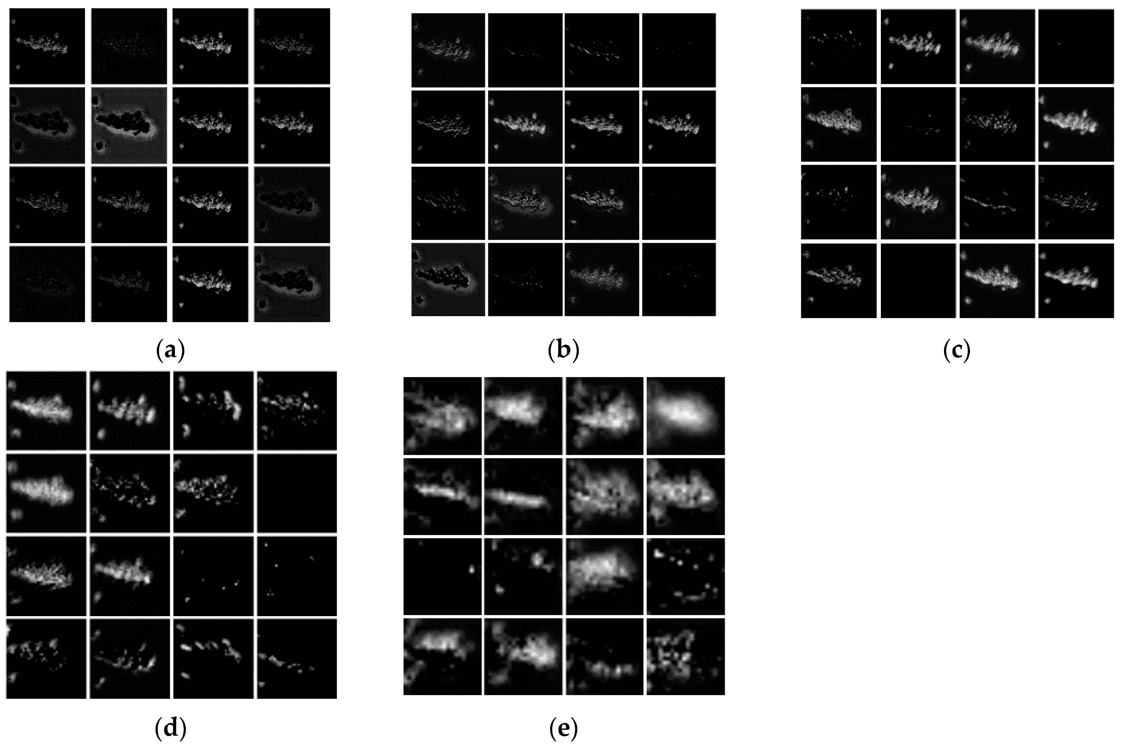
Figure 11 is the visualization result of the first 16 feature maps of five convolutional layers after sending the enhanced SAR image of 2S1 into DCNN. Figure 11a shows the feature map of the 1st convolutional layer, Figure 11b gives the feature map of the 3rd convolutional layer, Figure 11c is the feature map of the 5th convolutional layer, Figure 11d shows the feature map of the 8th convolutional layer, and Figure 11e gives the feature map of the 11th convolutional layer. From Figure 11, with the deepening of the layers, the SAR image feature characterization ability got stronger and stronger, proving that our network has learned the SAR image features.
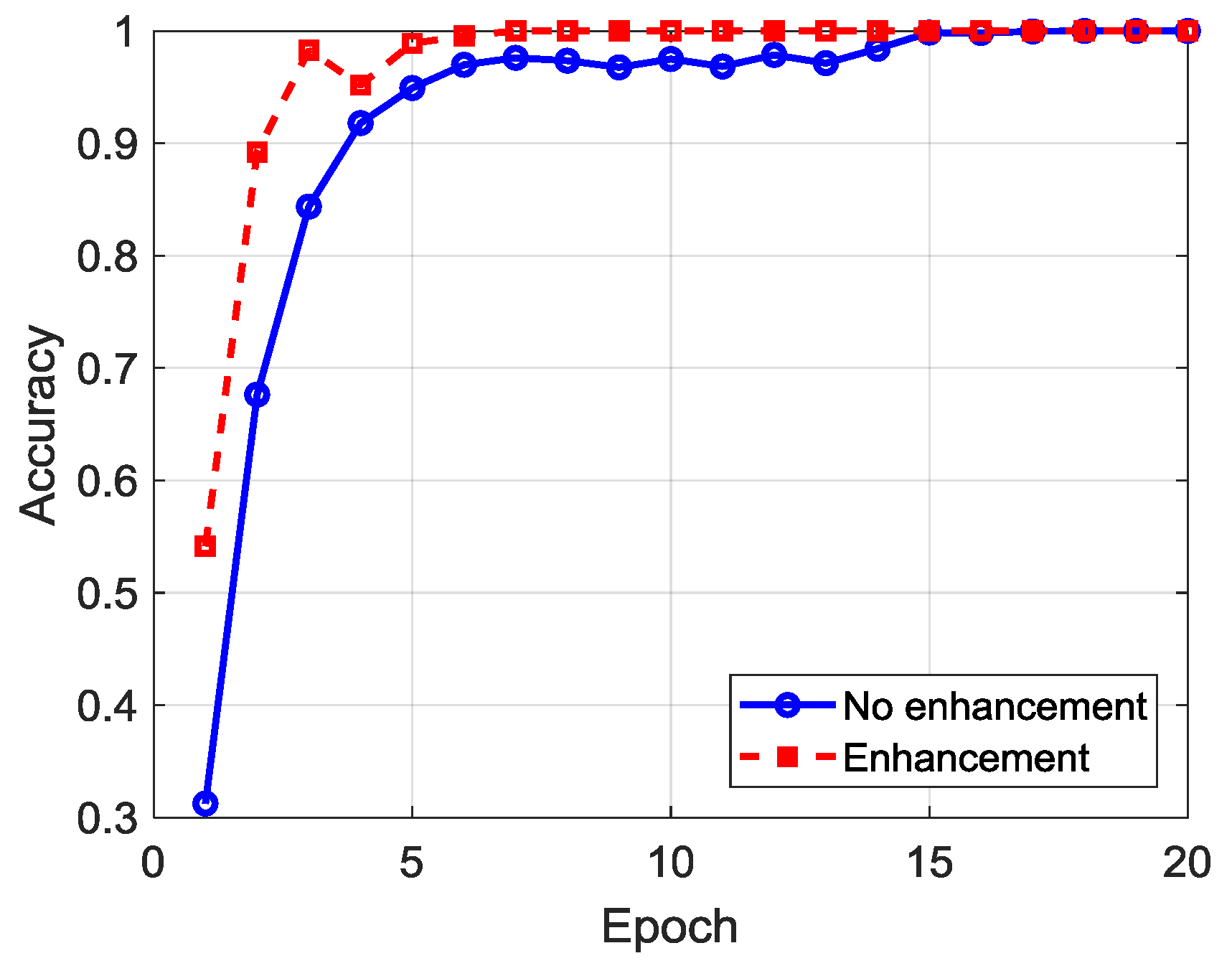
Figure 12 gives the comparison of convergence of DCNN with and without image enhancement. The solid line is the convergence curve of training accuracy with training epoch without image enhancement, and the dashed line denotes the convergence curve of training accuracy with training epoch with image enhancement. From Figure 12, the training accuracy reached a stable 100% after 15 epochs without SAR image enhancement. The convergence speed became very fast after image enhancement based on SRGAN. The training accuracy reached 100% at the fifth epoch for the first time, and it was stable after the ninth epoch. This fully proves that the features of the SAR image after enhancement were easier to extract and learn than the one without enhancement.
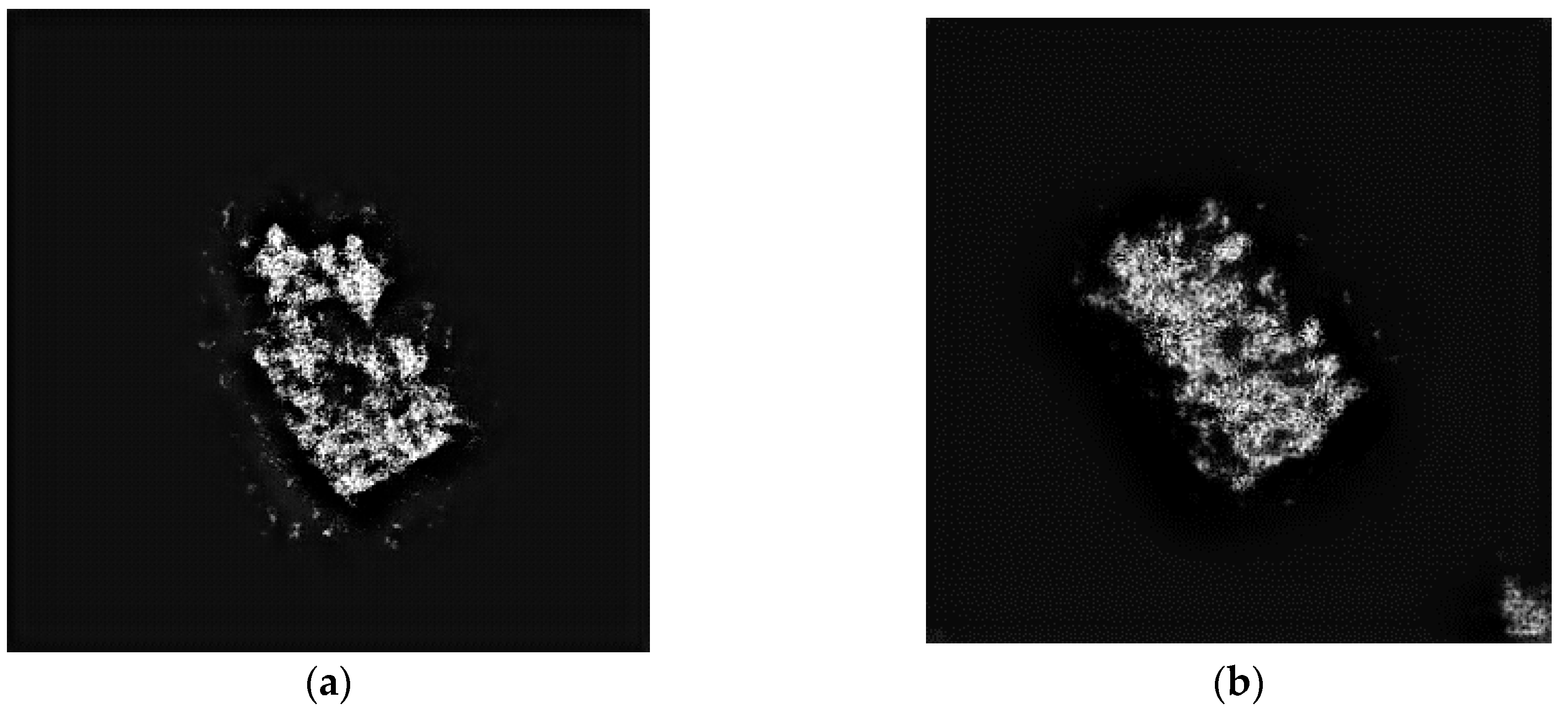
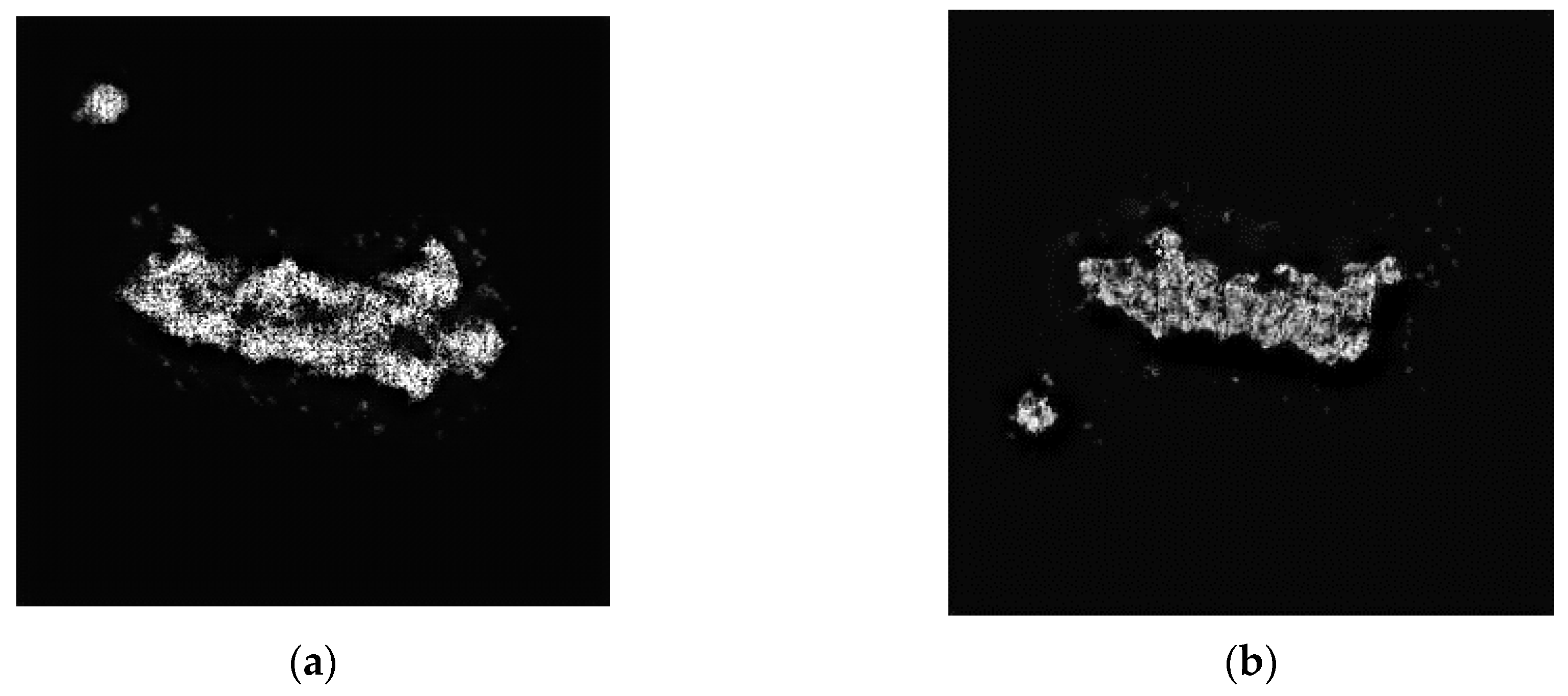
Table 2 is the confusion matrix of the recognition results of 10 classes of targets under SOC. Here, “Acc” is the abbreviation of accuracy. The SAR image average recognition accuracy of the 10 classes using the proposed method was as high as 99.31%, among which, the 2S1, BTR-70, T-72, and ZIL-131 recognition accuracy reached 100%. However, BRT-60 had the lowest recognition accuracy, which was mainly because some samples of BRT-60 were wrongly classified as ZSU-234. When the pitch angle was 17°, these two classes of target images had a great deal of similarity, as shown in Figure 13.

5.4. Experiments and Results under EOC1

For SOC, the pitch angles of the training set and the test set were different, but the difference was not large. However, the SAR image was very sensitive to many factors, and in order to verify the robustness of the method proposed in this paper, MSTAR data sets were tested in different EOCs. The EOCs need to set three different experimental conditions: different pitch angles (EOC1), and different configurations and different versions (EOC2).
There were four classes of targets in EOC1, including 2S1, BRDM-2, T-72, and ZSU-234. The number of samples of each class and the corresponding pitch angles in the training set and test set are shown in Table 3. The pitch angles of the training set and test set samples differed by 13°. The postures of the training samples and testing samples were more different than the SOC.
Table 4 is the confusion matrix under EOC1 based on the proposed method. It can be seen from Table 4, after image enhancement, that the recognition rate of each class of target was above 97%, and the average recognition accuracy reached 99.05%. Although there was a large difference of pitch angles between the training set and test set, the better recognition result under EOC1 was still obtained, which proves the robustness of the propose method.

5.5. Experiments and Results under EOC2

EOC2 is divided into different configurations and different versions. The target type, the number of samples, and the corresponding pitch angles of the training set and test set are shown in Table 5, Table 6 and Table 7, respectively. The training sets are the same for the two EOC2’s, including BMP-2, BRDM-2, BTR-70, and T-72. For the configuration variants, the test samples only included variants of T-72. For version variants, the test samples only included variants of T-72 and BMP-2.
Table 8 shows the confusion matrix under EOC2 (configuration variant) based on the proposed method. Under the configuration variant condition, the final recognition accuracy reached 99.27%, among which the T72/S7 and T72/A32 recognition accuracy reached 100%.
Table 9 is the confusion matrix under EOC2 (version variant) based on the proposed method, and the final average recognition accuracy was 98.92%. Among them, the recognition accuracy of A07 in T-72 was low, which was 96.68%. This was mainly because some T-72/A07 was wrongly classified as BRDM-2. Figure 14 gives the images of T-72/A07 and BRDM-2. It can be seen that these two classes had similarities in visual scene. There were residual regions due to the insufficient segments.
Table 10 is the comparison of different methods, namely traditional CNN, A-ConvNets, LM-BN-CNN, and the proposed method in this paper. Under SOC, the recognition accuracy of the proposed method was 4.5% higher than the traditional CNN, 4.3% higher than A-ConvNets, and 2.9% higher than LM-BN-CNN. Under EOC1, the recognition accuracy of the proposed method was 10.6% higher than the traditional CNN, 10.0% higher than A-ConvNets, and 7.4% higher than LM-BN-CNN. In the case of EOC2 (configuration variant), the recognition accuracy of the proposed method was 12.6% higher than the traditional CNN, 12.0% higher than A-ConvNets, and 10.1% higher than LM-BN-CNN. In the case of EOC2 (version variant), the recognition accuracy of the proposed method was 12.9% higher than traditional CNN, 11.8% higher than A-ConvNets, and 10.3% higher than LM-BN-CNN. It can be seen that the proposed method had stronger feature expression ability and better generalization performance, and the recognition results were superior to A-ConvNets and LM-BN-CNN. The advantages of the image enhancement are obvious, and it has better classification recognition ability when the number of target categories was fewer.
To sum up, under SOC, EOC1, and EOC2, the recognition accuracies of the proposed method in this paper were all above 98%, showing good feature expression ability and classification ability. The convergence speed of the SAR image with segmentation and enhancement was faster than the SAR image with only segmentation and without enhancement, the network was more stable, and the image features were easier to extract. There were two main reasons: First, the proposed algorithm eliminates the influence of background noise using image segmentation method and decreases the computational complexity. Second, and most importantly, the proposed algorithm adopts a super-resolution technique to improve the visual resolution of the targets in SAR images, where the detailed information becomes more obvious, such that the learning feature ability of the network is improved and the difference between different targets can be captured well, thus the recognition rate is increased. Therefore, the proposed ATR method for SAR images based on SRGAN and DCNN has effectiveness, robustness, and good generalization performance.

6. Computational Complexity Analysis

The number of parameters P of CNN is related to the depth and the number of channels of the network:
P O ( l L K l 2 C l 1 C l )
where L is the number of convolutional layer, K l is the side length of the convolution kernel of the l - th convolutional layer, and C l is the channel number of the output of the l - th convolutional layer. The number of parameters of the neural network is mainly determined by the parameters of the convolutional layer. Each neuron in the BN layer contains two trainable parameters, and the number of bias parameters of each layer contained in the convolutional layer is relatively small, meaning both can be ignored here. After the calculation, the number of parameters in the SRGAN generator was about 1.22 M, the number of parameters of the discriminator was about 4.68 M, and the total number of parameters of SRGAN was about 5.90 M. While the number of parameters of VGGNet was about 37.69 M.
The time complexity of the network is related to the network depth, the number of network channels and the size of the feature graph:
T O ( l L F l 2 K l 2 C l 1 C l )
where F l is edge length of the feature map of the l - th convolutional layer. The experiments in this paper all adopted an Ubuntu system, AMD Ryzen 7 1700X processor, with a memory of 32 GB, NVIDIA GTX1080Ti GPU, and the TensorFlow framework. The training time of each target model in SRGAN was about 17 min, the training time of classification and recognition VGGNet for 10 classes was 20 min, and the testing time of both was at the second level. Therefore, the proposed method fully meets the requirements of real-time performance and can be applied to the ELINT/EW equipment working in real conditions or other actual applications.

7. Conclusions

In view of the difficulty in obtaining high-resolution SAR image and poor feature characterization ability of low-resolution SAR image, which leads to the low SAR recognition rate, this paper proposes an ATR method for SAR images based on SRGAN and DCNN. First, the original SAR image is preprocessed by the threshold segmentation based on histogram equalization and morphological filtering to extract the target area of interest and reduce the impact of SAR image background, target shadow, and speckle noise on the recognition results. Second, the SAR image after segmentation is enhanced using SRGAN to make the texture of the target clearer and the features easier to be extracted and learned. Third, the enhanced SAR image is trained and tested by using the DCNN, and better classification results are obtained. Finally, the MSTAR data set is utilized for verification. Under the SOC and EOCs, the recognition of the proposed method in this paper was superior to the existing traditional CNN, A-ConvNets, and LM-BN-CNN, which proves the effectiveness, robustness, and good generalization performance of our proposed method.

Author Contributions

X.S. conceived and designed the experiment and analyzed the data, X.S. and S.Y. performed the experiments, X.S. wrote the paper, F.Z. and T.S. gave lots of advices, Z.Z. revised the grammar and technical error of the paper and gave lots of advices.

Funding

This paper was funded in part by the China Postdoctoral Science Foundation, grant numbers 2017M613076 and 2016M602775; in part by the National Natural Science Foundation of China, grant numbers 61801347, 61801344, 61522114, 61471284, 61571349, and 61631019; in part by the NSAF, grant number U1430123; by the Fundamental Research Funds for the Central Universities, grant numbers XJS17070, NSIY031403, and 3102017jg02014; and by the Natural Science Basic Research Plan in Shaanxi Province of China, grant number 2018JM6051.

Acknowledgments

The authors would like to thank all the anonymous reviewers and editors for their useful comments and suggestions that greatly improved this paper.

Conflicts of Interest

The authors declare no conflict of interest.

References

  1. Tang, S.; Zhang, L.; So, H. Focusing high-resolution highly-squinted airborne SAR data with maneuvers. Remote Sens. 2018, 10, 862. [Google Scholar] [CrossRef]
  2. Rahmanizadeh, A.; Amini, J. An integrated method for simulation of synthetic aperture radar (SAR) raw data in moving target detection. Remote Sens. 2017, 9, 1009. [Google Scholar] [CrossRef]
  3. Ao, D.; Wang, R.; Hu, C.; Li, Y. A sparse SAR imaging method based on multiple measurement vectors model. Remote Sens. 2017, 9, 297. [Google Scholar] [CrossRef]
  4. Dudczyk, J.; Kawalec, A. Optimizing the minimum cost flow algorithm for the phase unwrapping process in SAR radar. Bull. Pol. Acad. Sci. 2014, 62, 511–516. [Google Scholar] [CrossRef] [Green Version]
  5. Liang, Q.; Cheng, X.; Samn, S.W. New: Network-enabled electronic warfare for target recognition. IEEE Trans. Aerosp. Electron. Syst. 2010, 46, 558–568. [Google Scholar] [CrossRef]
  6. Dudczyk, J.; Wnuk, M. The utilization of unintentional radiation for identification of the radiation sources. In Proceedings of the 34th European Microwave Conference, Amsterdam, The Netherlands, 12–14 October 2004; pp. 777–780. [Google Scholar]
  7. El-Darymli, K.; Gill, E.W.; Mcguire, P.; Power, D.; Moloney, C. Automatic target recognition in synthetic aperture radar imagery: A state-of-the-art review. IEEE Access 2016, 4, 6014–6058. [Google Scholar] [CrossRef]
  8. Dudgeon, D.E.; Lacoss, R.T. An overview of automatic target recognition. Linc. Lab. J. 1993, 6, 3–10. [Google Scholar]
  9. Deng, S.; Du, L.; Li, C.; Ding, J.; Liu, H. SAR automatic target recognition based on Euclidean distance restricted autoencoder. IEEE J. Sel. Top. Appl. Earth Obs. Remote Sens. 2017, 10, 3323–3333. [Google Scholar] [CrossRef]
  10. Pei, J.; Huang, Y.; Huo, W.; Wu, J.; Yang, J.; Yang, H. SAR imagery feature extraction using 2DPCA-based two-dimensional neighborhood virtual points discriminant embedding. IEEE J. Sel. Top. Appl. Earth Obs. Remote Sens. 2016, 9, 2206–2214. [Google Scholar] [CrossRef]
  11. Dang, S.; Cui, Z.; Cao, Z.; Liu, N. SAR target recognition via incremental nonnegative matrix factorization. Remote Sens. 2018, 10, 374. [Google Scholar] [CrossRef]
  12. Novak, L.M.; Owirka, G.J.; Brower, W.S.; Weaver, A.L. The automatic target-recognition system in SAIP. Linc. Lab. J. 1997, 10, 187–202. [Google Scholar]
  13. Verly, J.G.; Delanoy, R.L.; Dudgeon, D.E. Model-based system for automatic target recognition. Proc. SPIE 1991, 1471, 266–282. [Google Scholar]
  14. He, K.; Gkioxari, G.; Dollár, P.; Girshick, R. Mask r-CNN. In Proceedings of the 2017 IEEE International Conference on Computer Vision (ICCV), Venice, Italy, 22–29 October 2017; pp. 2980–2988. [Google Scholar]
  15. Weng, C.; Yu, D.; Watanabe, S.; Juang, B.-H.F. Recurrent deep neural networks for robust speech recognition. In Proceedings of the 2014 IEEE International Conference on Acoustics, Speech and Signal Processing (ICASSP), Florence, Italy, 4–9 May 2014; pp. 5532–5536. [Google Scholar]
  16. Kolbæk, M.; Yu, D.; Tan, Z.; Jensen, J. Multitalker speech separation with utterance-level permutation invariant training of deep recurrent neural networks. IEEE/ACM Trans. Audio Speech Lang. Process. 2017, 25, 1901–1913. [Google Scholar] [CrossRef]
  17. Defense Advanced Research Projects Agency (DARPA)/Air Force Research Laboratory (AFRL). The Air Force Moving and Stationary Target Recognition Database. Available online: https://www.sdms.afrl.af.mil/index.php?collection=mstar (accessed on 10 January 2019).
  18. Zhao, Q.; Principe, J.C. Support vector machines for SAR automatic target recognition. IEEE Trans. Aerosp. Electron. Syst. 2001, 37, 643–654. [Google Scholar] [CrossRef]
  19. Wang, H.; Li, S.; Zhou, Y.; Chen, S. SAR automatic target recognition using a Roto-translational invariant wavelet-scattering convolution network. Remote Sens. 2018, 10, 501. [Google Scholar] [CrossRef]
  20. He, H.; Wang, S.; Yang, D.; Wang, S. SAR target recognition and unsupervised detection based on convolutional neural network. In Proceedings of the 2017 Chinese Automation Congress (CAC), Jinan, China, 20–22 October 2017; pp. 435–438. [Google Scholar]
  21. Chen, S.; Wang, H.; Xu, F.; Jin, Y. Target classification using the deep convolutional networks for SAR images. IEEE Trans. Geosci. Remote Sens. 2016, 54, 4806–4817. [Google Scholar] [CrossRef]
  22. Schumacher, R.; Rosenbach, K. ATR of battlefield targets by SAR-classification results using the public MSTAR dataset compared with a dataset by QINETIQ, UK. In Proceedings of the RTO SET Symposium on “Target Identification and Recognition Using RF Systems”, Oslo, Norway, 11–13 October 2004; pp. 31:1–31:12. [Google Scholar]
  23. Schumacher, R.; Schiller, J.F. Non-cooperative target identification of battlefield targets—Classification results based on SAR images. In Proceedings of the IEEE International Radar Conference, Arlington, VA, USA, 9–12 May 2005; pp. 167–172. [Google Scholar]
  24. Zhou, F.; Wang, L.; Bai, X.; Hui, Y. SAR ATR of ground vehicles based on LM-BN-CNN. IEEE Trans. Geosci. Remote Sens. 2018, 56, 7282–7293. [Google Scholar] [CrossRef]
  25. Liu, L.; Huang, W.; Wang, C.; Zhang, X.; Liu, B. SAR image super-resolution based on TV-regularization using gradient profile prior. In Proceedings of the 2016 CIE International Conference on Radar (RADAR), Guangzhou, China, 10–13 October 2016; pp. 1–4. [Google Scholar]
  26. Shi, W.; Caballero, J.; Huszár, F.; Totz, J.; Aitken, A.P.; Bishop, R.; Rueckert, D.; Wang, Z. Real-time single image and video super-resolution using an efficient sub-pixel convolutional neural network. In Proceedings of the 2016 IEEE Conference on Computer Vision and Pattern Recognition (CVPR), Las Vegas, NV, USA, 26 June–1 July 2016; pp. 1874–1883. [Google Scholar]
  27. Wang, Z.; Wang, S.; Xu, C.; Li, C.; Yue, B.; Liang, X. SAR images super-resolution via cartoon-texture image decomposition and jointly optimized regressors. In Proceedings of the 2017 IEEE International Geoscience and Remote Sensing Symposium (IGARSS), Fort Worth, TX, USA, 23–28 July 2017; pp. 1668–1671. [Google Scholar]
  28. Li, W.; Wu, Y.; Luo, D.; Zhang, H. SAR image hallucination based on Markov and Shearlet transform. J. Sichuan Univ. (Eng. Sci. Ed.) 2012, 44, 101–108. [Google Scholar]
  29. Dong, C.; Loy, C.C.; He, K.; Tang, X. Image super-resolution using deep convolutional networks. IEEE Trans. Pattern Anal. Mach. Intell. 2016, 38, 295–307. [Google Scholar] [CrossRef] [PubMed]
  30. Kim, J.; Lee, J.K.; Lee, K.M. Deeply-recursive convolutional network for image super-resolution. In Proceedings of the 2016 IEEE Conference on Computer Vision and Pattern Recognition (CVPR), Las Vegas, NV, USA, 26 June–1 July 2016; pp. 1637–1645. [Google Scholar]
  31. Goodfellow, I.J.; Pouget-Abadie, J.; Mirza, M.; Xu, B.; Warde-Farley, D.; Ozair, S.; Courville, A.; Bengio, Y. Generative adversarial nets. In Proceedings of the 27th International Conference on Neural Information Processing Systems, Montreal, QC, Canada, 8–13 December 2014; Volume 2, pp. 2672–2680. [Google Scholar]
  32. Guo, J.; Lei, B.; Ding, C.; Zhang, Y. Synthetic aperture radar image synthesis by using generative adversarial nets. IEEE Geosci. Remote Sens. Lett. 2017, 14, 1111–1115. [Google Scholar] [CrossRef]
  33. Ledig, C.; Theis, L.; Huszár, F.; Caballero, J.; Cunningham, A.; Acosta, A.; Aitken, A.; Tejani, A.; Totz, J.; Wang, Z.; et al. Photo-realistic single image super-resolution using a generative adversarial network. In Proceedings of the 2017 IEEE Conference on Computer Vision and Pattern Recognition (CVPR), Honolulu, HI, USA, 21–26 July 2017; pp. 105–114. [Google Scholar]
  34. Patel, S.; Goswami, M. Comparative analysis of histogram equalization techniques. In Proceedings of the 2014 International Conference on Contemporary Computing and Informatics (IC3I), Mysore, India, 27–29 November 2014; pp. 167–168. [Google Scholar]
  35. Wang, Q.; Wu, L.; Xu, Z.; Tang, H.; Wang, R.; Li, F. A progressive morphological filter for point cloud extracted from UAV images. In Proceedings of the 2014 IEEE Geoscience and Remote Sensing Symposium, Quebec City, QC, Canada, 13–18 July 2014; pp. 2023–2026. [Google Scholar]
  36. He, K.; Zhang, X.; Ren, S.; Sun, J. Deep residual learning for image recognition. In Proceedings of the 2016 IEEE Conference on Computer Vision and Pattern Recognition (CVPR), Las Vegas, NV, USA, 26 June–1 July 2016; pp. 770–778. [Google Scholar]
  37. Simonyan, K.; Zisserman, A. Very deep convolutional networks for large-scale image recognition. ArXiv e-prints, 2014; arXiv:1409.1556. [Google Scholar]
  38. Rumelhart, D.E.; Hinton, G.E.; Williams, R.J. Learning representations by back-propagating errors. Nature 1986, 323, 533–536. [Google Scholar] [CrossRef]
  39. Pei, J.; Huang, Y.; Huo, W.; Zhang, Y.; Yang, J.; Yeo, T.-S. SAR automatic target recognition based on multiview deep learning framework. IEEE Trans. Geosci. Remote Sens. 2018, 56, 2196–2210. [Google Scholar] [CrossRef]
Figure 1. Flow chart of SAR image preprocessing.
Remotesensing 11 00135 g001
Figure 2. Architecture of SRGAN (“n” is the no. of feature maps, “s” is the stride of each convolutional layer): (a) generator, and (b) Discriminator.
Remotesensing 11 00135 g002
Figure 3. Schematic diagram of a residual block.
Remotesensing 11 00135 g003
Figure 4. The architecture of VGGNet.
Remotesensing 11 00135 g004
Figure 5. The flow chart of ATR for SAR image based on SRGAN and DCNN.
Remotesensing 11 00135 g005
Figure 6. Ten classes of target images from MSTAR: (a) 2S1, (b) BMP-2, (c) BRDM-2, (d) BTR-60, (e) BTR-70, (f) D-7, (g) T-62, (h) T-72, (i) ZIL-131, and (j) ZSU-234.
Remotesensing 11 00135 g006
Figure 7. SAR image gray histogram distribution: (a) before the equalization, and (b) after the equalization.
Remotesensing 11 00135 g007
Figure 8. SAR image segmentation process: (a) original image, (b) equilibrium normalization, (c) medium filtering, (d) threshold segmentation, (e) morphological filtering, and (f) image after segmentation.
Remotesensing 11 00135 g008aRemotesensing 11 00135 g008b
Figure 9. The PSNR of the reconstructed SAR image.
Remotesensing 11 00135 g009
Figure 10. SAR image enhancement based on SRGAN: (a) image after segmentation (78 × 78), (b) image after quadruplet sampling (19 × 19), (c) the reconstructed image (78 × 78), and (d) the enhanced image (312 × 312).
Remotesensing 11 00135 g010
Figure 11. SAR image feature map visualization of the (a) 1st, (b) 3rd, (c) 5th, (d) 8th, and (e) 11th convolutional layer of 2S1.
Remotesensing 11 00135 g011
Figure 12. Comparison of convergence of DCNN with and without image enhancement.
Remotesensing 11 00135 g012
Figure 13. Image of (a) BTR-60 and (b) ZSU-234 in test set.
Remotesensing 11 00135 g013
Figure 14. Images of (a) T-72/A07 and (b) BRDM-2.
Remotesensing 11 00135 g014
Table 1. Description of training and test sets under SOC.
Training SetTest Set
ClassNo. of SamplesPitch AngleNo. of SamplesPitch Angle
2S129917°27415°
BMP-223317°19615°
BRDM-229817°27415°
BTR-6025617°19515°
BTR-7023317°19615°
D-729917°27415°
T-6229917°27315°
T-7223217°19615°
ZIL-13129917°27415°
ZSU-23429917°27415°
Table 2. The confusion matrix under SOC based on the proposed method.
Class2S1BMP-2BRDM-2BTR-60BTR-70D-7T-62T-72ZIL-131ZSU-234Acc (%)
2S1274000000000100
BMP-201951000000099.49
BRDM-201273000000099.64
BTR-6000118610020595.38
BTR-70000019600000100
D-700000272110099.27
T-6200000027210099.63
T-72000000019600100
ZIL-131000000002740100
ZSU-23400000100027399.64
Average 99.31
Table 3. Description of training and test sets under EOC1.
Training SetTest Set
ClassNo. of SamplesPitch AngleNo. of SamplesPitch Angle
2S129917°28830°
BRDM-229817°28730°
T-7269117°28830°
ZSU-23429917°28830°
Table 4. The confusion matrix under EOC1 based on the proposed method.
Class2S1BRDM-2T-72ZSU-234Acc (%)
2S129510298.96
BRDM-212860099.65
T-7250281097.57
ZSU-234000288100
Average 99.05
Table 5. Training set under EOC2.
ClassNo. of SamplesPitch Angle
BMP-223317°
BRDM-229817°
BTR-7023317°
T-7223217°
Table 6. Test set under EOC2 (configuration variant).
ClassNo. of SamplesPitch Angle
T-72/S741915°, 17°
T-72/A3257215°, 17°
T-72/A6257315°, 17°
T-72/A6357315°, 17°
T-72/A6457315°, 17°
Table 7. Test set under EOC2 (version variant).
ClassNo. of SamplesPitch Angle
BMP-2/956642815°, 17°
BMP-2/C2142915°, 17°
T-72/81242615°, 17°
T-72/A0457315°, 17°
T-72/A0557315°, 17°
T-72/A0757315°, 17°
T-72/A1056715°, 17°
Table 8. The confusion matrix under EOC2 (configuration variant) based on the proposed method.
ClassVariantBMP-2BRDM-2BTR-70T-72Acc (%)
T-72S7000419100
A32000572100
A6208056598.60
A63010056398.25
A6403057099.48
Average 99.27
Table 9. The confusion matrix under EOC2 (version variant) based on the proposed method.
ClassVariantBMP-2BRDM-2BTR-70T-72Acc (%)
BMP-2956642700199.77
C21429000100
T-72812000426100
A04015055897.38
A05000573100
A07118055496.68
A1008055998.59
Average 98.92
Table 10. Comparison of different methods.
MethodsSOCEOC1EOC2
(Configuration Variant)
EOC2
(Version Variant)
Traditional CNN94.7988.4486.7285.99
A-ConvNets95.0489.0587.3187.08
LM-BN-CNN96.4491.6689.1588.60
The proposed method99.3199.0599.2798.92

