High-Resolution Mass Trends of the Antarctic Ice Sheet through a Spectral Combination of Satellite Gravimetry and Radar Altimetry Observations

Abstract

Time-variable gravity measurements from the Gravity Recovery and Climate Experiment (GRACE) and GRACE-Follow On (GRACE-FO) missions and satellite altimetry measurements from CryoSat-2 enable independent mass balance estimates of the Earth’s glaciers and ice sheets. Both approaches vary in terms of their retrieval principles and signal-to-noise characteristics. GRACE/GRACE-FO recovers the gravity disturbance caused by changes in the mass of the entire ice sheet with a spatial resolution of 300 to 400 km. In contrast, CryoSat-2measures travel times of a radar signal reflected close to the ice sheet surface, allowing changes of the surface topography to be determined with about 5 km spatial resolution. Here, we present a method to combine observations from the both sensors, taking into account the different signal and noise characteristics of each satellite observation that are dependent on the spatial wavelength. We include uncertainties introduced by the processing and corrections, such as the choice of the re-tracking algorithm and the snow/ice volume density model for CryoSat-2, or the filtering of correlated errors and the correction for glacial-isostatic adjustment (GIA) for GRACE. We apply our method to the Antarctic ice sheet and the time period 2011–2017, in which GRACE and CryoSat-2 were simultaneously operational, obtaining a total ice mass loss of 178 ± 23 Gt yr⁻¹. We present a map of the rate of mass change with a spatial resolution of 40 km that is evaluable across all spatial scales, and more precise than estimates based on a single satellite mission.

1. Introduction

The Antarctic ice sheet is the largest reservoir of non-oceanic water mass. Projections estimate the ice sheet’s potential to raise sea levels by 15 m by the year 2500 for scenarios of unabated climate change [1]. It is currently in a state of overall decline [2,3], but regional differences are very prominent. Most of East Antarctica is relatively stable [4], while many glaciers in West Antarctica and the Antarctic Peninsula are losing mass due to enhanced discharge [5,6] and retreat [7] following the basal melt or structural collapse of ice shelves [8]. Some of these West Antarctic glaciers represent a serious threat to global sea levels as they could collapse within a few centuries, raising global mean sea level by centimeters to meters [9,10,11].

Satellite technology enabled much better coverage of mass balance estimates of the Antarctic and Greenland ice sheets than could be achieved with in situ or airborne measurements [2]. Three different techniques have been commonly employed to assess ice sheet mass balance: (1) The mass budget method subtracts ice discharge into the oceans and ice shelves from the net mass flux from the atmosphere onto the ice sheet’s upper surface [12]. (2) Satellite gravimetry observations (mostly by the Gravity Recovery and Climate Experiment, GRACE [13]) measure the perturbations in the gravitational potential of the Earth caused by redistribution of Earth’s mass. (3) Satellite altimetry enables repeat measurements of surface elevation, which can be used to quantify the total ice volume change and estimates of total mass change if the density at which volume changes occur can be inferred [14].

The gravimetric and altimetric approaches can both quantify the mass changes as spatial fields. However, their characteristics are very different. For example, the CryoSat-2 radar altimetry mission offers highly resolved maps of height changes [15], however, it is influenced by uncertainties from the backscattering properties of snow and firn, as well as limited resolvability of terrain with steep gradients in coastal or mountainous areas [16,17]. In addition, the conversion of volume to mass changes requires knowledge of the contributions to height changes by depositional processes which occur at the density of snow, by ice-dynamical imbalance which occurs at the density of ice, and by firn densification, which implies a height change without a mass change [18].

GRACE, on the other hand, measures mass change of the whole ice column. Although it is not affected by the presence of different processes in the snow, firn, and ice column, GRACE has a significantly lower effective spatial resolution and needs to be corrected for all other mass change processes not related to the present-day ice mass change (for example caused by short-term mass variability in the atmosphere and the ocean). GRACE mass trends need to be corrected for the Earth’s viscoelastic response to past ice changes (glacial isostatic adjustment, GIA), which is a prominent trend signal in polar regions and superimposes with the present-day mass balance (for example [19]).

Here we present a novel method to derive spatial maps of ice sheet mass change that exploits the advantages of these two techniques, while minimizing the uncertainties that are associated with each type of observation. Satellite gravimetry and laser altimetry observations of ice change have been combined before in order to separate the signals of difference processes (for example [20,21,22,23]) and also to increase the spatial resolution [24]. Here, we perform for the first time, to our knowledge, a combination in the spectral domain (i.e., in terms of the representation of the spatial fields as spherical harmonic coefficients), the common representation in which the GRACE gravity fields are estimated and distributed (Level 2 data). The combination approach can be regarded as a downward-continuation of GRACE gravity measurements to mass changes on the Earth’s surface, using mass change fields derived from CryoSat-2 data. We show that our approach allows overcoming the limited resolution of the GRACE data, producing a field of ice mass trends that is evaluable across all spatial scales, and more precise than that recovered by a single sensor. The method is applicable to other regions and components of the Earth system and may be useful to join GRACE/GRACE-FO data and additional measurements into new combined Level 4 data products.

2. Data and Methods

2.1. GRACE Satellite Gravimetry

GRACE observations of the gravitational potential are typically released by the respective processing centers as monthly sets of spherical harmonics coefficients for integer degree $j$ and order $-j \le m\le j$. Coefficients of degree $j=1$ have to be obtained from different observations (see below), the coefficient of $j=0$ is constant by definition (conservation of total mass). The spatial representation of the GRACE geoid height observation at colatitude $\theta$, longitude $\phi$, and time $t$ can be expressed as

$$g\left(\theta ,\phi ,t\right)={\displaystyle \sum }_{j=0}^{j_{\max }}{\displaystyle \sum }_{m=-j }^j\left(C_{jm}\left(t\right) Y_{jm}\left(\theta ,\phi \right)\right)$$

(1)

with $Y_{jm}\left(\theta ,\phi \right)= \{\begin{array}{c}{P}_{jm}\left(\cos \theta \right)\cos \left(m\phi \right) for m\ge 0\\ P_{j\left|m\right|}\left(\cos \theta \right)\sin \left(\left|m\right|\phi \right) for m<0\end{array}$ and $C_{j0}\equiv 0$ for $m<0$, where $P_{jm}$ is the normalized associated Legendre polynomial of degree $j$ and order $m$ [25,26]. We utilize monthly coefficients $C_{jm}\left(t\right)$ of release 5 by the Center for Space Research, The University of Texas at Austin from $j=2$ up to $j_{\max }=90$ (CSR RL05; [27]). The GRACE coefficients $\left(j,m\right)=(2$, 0$)$ are replaced by values from satellite laser ranging [28]. The GRACE spectrum is completed with coefficients of $j=1$ estimated by the approach of Swenson et al. [29]. A pole drift correction has not been applied.

We decompose the time series of each coefficient by adjusting, in a least squares sense, a temporal model consisting of the most pronounced oscillations (an annual cycle at 1 year period, the S2 tide with a 171 days repeat cycle, and the P1 tide at 161 days), as well as a linear and quadratic trend in time. For consistency with CryoSat-2 data, the adjustment period is from February 2011 to June 2017, which is the last available GRACE monthly solution. We create an ensemble of the linear trend $\frac{\partial g}{\partial t}$ by coefficient-wise random perturbation of the fitted linear trend according to the propagated standard deviation of the trend estimate (30 realizations). We subtract GIA contributions according to the three different estimates IJ05r2 [30], AGE1a [31] (this is the version independent of GRACE observations), and ICE6G [32]. Thus, we obtain 90 ensemble members representing both the uncertainties of the GRACE coefficients, as well as uncertainties of the GIA correction. Figure 1 shows the mean and standard deviation of the ensemble, as well as the uncertainty components of each ensemble as a degree-power spectrum. It is visible that the GIA-induced uncertainty peaks in the range of degree 5 to 15, while the measurement uncertainty of the coefficients gradually increases.

Note that regional optimized models exist for the Amundsen Sea Embayment [33], the Antarctic Peninsula [34], and the Siple Coast [35], yielding GIA-induced apparent mass changes of 17 Gt yr⁻¹, 3 Gt yr⁻¹, and a range of ± 6–8 Gt yr⁻¹, respectively. Using the model for the Amundsen Sea Embayment will increase the mass loss from GRACE and the discrepancy to the CryoSat-2 estimate shown later. However, these models are computed with Earth structure models optimized for these regions and should not be simply superimposed with continent-wide GIA simulations adopting an average Earth structure for Antarctica.

Each member of the geoid height trend $\frac{\partial g}{\partial t}$ ensemble is then converted to mass on the Earth surface $\frac{\partial \sigma }{\partial t}$ according to Wahr et al. [36], using load Love numbers corresponding to an elastic Earth represented by the Preliminary Reference Earth Model [37]. For clarity, we refer from now on to this surface-mass density change simply as mass change or surface load. Then, a mask is applied to the spherical harmonic spectrum using the transform method of Martinec [38] in order to reduce the far-field signal and obtain a spectral representation of the mass changes over Antarctica only. The mask is initially designed in space,$M\left(\theta ,\phi \right)$, and then analysed in terms of spherical harmonics coefficients up to $j_{\max }=90$,

$$M_{jm}= {{\displaystyle \int }}_0^{2\pi }\mathrm{d}\phi {{\displaystyle \int }}_0^{\pi }\mathrm{d}\theta \sin \theta M\left(\theta ,\phi \right) Y_{jm}\left(\theta ,\phi \right)$$

(2)

According to the relation between coefficients and the spatial function that they represent, as in Equation (1); $M\left(\theta ,\phi \right)$ is zero at any point that is more than 300 km away from the Antarctic grounding line (from Rignot et al. [39]), one at any point that is less than 200 km away from it, and linearly interpolated in between. The spectral multiplication increases the necessary degrees for the representation of the masked field to $j_{\max }=180$ [38].

Later, in the spectral combination, we will refer to the respective spherical harmonic coefficients of the $\frac{\partial \sigma }{\partial t}$ ensemble member as $C_{jm}^{\mathrm{GRACE},k}$, where $k$ specifies the ensemble member. From $C_{jm}^{\mathrm{GRACE},k}$, we calculate ensemble mean $C_{jm}^{\mathrm{GRACE}}$(indicated by the dropped superscript $k$) and ensemble standard deviation $∆C_{jm}^{\mathrm{GRACE}}$. For each degree $j$, the respective degree powers (Figure 1) are proportional to ${\displaystyle \sum }_{m=-j}^j{\left(C_{jm}^{\mathrm{GRACE}}\right)}^2$ and ${\displaystyle \sum }_{m=-j}^j{\left(∆ C_{jm}^{\mathrm{GRACE}}\right)}^2$. The magnitudes of means and standard deviations of the individual coefficients are shown in Figure 2. The spatial representations are calculated after the synthesis of the spherical harmonic spectrum of each ensemble member, as per-grid cell rates of mass change $\frac{\partial \sigma }{\partial t}$ and their respective standard deviation $\mathsf{\Delta }\frac{\partial \sigma }{\partial t}$. Unless stated otherwise, we express the mass changes in the unit ${\mathrm{kg}\mathrm{m}}^{-2}{\mathrm{yr}}^{-1}$, or equivalently in mm of the water column of density 1000 ${\mathrm{kg}\mathrm{m}}^{-3}$ referred to as mm water equivalent, per year ($\mathrm{mm}\mathrm{we} {\mathrm{yr}}^{-1}$).

Note that after isotropic filtering of the ensemble mean spatial field, the typical North-South oriented pattern of uncertainties [40] are still present in the ensemble mean, but are successfully removed by our spectral combination with CryoSat-2 observations (see Section 2.3). Our analysis shows that de-striping the gravity field observation before the combination using the filter of Swenson and Wahr [40] does not markedly change our combination results and can be omitted. Furthermore, we find that accounting for co-variances in the monthly GRACE coefficients’ using the m-block approximation [41] does not significantly alter the linear-trend estimate. We therefore adopt the variances of GRACE coefficients estimated from the post-fit residual.

2.2. CryoSat-2 Satellite Radar Altimetry

The initial measurements of the radar altimeter SIRAL on board of CryoSat-2 are radar echoes, or waveforms, from prominent reflectors in the uppermost part of the firn body, from which we eventually derive elevation rates over the period 2011–2017, following the processing scheme of Helm et al. [42], with some modifications (see Appendix A). We create an ensemble of CryoSat-2 $\frac{\partial h}{\partial t}$ estimates with the aim of representing uncertainties arising from methodical differences, as well as uncertainties from the influence of volume scatter to the elevation estimates. The ensemble consists of seven re-tracker solutions, i.e., algorithms to detect the timing of the incoming wave from the reflector, and thus elevation, as well as four least-square space-time fitting methods for aggregating the elevation measurements into linear rates of elevation change. Permutation of these processing choices gives us in total, 28 independent ensemble members. Formal measurement uncertainties are not considered in the ensemble, as our analysis indicated that uncertainties from the re-tracker and plane fitting choices are dominant. Details on the processing of the CryoSat-2 data, the re-trackers and fitting schemes are provided in the Appendix A.

For the conversion of mass changes $\frac{\partial \sigma }{\partial t}$ in the spatial domain into the spherical harmonic spectrum, all gaps in the respective height change field $\frac{\partial h}{\partial t}$ must be filled, due to the global integration over the spherical harmonic base functions (for example Equation (2)). We fill the gaps in the $\frac{\partial h}{\partial t}$ fields by interpolating using inverse distance weighting. Other, more elaborate techniques, such as kriging, are rejected here, because they are unlikely to improve the filling of the gaps, which often occur in the Antarctic Peninsula and the Transantarctic Mountains as the complex terrain distorts waveforms, and thus lets the conventional re-tracking algorithms fail [42]. Yet it is worth keeping in mind that the CryoSat-2 field is consequently less accurate in these areas. Surface elevation change outside the grounding line are set to zero, as respective floating ice changes are not visible directly in the gravity field, respectively, or the derived mass change $\frac{\partial \sigma }{\partial t}$. We do not correct for GIA in the CryoSat-2 data, as bedrock topography changes are well below 5 mm yr⁻¹ in most places [22], which is small in comparison with the measured elevation rates. Higher values have been reported in the Amundsen Sea Embayment [33], but this is also where the surface elevation rates are highest, and so the relative uncertainty remains very low. We note that the possible bias and uncertainty induced by neglecting GIA-induced crustal displacements in the CryoSat-2 only is around 9 ± 6 Gt yr⁻¹ [23].

We convert each of the above 28 realizations of CryoSat-2 surface elevation trends $\frac{\partial h}{\partial t}$ into trends of mass change $\frac{\partial \sigma }{\partial t}$, using four different assumptions on the significance of snow/ice processes, which generates a total of 112 ensemble members. Three of these methods are based on grid-based multiplying $\frac{\partial h}{\partial t}$, with the density associated with the assumed most dominant process [15,43]. The fourth method is based on the output of a regional climate model [44]. Figure 1 shows the uncertainty associated with the density models, as wells as with the re-tracker and adjustment method as a degree-power spectrum.

The CryoSat-2 fields, being available at a resolution of 5 km here, would, in principle, allow a spherical harmonic expansion to degree $j_{\max }\approx \frac{20000 km}{5 km}= 4000$. For the sake of efficiency, we opt for a maximum spherical harmonic degree of $j_{\max }=512$, equivalent to about 40 km spatial resolution in latitudinal direction, which is sufficient to demonstrate the feasibility of our approach, however, is somewhat coarser than the spatial resolutions < 32 km, adopted by many continent-wide ice sheet models [45]. We transfer the $\frac{\partial \sigma }{\partial t}$ from the grid equidistant in polar stereographic coordinates to a grid equidistant in latitude and longitude (0.2°) by bilinear interpolation to the polar stereographic projected latitude and longitude nodes. The spherical harmonics spectra of the 112 CryoSat-2 ensemble members are then generated from these re-gridded fields, according to the relation given in Equation (2). In accordance with our nomenclature for spherical harmonic coefficients of the mass change field $\frac{\partial \sigma }{\partial t}$ from GRACE, we will refer to the respective ensemble member $l$, represented by its coefficients as $C_{jm}^{\mathrm{CS}2,l}$, where superscript ‘CS2’ stands for CryoSat-2. Likewise, the ensemble mean and standard deviations are $C_{jm}^{\mathrm{CS}2}$ and $∆C_{jm}^{\mathrm{CS}2}$, respectively.

2.3. Spectral Combination

The combination of GRACE and CryoSat-2 exploits the different noise characteristics of each satellite observation that is dependent on the spatial wavelength of the mass fields. While GRACE uncertainties are known to increase with spatial resolution, due to the ill-posed and unstable nature of the gravimetric inversion problem (for example [46]), uncertainties of CryoSat-2 are expected to be sensitive to large-scale offsets or regional uncertainties in the snow/ice density necessary for the conversion from volume rates to mass rates. The GRACE coefficient at degree and order larger than 50 (spatial resolution of ca. 400 km) are typically dominated by noise, coefficients beyond degree and order ca. 90 (spatial resolution of 220 km) are often not provided in the GRACE gravity field solutions. In this sense, our combination can be interpreted as augmenting the low-frequency GRACE spherical-harmonic spectrum with higher frequencies provided by CryoSat-2, using an uncertainty weighted, optimal blending of both data sets in the spectral range j ≤ 90. From a geophysical point of view, our combination is a downward-continuation of the GRACE-measured gravitational perturbation at satellite altitude to the sources of mass change on the Earth’s surface with CryoSat-2.

For the combined spectrum of GRACE and CryoSat-2, we find weights for GRACE ($w_{jm}^{\mathrm{GRACE}}$) and CryoSat-2 ($w_{jm}^{\mathrm{CS}2}$) spherical harmonic coefficients according to the standard deviation of the ensemble for each mission in each coefficient

$$w_{jm}^{\mathrm{GRACE}|\mathrm{CS}2}=N_{jm}^i{\left(∆C_{jm}^{\mathrm{GRACE}|\mathrm{CS}2}\right)}^{-2},$$

(3)

with the normalization factor

$$N_{jm}^i={\left({\left(∆C_{jm}^{\mathrm{GRACE}}\right)}^{-2}+{\left(∆C_{jm}^{\mathrm{CS}2}\right)}^{-2}\right)}^{-1}.$$

(4)

Due to the decreasing signal-to-noise ratio in the GRACE observations with increasing degrees (for example [36]), we set the GRACE weights to zero beyond degree 90, and ensure a smooth transition within 5 degrees by the ad hoc multiplication of $∆C_{jm}^{\mathrm{GRACE}}$ by $\left(1-{\left(\frac{j-85}{5}\right)}^2\right)$ for $85\le j\le 90$ in Equations (3) and (4). For GRACE ensemble member $k$ and CryoSat-2 ensemble member $l$, the resulting coefficients of the combined field (superscript ‘Comb.’) are then given as

$$C_{jm}^{\mathrm{Comb}.,k,l}=C_{jm}^{\mathrm{GRACE},k} w_{jm}^{\mathrm{GRACE}}+C_{jm}^{\mathrm{CS}2,l} w_{jm}^{\mathrm{CS}2}.$$

(5)

This means that the weighting factors calculated from (3) are the same for all ensemble members $k$ and $l$ in the combination (5), respectively. The resulting full spectrum up to degree and order 512 (not shown) is transferred into the spatial domain (see Section 3.2) for respective ensemble mean and standard deviation. Note that due to the noise characteristics of GRACE and CryoSat-2, $w_{jm}^{\mathrm{GRACE}}$ represents a low-pass filter, while $w_{jm}^{\mathrm{CS}2}$ represents a high-pass filter, as seen by the uncertainty characteristics shown in Figure 1 and Figure 2.

2.4. Limitations of the Spectral Combination

The spectral combination makes use of complementary wavelength-dependent noise characteristics and resolution capabilities of GRACE and CryoSat-2. However, as a downside of the spectral combination, artefacts may appear if both spectral parts are not fully consistent, which is likely, as they are obtained from two observing systems sensitive to different processes. For example, Figure 1 shows lower degree-power for CryoSat-2 in spectral range j < 50 compared to GRACE, which, in our case, translates into a lower magnitude of total mass balance (see Section 3.3). This spectral difference will, in combination with GRACE, lead to an inconsistent spherical-harmonic representation of the true (unknown) mass field. Therefore, signal artefacts may appear, visible in our combined field as minor mass changes over ocean areas that were previously set to zero by masking (Section 2.1 and Section 2.2). For example, a slightly negative signal is visible in the ocean part of the Amundsen Sea Sector (see Section 3); here, the high-frequency supplied by CryoSat-2 does not cancel ocean leakage from GRACE completely. Note that similar—however, less obvious—issues arise when inconsistent gridded fields are averaged.

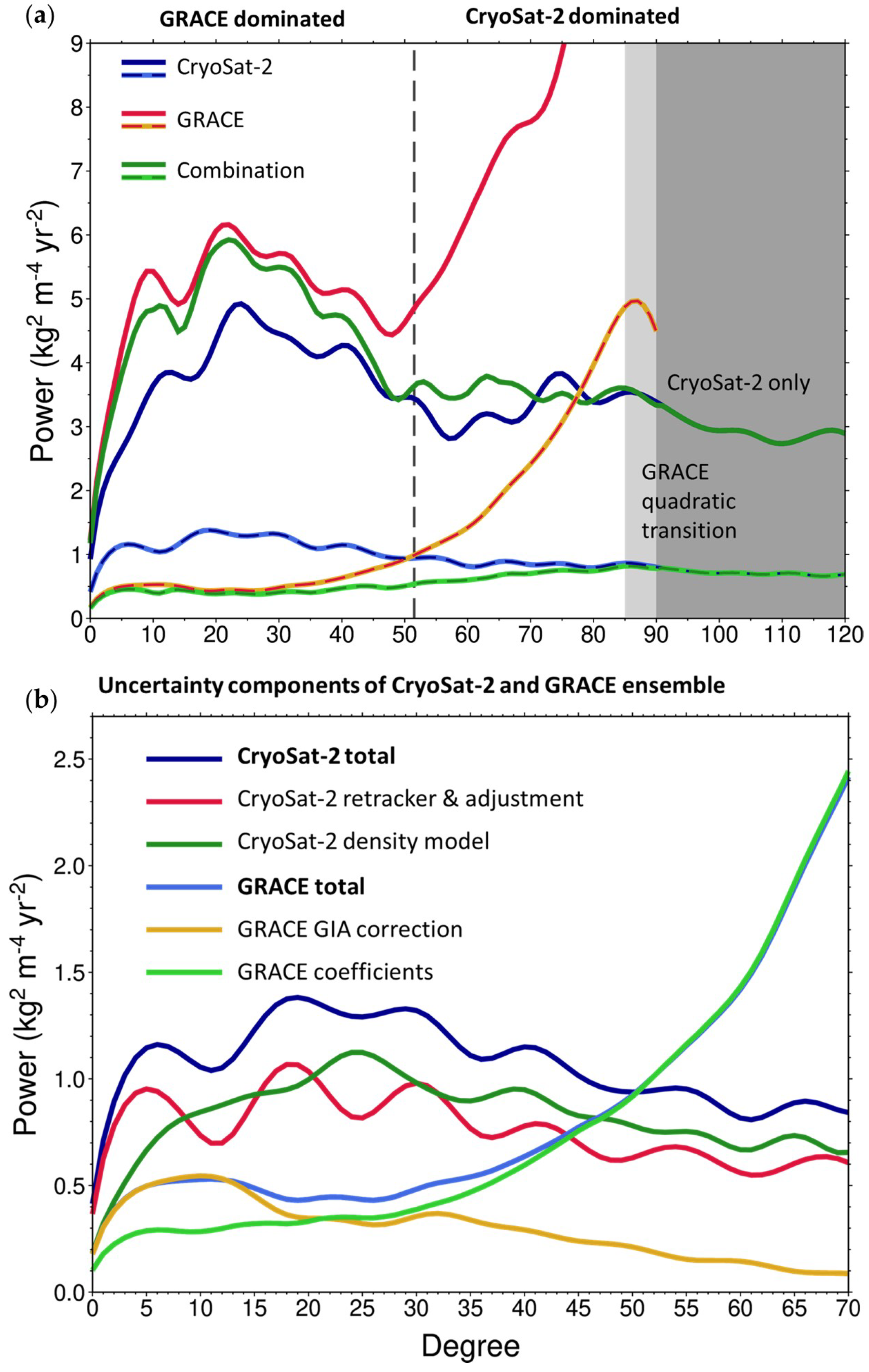
2.5. GRACE and CryoSat-2 Contributions

We quantify how much signal power GRACE and CryoSat-2 contribute to the combined field at each spatial scale, i.e., up to each harmonic degree $j$. For this, we quantify the cumulative sum of the degree power according to $p_j^{\mathrm{GRACE}|\mathrm{CS}2}\propto {\displaystyle \sum }_{j^{\prime }=0}^j{\displaystyle \sum }_{m=-j^{\prime }}^{j^{\prime }}{\left(C_{j^{\prime }m}^{\mathrm{GRACE}|\mathrm{CS}2} w_{j^{\prime }m}^{\mathrm{GRACE}|\mathrm{CS}2}\right)}^2$ and evaluate this quantity relative to the cumulative degree power of the mean combined spectrum:

$$P_j^{\mathrm{GRACE}|\mathrm{CS}2}=p_j^{\mathrm{GRACE}|\mathrm{CS}2} / \left(p_j^{\mathrm{GRACE}}+p_j^{\mathrm{CS}2}\right)$$

(6)

This choice of relating $P_j^{\mathrm{GRACE}|\mathrm{CS}2}$ to the overall cumulative power of the combined field has the advantage that $P_j^{\mathrm{GRACE}}+P_j^{\mathrm{CS}2}=100\%$, and the disadvantage that the term $p_{j^{\prime }}^{\mathrm{GRACE}}+p_{j^{\prime }}^{\mathrm{CS}2}$ does not fully represent the cumulative power of the mean combined field $p_j^{\mathrm{Comb}.}$, due to the quadratic term in the computation of degree power. However, $p_j^{\mathrm{GRACE}}+p_j^{\mathrm{CS}2}$ and the actual cumulative degree power of the mean combined spectrum $p_j^{\mathrm{Comb}.}$ differ by a maximum of ~ 6% of $p_j^{\mathrm{Comb}.}$ (reached at $j=90$), indicating that our approach is valid. In turn, this means that we can determine the optimum mix of the two sensors’ observations for a targeted spatial resolution.

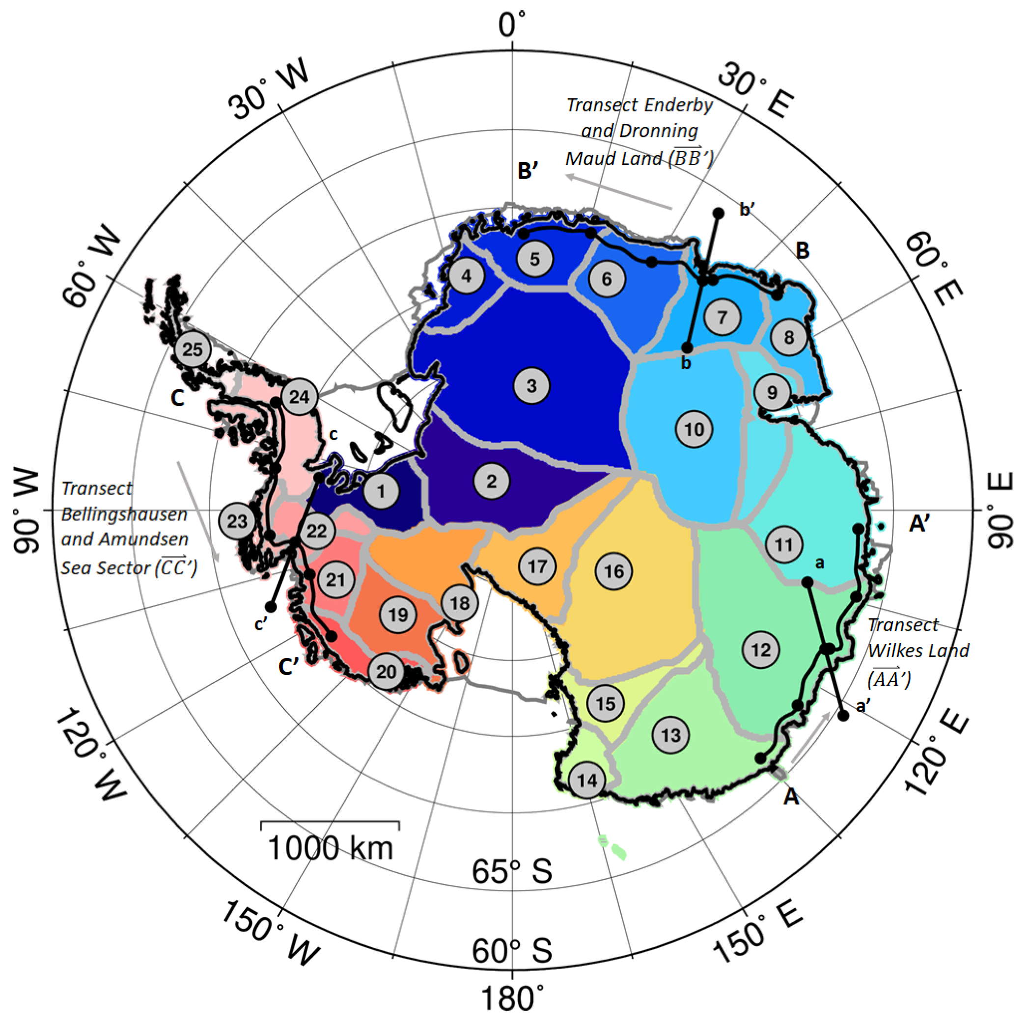
2.6. Basin Averages and Transects

For comparison with studies providing GRACE only estimates (for example [3]), we provide integrated mass balance for 25 commonly used Antarctic drainage basins, shown in Figure 3 (after Rignot et al. [12]; used in Sasgen et al. [23]). We quantify the mass balance within the basin based on the spatial representation for each $k$ (GRACE), $l$ (CryoSat-2), and $\left(k, l\right)$ (combined) ensemble member according to $m_N={\displaystyle \sum }_n\frac{\partial {\sigma }_n}{\partial t} A_n$, where $n$ indicates the running index of grid elements within a certain basins $N$, and $A_n$ is the associated area of this grid element. Based on these ensembles, we compute mean and standard deviations of the integrated basin mass balances for GRACE, CryoSat-2, and the combined solution. In the following, the uncertainties provided represent one standard deviation.

In addition, we assess the spatial resolution and decorrelation effects of our combined estimate by evaluating $\frac{\partial \sigma }{\partial t}$ and $\mathsf{\Delta }\frac{\partial \sigma }{\partial t}$ field along three 2000 km long transects, which run approximately parallel to the grounding line, however shifted inland by approximately 200 km (Figure 3). We have selected three regions of particular interest: (1) Wilkes Land, East Antarctica (transect AA’), where very localized ice dynamic imbalance has been noted at the Totten glacier system (for example [47]). (2) Dronning, Maud, and Enderby Land (transect BB’), where strong accumulation variations are observed [48]. And (3) the Amundsen Sea and Bellingshausen Sea Sectors (transect CC’), where the largest ice dynamic losses for Antarctica are recorded (for example [49]). The transects are chosen approximately across the ice-dynamic flow line to assess whether glacial entities smaller than the typical basin scale can be resolved. In addition, we assess the mass rate fields locally perpendicular to the transects described above, namely along Totten Glacier (aa’), Shirase Glacier (bb’), and Pine Island Glacier (cc’). Crossing the division between the Antarctica continent and the surrounding ocean or ice shelf areas allows us to assess the signal leakage beyond the coastline into the open ocean. Note that we do not attempt to adopt the exact grounding and flow line positions of the ice streams, which is beyond the capabilities of CryoSat-2, and thus, the combined product.

3. Results

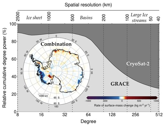
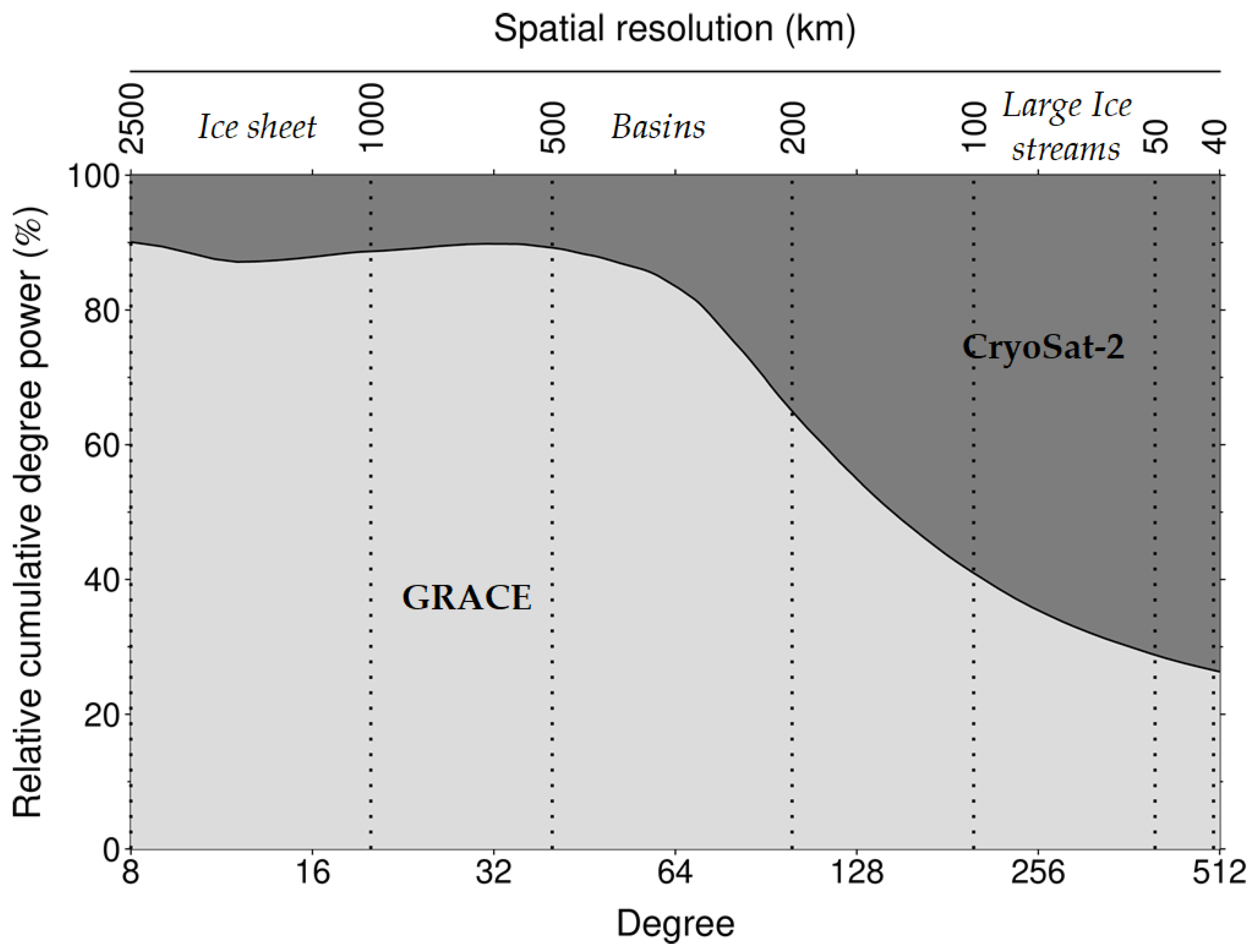
3.1. Spectral Representation

The magnitude of the coefficients of the ensemble mean and the ensemble standard deviations of CryoSat-2, GRACE, and the combined solution are shown in Figure 2 for $j\le 90$. The magnitude per coefficient is centered close to the zonal coefficients (m = 0), with lower values in the sectorial coefficients (j = m). This is a result of Antarctica’s geographical position approximately centered on the South Pole, with data coverage only south of 60°S. Note that the spectrum of CryoSat-2 is more focused towards the zonal coefficients than GRACE, owing to the mask buffer zone of 300 km adopted for GRACE (Section 2.1) and the North-South oriented noise pattern. The overall magnitude of GRACE coefficients is larger in the low degrees and orders, and noise is starting to dominate around degree and order 50.

The ensemble per-coefficient standard deviations (Figure 2, right panels) confirm the noise structure shown in Figure 1; the variability caused by the choice of the re-tracker and density model in CryoSat-2 creates uncertainties in the lower degree part of the spectrum, similar to the characteristics signal spectrum itself. For GRACE, the well-known increase of the noise with degree and order is visible, suggesting an onset of the noise dominated regime at about degree and order 60. The combined solution retains the spectral magnitude in the low degrees and orders, while reducing noise in the high degrees and orders.

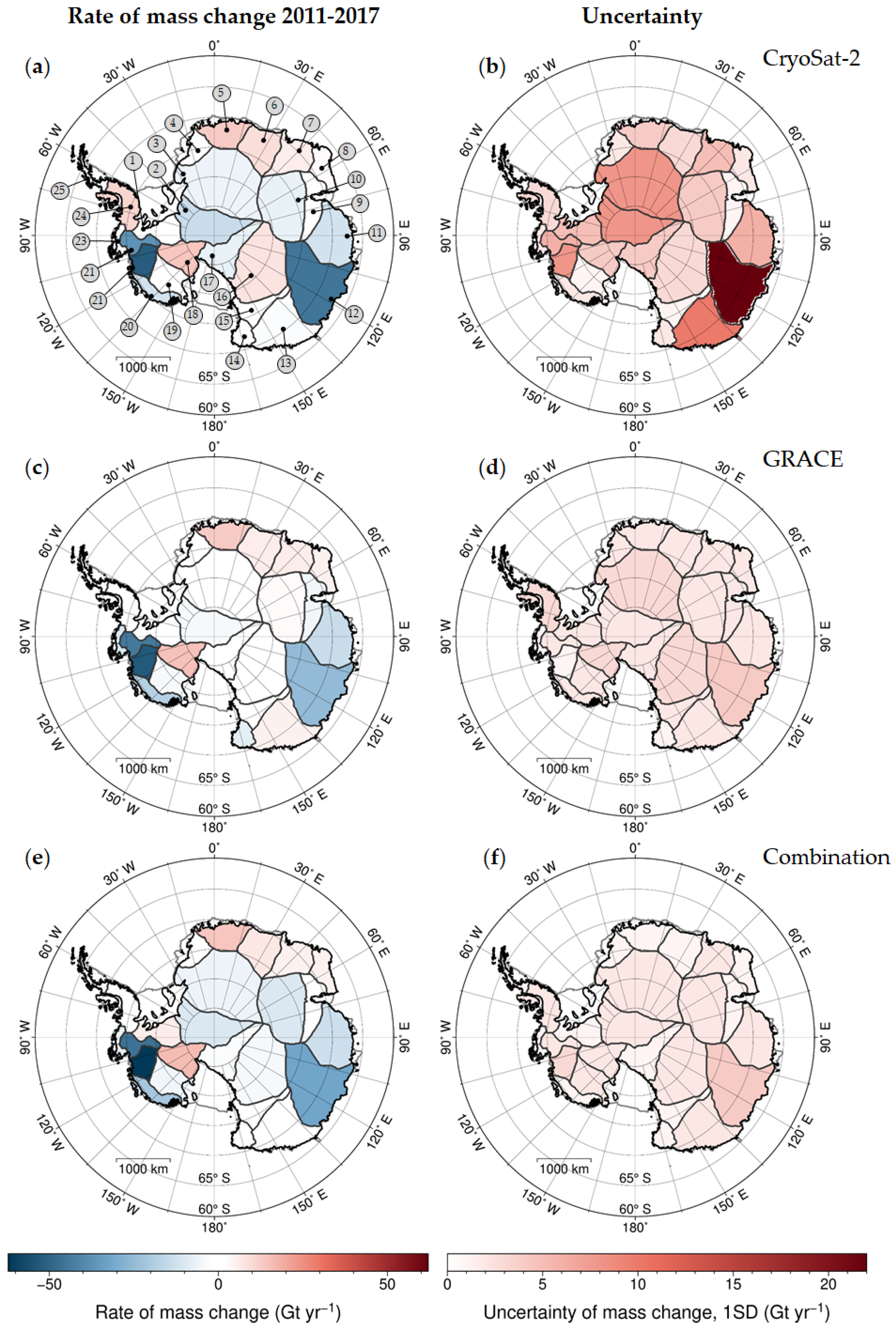
3.2. Spatial Representation

Figure 4 shows the spatial representation of the CryoSat-2, GRACE and the combined field together with their respective uncertainties. For reference, we have labeled prominent features of mass change in the spatial representation of the ensemble mean CryoSat-2 field (Figure 4). These include the well-known hotspots of ice dynamics losses in the Amundsen Sea Embayment (Figure 4, Label 1; for example [49]), the slowing of Ice Stream C (Label 2; for example [50]), and the Totten glacier system (Label 3; for example [47]). In addition, CryoSat-2 shows a large-scale, low-magnitude mass loss signal in the interior part of Wilkes Land (Label 4) and prominent accumulation driven mass gain is shown along the Antarctic Peninsula (Label 5; [6]).

The uncertainty of the CryoSat-2 ensemble mostly correlates with the signal structure, as the variability of the density models has the largest effects where the CryoSat-2 $\frac{\partial h}{\partial t}$ signal. However, in the interior of Wilkes Land (Label 4), uncertainties are induced by differences in the re-trackers due to varying backscattering properties of the snow and ice (for example [42]). Another remarkable feature in the CryoSat-2 uncertainty is CryoSat-2’s mode mask boundary south of the Filchner Ice Shelf. Note that also some Gibb artefacts (for example [51]) are present, mostly beyond the ice sheet boundaries, for example in the Amundsen Sea, caused by the representation of the ∂σ/∂t field by a finite spherical harmonic expansion and synthesis.

The GRACE ∂σ/∂t field (Figure 4) shows the prominent mass loss in the Amundsen Sea Embayment. For visualization, we present the GRACE trends after smoothing with a Gaussian filter of 1.3° (for example [36]), reducing most of the noise and revealing the mass change anomalies. The GRACE noise field is not filtered for correlated north-south striping errors. The uncertainty represented by the ensemble standard deviation shows a striped pattern, caused by the correlation of uncertainties in the GRACE coefficients, the uncertainty due to the Polar gap of ± 0.5°, as well as an uncertainty increasing with latitude towards the equator, which is due to decreasing ground track density of the GRACE near-polar orbits (for example [52]). It is worth noting that CryoSat-2 and GRACE show very different, and, to some extent, complementary patterns of the uncertainty, for example in the Amundsen Sea Embayment.

In the combined field, some important differences are visible; first, the magnitude of mass losses in the Amundsen Sea Embayment is increased with respect to CryoSat-2 only (Figure 4, Label 1), as the signal magnitude is adjusted towards GRACE based on each sensor’s uncertainty. In contrast, the magnitudes for Ice Stream C (Label 2) and Totten (Label 3) are unchanged, suggesting initial consistency between GRACE and CryoSat-2. However, the mass loss signal and its uncertainty in the interior of Wilkes Land (Label 4) is strongly reduced, mitigating the artefacts caused by the re-trackers, and possibly an overestimation of mass loss by CryoSat-2 caused by a depletion in snow. Similarly, the mass increase along the Antarctic Peninsula (Label 5) visible in CryoSat-2 is reduced by combining with GRACE. The height change in CryoSat-2 is likely caused by snow accumulation (more than is assumed in the density models), and thus detected only at lower magnitudes by GRACE. Compared to an individual sensor, the uncertainty of the combined solution (Figure 4) is considerably reduced, removing the sensor-specific patterns of regional or zonal uncertainty.

3.3. Basin Averages

Next, we evaluate the GRACE, CryoSat-2, and combined fields, as integrated over the 25 Antarctic drainage basins shown in Figure 3, which are considered independently resolvable by GRACE (for example [53,54]).

Table 1. Mass balance of 25 Antarctic drainage basins shown in Figure 3. Listed are basin area, mass balance, uncertainty of mass balance as a result of this study, as well as the mass balance from GRACE Level 3 mascon product of Center for Space Research, University of Texas (CSR RL05 M) and the gridded product of the Climate Change Initiative (CCI) of the European Space Agency (ESA). Color coding is the same for the mass balances and the uncertainties, respectively. Red colors denote rates of mass gain, blue colors rates of mass loss. The color range is mapped to the value range from zero to the largest negative and positive values, respectively.

Basin No. N	Area (104km2)	Mass Rates (Gt yr−1), This Study			Uncertainty (Gt yr−1), This Study			Other Products (Gt yr−1)
		${\mathit{m}}_{\mathit{N}}^{\mathit{C}\mathit{o}\mathit{m}\mathit{b}}$	${\mathit{m}}_{\mathit{N}}^{\mathit{C}\mathit{S}2}$	${\mathit{m}}_{\mathit{N}}^{\mathit{G}\mathit{R}\mathit{A}\mathit{C}\mathit{E}}$	$\Delta {\mathit{m}}_{\mathit{N}}^{\mathit{C}\mathit{o}\mathit{m}\mathit{b}}$	$\Delta {\mathit{m}}_{\mathit{N}}^{\mathit{C}\mathit{S}2}$	$\Delta {\mathit{m}}_{\mathit{N}}^{\mathit{G}\mathit{R}\mathit{A}\mathit{C}\mathit{E}}$	CSR RL05 M †	ESA CCI ‡
1	31.8	5.8	−0.9	−1.3	1.5	5.2	1.6	1.6	1.8
2	71.8	−9.8	−14.0	−4.1	2.0	7.5	2.4	−12.4	−0.4
3	154.7	−6.0	−5.5	0.8	2.5	7.6	3.2	−0.4	11.2
4	19.5	0.9	1.0	0.5	1.0	1.8	1.6	4.6	4.7
5	34.9	13.8	13.3	12.6	1.3	4.4	1.5	12.7	16.9
6	45.6	6.7	9.3	5.9	1.0	3.1	2.0	6.4	9.7
7	40.6	4.9	6.2	5.6	1.7	4.6	1.8	8	4.6
8	23.4	4.6	2.7	5.1	0.9	1.5	2.3	7.3	12
9	94.3	−10.4	−6.5	3.5	2.3	3.5	2.5	−2.9	2.2
10	31.6	−1.9	−0.3	−5.2	1.0	1.1	2.1	−1.3	−1.1
11	68.2	−12.9	−11.9	−14.0	1.9	6.3	2.0	−9.2	−11.2
12	115.7	−32.4	−44.6	−25.1	3.7	22.2	3.9	−23.8	−20.4
13	73.0	−0.5	−3.2	4.7	2.0	10.2	2.2	0.9	−1.3
14	14.6	−1.3	0.9	−8.3	0.7	1.5	1.4	−1.5	−0.8
15	26.1	−2.0	2.5	−0.2	0.8	0.8	1.7	−0.6	0.8
16	111.3	−3.7	7.7	0.1	2.4	2.7	3.2	−4.2	6.2
17	47.6	−3.5	−7.3	0.7	1.0	4.1	1.7	−4.5	1.9
18	36.4	15.9	14.4	14.6	2.4	4.5	3.2	9.4	16.5
19	35.5	−4.8	1.5	−3.8	1.6	0.7	2.0	−3.9	2
20	17.7	−21.0	−11.6	−18.3	1.0	2.2	1.5	−22.1	−33
21	22.1	−61.7	−52.1	−52.6	2.6	8.0	1.3	−52.5	−61.5
22	16.8	−45.8	−37.4	−44.1	2.4	6.3	1.7	−41	-47.4
23	7.5	−7.4	−2.6	−10.0	1.5	1.8	0.9	−7.6	−15.6
24	33.4	−1.3	10.5	−1.2	2.4	3.2	2.9	−4	−13.6
25	8.0	−3.8	−1.8	−1.7	0.9	1.1	1.3	−6.4	−12.7
Total	1182.1	−177.6	−129.9	−182.4	22.6	58.2	24.9	−147.4	−128.4

† January 2011 to June 2017 (same as this study); ‡ January 2011 to June 2016.

(color enhanced) lists the mass balances along with the respective uncertainties (see Section 2.6). Note that the total value for the Antarctic ice sheet of GRACE was estimated, including the buffer zone of the mask described above. The values for individual basins do not include any correction for leakage to the ocean.

Overall, the characteristics of positive and negative mass balances are similar for GRACE and CryoSat-2, and this is preserved in the combination. However, it is apparent that the combination is not merely a weighted average of the individual inputs, as GRACE recovers signals at or below the spatial extent of the basins, while CryoSat-2 de-correlates signals for higher resolutions. This is visible in the relative cumulative contribution of GRACE and CryoSat-2 calculated according to Equation (6) and shown in Figure 5. The combined solution (Figure 4) features the high-resolution characteristics of the CryoSat-2 input field, because short wavelength features are dominated by CryoSat-2. Figure 5 shows that about 74% of the signal power in the combined field, integrated up until degree and order 512, is contributed by the CryoSat-2 data. However, GRACE remains the dominating source for our combined product (88%) if limited to the spatial scale of 500 km (degree and order 40).

For example, as a consequence, mass balance for basin 1 turns positive in the combination, even though GRACE and CryoSat-2 inputs are both negative in sign. Another effect is the localization of the signal (reduction of leakage), visible for basins 21. Here, the combined solution shows higher mass loss (−61.7 Gt yr⁻¹) compared to CryoSat-2 (−52.1 Gt yr⁻¹), which tends to be less negative in the entire Amundsen Sea Embayment, but also as GRACE (−52.6 Gt yr⁻¹), for which some signal is lost due to leakage. Another example is the southern Antarctic Peninsula (basin 24), where strong mass gains inferred from CryoSat-2 (10.5 Gt yr⁻¹) are entirely suppressed by the GRACE contribution in the combination (−1.3 Gt yr⁻¹), resulting in a combined estimate close to GRACE.

In terms of the uncertainty, the combined solution is similar or lower compared to GRACE only, on average about 27 % (basins 20, 21, and 22 excluded). Note that the GRACE uncertainty is underestimated, since signal (and noise) leakage between basins is not accounted for in our uncertainty estimate at basin scale. As a consequence, the combined estimates for basins 20, 21, and 22 show an increased uncertainty compared to the GRACE only estimates, but also significant changes in the mass loss values, particularly basin 23. Also, note that the combined results feature the full resolution of 40 km, meaning that the averages are calculated using the full spectrum up to degree and order 512. Compared to CryoSat-2, the uncertainties reduce for all basins (except basin 19), typically by more than half. The dominant uncertainties for basins 11, 12, and 13, caused by sensitivity of the re-tracker (see Figure 4: uncertainty in Wilkes Land, Label 4), are drastically reduced. The uncertainty of the ice mass change for the entire Antarctic ice sheet is reduced from ± 58.2 Gt yr⁻¹ for CryoSat-2 only to ± 22.6 Gt yr⁻¹ for the combined solution (GRACE only is ± 24.9 Gt yr⁻¹). This again exemplifies that up to the basin level, GRACE improves CryoSat-2 estimates, and for higher resolutions, it is the other way around.

3.4. Transects

The evaluation of the spatial fields along the transects shown in Figure 6 demonstrates that our combined field of mass changes provide a much finer resolution than GRACE on its own. For example, the combined field resolves highly localized hotspots of mass change at the Totten Glacier snout (around 1000 km of the tangential profile AA’ and around 500 km along the perpendicular profile aa’) or along the various Amundsen Sea glaciers (several very prominent spots in CC’, and the strong signal along Pine Island Glacier in cc’). The magnitude of the associated peak signals is clearly underestimated by GRACE on its own. However, even smaller and less prominent spots, like the ~75 kg m⁻² yr⁻¹ mass gain around 500 km of the orthogonal transect at Shirase Glacier (bb’), far beyond the detection capabilities of GRACE, are clearly resolved by the combination, due to the high-resolution CryoSat-2 input. The transect along Pine Island Glacier (cc’) highlights how the combination of GRACE with CryoSat-2 rectifies one of the major shortcomings of GRACE. Early truncation of the GRACE spherical harmonic series results in a smooth decline of the signal close to the grounding-line position (around 500 km in cc’) into the ice shelf and open ocean (around 800–900 km in cc’). This leakage is not only problematic at the ice/ocean boundary (see aa’, bb’ and cc’ in Figure 6), but also transverse to the flow (see AA’, BB’ and CC’ in Figure 6), because the mass imbalance should be focused within the shear margins of the ice streams (for example [55]). This is for example visible in transect CC’, where between 1000 km and 2000 km, the highly resolved CryoSat-2 only and combined mass losses only peak where the ice flows relatively fast, whereas the GRACE-only signal leaks over a larger part of the section.

The advantage of supporting GRACE with CryoSat-2 for enhancing the level of spatial detail unresolvable with GRACE on its own is complemented by the ability of GRACE to mitigate large-scale ambiguities in the CryoSat-2 data and a smaller uncertainty than a single CryoSat-2 or GRACE solution in most locations. The long-wavelength contribution that comes mostly from GRACE adjusts the regional mean of the CryoSat-2 only solution. For example, the addition of GRACE to the CryoSat-2 signal increases mass loss rates along transect CC’ (Amundsen Sea Embayment) from less than 100 kg m⁻² yr⁻¹ around 0 km up to additional −250 kg m⁻² yr⁻¹ at the Haynes, Pope, Smith, and Kohler Glaciers glacier systems (HSK) (around 1650 km). The long wavelength offset is also visible in the mass balance of the entire region (basins 20 through 23), increasing the mass balance from 101 ± 10 Gt yr⁻¹ for CryoSat-2 to 129 ± 4 Gt yr⁻¹ for the combined field (Table 1). In addition, systematic noise in the GRACE data (striping) carried by individual coefficients is efficiently suppressed by the combination, as seen in transect BB’.

4. Discussions

4.1. Comparison with GRACE Level 3 Data

We compare our combined estimate to the gridded mass rate fields from the Level 3 mascon product of Center for Space Research, University of Texas (CSR RL05 M; [56]) and the gridded product of the Climate Change Initiative (CCI) of the European Space Agency (ESA) [57]. Note that both gridded mass balance products rely on GRACE data only (Level 3 data), with some assumptions on geographic boundaries, as well as signal and noise characteristics. In the logic of the product hierarchy, our combined solution should be considered Level 4 data, as it involves ancillary data compared to GRACE-only mass balance grids. Note that the data sets differ in the underlying GRACE data-CSR solutions for CSR RL05 M and ITSG-Grace2016 [58] for ESA CCI Antarctica, and adopt different corrections of GIA, both of which are part of our ensemble (ICE6G [32] computed by A et al. [59] and IJ05r2 [30], respectively). These post-processing choices may cause considerable differences in the total mass change, but are less important for the decorrelation of basin-scale and local mass rates assessed here. Also, the ESA CCI data set is based on the time span February 2011 to June 2016, while CSR RL05 M is based on the same interval as our data (February 2011 to June 2017). Note that our combined estimate of -178 ± 23 Gt yr⁻¹ lies well within the range of estimates obtained in the inter-comparison exercise presented in Shepherd et al. [3]; for comparison, we state that the mean and standard of multiple GRACE analysts are −179 ± 43 Gt yr⁻¹.

4.1.1. Basin Averages

Figure 7 and Table 1 present basin-average mass rates for the combined, the GRACE-only, and CryoSat-2 only estimates. The estimates of mass change at basin level of our combined estimate (also GRACE and CryoSat-2 only) and CSR RL05 M and ESA CCI data products are generally in agreement (Table 1). However, the variation of mass change from basin-to-basin is greater in our combined field compared to the GRACE-only estimates (i.e., our GRACE estimates, CSR RL05M, and ESA CCI), suggesting a higher level of decorrelation already at basin-scale level. Differences between GRACE, CryoSat-2, and the combined estimates arise from a stronger decorrelation (for example basin 9 for GRACE), a suppression of uncertainties (for example basin 12 for CryoSat-2), and presumably, a particularly high sensitivity to snow accumulation (for example CryoSat-2 in basin 24). The total mass balance of the Antarctic Ice Sheet of our combined estimate is with −178 ± 23 Gt yr⁻¹, about 31 Gt yr⁻¹ more negative than that obtained from CSR RL05M for the same time span (February 2011 to June 2017). The lower mass loss estimates from ESA CCI (−129 Gt yr⁻¹) are most likely a consequence of the shorter time span covered by ESA CCI. Similarly, the distribution of mass change among the drainage basins of our combination is more similar to the CSR RL05 M than to ESA CCI product. However, combined mass loss estimates of the drainage basin 21 (Thwaites glacier; −62 ± 3 Gt yr⁻¹), which shows the strongest mass loss in Antarctica, is in better agreement with ESA CCI. In contrast, our GRACE only estimate of −53 ± 1 Gt yr⁻¹ for the same basin is in agreement with CSR RL05M. A similar pattern is observed for basin 18 (Ice Stream C), for which CSR RL05M matches our GRACE only estimate (no leakage correction applied), but is lower in magnitude than both the ESA CCI and our combined estimate. A likely cause for this difference could be signal loss due to leakage, but a more standardized inter-comparison at different processing levels is needed to provide a definitive answer. Note again that ESA CCI adopts the GIA correction IJ05r2 [30], while CSRL RL05 M adopts ICE6G [32] computed by A et al. [59], which produces a 7 to 17 Gt yr⁻¹ greater apparent mass change [3]. Both GIA corrections are part of our GRACE ensemble. Nevertheless, the comparison shows that basin estimates of our combined field are consistent with other GRACE data sets, with some improvement in the decorrelation of basin-scale estimates and the reduction of signal leakage.

4.1.2. Transects

The lower panels of Figure 6 show evaluation of the Level 3 data products along the transect in Wilkes Land, Dronning Maud, Enderby Land, and the Amundsen Sea Embayment. It is visible that the noise present in the GRACE data is successfully reduced and the geographic boundaries (continent/ocean) are implemented, even though the exact location of the coastline differs between the data products. The wavelength of the resolved patterns of the Level 3 products are similar and corresponds to 200 to 400 km, corresponding to our profile based on GRACE only. However, the magnitude of the mass changes is considerably lower than that of our combined solution, and the signals remain highly correlated between independent glacial entities. For example, while the combined solution is able to resolve individual signals for Thwaites (THW) and Haynes, Pope, Smith, and Kohler Glaciers (HSK) in Figure 6 (CC’), these signals are merged into one anomaly for the Level 3 data. This inter-basin leakage is an unresolved problem of the GRACE-only gridded data sets, limiting their use for basins integrals or for assimilation into glaciological models. Even though local mass rates may be well enough recovered with CryoSat-2 data alone, the combination with GRACE leads to reduced uncertainties across all spatial scales.

4.2. Remaining Inconsistencies

To achieve optimum results, we determine the difference between the combined mass balance, and the uncertainty-weighted mean field for GRACE (including a buffer zone) and CryoSat-2. We apply this value as an ad hoc correction term, distributing the mismatch evenly over the Antarctic ice sheet (−3.4 kg m⁻² yr⁻¹), i.e., well below the mean uncertainty of the combined solution of 9.9 kg m⁻² yr⁻¹ (peak uncertainty is 318.5 kg m⁻² yr⁻¹).

In additional analysis, we tried to make use of the spectral mismatch between GRACE and CryoSat-2 to identify the ensemble member $\left(k,l\right)$ of the combination that minimizes the artefacts. Within the range of the GRACE and CryoSat-2 ensemble spread, the artefact could be reduced to some extent (by ca. 10 to 20 %), but could not be removed completely. We infer that the ensemble spread still underestimates the true uncertainty in one or both data sets. Possible candidates for underestimated uncertainties are the influence of far-field signals in the Northern Hemisphere on the GRACE signal over Antarctica, or the range of schemes for converting CryoSat-2 elevation rates to mass rates. For the time being, however, we accept the inconsistency between both data sets and resolve it as stated above. However, improvements to our approach could be made by introducing an a posteriori weighting of the ensemble members, for example according to the inverse of the signal artefacts that are created, instead of adopting an unweighted ensemble mean as we did in this study.

5. Conclusions

We have presented an approach for combining GRACE and CryoSat-2 data in the spectral domain, resulting in a spatially highly resolved mass balance of the Antarctica ice sheet. We treat the combination as a downward continuation of the GRACE coefficients with CryoSat-2 data, accounting for the respective wavelength-dependent noise characteristics. We obtain a total ice mass balance for Antarctica of −178 ± 23 Gt yr⁻¹ for the time period of February 2011 to June 2017; basin-averaged mass rates are presented in Figure 7. Based on the analysis of statistical ensembles, we have shown that GRACE and CryoSat-2 have complementary characteristics regarding the noise power at different spatial wavelengths. Thus, up to degree and order j = 40 (500 km), GRACE contributes about 88 % (CryoSat-2 is 12 %) to the power of the mass rate field, while at the maximum cut-off degree of 512 (40 km), the cumulative GRACE contribution is reduced to about 26 % (CryoSat-2 is 74 %; see Figure 5). The combined mass rate field has the resolution of the CryoSat-2 field (here, 40 km, due to cut-off degree $j=512$), and therefore provides independent mass rate estimates beyond the typical basin scale (25 Antarctic drainage basins). The combined field exhibits smaller uncertainties compared to estimates based on single sensors for all spatial scales and successfully reduces systematic noise patterns in GRACE and CryoSat-2. Compared to alternative gridded mass products from GRACE data alone (Level 3 data from CSR and ESA CCI), our combined GRACE and CryoSat-2 estimate is higher resolved, more accurate, and largely suppresses leakage to the ocean and between basins. Further developments will help identifying the optimal scheme for converting elevation rates to surface load rates based on the mismatch of the GRACE and CryoSat-2 spectra. Beyond improving ice sheet mass balances, the spectral combination method may offer the possibility to merge GRACE/GRACE-Follow On data and other water storage measurements into a combined Level 4 data product.

References

1. DeConto, R.M.; Pollard, D. Contribution of Antarctica to past and future sea-level rise. Nature 2016, 531, 591. [Google Scholar] [CrossRef] [PubMed]
2. Shepherd, A.; Ivins, E.R.; Geruo, A.; Barletta, V.R.; Bentley, M.J.; Bettadpur, S.; Briggs, K.H.; Bromwich, D.H.; Forsberg, R.; Galin, N. A reconciled estimate of ice-sheet mass balance. Science 2012, 338, 1183–1189. [Google Scholar] [CrossRef] [PubMed]
3. Shepherd, A.; Ivins, E.; Rignot, E.; Smith, B.; van den Broeke, M.; Velicogna, I.; Whitehouse, P.; Briggs, K.; Joughin, I.; Krinner, G. Mass balance of the Antarctic Ice Sheet from 1992 to 2017. Nature 2018, 556, 219–222. [Google Scholar]
4. Gardner, A.S.; Moholdt, G.; Scambos, T.; Fahnstock, M.; Ligtenberg, S.; van den Broeke, M.; Nilsson, J. Increased West Antarctic and unchanged East Antarctic ice discharge over the last 7 years. Cryosphere 2018, 12, 521–547. [Google Scholar] [CrossRef] [Green Version]
5. Mouginot, J.; Rignot, E.; Scheuchl, B. Sustained increase in ice discharge from the Amundsen Sea Embayment, West Antarctica, from 1973 to 2013. Geophys. Res. Lett. 2014, 41, 1576–1584. [Google Scholar] [CrossRef] [Green Version]
6. Hogg, A.E.; Shepherd, A.; Cornford, S.L.; Briggs, K.H.; Gourmelen, N.; Graham, J.A.; Joughin, I.; Mouginot, J.; Nagler, T.; Payne, A.J.; et al. Increased ice flow in Western Palmer Land linked to ocean melting. Geophys. Res. Lett. 2017, 44, 4159–4167. [Google Scholar] [CrossRef] [Green Version]
7. Pritchard, H.D.; Ligtenberg, S.R.M.; Fricker, H.A.; Vaughan, D.G.; van den Broeke, M.R.; Padman, L. Antarctic ice-sheet loss driven by basal melting of ice shelves. Nature 2012, 484, 502–505. [Google Scholar] [CrossRef] [PubMed]
8. Scambos, T.A. Glacier acceleration and thinning after ice shelf collapse in the Larsen B embayment, Antarctica. Geophys. Res. Lett. 2004, 31. [Google Scholar] [CrossRef] [Green Version]
9. Joughin, I.; Smith, B.E.; Medley, B. Marine ice sheet collapse potentially under way for the Thwaites Glacier Basin, West Antarctica. Science 2014, 344, 735–738. [Google Scholar] [CrossRef]
10. Cornford, S.L.; Martin, D.F.; Payne, A.J.; Ng, E.G.; Le Brocq, A.M.; Gladstone, R.M.; Edwards, T.L.; Shannon, S.R.; Agosta, C.; Van Den Broeke, M.R. Century-scale simulations of the response of the West Antarctic Ice Sheet to a warming climate. Cryosphere 2015. [Google Scholar] [CrossRef]
11. Goldberg, D.N.; Heimbach, P.; Joughin, I.; Smith, B. Committed retreat of Smith, Pope, and Kohler Glaciers over the next 30 years inferred by transient model calibration. Cryosphere 2015, 9, 2429–2446. [Google Scholar] [CrossRef] [Green Version]
12. Rignot, E.; Bamber, J.L.; Van Den Broeke, M.R.; Davis, C.; Li, Y.; Van De Berg, W.J.; Van Meijgaard, E. Recent Antarctic ice mass loss from radar interferometry and regional climate modelling. Nat. Geosci. 2008, 1, 106. [Google Scholar] [CrossRef]
13. Velicogna, I.; Wahr, J. Measurements of time-variable gravity show mass loss in Antarctica. Science 2006, 311, 1754–1756. [Google Scholar] [CrossRef] [PubMed]
14. Wingham, D.J.; Shepherd, A.; Muir, A.; Marshall, G.J. Mass balance of the Antarctic ice sheet. Philos. Trans. R. Soc. Lond. A Math. Phys. Eng. Sci. 2006, 364, 1627–1635. [Google Scholar] [CrossRef] [PubMed] [Green Version]
15. McMillan, M.; Shepherd, A.; Sundal, A.; Briggs, K.; Muir, A.; Ridout, A.; Hogg, A.; Wingham, D. Increased ice losses from Antarctica detected by CryoSat-2. Geophys. Res. Lett. 2014, 41, 3899–3905. [Google Scholar] [CrossRef] [Green Version]
16. Nilsson, J.; Gardner, A.; Sandberg Sørensen, L.; Forsberg, R. Improved retrieval of land ice topography from CryoSat-2 data and its impact for volume-change estimation of the Greenland Ice Sheet. Cryosphere 2016, 10, 2953–2969. [Google Scholar] [CrossRef] [Green Version]
17. Simonsen, S.B.; Sørensen, L.S. Implications of changing scattering properties on Greenland ice sheet volume change from Cryosat-2 altimetry. Remote Sens. Environ. 2017, 190, 207–216. [Google Scholar] [CrossRef]
18. Huss, M. Density assumptions for converting geodetic glacier volume change to mass change. Cryosphere 2013, 7, 877–887. [Google Scholar] [CrossRef] [Green Version]
19. van der Wal, W.; Whitehouse, P.L.; Schrama, E.J. Effect of GIA models with 3D composite mantle viscosity on GRACE mass balance estimates for Antarctica. Earth Planet. Sci. Lett. 2015, 414, 134–143. [Google Scholar] [CrossRef] [Green Version]
20. Riva, R.E.; Gunter, B.C.; Urban, T.J.; Vermeersen, B.L.; Lindenbergh, R.C.; Helsen, M.M.; Bamber, J.L.; van de Wal, R.S.; van den Broeke, M.R.; Schutz, B.E. Glacial isostatic adjustment over Antarctica from combined ICESat and GRACE satellite data. Earth Planet. Sci. Lett. 2009, 288, 516–523. [Google Scholar] [CrossRef]
21. Gunter, B.C.; Didova, O.; Riva, R.E.M.; Ligtenberg, S.R.M.; Lenaerts, J.T.M.; King, M.A.; van den Broeke, M.R.; Urban, T. Empirical estimation of present-day Antarctic glacial isostatic adjustment and ice mass change. Cryosphere 2014, 8, 743–760. [Google Scholar] [CrossRef] [Green Version]
22. Martín-Español, A.; King, M.A.; Zammit-Mangion, A.; Andrews, S.B.; Moore, P.; Bamber, J.L. An assessment of forward and inverse GIA solutions for Antarctica. J. Geophys. Res. Solid Earth 2016, 121, 6947–6965. [Google Scholar] [CrossRef] [PubMed] [Green Version]
23. Sasgen, I.; Martín-Español, A.; Horvath, A.; Klemann, V.; Petrie, E.J.; Wouters, B.; Horwath, M.; Pail, R.; Bamber, J.L.; Clarke, P.J.; et al. Joint inversion estimate of regional glacial isostatic adjustment in Antarctica considering a lateral varying Earth structure (ESA STSE Project REGINA). Geophys. J. Int. 2017, 211, 1534–1553. [Google Scholar] [CrossRef] [Green Version]
24. Colgan, W.; Abdalati, W.; Citterio, M.; Csatho, B.; Fettweis, X.; Luthcke, S.; Moholdt, G.; Simonsen, S.B.; Stober, M. Hybrid glacier Inventory, Gravimetry and Altimetry (HIGA) mass balance product for Greenland and the Canadian Arctic. Remote Sens. Environ. 2015, 168, 24–39. [Google Scholar] [CrossRef] [Green Version]
25. Heiskanen, W.A.; Moritz, H. Physical geodesy. Bull. Géod. (1946–1975) 1967, 86, 491–492. [Google Scholar] [CrossRef]
26. Wieczorek, M.A.; Meschede, M. SHTools: Tools for Working with Spherical Harmonics. Geochem. Geophys. Geosyst. 2018, 19, 2574–2592. [Google Scholar] [CrossRef]
27. Bettadpur, S. Level-2 Gravity Field Product User Handbook; GRACE 327-734; Revision 4.0; Center for Space Research, The University of Texas at Austin: Austin, TX, USA, 25 April 2018. [Google Scholar]
28. Cheng, M.; Tapley, B.D.; Ries, J.C. Deceleration in the Earth’s oblateness: J2 VARIATIONS. J. Geophys. Res. Solid Earth 2013, 118, 740–747. [Google Scholar] [CrossRef]
29. Swenson, S.; Chambers, D.; Wahr, J. Estimating geocenter variations from a combination of GRACE and ocean model output: Estimating geocenter variations. J. Geophys. Res. Solid Earth 2008, 113. [Google Scholar] [CrossRef]
30. Ivins, E.R.; James, T.S.; Wahr, J.; Schrama, E.J.O.; Landerer, F.W.; Simon, K.M. Antarctic contribution to sea level rise observed by GRACE with improved GIA correction. J. Geophys. Res. Solid Earth 2013, 118, 3126–3141. [Google Scholar] [CrossRef] [Green Version]
31. Sasgen, I.; Konrad, H.; Ivins, E.R.; Van den Broeke, M.R.; Bamber, J.L.; Martinec, Z.; Klemann, V. Antarctic ice-mass balance 2003 to 2012: Regional reanalysis of GRACE satellite gravimetry measurements with improved estimate of glacial-isostatic adjustment based on GPS uplift rates. Cryosphere 2013, 7, 1499–1512. [Google Scholar] [CrossRef]
32. Peltier, W.R.; Argus, D.F.; Drummond, R. Space geodesy constrains ice age terminal deglaciation: The global ICE-6G_C (VM5a) model: Global Glacial Isostatic Adjustment. J. Geophys. Res. Solid Earth 2015, 120, 450–487. [Google Scholar] [CrossRef]
33. Barletta, V.R.; Bevis, M.; Smith, B.E.; Wilson, T.; Brown, A.; Bordoni, A.; Willis, M.; Khan, S.A.; Rovira-Navarro, M.; Dalziel, I.; et al. Observed rapid bedrock uplift in Amundsen Sea Embayment promotes ice-sheet stability. Science 2018, 360, 1335–1339. [Google Scholar] [CrossRef]
34. Nield, G.A.; Barletta, V.R.; Bordoni, A.; King, M.A.; Whitehouse, P.L.; Clarke, P.J.; Domack, E.; Scambos, T.A.; Berthier, E. Rapid bedrock uplift in the Antarctic Peninsula explained by viscoelastic response to recent ice unloading. Earth Planet. Sci. Lett. 2014, 397, 32–41. [Google Scholar] [CrossRef] [Green Version]
35. Nield, G.A.; Whitehouse, P.L.; King, M.A.; Clarke, P.J. Glacial isostatic adjustment in response to changing Late Holocene behaviour of ice streams on the Siple Coast, West Antarctica. Geophys. J. Int. 2016, 205, 1–21. [Google Scholar] [CrossRef] [Green Version]
36. Wahr, J.; Molenaar, M.; Bryan, F. Time variability of the Earth’s gravity field: Hydrological and oceanic effects and their possible detection using GRACE. J. Geophys. Res. Solid Earth 1998, 103, 30205–30229. [Google Scholar] [CrossRef]
37. Dziewonski, A.M.; Anderson, D.L. Preliminary reference Earth model. Phys. Earth Planet. Inter. 1981, 25, 297–356. [Google Scholar] [CrossRef]
38. Martinec, Z. Program to calculate the spectral harmonic expansion coefficients of the two scalar fields product. Comput. Phys. Commun. 1989, 54, 177–182. [Google Scholar] [CrossRef]
39. Rignot, E.; Jacobs, S.; Mouginot, J.; Scheuchl, B. Ice-shelf melting around Antarctica. Science 2013, 341, 266–270. [Google Scholar] [CrossRef] [PubMed]
40. Swenson, S.; Wahr, J. Post-processing removal of correlated errors in GRACE data. Geophys. Res. Lett. 2006, 33. [Google Scholar] [CrossRef] [Green Version]
41. Gerlach, C.; Fecher, T. Approximations of the GOCE error variance-covariance matrix for least-squares estimation of height datum offsets. J. Geod. Sci. 2012, 2, 247–256. [Google Scholar] [CrossRef]
42. Helm, V.; Humbert, A.; Miller, H. Elevation and elevation change of Greenland and Antarctica derived from CryoSat-2. Cryosphere 2014, 8, 1539–1559. [Google Scholar] [CrossRef] [Green Version]
43. Zwally, H.J.; Li, J.; Robbins, J.W.; Saba, J.L.; Yi, D.; Brenner, A.C. Mass gains of the Antarctic ice sheet exceed losses. J. Glaciol. 2015, 61, 1019–1036. [Google Scholar] [CrossRef] [Green Version]
44. van Wessem, J.M.; van de Berg, W.J.; Noël, B.P.Y.; van Meijgaard, E.; Amory, C.; Birnbaum, G.; Jakobs, C.L.; Krüger, K.; Lenaerts, J.T.M.; Lhermitte, S.; et al. Modelling the climate and surface mass balance of polar ice sheets using RACMO2—Part 2: Antarctica (1979–2016). Cryosphere 2018, 12, 1479–1498. [Google Scholar] [CrossRef]
45. Nowicki, S.M.J.; Payne, A.; Larour, E.; Seroussi, H.; Goelzer, H.; Lipscomb, W.; Gregory, J.; Abe-Ouchi, A.; Shepherd, A. Ice Sheet Model Intercomparison Project (ISMIP6) contribution to CMIP6. Geosci. Model Dev. 2016, 9, 4521–4545. [Google Scholar] [CrossRef] [PubMed] [Green Version]
46. Sjöberg, L. Solutions to Linear Inverse Problems on the Sphere by Tikhonov Regularization, Wiener filtering and Spectral Smoothing and Combination—A Comparison. J. Geod. Sci. 2012, 2, 31–37. [Google Scholar] [CrossRef]
47. Li, X.; Rignot, E.; Morlighem, M.; Mouginot, J.; Scheuchl, B. Grounding line retreat of Totten Glacier, East Antarctica, 1996 to 2013. Geophys. Res. Lett. 2015, 42, 8049–8056. [Google Scholar] [CrossRef] [Green Version]
48. Boening, C.; Lebsock, M.; Landerer, F.; Stephens, G. Snowfall-driven mass change on the East Antarctic ice sheet. Geophys. Res. Lett. 2012, 39. [Google Scholar] [CrossRef] [Green Version]
49. Sutterley, T.C.; Velicogna, I.; Rignot, E.; Mouginot, J.; Flament, T.; van den Broeke, M.R.; van Wessem, J.M.; Reijmer, C.H. Mass loss of the Amundsen Sea Embayment of West Antarctica from four independent techniques. Geophys. Res. Lett. 2014, 41, 8421–8428. [Google Scholar] [CrossRef] [Green Version]
50. Joughin, I.; Tulaczyk, S. Positive mass balance of the Ross ice streams, West Antarctica. Science 2002, 295, 476–480. [Google Scholar] [CrossRef]
51. Gottlieb, D.; Shu, C.-W. On the Gibbs phenomenon and its resolution. SIAM Rev. 1997, 39, 644–668. [Google Scholar] [CrossRef]
52. Wiese, D.N.; Landerer, F.W.; Watkins, M.M. Quantifying and reducing leakage errors in the JPL RL05M GRACE mascon solution. Water Resour. Res. 2016, 52, 7490–7502. [Google Scholar] [CrossRef]
53. Horwath, M.; Dietrich, R. Signal and error in mass change inferences from GRACE: The case of Antarctica. Geophys. J. Int. 2009, 177, 849–864. [Google Scholar] [CrossRef]
54. Sasgen, I.; Dobslaw, H.; Martinec, Z.; Thomas, M. Satellite gravimetry observation of Antarctic snow accumulation related to ENSO. Earth Planet. Sci. Lett. 2010, 299, 352–358. [Google Scholar] [CrossRef]
55. Bindschadler, R.A.; Scambos, T.A. Satellite-image-derived velocity field of an Antarctic ice stream. Science 1991, 252, 242–246. [Google Scholar] [CrossRef]
56. Save, H.; Bettadpur, S.; Tapley, B.D. High-resolution CSR GRACE RL05 mascons. J. Geophys. Res. Solid Earth 2016, 121, 7547–7569. [Google Scholar] [CrossRef]
57. Groh, A.; Horwath, M. The method of tailored sensitivity kernels for GRACE mass change estimates. In Proceedings of the EGU General Assembly Conference Abstracts, Vienna Austria, 17–22 April 2016; Volume 18, p. 12065. [Google Scholar]
58. Mayer-Gürr, T.; Behzadpour, S.; Ellmer, M.; Kvas, A.; Klinger, B.; Zehentner, N. ITSG-Grace2016—Monthly and Daily Gravity Field Solutions from GRACE; Graz University of Technology: Graz, Austria, 2016. [Google Scholar]
59. Wahr, J.; Zhong, S. Computations of the viscoelastic response of a 3-D compressible Earth to surface loading: An application to Glacial Isostatic Adjustment in Antarctica and Canada. Geophys. J. Int. 2013, 192, 557–572. [Google Scholar]
60. Legrésy, B. Etude du retracking des formes d’onde altimétriques au-dessus des calottes polaires; Report for European Space Agency, CT/ED/TU/UD/96.188, Contract 856/2/95/CNES/006; Centre National D’Études Spatiales: Toulouse, France, 1995.
61. Legresy, B.; Papa, F.; Remy, F.; Vinay, G.; Van den Bosch, M.; Zanife, O.-Z. ENVISAT radar altimeter measurements over continental surfaces and ice caps using the ICE-2 retracking algorithm. Remote Sens. Environ. 2005, 95, 150–163. [Google Scholar] [CrossRef]
62. Wingham, D.J.; Rapley, C.G.; Griffiths, H. New techniques in satellite altimeter tracking systems. In Proceedings of the 1986 International Geoscience and Remote Sensing Symposium (IGARSS ’86) on Remote Sensing, Zurich, Switzerland, 8–11 September 1986; European Space Agency: Zurich, Switzerland, 1986; Volume 86, pp. 1339–1344. [Google Scholar]
63. Roemer, S.; Legrésy, B.; Horwath, M.; Dietrich, R. Refined analysis of radar altimetry data applied to the region of the subglacial Lake Vostok/Antarctica. Remote Sens. Environ. 2007, 106, 269–284. [Google Scholar] [CrossRef]
Figure 1. Degree-power spectrum of the (a) rate of mass change (kg2 m−4 yr−2) for the ensemble mean (solid) and ensemble standard deviation (dashed) of CryoSat-2 (blue), GRACE (red), and the combined solution (green). The vertical dashed line indicates the degree at which the power of the GRACE and CryoSat-2 uncertainties are equal, separating the spectrum into a GRACE and CryoSat-2 dominated part. Light shading shows the ad hoc quadratic transition to the GRACE related weights of zero for j ≥ 90, meaning that degrees and order 90 to 512 are only supplied by CryoSat-2. (b) Degree-power spectrum of the ensemble standard deviation for CryoSat-2 (dark blue) and GRACE (light blue), along with the uncertainty components re-tracker and adjustment method (red), snow/ice density model (dark green) for CryoSat-2, and the glacial-isostatic adjustment (GIA) correction (orange) and uncertainty of the GRACE trend coefficients (light green). Note that a different range of degrees is plotted in (a) and (b).
Remotesensing 11 00144 g001
Figure 2. Spectral magnitude of the mass change coefficients (kg m−2 yr−1) for the ensemble mean of (a) CryoSat-2, (c) GRACE, and the (e) combined solution and the respective ensemble standard deviation in (b), (d), and (f). Shown are coefficients up to degree and order 90. The complimentary uncertainty characteristics of GRACE and CryoSat-2, and the overall reduced uncertainty of the combined fields are visible. Time period is February 2011 to June 2017.
Remotesensing 11 00144 g002
Figure 3. Definition of Antarctic drainage basins and transects used for the evaluation of the mass balance fields. We adopt 25 drainage basins merged from the basin division. In addition, we assess our results along three 2000 km long transects AA’, BB’, and CC’, approximately parallel and 200 km inland of the grounding line [34], as well as three 1000 km long transect locally perpendicular to the grounding line (aa’, bb’, and cc’). The projection is Polar Stereographic centered at 90°S and 0°E, with the true latitude of 71°S (applies to scale) and WGS84 (EPSG:3031).
Remotesensing 11 00144 g003
Figure 4. Spatial rate of mass change (kg m−2 yr−1) for the ensemble mean of (a) CryoSat-2, (c) GRACE, and the (e) combined solution and the respective ensemble standard deviation in (b), (d), and (f). Note that the saturation of the color bar in (a), (c), and (f) enhances signals of relatively low magnitude. Note that the GRACE trend in (c) is filtered with a Gaussian filter of half-width 1.3°, to reduce noise for visualization. The time period is February 2011 to June 2017. The projection is Polar Stereographic centered at 90°S and 0°E, with the true latitude of 71°S (applies to scale) and WGS84 (EPSG:3031).
Remotesensing 11 00144 g004
Figure 5. Relative cumulative contribution of the GRACE and CryoSat-2 data to the degree power of the combined mass balance field. GRACE poses the dominant contribution for scales up to 500 km (typical for the spatial extent of the 25 basins (Figure 3) or j     40 . Equal contributions are obtained at j 150 or 133 km, while for features at the spatial scale of the nominal resolution corresponding to our maximum degree j   =   512 (40 km), GRACE and CryoSat-2 contribute ca. 26% and 74% of the power, respectively. Time period is January 2011 to June 2017. Note that due to non-zero weights, CryoSat-2 contributes about 10% of the power also in the low degrees j < 32.
Remotesensing 11 00144 g005
Figure 6. Profiles along (left) and across (right) the coastline in (a) Wilkes Land, (b) Dronning, Maud, and Enderby Land, and the (c) Bellingshausen Sea and Amundsen Sea Sector. Shown rates of mass change (kg m−2 yr−1) along transects indicated in the map shown in Figure 3, GRACE (unfiltered), CryoSat-2, and the combined field (middle panel). The basin attribution and the surface-ice velocity (m yr−1) are shown in the top panel. The bottom inset of the lower panel shows the same transect evaluated for the GRACE Level 3 data products of the CSR and the CCI of ESA (see main text). Note that the Level 3 curves are offset (right scale applies), the scale however is unchanged, and thus directly comparable to our combined solution. The glacier and ice steams labels refer to: Budd Coast (BUD), Denman Glacier (DEN), Dibble Ice Stream (DIB), English Coast (ENG), Ferringo Ice Stream (FER), Frost Glacier (FRO), Glaciers flowing into Getz Ice Shelf (GET), Haynes Pope Smith and Kohler Glaciers (HSK), Inter-stream ridge (INT), Lidke and other glaciers (LID), Moscow University Ice Shelf (MOS), Pine Island Glacier (PIG), Queen Maud Land (QML), Raynor and Thyer Glacier (RAY), Shirase Glacier (SHI), Thwaites Glacier (THW), Totten Glacier (TOT) and Glaciers flowing into Venable Ice Shelf (VEN). The projection is Polar Stereographic centered at 90°S and 0°E, with the true latitude of 71°S and WGS84 (EPSG:3031).
Remotesensing 11 00144 g006
Figure 7. Basin integrated rate of mass change (Gt yr−1) for the ensemble mean of (a) CryoSat-2, (c) GRACE, and the (e) combined solution, and the respective ensemble standard deviation in (b), (d), and (f). Numbered labels refer to the basins shown in Figure 3. Note that the saturation of the color bar in (a), (c), and (f) enhances signals of relatively low magnitude. The time period is February 2011 to June 2017. The projection is Polar Stereographic centered at 90°S and 0°E, with the true latitude of 71°S (applies to scale) and WGS84 (EPSG:3031).
Remotesensing 11 00144 g007