A Multisensor Approach to Satellite Monitoring of Trends in Lake Area, Water Level, and Volume


Department of Geography, Dartmouth College, Hanover, NH 03755, USA
Remote Sens. 2019, 11(2), 158; https://0-doi-org.brum.beds.ac.uk/10.3390/rs11020158
Submission received: 5 November 2018
/
Revised: 8 January 2019
/
Accepted: 11 January 2019
/
Published: 16 January 2019
(This article belongs to the Special Issue Lake Remote Sensing)
Abstract
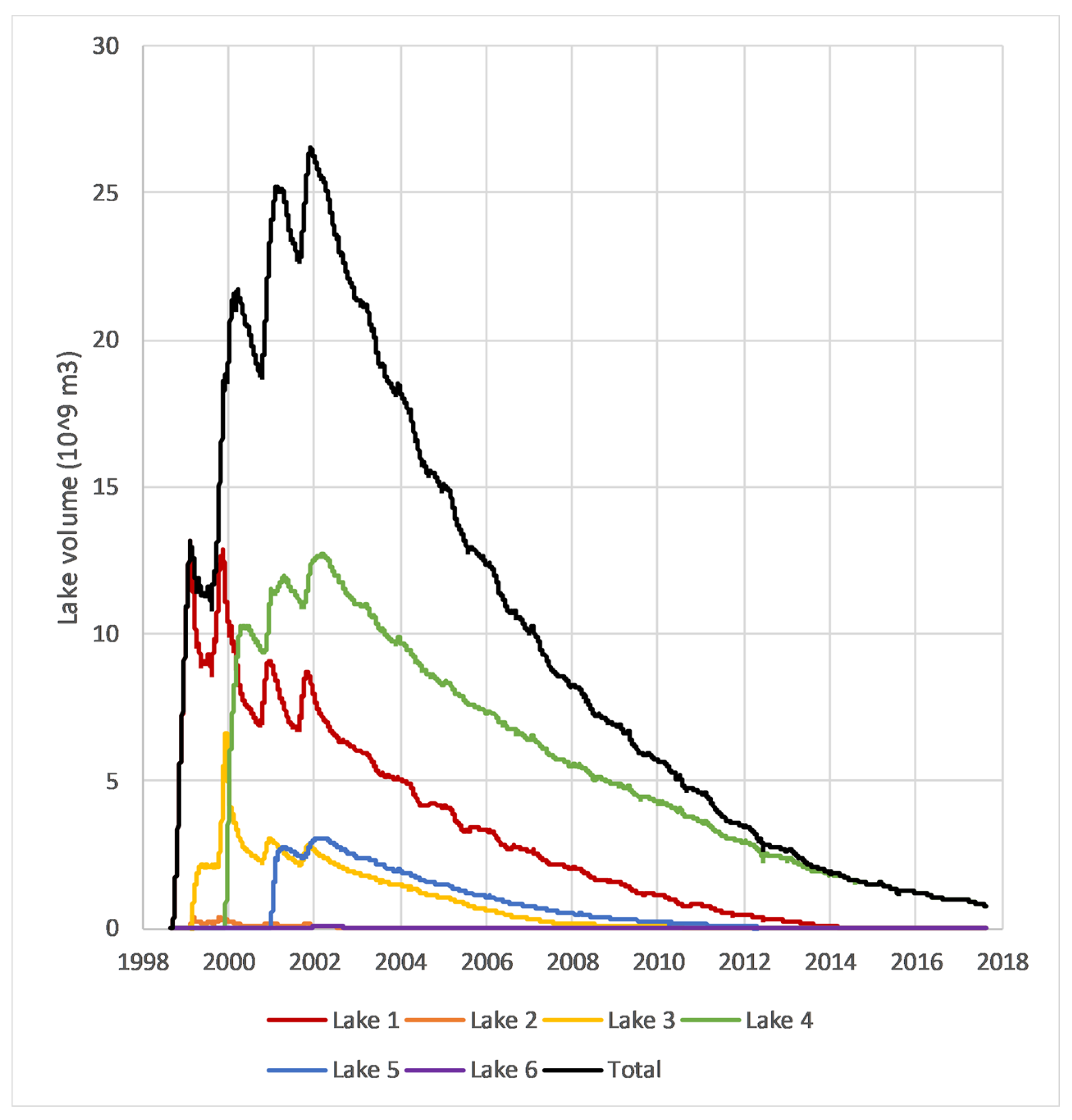
:Lakes in arid regions play an important role in regional water cycles and are a vital economic resource, but can fluctuate widely in area and volume. This study demonstrates the use of a multisensor satellite remote sensing method for the comprehensive monitoring of lake surface areas, water levels, and volume for the Toshka Lakes in southern Egypt, from lake formation in 1998 to mid-2017. Two spectral water indices were used to construct a daily time-series of surface area from the Advanced Very High Resolution Radiometer (AVHRR) and the Moderate Resolution Imaging Spectroradiometer (MODIS), validated by higher-resolution Landsat images. Water levels were obtained from analysis of digital elevation models from the Shuttle Radar Topography Mission (SRTM) and the Advanced Spaceborne Thermal Emission and Reflection Radiometer (ASTER), validated with ICESat Geoscience Laser Altimeter System (GLAS) laser altimetry. Total lake volume peaked at 26.54 × 10⁹ m3 in December 2001, and declined to 0.76 × 10⁹ m3 by August 2017. Evaporation accounted for approximately 86% of the loss, and groundwater recharge accounted for 14%. Without additional inflows, the last remaining lake will likely disappear between 2020 and 2022. The Enhanced Lake Index, a water index equivalent to the Enhanced Vegetation Index, was found to have lower noise levels than the Normalized Difference Lake Index. The results show that multi-platform satellite remote sensing provides an efficient method for monitoring the hydrology of lakes.
1. Introduction
1.1. Background: Remote Sensing of Lake Hydrology
The world’s ~117 million lakes and reservoirs [1] have an important role in the water and carbon cycles at regional scales, and provide a wide range of ecosystem services and economic benefits [2,3,4]. In some regions, lakes are known to be declining or disappearing due to disparate causes, ranging from climate change to human water withdrawals for agriculture, industry, and domestic consumption [5,6]. Lakes in arid regions are particularly sensitive to changes in local to regional hydrology [6,7,8], which is a troubling fact, given their disproportionate importance in the ecology and economic systems of these water-limited areas. Other anthropogenic impacts on lakes may also have severe consequences, such as the introduction of invasive species [9,10], overfishing [10,11], and pollution [12,13].
Remote sensing is widely used in limnology and lake management for identifying, measuring, and characterizing the properties of lakes [1,14,15,16]. Lake surface area has been successfully mapped using optical and microwave sensors in environments from the tropics to the poles [1,14,17,18,19,20,21,22,23], often using spectral indices such as the normalized difference water index (NDWI; [20,21]), the normalized difference lake index (NDLI; [18,23]), or the automated water extraction index (AWEI; [22]). Much early work on mapping the distribution and extent of lakes used optical sensors carried on the Landsat and SPOT (“Système probatoire d’observation de la Terre”, also rendered as “Satellite pour l’observation de la Terre”) series of satellites. Historically, issues of sensor calibration and radiometric quality, atmospheric correction, and data distribution hindered the development of fully automated, high-temporal resolution systems for lake monitoring using these optical remote sensing platforms. Since 2000, the launch of operational, global monitoring systems, such as the Moderate Resolution Imaging Spectroradiometer (MODIS) and the Sentinel satellite constellation, including products and/or tools for deriving surface reflectance from the raw top-of-atmosphere spectral radiance measurements, has enabled the development of automated algorithms for frequent monitoring of lake surface areas from space.
The vertical dimension of lake volume (water level or bathymetry) can be measured using laser altimetry [7,24,25,26,27,28] or radar altimetry [28,29,30,31,32]. Although it was only operational from 2003–2009, and experienced technical problems that limited its data collection to a few operational periods per year, the Geoscience Laser Altimeter System (GLAS) on the Ice, Cloud, and Land Elevation Satellite-1 (ICESat-1; [24]) provided spot measurements of water level for many lakes worldwide, and comparison of measurements between operational periods enabled the estimation of changes in water level. The use of satellite laser altimetry from space is likely to become far more widespread with the recent successful launch of ICESat-2.
Due in part to the influence of the oceanographic community, the science of water-level measurement from radar altimetry has matured rapidly, and been supported by a temporally overlapping series of platforms, including ERS-1 and -2, the Ocean Topography Experiment (TOPEX/Poseidon), Envisat, Jason-1 and -2 Ocean Surface Topography Mission (OSTM), and Cryosat-2. For the lake research and management community, the Global Reservoir and Lake Monitor (G-REALM; [33]) is a widely-used automated system for assimilating radar altimetry across multiple platforms for the development of long-term records of water-level change in large lakes worldwide. Compared to laser altimetry, satellite radar altimetry typically provides a coarser spatial resolution, making it suitable for only the largest lakes worldwide, but with the advantage of a long and continuous historical record and independence from the constraints of cloud cover.
Recently, a number of studies have used simultaneous analysis of lake area (via image classification) and water level (via altimetry) to derive changes in lake volume. In [34], the changing area and water level of Lake Victoria were measured using MODIS and ERS/Envisat, respectively, for a 22-year period. A similar approach was used for Lake Urmia in Iran [35], using MODIS with Envisat/Cryosat-2. The upcoming Surface Water and Ocean Topography (SWOT) satellite mission, scheduled for launch in 2021, will provide lake area and water level measurements from its Ka and Ku band radars, providing further support for remote sensing of changes in lake volume [36,37]. This objective has also been accomplished by combining remotely sensed images of lake area with water level estimates from a pre-existing digital elevation model (DEM) [38,39].
Other remote sensing methods for monitoring dynamics of water storage in lakes, wetlands, and other aquatic systems include the use of interferometric radar (InSAR) or satellite gravimetry. InSAR can be used to estimate water levels by analysis of double-bounce returns from the stems of inundated vegetation [40,41], due to the high interferometric coherence from these features, in contrast to the low coherence from open water. Alternatively, changes in water storage can be inferred from InSAR measurements of the displacement (uplift or subsidence) of the terrain surrounding large lakes [42]. Satellite gravimetry, using systems such as the Gravity Recovery and Climate Experiment (GRACE) or Gravity field and steady-state Ocean Circulation Explorer (GOCE), has been widely used to infer regional- to continental-scale changes in hydrology, due to the impact of changes in the mass of water in groundwater [43,44] and surfacewater systems [45,46] on the regional gravitational field. Recently, GRACE gravity data have been successfully shown to be capable of providing estimates of hydrologic change in finer-scale systems, such as individual lakes, via a modeling approach to downscale the regional GRACE signal, with results that match those from radar altimetry [47].
The study area for this work (the Toshka or Tushka Lakes in southern Egypt) has been the setting for several prior investigations using satellite remote sensing to monitor changes in lake hydrology. The methods and results of those prior studies will be discussed in Section 1.2 below. Following that, in Section 1.3, the dual objectives of this work are presented: First, to demonstrate and evaluate a set of methodological improvements that enable the construction of a fully-automated system for monitoring changes in surface area, water level, and volume in lakes; and second, to use this system to document the history of the Toshka Lakes at a higher temporal resolution and more rigorously and completely than previous studies.
1.2. Study Region
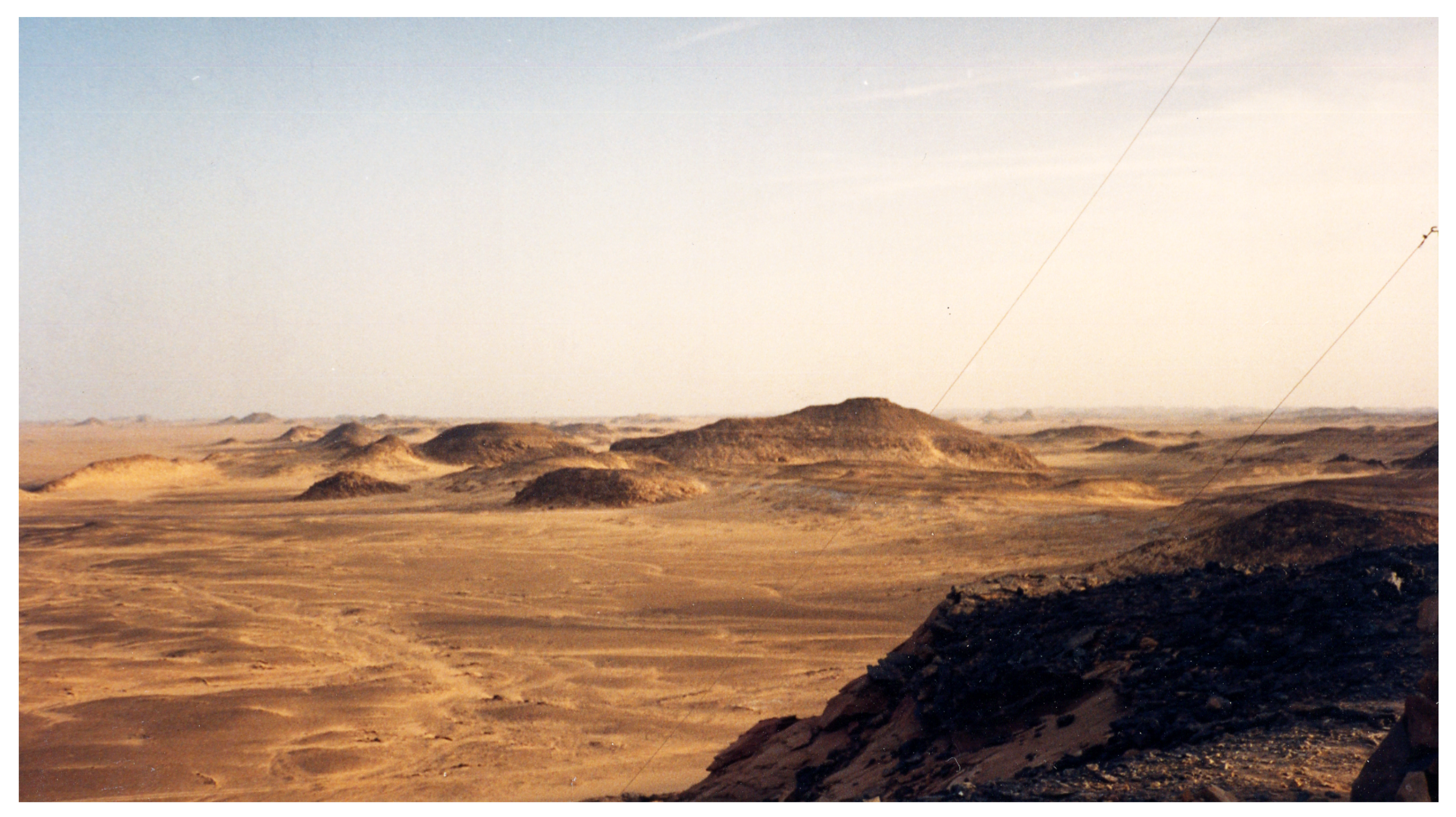
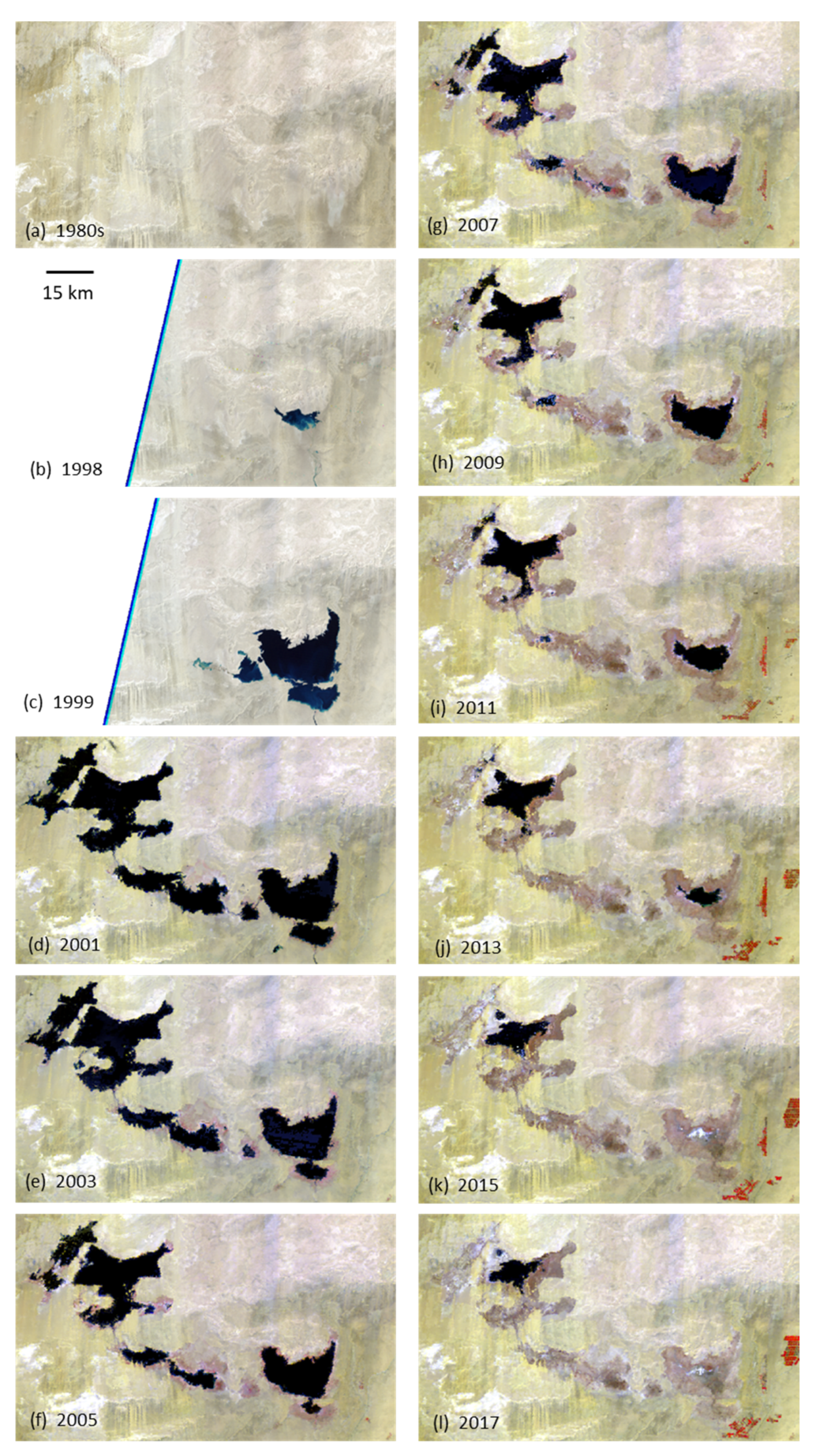
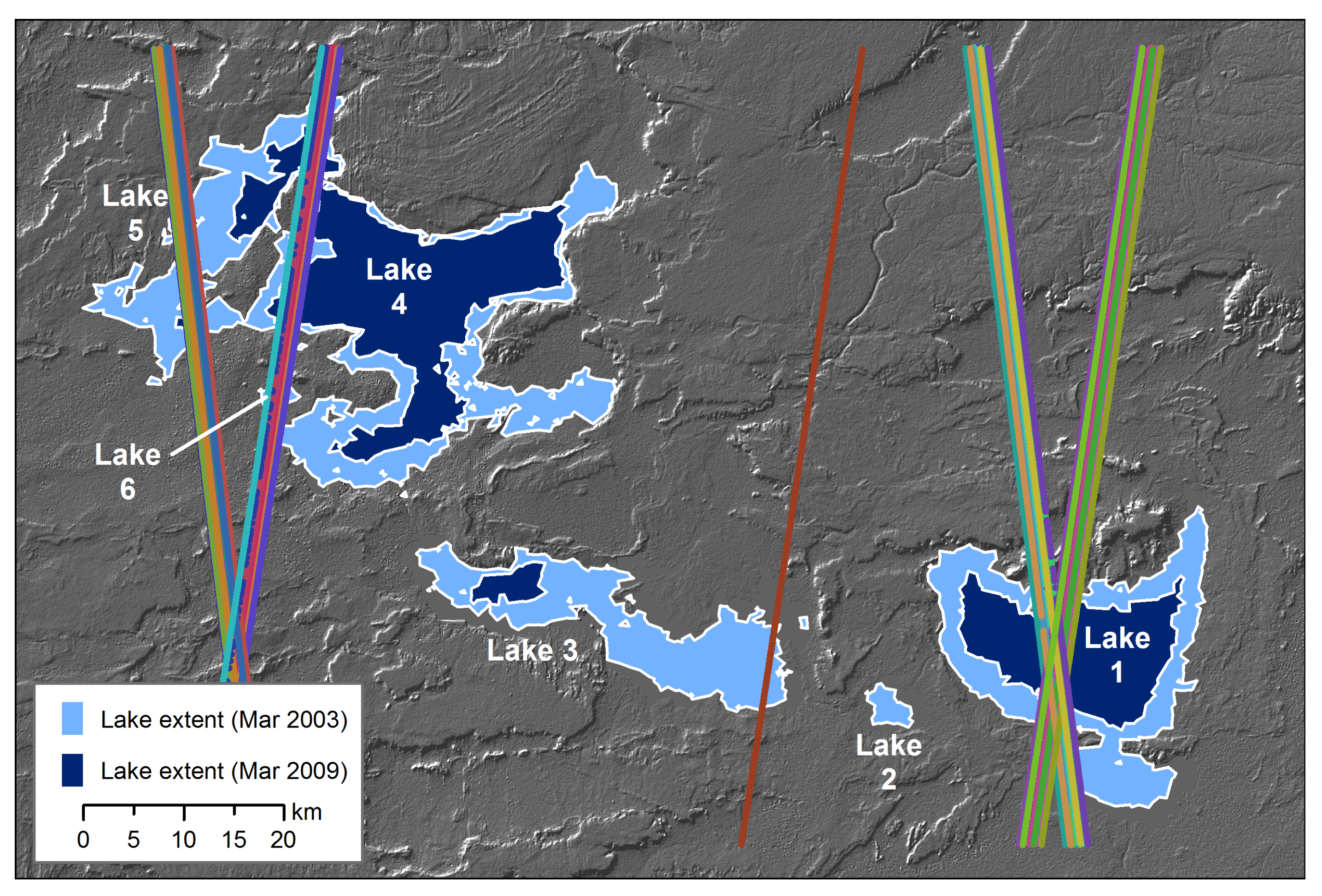
The Toshka Lakes basin is located in the Western Desert of southern Egypt, west of the Nile’s Lake Nasser reservoir (Figure 1a). Although there is evidence for river channels and lakes in the region during the middle Pleistocene [48], the region is currently a hyper-arid desert (Figure 2) and was devoid of surface water prior to the development of an artificial spillway and channel (22 km length) from Lake Nasser in 1978 to protect the dam during times of high flow on the Nile [49]. Beginning in September 1998, increasing water levels in the Nile brought Lake Nasser to the elevation of the spillway, leading to the formation of the first Toshka lake (Lake 1). As waters continued to rise during the late-1998/1999 flood season, and subsequent flood seasons up to 2001/2002, a series of additional lakes were formed by waters spilling out of Lake 1 into downstream basins to the west (Figure 1b). After 2002, water levels in the Toshka Lakes began dropping, and by mid-2017, only Lake 4 remained extant (Figure 3). During the early 2000s, a short-lived fishery developed on the lakes, with over 7000 tonnes produced in 2004 [50], but its growth was quickly halted and reversed by the salinization and eventual disappearance of the lakes. The formation and subsequent desiccation of the lakes also had a significant impact on local climate [51].
Due to the isolation of the region and the broad spatial scale of the lake basins, satellite remote sensing has been a primary source of information on the dynamic hydrology of the Toshka Lakes. The specific approaches have been varied, and are summarized in Table 1. What sets the present study apart from these earlier works is its combination of high-temporal frequency observation of lake surface area, water level, and volume, for the entire life cycle of the lakes, with comparisons among different methodological choices and data sources.
The first of these four prior studies, one by Chipman and Lillesand [7], used relatively coarse-resolution optical imagery from the Advanced Very High-Resolution Radiometer (AVHRR) and MODIS, in an adaptive, sub-pixel analysis algorithm to estimate the surface area of each lake on 145 dates, from lake formation in 1998 to mid-2006. The MODIS imagery used in this study was Level-1B (geometrically corrected top-of-atmosphere spectral radiance). Surface area measurements were validated by comparison to higher-resolution Landsat images. Water levels for four of the six lakes were measured using ICESat-1 GLAS, although Lake 3 had only a single date of GLAS measurements and thus could not be used to estimate rates of change in water level. For Lake 5, a pre-inundation digital elevation model (DEM) was obtained from the Shuttle Radar Topography Mission (SRTM) and was used to infer changes in water level as its basin filled and then began drying. Lake surface area reached a maximum of 1740 km2 in or around December 2001. The volume of Lake 5 (from the Shuttle Radar Topography Mission [SRTM] DEM) reached a maximum of 3.13 × 10⁹ m3 in February 2002. During the declining period, water levels in Lake 5 dropped by 7.41 [95% CI 7.00 to 7.82] mm/day (SRTM DEM) or 7.13 [6.77 to 7.49] mm/day (ICESat-1 GLAS). This 2007 study can be seen as a pilot project for the current study, which greatly expands and improves upon its data sources and methodologies.
Bastawesy et al. [52] used Advanced Spaceborne Thermal Emission and Reflection Radiometer (ASTER) imagery from 2002 and SPOT-4 imagery from 2006 to measure the extent of the lakes in those two years. Lake areas were derived from a manual thresholding process in the near-infrared band of each sensor, resulting in a binary land/water image. A DEM was also digitized from pre-inundation topographic maps, and used to estimate water level and volume in each lake on the dates of the ASTER and SPOT-4 images. The 2002 total surface area was reported as 1591 km2, and was 937 km2 in 2006. Volume (of all lakes) was 25.26 × 10⁹ m3 in 2002 and 12.67 × 10⁹ m3 in 2006. The rate of decline in water level during the four-year interval was reported as (approximately) 7 mm/day. Bastawesy et al. also predicted that, in the absence of additional inflows, the larger lakes would disappear in 2012 (Lake 3), 2014 (Lake 1), and 2020 (Lake 4).
Abdelsalam et al. [53] used a one-class parallelepiped image classification approach to map lake extent on approximately 14 dates from 1998–2007. They reported a maximum area of ~1586 km2 in August 2001, the closest of their image dates to the actual maximum. The projected date for the disappearance of the lakes was given as March 2011. The difference between this and the 2020 projection from [52] was due to the fact that [52] projected each lake’s evolution individually, while [53] projected only the aggregated total area of all lakes, using a linear model.
Finally, Hereher [23] analyzed 14 MODIS images, one per year from 2000–2013 during the month of March, to estimate lake surface area. Atmospherically corrected (surface reflectance) versions of the MODIS red, near-infrared, and shortwave-infrared bands were extracted from the MOD13Q1 vegetation index product, and used in two spectral indices: the land surface water index (LSWI; [54]) and the NDLI ([18]). A threshold in each index was used to separate land and water, in a binary fashion as in [52]. The largest surface area reported (in March of 2002) was 1664 km2, three to four months after the actual maximum area was reached in December 2001. In addition to reporting the surface area of the lakes, [23] also examined the extent of irrigated agricultural development between the Toshka Lakes and Lake Nasser, a large undertaking supported by water withdrawn from the Nile.
1.3. Objectives
This study had two overarching objectives. The first was to develop and test methodological improvements in the use of remote sensing for monitoring water storage in lakes. This contributes to the development of an automated system that integrates a wide range of remotely sensed data sources and analytical methods to simultaneously measure trends in lake surface area, water level, and volume, building upon and improving the methods previously described in [7]. The second objective was to apply these data and methods for a comprehensive assessment of the evolution of the Toshka Lakes over the two decades of their existence, producing daily estimates of each lake’s surface area, water level, and volume. To meet these dual objectives, the following tasks were performed:
Lake surface area assessment:
- Quantitative comparison of two remotely sensed spectral lake indices, NDLI and the enhanced lake index (ELI), for lake surface area estimation, using an adaptive algorithm for sub-pixel analysis.
- Construction of a daily time-series of lake surface area over two decades (1998–2017) from AVHRR and MODIS imagery.
- Validation of the AVHRR/MODIS lake surface area dataset in comparison to higher-resolution image sources.
Water-level assessment:
- Quantitative comparison of multiple algorithms and data sources for estimating water levels from integration of DEMs and lake surface area datasets.
- Construction of a daily time-series of water levels and depth statistics for each lake.
- Validation of the water level dataset by comparison to laser altimetry.
Lake volume assessment:
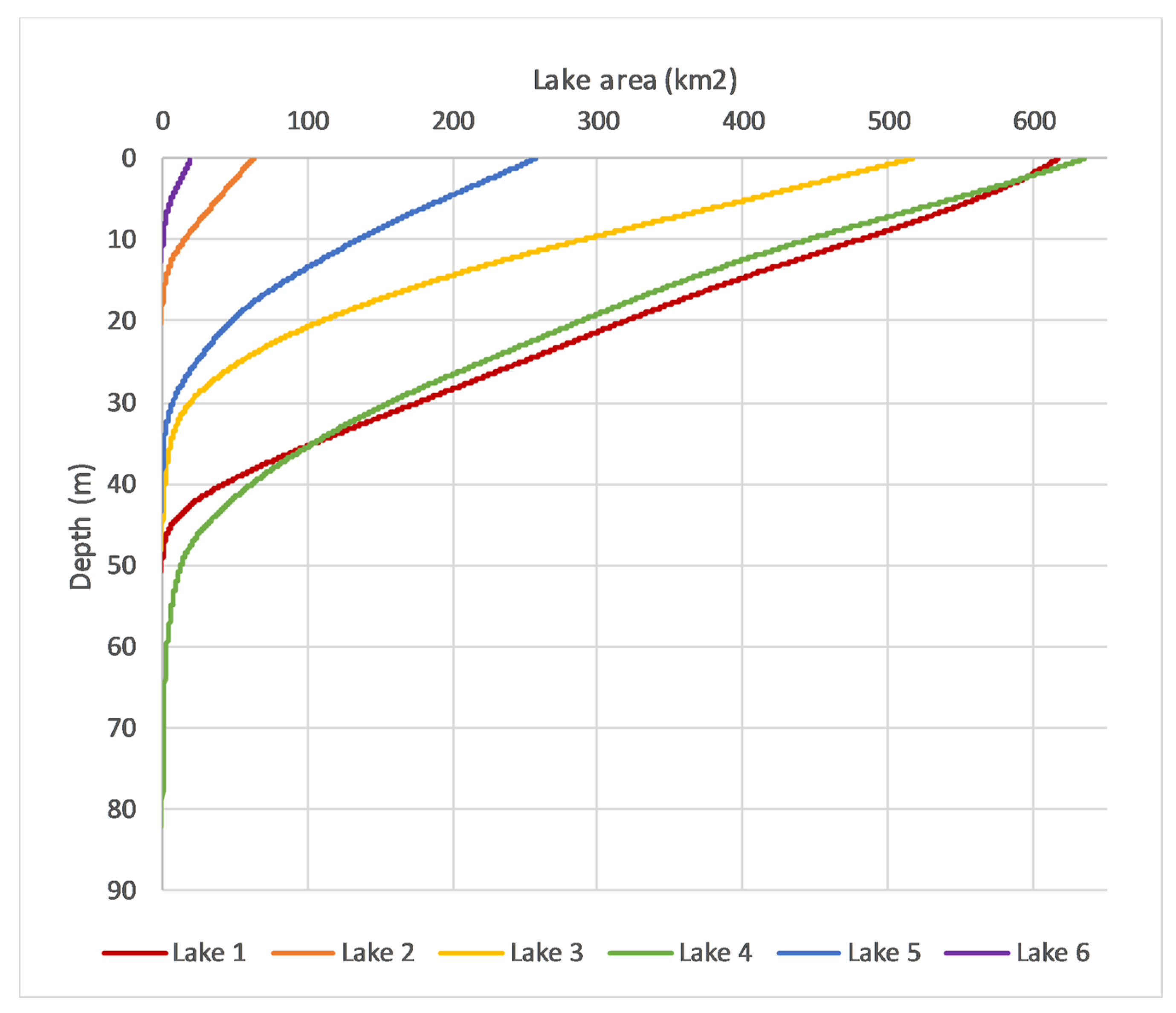
- Construction of hypsographic curves for each lake, representing the relationship between lake surface area and water level.
- Derivation of a daily time-series of lake volume, by cross-referencing the lake surface area dataset and each lake’s hypsographic curve.
Note that, while the term “validation” is used here for the lake surface area and water level assessments, no direct, in-situ measurements of area or water level were available. Instead, in both cases the validation process involved comparison to another remotely sensed data source. For surface area, the measurements made here from coarse-resolution sensors (AVHRR and MODIS) were compared to equivalent measurements from much higher-resolution Landsat images. For water level, the results from different algorithms and DEMs were compared to ICESat-1 GLAS laser altimetry, a completely independent and previously-validated source of water level data [7,25,27].
In the course of addressing the first objective, the following hypotheses were tested (stated here informally, rather than in formal null-and-alternative hypothesis language):
Hypothesis 1: The use of sub-pixel analytical methods allows for coarser-resolution imagery (e.g., AVHRR and MODIS) to produce lake surface area estimates that are compatible with each other and equivalent to those from much higher-resolution imagery (Landsat).
Hypothesis 2: A new numerical lake index for multispectral optical imagery (ELI) will yield better (i.e., less noisy) estimates of lake surface area than the existing index, NDLI.
Hypothesis 3: DEMs obtained when lakes are at low water-levels, or dry, can be combined with maps of surface area to provide estimates of water level that are similar to those from laser altimetry.
Rather than being framed in terms of specific hypotheses to test, the second objective involves production of new datasets, providing a comprehensive, daily record of the dynamic expansion and contraction of the Toshka lakes during the two decades from 1998–2017, encompassing the formation of all six lakes, and the subsequent disappearance of five of the six. Comparison to measured evaporation rates (from nearby Lake Nasser) supports inferences about the relative proportion of water lost to evaporation vs. groundwater recharge. Finally, the results of this study will provide guidance for similar remote-sensing-based assessments of lake hydrology in other regions.
This study goes beyond the prior work on the Toshka lakes in a variety of ways. Unlike [23] and [53], it includes analysis of lake water level and volume, and provides a much higher temporal resolution analysis of surface area (812 dates of imagery, vs. 14 and 27, respectively in those prior studies). While [7] and [52] included water level and volume, this new study again provides a much higher temporal resolution and more than a decade of additional data. Additionally, in contrast to [7], it provides water levels and volumes for all lakes, and in contrast to [52], it provides a comparison between water level estimates derived from DEM analysis and from satellite laser altimetry. It also defines and evaluates a new lake index (ELI), compares two different remotely-sensed sources of DEMs, and compares two different algorithms for obtaining water levels from DEMs.
2. Materials and Methods
2.1. Data Sources
The data used in this study are listed in Table 2, with references. For lake surface area, the primary source was the complete time series of Terra and Aqua MODIS 16-day composites (2000–2017), with AVHRR images from 1998–2000, and higher resolution Landsat-5, -7, and -8 images and SPOT-5 images used for validation (Landsat) and threshold selection (SPOT). Water level, mean depth, and lake volume were derived from DEMs from SRTM in 2000 and from stereoscopic ASTER band 3 (NIR) imagery from 2014–2017. ICESat-1 GLAS laser altimetry data (2003–2009) were used for validation of water levels.
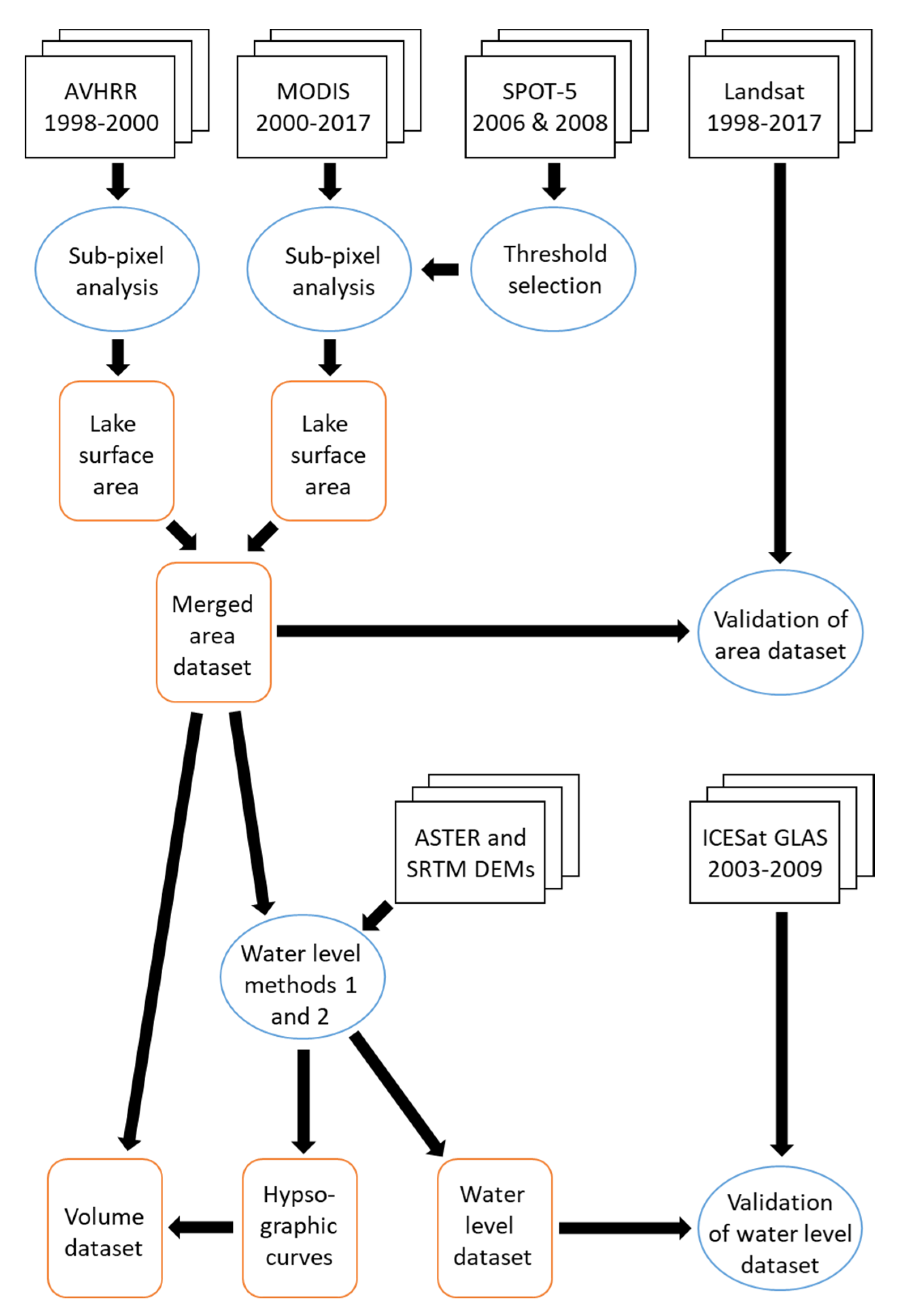
The methods used to analyze these data and derive time-series of lake surface area, water level, and volume are summarized in Figure 4, and are discussed in detail in the following subsections.
2.2. Lake Surface Area
The process used to estimate lake surface area was based upon that described in [7]. For this study, the MODIS MOD13Q1/MYD13Q1 16-day composite product (hereafter “MOD13”) was used, rather than the Level-1B imagery of [7]. MOD13 includes two vegetation indices, the normalized difference vegetation index (NDVI) and the enhanced vegetation index (EVI; [61]), as well as surface reflectance in selected MODIS bands, data quality flags, and other data. Two lake indices were derived from MOD13, the aforementioned NDLI [18,23] and the new ELI.
NDLI is given by Equation (1):
where RRED and RNIR are the spectral reflectance or spectral radiance in red and near-infrared wavelength bands, respectively. Note that NDLI is equivalent to a sign-reversed version of NDVI; i.e., values of NDLI >0 are increasingly likely to be water, and are equivalent to NDVI <0. Due to the high correlation between visible wavelength spectral bands, NDLI is generally very similar to the NDWI [20,21] but does not require the use of a green-wavelength band.
Similarly, the new index ELI (Equation 2) is a sign-reversed version of EVI:
where RNIR, RRED, and RBLUE are the near-infrared, red, and blue wavelength bands, C1 and C2 are wavelength-specific aerosol resistance terms (6 and 7.5, respectively, for MODIS, [61]), and G is a gain factor of −2.5 (versus +2.5 for EVI). High values of ELI (= low values of EVI) are increasingly likely to represent water.
For this study, NDLI and ELI were each used to map lake surface area, using the same methodology. Firstly, the data were reprojected to the Universal Transverse Mercator (UTM) zone 36 North coordinate system and subset to the study region. Secondly, a constant threshold value (0 for NDLI, −0.04 for ELI) was used to create a binary land/water mask for each date. Thirdly, the binary-mask time series was smoothed by comparing each pixel on date t to its value on dates t-8 and t+8 days (i.e., the previous and subsequent MOD13 dataset; prior to the first Aqua image in mid-2002, with only Terra imagery available, this was t-16 and t+16). If the pixel’s land/water value differed on both the comparison dates, it was switched. Finally, the fractional extent of water for mixed pixels along shorelines (i.e., the boundaries between land and water) was estimated using a linear mixture model [7].
This produced two time series (nFrac and eFrac, derived from NDLI and ELI, respectively) of maps showing the fractional (0.0 to 1.0) extent of water within each pixel. Summing up the fractions for each pixel of a lake and multiplying by the pixel area (based on the sensor’s spatial resolution) yielded the surface area for each lake on each date.
For the period prior to the first Terra MODIS image (February 2000), the coarser-resolution AVHRR sensor was used in a similar process. Due to the lack of a blue-wavelength band on AVHRR, only an NDLI-based AVHRR dataset could be constructed, and it was used with both the NDLI and ELI versions of the MODIS time series. The same process was used to derive much finer-scale maps of lake area from a series of Landsat images. These data (30 m resolution, or nearly two orders of magnitude finer in resolution than MODIS) were used to validate the coarser-resolution lake area measurements. Likewise, the same process was used with two dates of even higher resolution (10 m) SPOT-5 multispectral images (2006-11-07 and 2008-04-20) to determine the appropriate threshold (-0.04) for the MODIS ELI land/water mask, by comparing MODIS land/water masks with a variety of different thresholds to area measurements from the two SPOT-5 images.
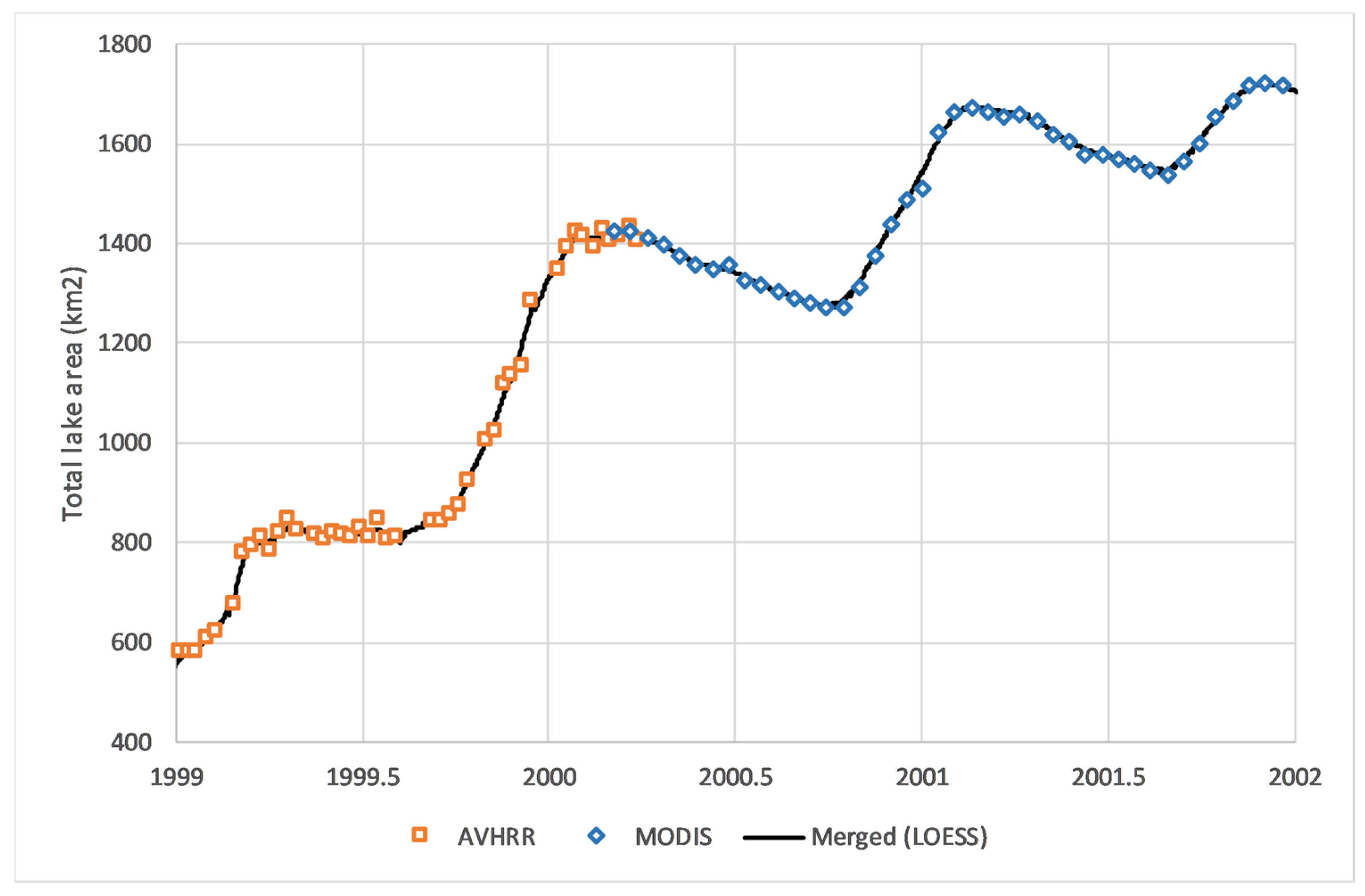
The AVHRR (1998–2000) and MODIS (2000–2017) lake surface area time-series were merged using a nonparametric locally estimated scatterplot smoothing (LOESS) model, interpolating area to a daily timestep using the minimal value of α = 5 data points (nominally 40 days in the post-2002 era when both Terra and Aqua were available) to minimize smoothing. Figure 5 shows this LOESS model for the period of the transition from AVHRR to MODIS (1999-01-01 to 1992-01-01). While the AVHRR data are coarser-resolution and noisier, the alignment between it and MODIS is very close.
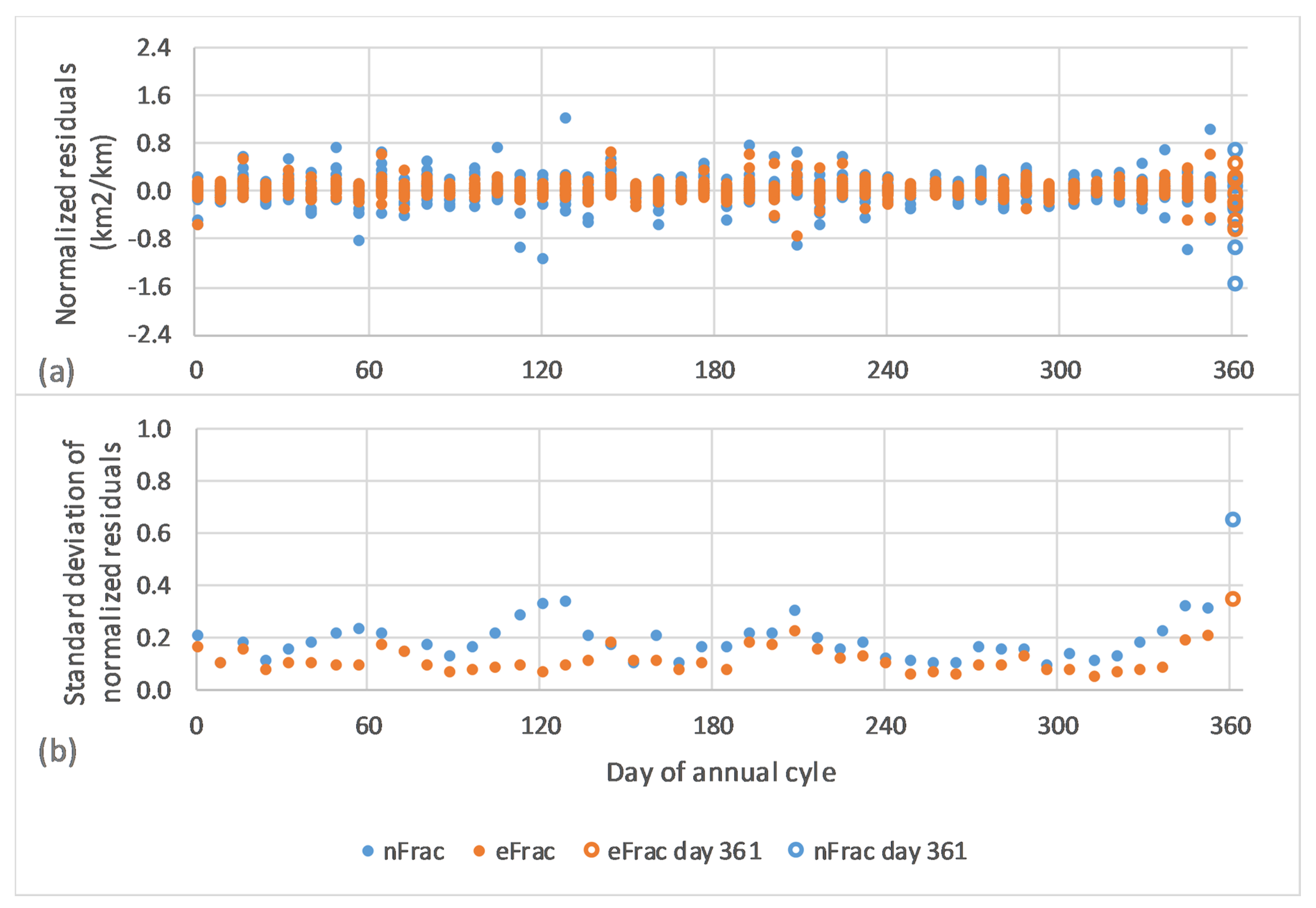
The NDLI- and ELI-derived lake area time series (nFrac and eFrac) were compared based on their detrended residuals, i.e., the individual observations minus the LOESS model, which are here considered to represent noise. Because the magnitude of this noise increases as the lake circumference (and zone of mixed pixels along the shoreline) increases, the residuals were normalized by dividing them by the square root of lake area, giving units of km2/km. These normalized residuals were used to evaluate the relative performance of NDLI and ELI as sources in the lake area algorithm. The results are presented in more detail in Section 3, but are shown and discussed briefly here because the choice between NDLI and ELI affected the subsequent methods.
Examination of the residuals showed three extreme outliers among the 750 MODIS image dates: Julian days 161 and 169 in 2012, and day 353 of 2007. Visual examination of these images confirmed that these should be excluded from the analysis due to artifacts in the MOD13 source data. In addition, the lake area values from both NDLI and ELI for Aqua MODIS day 361 were anomalously noisy, yielding larger residuals in many years than other dates (Figure 6), potentially as a result of the 16-day compositing process. (The NASA Land Processes Distributed Active Archive Center (LP DAAC) reported a known issue with the MODIS MYD13Q1 v6.0 16-day composite product, resulting in “unexpected missing data in the last cycles of each year”. The issue is being addressed in the reprocessed v6.1.) All the day 361 images were thus removed as well, and the nFrac and eFrac time series were recalculated.
As shown in Figure 6, the eFrac time series (derived from ELI rather than NDLI) had generally smaller residuals relative to its LOESS model. Thus, eFrac was used as the definitive lake surface area dataset for all subsequent analyses.
The final step in the lake surface area process involved validation of area measurements by comparison to higher-resolution Landsat images. Two Landsat path/row combinations were needed to cover the area (paths 175 and 176, row 44) with Lakes 1 and 2 in path 175 and the remaining lakes in path 176. For each Landsat image, the areas of each lake were compared to the corresponding daily LOESS-interpolated AVHRR/MODIS eFrac lake area measurement. Because each Landsat pixel covers an area only 1/69th as large as a 250 m resolution MODIS pixel, the Landsat images provided a more precise estimate of lake area.
2.3. Water Level, Mean Depth, and Volume
Water level was derived by cross-referencing the lake surface area dataset (Section 2.2 above) with a digital elevation model (DEM). Based on the water level, mean and maximum depths were calculated on each date, hypsographic curves were computed for each lake, and lake volumes were estimated. Two different methods were used for the water level analysis, and the results were validated using ICESat-1 GLAS laser altimetry data, which were completely independent of the DEM-based methods.
The first DEM for the study region was obtained from the SRTM [62] dataset. This DEM was produced using interferometric analysis of synthetic aperture radar (SAR) data from 11–22 February 2000. The basins for Lakes 1-4 had already filled by this date, so the bathymetry of those lakes could not be determined from SRTM.
A second DEM was developed from photogrammetric analysis of stereoscopic ASTER bands 3N and 3B. Twelve individual ASTER DEMs were used, from images in 2014–2017 when all lakes except Lake 4 had dried up, thus allowing the bathymetry of each lake basin (except Lake 4) to be mapped directly. The ASTER DEMs had large vertical offsets relative to SRTM (and to each other), and various other artifacts. The cause of these offsets is undetermined, but they are reflective of the fact that the relative accuracy of these DEMs (i.e., the reported difference in elevation between any two points within a single DEM, compared to their true difference in elevation) is better than their absolute accuracy (the absolute elevations of points in the DEM compared to their true elevations); the latter are expected to be better than 25 m root mean squared error (RMSE) [59]. To prepare these DEMs for use, the following process was followed:
- Calculate each ASTER tile’s mean and standard deviation of elevation differences from the SRTM DEM, using a subset of the area with no visible artifacts.
- Adjust the ASTER DEMs to match the SRTM DEM by adding each tile’s mean elevation difference, excluding areas that are more than three standard deviations from the SRTM elevation and were not covered by water at the time of the SRTM mission.
- In the ASTER tile covering the (small) remaining water in the Lake 4 basin, exclude ASTER DEM pixels falling within the extent of the water area.
- Create an initial mosaic of all ASTER DEM tiles, averaging elevation values in areas of overlap.
- Aggregate to 150 m spatial resolution, and convert grid cells to points.
- Delete points in no-data areas (areas where the ASTER DEM was more than three standard deviations from SRTM, or within the remaining Lake 4 water area).
- Perform a “tension” spline interpolation (weight = 0.1, 100 points per region for local approximation) to fill in the gaps.
The result was an ASTER DEM mosaic for the entire area, with artifacts removed and the small residual area covered by water in Lake 4 modeled by spline interpolation. This ASTER DEM was used to calculate elevation, depth, and volume for all lakes on all dates, while the SRTM DEM was used as a comparison on Lake 5 only. Table 3 lists the ASTER DEM tiles used in the DEM mosaic.
Two different methods were used to estimate water levels from the lake surface area maps and the DEMs. In Method 1, the shoreline (where pixel fractional water extent crossed 0.5) was identified from the eFrac surface area maps, and the mean elevation of this line was found in the DEM(s). In Method 2, the area of pixels at or below each increment of elevation was calculated directly from the ASTER DEM, and then the observed area on a given date (from eFrac) was used to look up the corresponding water level that would produce that observed area.
For each lake, the water levels derived from these two methods were compared to the ICESat-1 GLAS laser altimeter measurements of water level on the corresponding dates, averaging all 70 m-diameter GLAS footprints that fell on each lake surface on each orbit (Figure 7). A total of 2390 laser spots on 54 separate orbit tracks were used. Some orbit tracks crossed more than one lake, resulting in 76 combinations of lake and orbit track. An additional 644 laser spots on 16 orbit tracks were not used due to abnormally high noise levels in the GLAS data; these noisy tracks (also discussed in [7]) had standard deviations of the GLAS measurements for individual lakes from 0.1 to 0.7 m, and were identified and removed based on that basis.
Hypsographic curves [63,64] for each lake were constructed, for use in estimating lake volumes on each date. These curves relate lake area (on the X axis) to depth (Y axis). Using the lake area vs. water level data from Method 2, points representing the measured values of these two variables on each date were plotted, and then a LOESS model was used to interpolate values for water level at 0.1 km2 increments of lake area, from 0.1 km2 to the maximum areal extent of each lake. This hypsographic curve was then used as a look-up table, to determine the mean depth and total volume for each lake on each date, based on its surface area, in increments of 0.1 km2.
3. Results
3.1. Lake Surface Area
Both the nFrac and eFrac processes yielded time series of lake surface area from MODIS, from February 2000 through August 2017. These were merged with coarser-resolution AVHRR data, and interpolated to a daily timestep. As discussed in Section 2.2, comparison of the residuals suggested that eFrac had a lower noise level than nFrac—after removal of all MODIS day 361 images and three other outliers, the standard deviation of the normalized residuals was 0.20 km2/km for nFrac and 0.12 km2/km for eFrac. Thus, the eFrac version was used as the definitive lake area dataset.
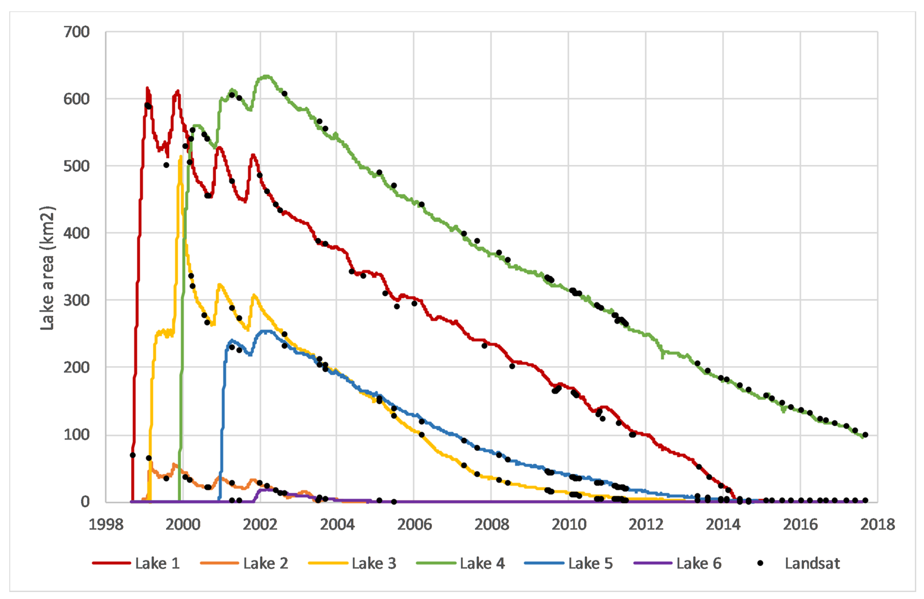
Figure 8 shows the time series of lake surface area for all six individual lakes, along with 206 validation points (black dots) obtained from comparison of the MODIS and AVHRR data to higher-resolution Landsat images (194 during the MODIS era and 12 during the AVHRR era). The lake system as a whole reached a maximum area on or around 1 December 2001, at 1722 km2. Individual lakes reached their maxima on different dates (Table 4).
Using the 206 Landsat-derived lake surface area measurements as “truth”, the mean absolute error (MAE) in the AVHRR/MODIS eFrac time series was 18.7% of lake area, but this was dominated by dates on which lake areas were very small—excluding those with lake areas below 5 km2 (n = 42), the MAE for remaining dates (n = 164) was 4.8% of the lake area. A scatterplot of lake area estimates from Landsat vs from AVHRR/MODIS is shown in Figure 9.
3.2. Water Level, Mean Depth, and Volume
As described in Section 2.3, two methods were used to estimate water level by combining lake surface area maps with the ASTER DEM mosaic. Method 1 involved measuring the average elevation of the observed shoreline of the lake, while Method 2 involved constructing a histogram of elevations within each lake basin from the DEM (i.e., the count of pixels at each increment of elevation) and finding the elevation at which the cumulative histogram matched the observed lake area in km2.
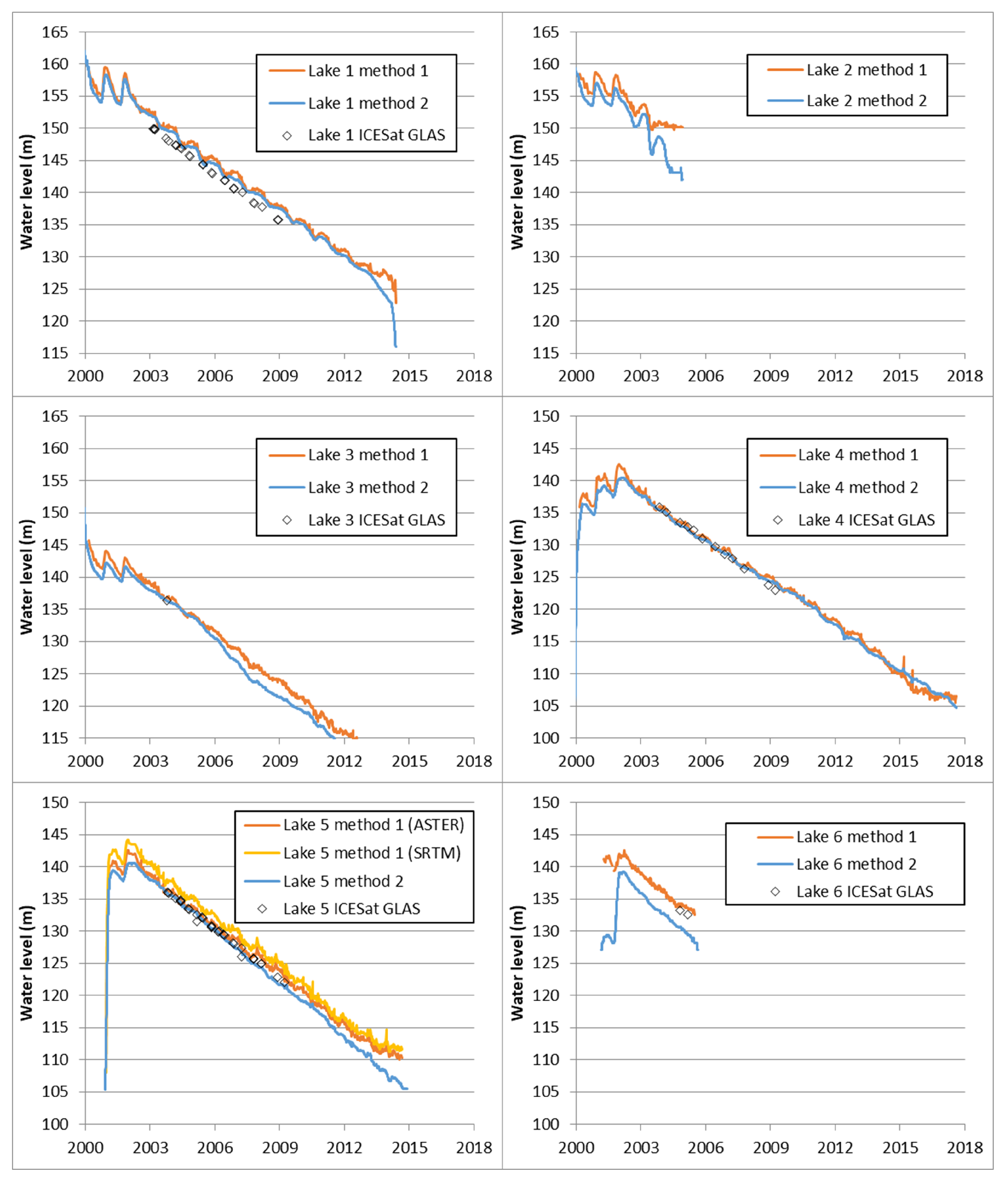
Figure 10 shows a comparison of the results of these two methods for all six lakes (for Lake 5, whose basin was not filled until after the date of the SRTM DEM; Method 1 was also used with the SRTM data as an additional comparison). ICESat-1 GLAS laser altimetry points are also shown for each lake crossed by one of the ICESat orbit tracks (see map in Figure 7). Because each GLAS orbit track across a given lake may include many individual laser measurements, each lake’s GLAS water level estimate can be described in terms of both a mean and standard deviation. The mean values (for 76 combinations of lake and orbit track) are used in Figure 11 and Table 5; the standard deviations ranged from 0.016 to 0.091 m, with a mean standard deviation of 0.041 m.
In general, water levels increase and decrease prior to 2003, due to seasonal inflows from the Nile, and then decrease continuously and approximately linearly from 2003 onward, indicating a consistent net water loss due to evaporation and groundwater recharge. Table 6 shows the date on which each lake reached its maximum average depth. In principle, the date of maximum average depth could differ from the date of maximum surface area, but in this case, the dates are the same for all lakes except Lake 5 are the same (cf. Table 4).
The rates of change in water level during the 2003–2009 operational period of the ICESat-1 GLAS mission are given in Table 5; these results are less reliable for Lakes 2 and 6 due to their small size and short duration of existence during this time period.
Hypsographic curves for all six lakes are shown in Figure 12. The lowermost range of the curve for Lake 4 is uncertain, because it is based on the basin’s bathymetric ASTER DEM with spline interpolation to estimate elevations within its late-2017 water extent (Section 2.3 above). In each case, zero on the depth axis is set based on the maximum areal extent of the lake during the entire 1998–2017 (AVHRR and MODIS) time series.
4. Discussion
Both the dual objectives of this study were achieved: (1) Various methodological improvements in the remote sensing of water storage in lakes were described and implemented in an automated system for measurement of lake surface area, water level, and volume; and (2) this system was used to develop new, comprehensive, highly detailed datasets on the life cycle of the Toshka lakes since their formation 20 years ago.
All three of the informally-stated hypotheses from Section 1.3 were borne out. For Hypothesis 1, the adaptive sub-pixel analysis algorithm for estimation of lake surface area worked well across a wide range of spatial scales; the output from the 1000 m resolution AVHRR imagery merged smoothly with the 250 m MODIS output (Figure 5), and both were generally consistent with the 30 m Landsat (Figure 8 and Figure 9) and 10 m SPOT imagery. As noted in [22], the widely used process of setting a “hard” land/water threshold in a near-infrared band or spectral index can cause problems due to slight variations in scene illumination, sensor calibration, or imperfectly corrected atmospheric conditions. The use of an adaptive algorithm for this threshold is conceptually preferable, as is the modeling of sub-pixel water fraction for shoreline pixels, rather than the use of a simple binary classification.
For Hypothesis 2, the version of the lake area algorithm using ELI had a lower noise level than the version with NDLI (Figure 6). However, like its equivalent vegetation index EVI, ELI does require the presence of a blue spectral band, in addition to the red and near-infrared bands used in NDLI.
For Hypothesis 3, the two methods for estimating water levels by combining lake area maps and DEMs gave generally similar results. The reported trends in water level (Table 5) were virtually identical for Lakes 1 and 4; for Lakes 3 and 5, Method 2 gave rates of decline that were 14% and 10% faster than Method 1. The observed rates of decline in ICESat-1 GLAS were 3% and 11% faster than the DEM-based methods for Lakes 1 and 4 respectively; for Lake 5, ICESat’s rate fell between those from the two DEM-based methods. The recent launch of ICESat-2 should provide an excellent source for lake water measurements at a finer scale than those obtainable by satellite radar altimetry.
The data produced in this study can be used to address other questions about the past and future of the Toshka lakes, such as the partitioning of water losses between evaporation and recharge, and the anticipated expiration of the last remaining lake. With no outlet for surface water discharge from this closed depression, the decline in water levels is attributable to two factors: evaporation and groundwater recharge. Elsawwaf et al. [65] used data from floating rafts on Lake Nasser, just east of the Toshka Lakes, to estimate evaporation rates from the reservoir. The mean daily evaporation rates at the two stations closest to the Toshka Lakes spillway were 5.78 mm/day (Allaqi) and 5.90 mm/day (Abusembel). Comparing these rates and the mean of Methods 1 and 2 for water level measurement in this study suggests that approximately 86% of the water loss observed here was via evaporation, with 14% via groundwater recharge. The groundwater recharge fraction was highest for Lake 3 and lowest for Lake 4.
As noted in Section 1.2, Bastawesy et al. [52] reported a rate of decline in water level during from 2002–2006 of (approximately) 7 mm/day. During the same time period, this study finds similar rates (the average for the four largest lakes is 6.9 mm/day with Method 1, and 7.0 mm/day with Method 2). Bastawesy et al. also predicted that, in the absence of additional inflows, the larger lakes would disappear in 2012 (Lake 3), 2014 (Lake 1), and 2020 (Lake 4). Those predictions were accurate for Lakes 3 and 1. In this study, Lake 4 is projected to disappear between 2020 and 2022, barring any further inputs of surface water from Lake Nasser.
While this study has applied its methods to one particular set of lakes with their own history and circumstances, the methods should be broadly applicable to many other lakes and reservoirs that have experienced declining water levels due to evaporation. Globally, the problem of water loss from artificial reservoirs is of increasing concern [66,67] and the use of automated, remote-sensing-based methods to characterize these losses and to assess variability in these systems is very promising [33], though the latter focuses on water levels in only the largest lakes worldwide.
5. Conclusions
Both of the overarching objectives of this study were successfully addressed. An automated system (objective 1) was demonstrated for monitoring changes in the surface area, water level, and volume of lakes, using data from multiple earth-observation satellites. Surface area measurements were produced using an adaptive algorithm that estimates fractional (sub-pixel) estimates of water extent along lake shorelines, using a newly proposed Enhanced Lake Index (ELI), parallel to the Enhanced Vegetation Index (EVI). The results are consistent across two orders of magnitude in spatial scale. Water-level measurements and trends can be derived from satellite laser altimetry or from analysis of digital elevation models (DEMs) using two different methods. Changes in volume can be inferred from surface area trends and hypsographic curves, which in turn can be derived from DEMs during periods of low water. While presenting several methodological improvements, e.g., the use of ELI for mapping water extent and comparison of two algorithms and two DEM data sources for water level estimation, this study also shows how these methods could be implemented in an end-to-end automated system for lake monitoring.
Applied to the Toshka Lakes in southern Egypt (objective 2), these methods have provided the most comprehensive daily record of the formation, expansion, and decline of lakes over the past two decades, and have enabled the inference of the amount of groundwater recharge from each lake basin. With the development of new sources of wide-scale, high-temporal frequency imagery from constellations such as Sentinel and Planet Labs, and the recent launch of a new laser altimeter on ICESat-2, the next decade should see a rapid expansion in remotely sensed assessments of lake hydrology.
Author Contributions
conceptualization, J.W.C.; methodology, J.W.C.; software, J.W.C.; validation, J.W.C.; formal analysis, J.W.C.; investigation, J.W.C.; resources, J.W.C.; data curation, J.W.C.; writing—original draft preparation, J.W.C.; writing—review and editing, J.W.C.; visualization, J.W.C.; project administration, J.W.C.; funding acquisition, J.W.C.
Funding
Portions of this work were funded by the NASA Terrestrial Hydrology Program through grant #NNG06GE46G. The APC was funded by Dartmouth College’s Open-Access Publication Equity Fund.
Acknowledgments
MODIS and ASTER data were provided courtesy of NASA Land Processes DAAC, AVHRR data courtesy of NOAA, Landsat data courtesy of USGS EROS Center, ICESat-1 GLAS data courtesy of the National Snow and Ice Data Center, and SRTM data courtesy of the Jet Propulsion Laboratory and USGS EROS Center.
Conflicts of Interest
The author declares no conflict of interest.
References
- Verpoorter, C.; Kutser, T.; Seekell, D.A.; Tranvik, L.J. A global inventory of lakes based on high-resolution satellite imagery. Geophys. Res. Lett. 2014, 41, 6396–6402. [Google Scholar] [CrossRef] [Green Version]
- Winter, T.C.; Woo, M.K. Hydrology of lakes and wetlands. In Surface Water Hydrology; Wolman, M.G., Riggs, H.C., Eds.; Geological Society of America: Boulder, CO, USA, 1990; pp. 159–188. ISBN 9780813754666. [Google Scholar]
- Postel, S.; Carpenter, S. Freshwater ecosystem services. In Nature’s Services: Societal Dependence on Natural Ecosystems; Daily, G.C., Ed.; Island Press: Washington, DC, USA, 1997; pp. 195–214. ISBN 1-55963-475-8. [Google Scholar]
- Tranvik, L.J.; Downing, J.A.; Cotner, J.B.; Loiselle, S.A.; Striegl, R.G.; Ballatore, T.J.; Dillon, P.; Finlay, K.; Fortino, K.; Knoll, L.B.; et al. Lakes and reservoirs as regulators of carbon cycling and climate. Limnol. Oceanogr. 2009, 54, 2298–2314. [Google Scholar] [CrossRef] [Green Version]
- Smith, L.C.; Sheng, Y.; MacDonald, G.M.; Hinzman, L.D. Disappearing arctic lakes. Science 2005, 308, 1429. [Google Scholar] [CrossRef] [PubMed]
- Wurtsbaugh, W.A.; Miller, C.; Null, S.E.; DeRose, R.J.; Wilcock, P.; Hahnenberger, M.; Howe, F.; Moore, J. Decline of the world’s saline lakes. Nat. Geosci. 2017, 10, 816–821. [Google Scholar] [CrossRef]
- Chipman, J.W.; Lillesand, T.M. Satellite-based assessment of the dynamics of new lakes in southern Egypt. Int. J. Remote Sens. 2007, 28, 4365–4379. [Google Scholar] [CrossRef]
- Micklin, P. The past, present, and future Aral Sea. Lakes Reserv. Res. Manag. 2010, 15, 193–213. [Google Scholar] [CrossRef]
- Walsh, J.R.; Carpenter, S.R.; Vander Zanden, M.J. Invasive species triggers a massive loss of ecosystem services through a trophic cascade. Proc. Natl. Acad. Sci. USA 2016, 113, 4081–4085. [Google Scholar] [CrossRef] [PubMed]
- Ogutu-Ohwayo, R. The decline of the native fishes of lakes Victoria and Kyoga (East Africa) and the impact of introduced species, especially the Nile perch, Lates niloticus, and the Nile tilapia, Oreochromis niloticus. Environ. Biol. Fish. 1990, 27, 81–96. [Google Scholar] [CrossRef]
- Allan, J.D.; Abell, R.; Hogan, Z.E.B.; Revenga, C.; Taylor, B.W.; Welcomme, R.L.; Winemiller, K. Overfishing of inland waters. BioScience 2005, 55, 1041–1051. [Google Scholar] [CrossRef]
- Rashed, M.N. Monitoring of environmental heavy metals in fish from Nasser Lake. Environ. Int. 2001, 27, 27–33. [Google Scholar] [CrossRef]
- Driedger, A.G.; Dürr, H.H.; Mitchell, K.; Van Cappellen, P. Plastic debris in the Laurentian Great Lakes: A review. J. Great Lakes Res. 2015, 41, 9–19. [Google Scholar] [CrossRef] [Green Version]
- Chipman, J.W.; Olmanson, L.G.; Gitelson, A.A. Remote Sensing Methods for Lake Management: A Guide for Resource Managers and Decision-Makers; North American Lake Management Society: Madison, WI, USA, 2009. [Google Scholar]
- Alsdorf, D.E.; Rodríguez, E.; Lettenmaier, D.P. Measuring surface water from space. Rev. Geophys. 2007, 45, 2006RG000197. [Google Scholar] [CrossRef]
- Gao, H.; Birkett, C.; Lettenmaier, D.P. Global monitoring of large reservoir storage from satellite remote sensing. Water Resour. Res. 2012, 48, W09504. [Google Scholar] [CrossRef]
- Melack, J.M.; Hess, L.L.; Sippel, S. Remote sensing of lakes and floodplains in the Amazon Basin. Remote Sens. Rev. 1994, 10, 127–142. [Google Scholar] [CrossRef]
- Morriss, B.; Hawley, R.; Chipman, J.; Andrews, L.; Catania, G.; Hoffman, M.; Lüthi, P.; Neumann, T. A ten-year record of supraglacial lake evolution and rapid drainage in West Greenland using an automated processing algorithm for multispectral imagery. Cryosphere 2013, 7, 1869–1877. [Google Scholar] [CrossRef]
- Yang, X.; Chen, L. Evaluation of automated urban surface water extraction from Sentinel-2A imagery using different water indices. J. Appl. Remote Sens. 2017, 11, 026016. [Google Scholar] [CrossRef]
- Gao, B.C. NDWI—A normalized difference water index for remote sensing of vegetation liquid water from space. Remote Sens. Environ. 1996, 58, 257–266. [Google Scholar] [CrossRef]
- McFeeters, S.K. The use of the Normalized Difference Water Index (NDWI) in the delineation of open water features. Int. J. Remote Sens. 1996, 17, 1425–1432. [Google Scholar] [CrossRef]
- Feyisa, G.L.; Meilby, H.; Fensholt, R.; Proud, S. Automated Water Extraction Index: A new technique for surface water mapping using Landsat imagery. Remote Sens. Environ. 2014, 140, 23–35. [Google Scholar] [CrossRef]
- Hereher, M.E. Environmental monitoring and change assessment of Toshka lakes in southern Egypt using remote sensing. Environ. Earth Sci. 2015, 73, 3623–3632. [Google Scholar] [CrossRef]
- Wang, X.; Cheng, X.; Gong, P.; Huang, H.; Li, Z.; Li, X. Earth science applications of ICESat/GLAS: A review. Int. J. Remote Sens. 2011, 32, 8837–8864. [Google Scholar] [CrossRef]
- Zhang, G.; Xie, H.; Kang, S.; Yi, D.; Ackley, S.F. Monitoring lake level changes on the Tibetan Plateau using ICESat altimetry data (2003–2009). Remote Sens. Environ. 2011, 115, 1733–1742. [Google Scholar] [CrossRef]
- Arsen, A.; Crétaux, J.F.; Berge-Nguyen, M.; del Rio, R.A. Remote sensing-derived bathymetry of Lake Poopó. Remote Sens. 2013, 6, 407–420. [Google Scholar] [CrossRef]
- Ye, Z.; Liu, H.; Chen, Y.; Shu, S.; Wu, Q.; Wang, S. Analysis of water level variation of lakes and reservoirs in Xinjiang, China using ICESat laser altimetry data (2003–2009). PLoS ONE 2017, 12, e0183800. [Google Scholar] [CrossRef]
- Swenson, S.; Wahr, J. Monitoring the water balance of Lake Victoria, East Africa, from space. J. Hydrol. 2009, 370, 163–176. [Google Scholar] [CrossRef]
- Birkett, C.M. Synergistic remote sensing of Lake Chad: Variability of basin inundation. Remote Sens. Environ. 2000, 72, 218–236. [Google Scholar] [CrossRef]
- Crétaux, J.F.; Birkett, C. Lake studies from satellite radar altimetry. C. R. Geosci. 2006, 338, 1098–1112. [Google Scholar] [CrossRef]
- Berry, P.A.M.; Garlick, J.D.; Freeman, J.A.; Mathers, E.L. Global inland water monitoring from multi-mission altimetry. Geophys. Res. Lett. 2005, 32, L16401. [Google Scholar] [CrossRef]
- Nielsen, K.; Stenseng, L.; Andersen, O.B.; Villadsen, H.; Knudsen, P. Validation of CryoSat-2 SAR mode based lake levels. Remote Sens. Environ. 2015, 171, 162–170. [Google Scholar] [CrossRef] [Green Version]
- Birkett, C.M.; Ricko, M.; Beckley, B.D.; Yang, X.; Tetrault, R.L. G-REALM: A lake/reservoir monitoring tool for drought monitoring and water resources management. Abstract #H23P-02. In Proceedings of the American Geophysical Union Fall Meeting, American Geophysical Union, Washington, DC, USA, 2017. [Google Scholar]
- Tong, X.; Pan, H.; Xie, H.; Xu, X.; Li, F.; Chen, L.; Luo, X.; Liu, S.; Chen, P.; Jin, Y. Estimating water volume variations in Lake Victoria over the past 22 years using multi-mission altimetry and remotely sensed images. Remote Sens. Environ. 2016, 187, 400–413. [Google Scholar] [CrossRef]
- Tourian, M.J.; Elmi, O.; Chen, Q.; Devaraju, B.; Roohi, S.; Sneeuw, N. A spaceborne multisensor approach to monitor the desiccation of Lake Urmia in Iran. Remote Sens. Environ. 2015, 156, 349–360. [Google Scholar] [CrossRef]
- Solander, K.C.; Reager, J.T.; Famiglietti, J.S. How well will the Surface Water and Ocean Topography (SWOT) mission observe global reservoirs? Water Resour. Res. 2016, 52, 2123–2140. [Google Scholar] [CrossRef] [Green Version]
- Biancamaria, S.; Lettenmaier, D.P.; Pavelsky, T.M. The SWOT mission and its capabilities for land hydrology. In Remote Sensing and Water Resources; Cazenave, A., Champollion, N., Benveniste, J., Chen, J., Eds.; Springer Nature: Basel, Switzerland, 2016; pp. 117–147. ISBN 978-3-319-32448-7. [Google Scholar]
- Delaney, K.B.; Evans, S.G. The 2000 Yigong landslide (Tibetan Plateau), rockslide-dammed lake and outburst flood: Review, remote sensing analysis, and process modelling. Geomorphology 2015, 246, 377–393. [Google Scholar] [CrossRef]
- Yang, R.; Zhu, L.; Wang, J.; Ju, J.; Ma, Q.; Turner, F.; Guo, Y. Spatiotemporal variations in volume of closed lakes on the Tibetan Plateau and their climatic responses from 1976 to 2013. Clim. Chang. 2017, 140, 621–633. [Google Scholar] [CrossRef]
- Alsdorf, D.E.; Melack, J.M.; Dunne, T.; Mertes, L.A.; Hess, L.L.; Smith, L.C. Interferometric radar measurements of water level changes on the Amazon flood plain. Nature 2000, 404, 174. [Google Scholar] [CrossRef] [PubMed]
- Jaramillo, F.; Brown, I.; Castellazzi, P.; Espinosa, L.; Guittard, A.; Hong, S.H.; Rivera-Monroy, V.H.; Wdowinski, S. Assessment of hydrologic connectivity in an ungauged wetland with InSAR observations. Environ. Res. Lett. 2018, 13, 024003. [Google Scholar] [CrossRef] [Green Version]
- Zhao, W.; Amelung, F.; Doin, M.P.; Dixon, T.H.; Wdowinski, S.; Lin, G. InSAR observations of lake loading at Yangzhuoyong Lake, Tibet: Constraints on crustal elasticity. Earth Planet. Sci. Lett. 2016, 449, 240–245. [Google Scholar] [CrossRef]
- Lo, M.H.; Famiglietti, J.S.; Reager, J.T.; Rodell, M.; Swenson, S.; Wu, W.Y. GRACE-Based Estimates of Global Groundwater Depletion. In Terrestrial Water Cycle and Climate Change: Natural and Human-Induced Impacts; Tang, Q., Oki, T., Eds.; American Geophysical Union: Washington, DC, USA, 2016; pp. 137–146. ISBN 978-1-118-97176-5. [Google Scholar]
- Frappart, F.; Ramillien, G. Monitoring groundwater storage changes using the Gravity Recovery and Climate Experiment (GRACE) satellite mission: A review. Remote Sens. 2018, 10, 829. [Google Scholar] [CrossRef]
- Eom, J.; Seo, K.W.; Ryu, D. Estimation of Amazon River discharge based on EOF analysis of GRACE gravity data. Remote Sens. Environ. 2017, 191, 55–66. [Google Scholar] [CrossRef]
- Gouweleeuw, B.T.; Kvas, A.; Gruber, C.; Gain, A.K.; Mayer-Gürr, T.; Flechtner, F.; Güntner, A. Daily GRACE gravity field solutions track major flood events in the Ganges–Brahmaputra Delta. Hydrol. Earth Syst. Sci. 2018, 22, 2867. [Google Scholar] [CrossRef]
- Ni, S.; Chen, J.; Wilson, C.R.; Hu, X. Long-term water storage changes of Lake Volta from grace and satellite altimetry and connections with regional climate. Remote Sens. 2017, 9, 842. [Google Scholar] [CrossRef]
- Maxwell, T.A.; Issawi, B.; Haynes, C.V. Evidence for Pleistocene lakes in the Tushka region, south Egypt. Geology 2010, 38, 1135–1138. [Google Scholar] [CrossRef] [Green Version]
- Abdel-Motaleb, M.; Saad, M.B.A. Calibration of an Ogee weir. In Proceedings of the 29th International Association for Hydraulic Engineering and Research, Beijing, China, 16–21 September 2001; pp. 796–803. [Google Scholar]
- El-Shabrawy, G.M.; Dumont, H.J. The Toshka Lakes. In The Nile: Origin, Environments, Limnology, and Human Use; Dumont, H.J., Ed.; Springer: Dordrecht, The Netherlands, 2009; pp. 157–162. ISBN 978-1-4020-9725-6. [Google Scholar]
- Hereher, M.E. Effects of land use/cover change on regional land surface temperatures: Severe warming from drying Toshka lakes, the Western Desert of Egypt. Natl. Hazards 2017, 88, 1789–1803. [Google Scholar] [CrossRef]
- Bastawesy, M.A.; Khalaf, F.I.; Arafat, S.M. The use of remote sensing and GIS for the estimation of water loss from Tushka lakes, southwestern desert, Egypt. J. Afr. Earth Sci. 2008, 52, 73–80. [Google Scholar] [CrossRef]
- Abdelsalam, M.G.; Youssef, A.M.; Arafat, S.M.; Alfarhan, M. Rise and demise of the New Lakes of Sahara. Geosphere 2008, 4, 375–386. [Google Scholar] [CrossRef]
- Xiao, X.; Boles, S.; Liu, J.; Zhuang, D.; Frolking, S.; Li, C.; Salas, W.; Moore III, B. Mapping paddy rice agriculture in southern China using multi-temporal MODIS images. Remote Sens. Environ. 2005, 95, 480–492. [Google Scholar] [CrossRef]
- Didan, K. NASA LP DAAC. MOD13Q1: MODIS/Terra Vegetation Indices 16-Day L3 Global 250 m SIN Grid V006; NASA EOSDIS Land Processes DAAC, USGS Earth Resources Observation and Science (EROS) Center: Sioux Falls, SD, USA, 2015.
- Didan, K. NASA LP DAAC. MYD13Q1: MODIS/Aqua Vegetation Indices 16-Day L3 Global 250 m SIN Grid V006; NASA EOSDIS Land Processes DAAC, USGS Earth Resources Observation and Science (EROS) Center: Sioux Falls, SD, USA, 2015.
- USGS EROS Center. Landsat Data Archive; USGS Earth Resources Observation and Science (EROS) Center: Sioux Falls, SD, USA, 2017.
- Kobrick, M.; Crippen, R. NASA Shuttle Radar Topography Mission Global 1 Arc Second V003; NASA EOSDIS Land Processes DAAC, USGS Earth Resources Observation and Science (EROS) Center: Sioux Falls, SD, USA, 2013.
- US/Japan ASTER Science Team. AST14DEM: ASTER Digital Elevation Model V003; NASA EOSDIS Land Processes DAAC, USGS Earth Resources Observation and Science (EROS) Center: Sioux Falls, SD, USA, 2001. [CrossRef]
- Zwally, H.J.; Schutz, R.; Bentley, C.; Bufton, J.; Herring, T.; Minster, J.; Spinhirne, J.; Thomas, R. GLA14: GLAS/ICESat L2 Global Land Surface Altimetry Data, Release 33; NASA National Snow and Ice Data Center Distributed Active Archive Center: Boulder, CO, USA, 2011. [Google Scholar]
- Huete, A.; Didan, K.; Miura, T.; Rodriguez, E.P.; Gao, X.; Ferreira, L.G. Overview of the radiometric and biophysical performance of the MODIS vegetation indices. Remote Sens. Environ. 2002, 83, 195–213. [Google Scholar] [CrossRef]
- Van Zyl, J.J. The Shuttle Radar Topography Mission (SRTM): A breakthrough in remote sensing of topography. Acta Astron. 2001, 48, 559–565. [Google Scholar] [CrossRef]
- Håkanson, L. On lake form, lake volume and lake hypsographic survey. Geografiska Annaler Ser. A Phys. Geogr. 1977, 59, 1–29. [Google Scholar] [CrossRef]
- Zolá, R.P.; Bengtsson, L. Three methods for determining the area–depth relationship of Lake Poopó, a large shallow lake in Bolivia. Lakes Reserv. Res. Manag. 2007, 12, 275–284. [Google Scholar] [CrossRef]
- Elsawwaf, M.; Willems, P.; Pagano, A.; Berlamont, J. Evaporation estimates from Nasser Lake, Egypt, based on three floating station data and Bowen ratio energy budget. Theor. Appl. Climatol. 2010, 100, 439–465. [Google Scholar] [CrossRef]
- Jaramillo, F.; Destouni, G. Local flow regulation and irrigation raise global human water consumption and footprint. Science 2015, 350, 1248–1251. [Google Scholar] [CrossRef] [PubMed]
- Mekonnen, M.M.; Hoekstra, A.Y. The blue water footprint of electricity from hydropower. Hydrol. Earth Syst. Sci. 2012, 16, 179–187. [Google Scholar] [CrossRef] [Green Version]
Figure 1.
Maps of the study area. (a) Location of the Toshka Lakes region in southern Egypt; (b) lakes 1 through 6 superimposed on shaded relief (lake extents from February 2002).
Figure 1.
Maps of the study area. (a) Location of the Toshka Lakes region in southern Egypt; (b) lakes 1 through 6 superimposed on shaded relief (lake extents from February 2002).

Figure 2.
The Western Desert near Lake Nasser and the Toshka region (photo by the author).

Figure 3.
Formation, expansion, and desiccation of the Toshka Lakes. (a) Landsat image mosaic from the 1980s, prior to lake formation; (b–c) Landsat images of the eastern half of the Toshka Lakes region, 1998–1999; (d–l) Terra/Aqua Moderate Resolution Imaging Spectroradiometer (MODIS) images from odd-numbered years 2001–2017.

Figure 4.
Schematic diagram of the data and methods used in this study.

Figure 5.
Combination of lake surface area measurements from the Advanced Very High Resolution Radiometer (AVHRR; orange squares) and MODIS (blue diamonds) with interpolation using a locally estimated scatterplot smoothing (LOESS) regression model (black line) at a daily timestep. Area (in km2) is total for all six lakes.

Figure 6.
Comparison of residuals from lake surface area time-series nFrac and eFrac, as a function of the seasonal cycle (Julian Day). (a) Normalized residuals (km2/km) for all years, by day; (b) standard deviation of normalized residuals (km2/km) by day. Excluded data from Aqua MODIS Day 361 are shown as open circles.

Figure 7.
Ice, Cloud, and Land Elevation Satellite-1 (ICESat-1) Geoscience Laser Altimeter System (GLAS) laser altimeter orbit tracks (colored lines), March 2003–March 2009.
Figure 7.
Ice, Cloud, and Land Elevation Satellite-1 (ICESat-1) Geoscience Laser Altimeter System (GLAS) laser altimeter orbit tracks (colored lines), March 2003–March 2009.

Figure 8.
Lake surface area (km2) for each lake, 1998–2017. Colored lines are merged AVHRR/MODIS; black dots are individual lake measurements from Landsat, for validation.
Figure 8.
Lake surface area (km2) for each lake, 1998–2017. Colored lines are merged AVHRR/MODIS; black dots are individual lake measurements from Landsat, for validation.

Figure 9.
Scatterplot of lake surface area (km2) with coarse-resolution sensor area (MODIS or AVHRR) on the X axis and fine-resolution area (Landsat) on the Y axis.
Figure 9.
Scatterplot of lake surface area (km2) with coarse-resolution sensor area (MODIS or AVHRR) on the X axis and fine-resolution area (Landsat) on the Y axis.

Figure 10.
Comparison of methods for estimating water level (in colored lines) for all six lakes, with validation data from ICESat-1 GLAS laser altimetry (black diamonds).
Figure 10.
Comparison of methods for estimating water level (in colored lines) for all six lakes, with validation data from ICESat-1 GLAS laser altimetry (black diamonds).

Figure 11.
Lake volume (109 m3 = 1 km3), 1998–2017. Total of Lakes 1–6 shown in black.

Figure 12.
Hypsographic curves for each lake, relating lake area to depth (from AST14 DEMs).


Table 1.
Prior remote sensing studies of the hydrology of the Toshka Lakes.
| Time | Data Sources | Outcomes | Reference |
|---|---|---|---|
| 1998–2006 | 145 MODIS Level-1B/AVHRR images; Landsat; ICESat GLAS; SRTM DEM | Lake area (all lakes); water level and volume (Lake 5 only) | Chipman & Lillesand 2007 [7] |
| 2002 and 2006 | 7 ASTER/SPOT-4 images; DEM digitized from topographic maps | Lake area; water level & volume; evaporation | Bastawesy et al. 2008 [52] |
| 1998–2007 | 27 Landsat/ASTER images; SRTM DEM | Lake area; geologic/geomorphological controls | Abdelsalam et al. 2008 [53] |
| 2000–2013 | 14 MODIS MOD13 images | Lake area; vegetation/soils in riparian zone | Hereher 2015 [23] |
Table 2.
Remote sensing data sources.
| Data Source | Resolution | Dates | Role |
|---|---|---|---|
| Terra Moderate Resolution Imaging Spectroradiometer (MODIS) 16-day vegetation index composite V.006 (MOD13Q1) [55] | 250 m | 403 images: 2000-02-18 to 2017-08-13 | Lake surface area |
| Aqua MODIS 16-day vegetation index composite V.006 (MYD13Q1) [56] | 250 m | 349 images: 2002-07-04 to 2017-08-21 | Lake surface area |
| Advanced Very High Resolution Radiometer (AVHRR), Level-1B Local Area Coverage (LAC) | 1100 m | 62 images: 1998-09-26 to 2000-03-27 | Lake surface area |
| Landsat-5 Thematic Mapper (TM), Landsat-7 Enhanced Thematic Mapper (ETM+), and Landsat-8 Operational Land Imager (OLI) [57] | 30 m | 100 images: 1984-09-13 to 2017-09-15 | Lake surface area (validation) |
| SPOT-5 High Resolution Geometric (HRG) multispectral | 10 m | 2006-11-07 and 2008-04-20 | Threshold selection |
| Shuttle Radar Topography Mission (SRTM) digital elevation model (DEM) [58] | 30 m | 2000-02-11 to 2000-02-22 | Water level (Lake 5 only) |
| Advanced Spaceborne Thermal Emission and Reflection Radiometer (ASTER), DEMs from bands 3N and 3B (AST14DEM) [59] | 15 m | 12 DEMs: 2014-11-18 to 2017-10-09 | Water level and volume |
| Ice, Cloud, and Land Elevation Satellite (ICESat)-1 Geoscience Laser Altimeter System (GLAS) [60] | 70 m | 54 orbit tracks: 2003-02-28 to 2009-03-29 | Water level (validation) |
Table 3.
Advanced Spaceborne Thermal Emission and Reflection Radiometer (ASTER) DEM tiles (AST14) and their measured offsets from the SRTM DEM.
Table 3.
Advanced Spaceborne Thermal Emission and Reflection Radiometer (ASTER) DEM tiles (AST14) and their measured offsets from the SRTM DEM.
| Year | Day | Date | Region | Offset Mean (m) | Offset Stdev (m) |
|---|---|---|---|---|---|
| 2017 | 234 | 2017-08-22 | northeast | −24.22 | 10.94 |
| 2017 | 234 | 2017-08-22 | southeast | −23.72 | 11.17 |
| 2017 | 282 | 2017-10-09 | northwest | −5.77 | 6.00 |
| 2017 | 282 | 2017-10-09 | southwest | −4.35 | 6.23 |
| 2016 | 296 | 2016-10-22 | north-center | −22.38 | 6.12 |
| 2016 | 296 | 2016-10-22 | south-center | −18.87 | 8.16 |
| 2015 | 101 | 2015-04-11 | northwest | −23.66 | 9.27 |
| 2015 | 101 | 2015-04-11 | southwest | −21.68 | 11.98 |
| 2015 | 117 | 2015-04-27 | northwest | −11.68 | 12.70 |
| 2015 | 238 | 2015-08-26 | east | −13.23 | 7.49 |
| 2014 | 322 | 2014-11-18 | north-center | −10.86 | 9.44 |
| 2014 | 322 | 2014-11-18 | south-center | −17.95 | 11.00 |
Table 4.
Maximum surface area and date of maximum for each lake.
| Lake 1 | Lake 2 | Lake 3 | Lake 4 | Lake 5 | Lake 6 | Total | |
|---|---|---|---|---|---|---|---|
| Area (km2) | 617 | 63 | 515 | 634 | 255 | 19 | 1722 |
| Date of max. | 1999-02-05 | 1999-02-26 | 1999-12-13 | 2002-03-14 | 2002-04-06 | 2002-03-14 | 2001-12-01 |
Table 5.
Observed rates of change in water level (mm/day) from 2003–2009.
| Lake 1 | Lake 2 | Lake 3 | Lake 4 | Lake 5 | Lake 6 | |
|---|---|---|---|---|---|---|
| Method 1 (ASTER) | −6.57 | −4.04 | −7.01 | −5.96 | −6.86 | −6.78 |
| Method 1 (SRTM) | −7.04 | |||||
| Method 2 | −6.56 | −14.12 | −8.02 | −5.98 | −7.52 | −8.00 |
| Mean of M1 & M2 | −6.57 | −9.08 | −7.52 | −5.97 | −7.19 | −7.39 |
| ICESat GLAS | −6.74 | −6.60 | −7.10 |
Table 6.
Maximum average depth and date of maximum for each lake.
| Lake 1 | Lake 2 | Lake 3 | Lake 4 | Lake 5 | Lake 6 | Total | |
|---|---|---|---|---|---|---|---|
| Average depth (m) | 21.4 | 6.9 | 12.8 | 20.1 | 12.0 | 4.0 | 21.3 |
| Date of max | 1999-02-05 | 1999-02-26 | 1999-12-13 | 2002-03-14 | 2002-02-10 | 2002-03-14 | 1999-02-05 |
Table 7.
Maximum volumes and dates of maximum for each lake.
| Lake 1 | Lake 2 | Lake 3 | Lake 4 | Lake 5 | Lake 6 | Total | |
|---|---|---|---|---|---|---|---|
| Volume (109 m3) | 13.18 | 0.43 | 6.61 | 12.72 | 3.05 | 0.08 | 26.54 |
| Date of maximum | 1999-02-05 | 1999-02-26 | 1999-12-13 | 2002-03-14 | 2002-03-14 | 2002-03-14 | 2001-12-02 |
© 2019 by the author. Licensee MDPI, Basel, Switzerland. This article is an open access article distributed under the terms and conditions of the Creative Commons Attribution (CC BY) license (http://creativecommons.org/licenses/by/4.0/).
Share and Cite
MDPI and ACS Style
Chipman, J.W. A Multisensor Approach to Satellite Monitoring of Trends in Lake Area, Water Level, and Volume. Remote Sens. 2019, 11, 158. https://0-doi-org.brum.beds.ac.uk/10.3390/rs11020158
AMA Style
Chipman JW. A Multisensor Approach to Satellite Monitoring of Trends in Lake Area, Water Level, and Volume. Remote Sensing. 2019; 11(2):158. https://0-doi-org.brum.beds.ac.uk/10.3390/rs11020158
Chicago/Turabian StyleChipman, Jonathan W. 2019. "A Multisensor Approach to Satellite Monitoring of Trends in Lake Area, Water Level, and Volume" Remote Sensing 11, no. 2: 158. https://0-doi-org.brum.beds.ac.uk/10.3390/rs11020158
Note that from the first issue of 2016, this journal uses article numbers instead of page numbers. See further details here.