Evaluation of Informative Bands Used in Different PLS Regressions for Estimating Leaf Biochemical Contents from Hyperspectral Reflectance


1
Faculty of Agriculture, Shizuoka University, Shizuoka 422-8529, Japan
2
Research Institute of Green Science and Technology, Shizuoka University, Shizuoka 422-8529, Japan
*
Author to whom correspondence should be addressed.
Remote Sens. 2019, 11(2), 197; https://0-doi-org.brum.beds.ac.uk/10.3390/rs11020197
Submission received: 18 December 2018
/
Revised: 12 January 2019
/
Accepted: 17 January 2019
/
Published: 20 January 2019
(This article belongs to the Special Issue Applications of Spectroscopy in Agriculture and Vegetation Research)
Abstract
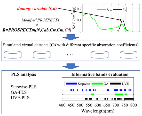
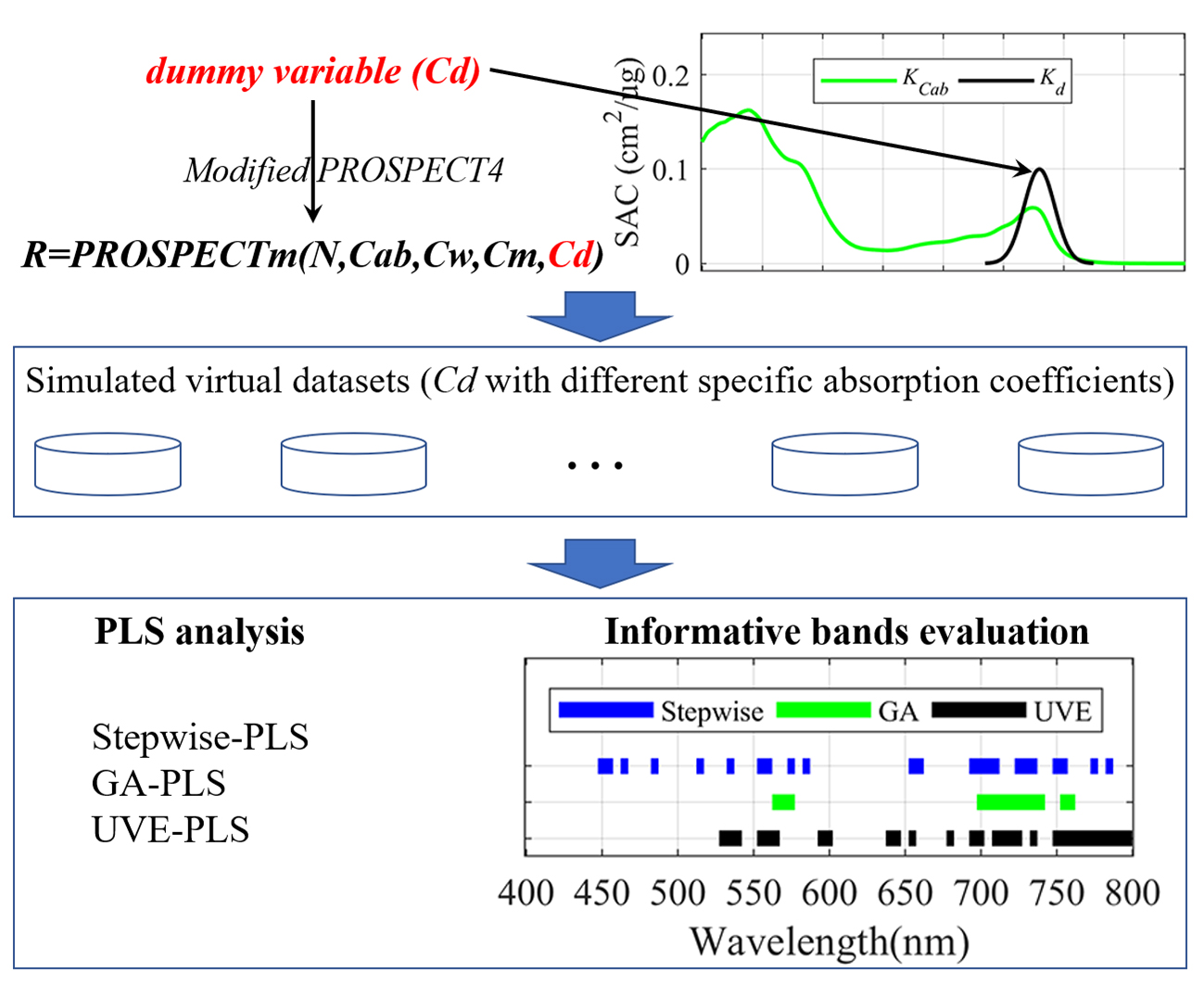
:Partial least squares (PLS) regression models are widely applied in spectroscopy to estimate biochemical components through hyperspectral reflected information. To build PLS regression models based on informative spectral bands, rather than strongly collinear bands contained in the full spectrum, is essential for upholding the performance of models. Yet no consensus has ever been reached on how to select informative bands, even though many techniques have been proposed for estimating plant properties using the vast array of hyperspectral reflectance. In this study, we designed a series of virtual experiments by introducing a dummy variable (Cd) with convertible specific absorption coefficients (SAC) into the well-accepted leaf reflectance PROSPECT-4 model for evaluating popularly adopted informative bands selection techniques, including stepwise-PLS, genetic algorithms PLS (GA-PLS) and PLS with uninformative variable elimination (UVE-PLS). Such virtual experiments have clearly defined responsible wavelength regions related to the dummy input variable, providing objective criteria for model evaluation. Results indicated that although all three techniques examined may estimate leaf biochemical contents efficiently, in most cases the selected bands, unfortunately, did not exactly match known absorption features, casting doubts on their general applicability. The GA-PLS approach was comparatively more efficient at accurately locating the informative bands (with physical and biochemical mechanisms) for estimating leaf biochemical properties and is, therefore, recommended for further applications. Through this study, we have provided objective evaluations of the potential of PLS regressions, which should help to understand the pros and cons of PLS regression models for estimating vegetation biochemical parameters.
1. Introduction
Partial least squares (PLS) regression, a traditional linear statistical approach [1], is suitable for analyzing multi-collinear spectral datasets and has the ability to make full use of redundant information [2]. To date, various PLS regression (PLSR) models that have been built to estimate plant biochemical and biophysical variables from hyperspectral remote sensing data [3,4,5,6,7,8,9,10], have remained oblivious to the serious collinearity among different bands. Many researchers have claimed the superiority of PLSR over other regression techniques, including vegetation indices, multiple linear regression, stepwise regression, and principal component regression [4,11,12,13,14,15]. However, previous studies have also revealed that the wavelengths used by PLSR models may contain irrelevant information, which would dramatically reduce the models’ generality and predictive ability [16].
Due to the high collinearity or correlations among the reflectance values at different bands, one of the inherent challenges with the PLS approach, with so many wavelength variables, is the risk of overfitting [2]. It has been demonstrated in many previous studies, both experimentally and theoretically, that the performance of PLSR can be tremendously improved if only informative variables are included in the model [2,16,17,18,19,20]. After those variables which contain irrelevant or redundant information are removed, the robustness of the calibration models can be enhanced [21].
So far, a number of statistical techniques have been proposed to select informative spectral bands (or eliminate uninformative bands) for PLSR analyses [2,22]. For instance, variable selection based on: (1) PLS regression coefficients, e.g., PLS with uninformative variable elimination (UVE-PLS) [23,24], PLS regression combined with a sure independence screening procedure (PLSSIS) [16]; (2) statistical significance of model prediction, e.g., PLS with stepwise regression variable selection (stepwise-PLS) [19,25,26], exhaustive band combination search [3]; and (3), biological evolution theory and natural selection, e.g., genetic algorithms PLS (GA-PLS) [27].
However, despite so many techniques having been proposed, no consensus has yet been reached on how to select informative bands for plant properties estimation among the vast array of hyperspectral remote sensing data, making physical and biochemical interpretations of selected informative bands nearly impossible. Taking chlorophyll as an example, diverse bands have currently been proposed using PLS regressions. For instance, the bands of 405, 435, 470, 525, 570, 630, 645, 660, 700, and 780 nm for chlorophyll a and the bands of 405, 435, 470, 505, 525, 570, 590, 645, 660, and 700 nm for chlorophyll b content in soybean leaves were used in [10], as well as the bands of 503, 551, 690, 717, and 770 nm for total chlorophyll of pepper leaves in [9]. In contrast, the bands of 460, 470, 480, 530, 540, 550, 730, 740, and 750 nm for chlorophyll were used in [3]. Furthermore, our recent research results on informative spectral band selection for PLS models to estimate foliar chlorophyll content in four independent field-measured datasets, clearly revealed that the bands finally picked-up were inconsistent among the four different datasets [28]. Thus, a selection mechanism-based model with informative bands remains a critical problem in ensuring the robustness of PLSR.
Clearly, the inconsistency of the reported informative bands resulted primarily from the particularity or sample size limitations of these studies. The success of statistical methods to assess plant parameters from optical properties also greatly depends upon the quality of the datasets used. Models calibrated based on small or specialized datasets often perform poorly when applied to other datasets [6]. Another important point worth mentioning is that chlorophyll absorbs light throughout the whole spectral region of 400–750 nm [29], making it difficult to judge the informativeness of one particular band. Furthermore, because of the absorption overlap with other pigments (e.g., carotenoids, anthocyanin), it is difficult to consider which variables are responsible for the property of interest from the aspect of model interpretation [16].
To address this problem, we have generated a rather comprehensive dataset for calibrating PLSR models, based on so-called hybrid methods, combining physically-based models to develop statistical models [6,30,31,32]. The physical law-based radiative transfer models are not only available to generate datasets containing numerous samples [6,30,31,32,33,34], but are also important tools for revealing the underlying relationships between vegetation biochemical parameters and reflectance in a more systematic way [35].
To assess the performance of different variable selection/elimination approaches to locate the optimal wavelengths, we designed virtual experiments based on the well-accepted leaf reflectance model PROSPECT-4 [29,36] by introducing a dummy variable (Cd) with convertible specific absorption coefficients (SAC) into the original version. The modified model enables us to identify the responsible wavelength regions related to the dummy input variable and will, therefore, provide an objective evaluation of the physical and biochemical mechanisms of informative bands later selected by different approaches. This is achieved through a series of virtual datasets based on the modified PROSPECT-4 model by changing the SAC (location, intensity, width) of Cd, providing objective criteria for distinguishing mechanism-based informative bands. Based on these simulated datasets, we established PLSR models with bands selected by three commonly applied techniques, including: (1) the model prediction-based stepwise regression method (stepwise-PLS); (2) biological evolution theory-based genetic algorithms (GA-PLS); and (3) PLS regression coefficients-based uninformative variable elimination method (UVE-PLS). By comparing the bands selected with previously defined absorption features of Cd, we were able to evaluate the efficiency of each method in locating the mechanism-holding wavelengths. We aimed to provide a comprehensive evaluation of the informativeness of selected bands in PLS models for a better understanding of PLS regression performance for vegetation biochemical parameters estimation.
2. Materials and Methods
2.1. Experimental Designs and Data for Calibration and Validation
2.1.1. PROSPECT-4 Modification
The PROSPECT-4 model is a well-accepted leaf-scale radiative transfer model, which considers the leaf as a succession of absorbing layers and simulates leaf hemispherical reflectance and transmittance between 400 and 2500 nm with a 1-nm step, as a function of the leaf structure parameter (N), leaf chlorophyll content (Cab, µg/cm2), leaf water content (Cw, g/cm2) and leaf dry matter content (Cm, g/cm2) [29,30,31]. Inside the model, the reflectance is calculated using the specific absorption coefficient, K, of each component, which depends on the wavelength [31]. The model has been widely applied in numerous studies [6,30,31,32,33,34].
In this study, we added a dummy variable (Cd) into the original PROSPECT-4 model. By tweaking different SACs of Cd, we could, therefore, theoretically compare the properties of the selected wavelengths from different variable selection/elimination approaches for PLSR.
With the artificially added dummy variable Cd and its specific SACs, the total absorption coefficient at each wavelength λ (k(λ)) for one layer in the modified PROSPECT-4 model was calculated as follows:
where N is the leaf structure parameter, Kcab(λ), Kw(λ), and Km(λ) are the specific absorption coefficients at wavelength λ of total chlorophyll, water, and dry matter, respectively, and which are already included in the original PROSPECT-4. Kd(λ) is the specific absorption coefficient of the artificially added dummy variable Cd. The SACs of the dummy variable (Kd) were generated using the following Gaussian function:
where e is Euler’s number, a is the height of the absorption peak, b is the wavelength of the absorption peak, and c is the standard deviation which controls the width of absorption bands, whose value was generated from the predetermined half-width (W) [37]:
The absorption of Cd was limited to the wavelength region between b−1.5×W and b+1.5×W. The Kd values beyond this wavelength region were assigned to 0.
2.1.2. Experimental Design and Database Generation
Various SACs of Cd, with different combinations of locations of absorption peak, peak values, and half-widths, were used to produce different specific absorption coefficients. For simplification, we set the central wavelengths of the absorption peaks at 450 nm, 550 nm, and 680 nm, corresponding to the absorption peak of chlorophyll within the blue region (450 nm), the minimum absorption of chlorophyll within the green region (550 nm), as well as the absorption peak of chlorophyll within the red region (680 nm) [29,38]. Such treatments should have covered most cases for biochemical components under the background of chlorophyll, which shaped the basic reflectance pattern within the wavelength domain of 400 to 800 nm. Furthermore, the absorption peak values of Cd were set to vary from 0.02, 0.04, 0.06, 0.1, 0.2 to 0.3 cm2/μg, while the half-widths were set at levels of 10 nm, 30 nm, 50 nm, respectively.
For each combination of absorption peak location, absorption peak value and half-width, a database composed of 500 simulated leaf reflectance spectra with the modified PROSPECT-4 model, using parameters generated according to their actual distributions as all vegetation types contained in the Leaf Optical Properties Experiment (LOPEX) database [39], was built up. Based on the means (1.67 for N, 47.28 ug/cm2 for Cab, 0.0114 g/cm2 for Cw, and 0.0054 g/cm2 for Cm) and standard deviations (0.33 for N, 17.30 ug/cm2 for Cab, 0.0069 g/cm2 for Cw, and 0.0025 g/cm2 for Cm) calculated from the LOPEX dataset, the parameters of N, Cab, and Cm were randomly selected following a normal distribution, while the values of Cw followed a log-normal distribution [6]. For the newly added dummy variable Cd, we allocated a normal distribution with mean and standard deviation values of 11.83 ug/cm2 and 4.32 ug/cm2 (with the assumption that the measured Cd values were 0.25×Cab), respectively.
2.2. PLS Analysis
For computational efficiency, we limited the spectral range to within the domain of 400-800 nm, covering the spectral regions of chlorophyll and dummy variable absorption [31,40,41,42,43]. We further limited the resolution at 5 nm (resampled with a moving average filter) for the same reason. Three different commonly applied variable selection/elimination approaches (stepwise, genetic algorithms and uninformative variable elimination) were coupled with PLS models to compare their optimality for locating informative bands for leaf biochemical parameter estimation.
2.2.1. Stepwise-PLS
Stepwise selection is the simplest and most pragmatic search method, in which subsequent variables are selected stepwise by their capability to improve a multiple linear regression (MLR) model [26,44,45,46]. Stepwise regression is a systematic method for adding or removing variables from a multilinear model based on their statistical significance in a regression. In this method, the P value of an F-statistic is computed to test models with and without a potential variable at each step [47]. In this study, the bidirectional elimination approach, a combination of forward selection and backward elimination, was applied for stepwise regression [48]. The maximum P values for a spectral band to be included or removed were defined as 0.05 and 0.10, respectively.
2.2.2. GA-PLS
Unlike statistical significance-based variable selection used in stepwise selection, genetic algorithms (GA) are developed on the basis of biological evolution theory and natural selection [17,49], and have significant effects on the band selection of the PLS model [50,51,52]. Following [22], the main steps of GA-PLS include:
- Forming an initial population of variable sets randomly;
- Fitting a PLS regression model to each variable set, and then evaluating the performance with leave-one-out cross-validation;
- Selecting a collection of variable sets with higher performance to survive until the next “generation”;
- Generating new variable sets by crossover (50% probability in this study) and mutation (1% probability in this study) for each variable;
- Using the surviving and modified variable sets as inputs in step 2, and repeating steps 2–5 for a preset number of times (200 in this study).
2.2.3. Uninformative Variable Elimination with PLS (UVE-PLS)
The UVE-PLS approach was proposed in [23] using a reliability criterion calculated from the PLS regression coefficients to evaluate the informativeness of each variable. The regression coefficient matrix was calculated through a leave-one-out validation, and the reliability criterion, cλ, of band λ was determined by the ratio of the mean value of the regression coefficient, bλ. and its standard deviation std(bλ) as:
2.2.4. Evaluation of Different PLSR Models
The commonly used statistical criteria, the normalized root-mean-square error (NRMSE, which is the RMSE normalized using the mean value) and the coefficient of determination (R2), were used in this study to evaluate the estimation accuracy of the PLSR models. However, as the bands involved in different PLSR models could vary, the corrected Akaike information criterion (AICc) [53,54] was instead used as the premier criterion to evaluate the goodness-of-fit of different PLSR models.
3. Results
3.1. Informative Bands Selected for PLSR Models under Different Absorption Peak Locations
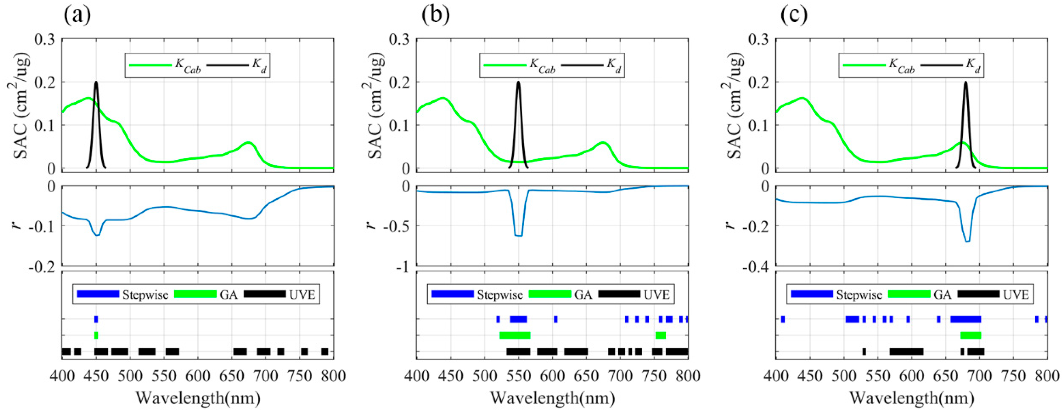
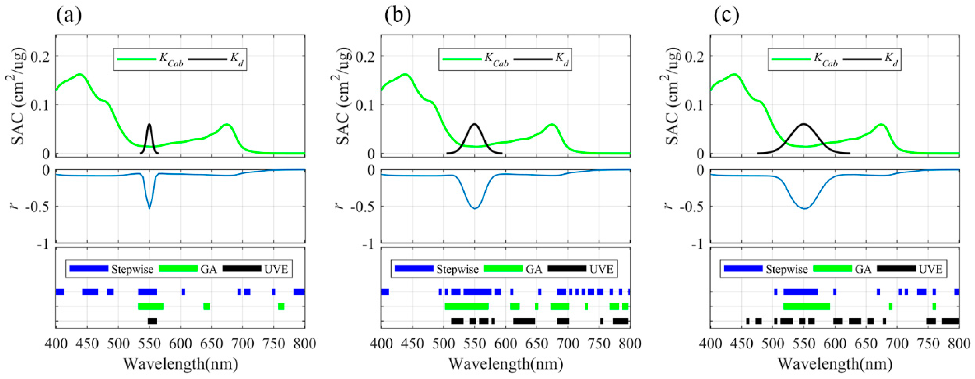
To illustrate the performance of different variable selection/elimination approaches for locating the informative bands, we have specifically presented the bands selected for Cd estimation under distinct absorption peak locations with a narrow absorption half-width (10 nm) in Figure 1. This specific dataset used for PLSR model calibration was generated using a fixed absorption peak intensity of 0.20 cm2/ug, which is higher than the SAC peaks of Cab throughout the spectral region of 400–800 nm.
Results clearly indicated that when the absorption peak of Cd was located within the domain with strong chlorophyll absorption (450 nm), the correlation coefficient (r) of Cd and reflectance varied from 0.00 to −0.12 within the wavelength domain of 400 to 800 nm being examined, and its global extremum appeared at 450 nm. It is worthy of note that the informative bands identified by both stepwise-PLS and GA-PLS approaches (450 nm) fell exactly within the wavelength domain that was affected by Cd (435–465 nm). By comparison, many non-affected bands of Cd (beyond the domain of 435 to 465) were also picked up by the UVE-PLS method, besides the identified informative bands of 450 to 465 nm.
Alternatively, when the absorption peak of Cd was located near 550 nm, a domain with gentle chlorophyll absorption, the correlation coefficient (r) between Cd and reflectance even reached −0.62 around 550 nm. Furthermore, the informative bands within the absorption region of Cd were successfully captured by all the three different approaches. Unfortunately, several redundant, apparently non-affected, bands within 700–800 nm were also included. Furthermore, bands within 580–700 nm, which were also beyond the affected domain, were used in the UVE-PLS models.
In the case of the absorption peak location of Cd being fixed to 680 nm, the extremum of the correlation coefficient (r) between Cd and reflectance appeared at 680 nm (with a value of −0.28). Again, the informative bands affected by Cd (665–695 nm) were captured in all the PLS models. However, besides these Cd affected bands, the stepwise-PLS, and UVE-PLS models also used non-affected bands within 400–650 nm.
3.2. Informative Bands Selected for PLSR Models under Different Absorption Intensities
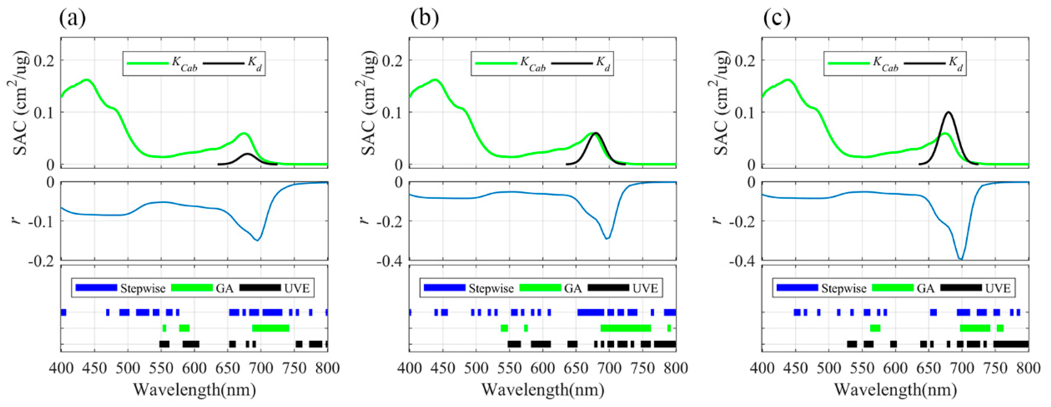
The informative bands involved in the PLSR models also varied with the absorption intensity of Cd, as illustrated in Figure 2, which shows the informative bands picked up by different approaches under varying absorption intensities of Cd. Here we have only presented the cases when the absorption peak location of Cd was set to 680 nm, which is around the absorption peak of chlorophyll within the red region. The absorption half-width of Cd was set to 30 nm in the meantime.
Results showed that the extrema of the correlation coefficient of Cd and reflectance were located around the peaks of Kd/KCab (the ratio between the SAC of the artificially added dummy variable and the SAC of chlorophyll). The highest correlation coefficient of Cd and reflectance was −0.15 at 695 nm when the absorption intensity of Cd set to 0.02 cm2/ug, while it was -0.29 at the same location (695 nm) when the absorption intensity of the Cd was set to 0.06 cm2/ug, and further improved to −0.39 at 700 nm when the absorption intensity of the Cd was set to 0.10 cm2/ug.
Although more or less informative bands within the absorption regions of Cd, and thus with physiochemical mechanisms, were selected by all the variable selection/elimination approaches examined, a large set of bands (with correlation coefficient (r) values for Cd and reflectance of < 0.10) out of the wavelengths affected by Cd, and thus lacking physiochemical mechanisms, were also used in the PLS models, especially the stepwise-PLS and UVE-PLS models.
3.3. Informative Bands Selected for PLSR Models under Different Absorption Half-Widths
We also investigated the selection results for Cd with different absorption half-widths of 10 nm, 30 nm, and 50 nm (Figure 3). Here the absorption peak location of Cd was fixed to 550 nm, with weak disturbance of chlorophyll, and the absorption intensity was set to 0.06 cm2/ug, a value approximating the SAC peak value of chlorophyll in the red region.
The highest correlation coefficients between Cd and reflectance were found at 550 nm, with the same value of −0.53 for all three cases under different absorption half-widths. For Cd with the narrowest absorption half-width (10 nm), the Cd -affected bands were found within the range of 535–563 nm and were involved in all the stepwise-PLS, GA-PLS and UVE-PLS models. However, besides these bands that were clearly affected by the dummy variable, all approaches used many more bands that were supposed to lack physiochemical mechanisms. By comparison, the stepwise-PLS models used more non-affected bands than those of the GA-PLS and UVE-PLS models. With the increase of absorption half-widths, broader wavelength regions with high correlation coefficient (r) values were identified, but non-affected bands could not have been eliminated by whichever of the approaches was being examined.
3.4. Statistical Criteria of Different PLSR Models for Estimating Cd
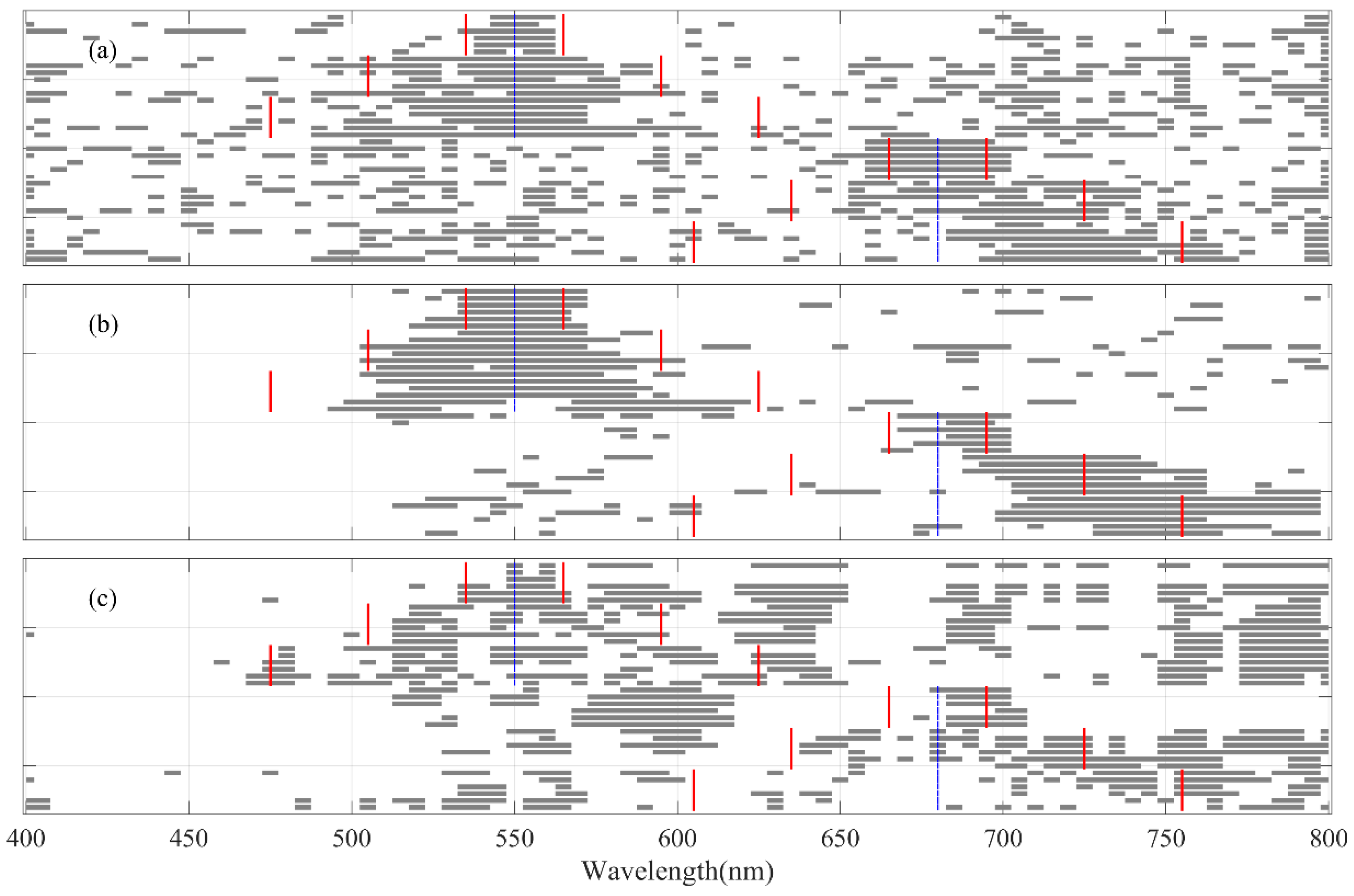
According to the statistical criteria of NRMSE, R2 and AICc, as presented in Table 1, all calibrated PLSR models efficiently estimated Cd in most cases when the absorption peak location of Cd was set to 550 nm or 680 nm, even when the bands selected were not strictly located within the affected bands of Cd. However, when the absorption peak location of Cd was set to 450 nm, because even low contents of Cd are sufficient to saturate absorption due to the strong absorption of chlorophyll within the blue band, calibrated PLS models were far less efficient compared with those cases when the absorption peak locations of Cd were set to 550 nm or 680 nm. Furthermore, when the half-width of Cd was set to broader values, calibrated PLSR models performed better in tracing Cd, as more informative bands were involved in PLSR models.
In comparison, when the absorption peak locations of the dummy variable were set to 550 nm and 680 nm, regardless of the absorption halfwidths and intensities, all calibrated PLSR models efficiently traced Cd according to the statistical criteria of NRMSE and R2.
We further examined the bands involved in these models, and the results are illustrated in Figure 4. It is apparent that a bunch of bands beyond the absorption regions of Cd, and clearly not affected by the dummy variable, were selected by the stepwise-PLS and UVE-PLSR methods for all cases. Compared with stepwise-PLS and UVE-PLS, the bands selected by the GA-PLS method better matched the defined absorption regions of Cd, suggesting that they were more robust and had physiochemical mechanisms. Overall, the results revealed that the GA-PLS method, developed on the basis of biological evolution theory, was more efficient at locating the mechanism-supported informative bands for PLSR estimation of leaf biochemical properties than the other two approaches, stepwise-PLS and UVE-PLS.
4. Discussion
4.1. Collinearity among Reflectance Values
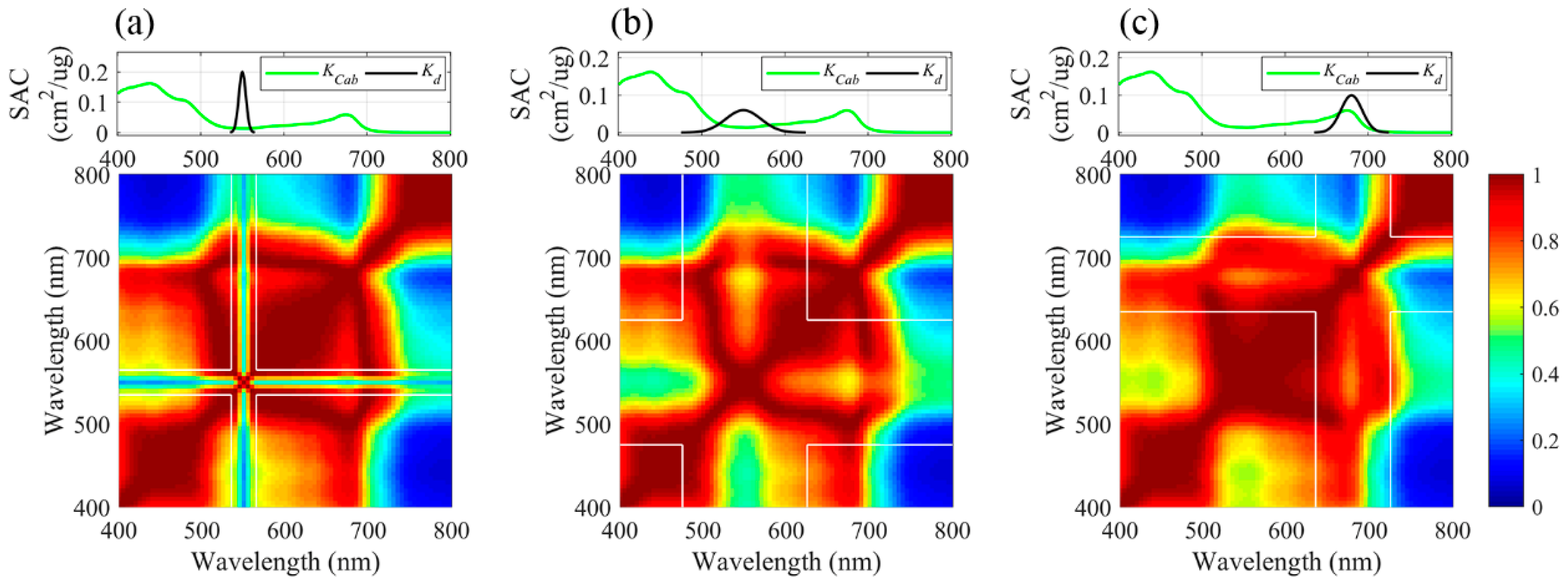
The collinearities among the reflectance bands could cause serious problems in multiple regression, such as instability of estimated coefficients, which make predictions by the regression model poor [2,55,56]. We also hypothesized that the collinearities underly the difficulty data-oriented statistical approaches like PLSR models have in identifying mechanism-based informative bands, leading to so many non-affected bands being involved in the PLSR models for Cd estimation, regardless of the absorption peak locations, intensities and half-widths of Cd. To further illustrate this reason, we investigated all correlations among different bands, as shown in Figure 5.
The correlation patterns shown in Figure 5a used the same data as in Figure 1b. The reflectance values at the absorption peak (550 nm) did not show significant correlations (r < 0.40) with the reflectance values within the bands of 400–515 nm and 625–800 nm. However, the reflectance values around 540 nm and 560 nm were highly correlated (r > 0.60) with those bands throughout the wavelength domain of 465 to 745 nm. The correlation coefficients of the reflectance bands at Cd’s weak absorption bands (540 and 560 nm) and those bands within the range of 685–725 nm were even higher than 0.80.
The correlation coefficient map shown in Figure 5b illustrates the same specific case as in Figure 3c. The correlation coefficients between reflectance at Cd’s absorption peak (550 nm) and bands within the range of 500–740 nm, were all > 0.60. Moreover, the correlation coefficients between reflectance bands around 510 nm (within the absorption band region of Cd) and those within the range of 415–705 nm were even > 0.80, with the highest > 0.95 (the reflectance band at 510 nm and those bands within 585-695 nm).
High correlations between the reflectance at Cd -affected bands and non-affected bands were also identified, as shown in Figure 5c, in which the reflectance bands within the range of 625–685 nm were highly correlated (r > 0.70), with those within the range of 400–700 nm. In addition, the reflectance bands within the range of 690–725 nm were also highly correlated (r > 0.70) with those within the range of 520–620 nm. Furthermore, the correlation coefficients of the reflectance band at 725 nm and bands within the range of 730–800 nm were even > 0.82. Such highly correlated bands (most not caused by the dummy variable, theoretically) are hence getting involved in the PLSR models, especially the stepwise-PLS and UVE-PLS models, and are likely to be the primary reason for these non-affected bands being used in PLSR models.
4.2. Informative Bands Selected by Different Methods for Leaf Biochemical Parameters
Building PLSR models from informative spectral bands, rather than using full bands, could refine the performance of PLS analysis in field spectroscopy [2]. In this study, we investigated three different band selection methods for setting up PLSR models to retrieve Cd, which had clearly defined absorption features. It was apparent, in most cases, that the GA-PLS method outperformed the other two methods in locating the mechanism-based informative bands (i.e., the bands affected by the absorption of the dummy variable in this study).
Stepwise regression is a popular statistical technique for choosing terms to include in a regression model for large data sets [57]. A previous study by Huang et al. (2004) reported that the wavelengths selected by the stepwise regression methods for foliage chemical concentrations estimation were closely related to the known absorption features, in contrast to our results. However, there are several critical issues with stepwise regression, including its inability to cope with redundant dimensions (it deteriorates in the presence of collinearity) and its inability to shrink regression coefficients [58,59]. High dependency or correlations between the reflectance bands, as revealed in this study, make the stepwise approach problematic for locating known absorption features of Cd.
On the other hand, the UVE-PLS is strongly affected by the magnitude of regression coefficients of variables, as it is a method for variable selection based on an analysis of PLS regression coefficients [20]. This method is good at eliminating variables that are irrelevant rather than selection of the best small subset of variables for fitting a model [3,23]. Our results also suggested that several non-affected bands were involved in the UVE-PLS models for Cd estimation. Most likely, an artificially added random matrix might have influenced the model [22].
In contrast, the genetic algorithm (GA) approach had a significant effect in the band optimization selection of the PLS model [17]. However, a simple GA algorithm implementation could only locate near-optimal solutions, while failing in most cases to converge on the optimal solution [60,61]. A previous study on estimating pasture mass and quality from field hyperspectral data with the GA-PLS model suggested that although the selected bands did not exactly match published absorption peaks of specific materials, most were within the 30-nm vicinity of the peaks [2]. Similar results were obtained in our study.
4.3. Performance of PLS Models for Field-Measured Datasets
As the study reported here was mainly based on simulation data resulting from virtual experiments, a previous study by Jin and Wang [28], which evaluated the performance of different informative band selection techniques for PLS towards better estimation of leaf chlorophyll contents of various species from reflected hyperspectral information, should provide a good comparison. The study was based on four field-measured datasets containing a total of 598 leaf samples from various species. It is reported that the calibrated stepwise-PLS and GA-PLS models can estimate the contents of chlorophyll with high accuracy (R2 > 0.70) at different spectral resolutions (1–50 nm). Taking a spectral resolution of 10 nm as an example, which is a common resolution approximate to the specification of several existing hyperspectral sensors such as Hyperion, AVIRIS, MARTE VNIR imaging spectrometer and CRISM [62,63,64], the best estimation of the content of chlorophyll could reach an R2 of 0.77. However, some discrepancies in the informative bands used by the stepwise-PLS and GA-PLS models were noted. The bands selected by the GA-PLS method were within the ranges of 540–580 and 720–780 nm, while bands of 400, 630, 700–710, 730–740, 760 and 780 nm were selected by the stepwise-PLS method. In a similar work by Kira et al. (2015), bands of 460–480, 530–550 and 730–750 nm were suggested as informative bands of the PLS model for chlorophyll estimation, based on their field measured dataset which contained 90 leaves from three species (maple, chestnut, and beech), in which the two band regions of 530–550 and 730–750 nm were in good agreement with the band regions selected by GA-PLS. Furthermore, the number of hyperspectral indices for chlorophyll estimation reviewed in le Maire et al. (2004) and Main et al. (2011) also suggested that wavelengths of 550 nm, around 750 nm, and 800 nm were the premier wavelengths used in published chlorophyll indices [31,43]. Thus, for field-measured datasets, the GA-PLS method was proven efficient for locating the informative bands for estimating leaf biochemical parameters.
4.4. Advantages and Disadvantages of PLS Models for estimating Leaf Biochemical Contents
PLSR has proven to be a very versatile method for multivariate data analysis, especially for high-dimensional data, among diverse research fields such as bioinformatics, machine learning and chemometrics [22]. Previous studies on retrieving various plant characteristics from spectral data have also demonstrated that PLS outperformed other regression techniques (e.g., vegetation indices, multiple linear regression, stepwise regression, and principal component regression) based on statistical criteria such as normalized root-mean-square error (NRMSE) or/and the coefficient of determination (R2) [4,11,12,13,14,15]. However, on the other hand, we must realize that the PLSR models usually involved more bands when using high-dimensional hyperspectral remote sensing data, leading to a high possibility of overfitting. A previous study on canopy nitrogen content demonstrated that the predictive ability of a two-band based index was comparable to that of a PLSR model using all the hyperspectral data [65]. Moreover, another study suggested that vegetation indices used fewer bands than a PLSR model (three versus four), but was more capable of detecting chlorophyll content during the shooting stage and trumpet stage [66]. Research on retrieving leaf area index and leaf chlorophyll concentration at different growth stages of winter wheat concluded that the narrow-band indices were optimal, and a PLSR model, using the information from all wavelengths in the hyperspectral region, did not show any significant improvement [5]. Thus, there is a high risk of overfitting using PLSR with so many bands (especially using all hyperspectral bands) [46], which may be the reason for the data-oriented PLSR models performing worse on retrieving plant characteristics at different growth stages than indices based on fewer bands.
Furthermore, although PLS models could estimate leaf biochemical contents with hyperspectral reflectance efficiently, the selected bands based on popular data-oriented methods, could not exactly match known absorption features to ensure all bands used were mechanism-based. Thus, the selection of informative bands for PLS models to reduce the risk of overfitting remains a great challenge when applying PLSR for plant biochemical content estimation from high-dimensional reflectance. Overall, based on the virtual analysis carried out in this study, we concluded that the GA-PLS method developed on the basis of biological evolution theory located the mechanism-based wavelengths for PLS estimation of leaf biochemical properties more efficiently and reliably than other band selection/elimination methods.
5. Conclusions
To evaluate the efficiency of band selection methods for PLS models and the ability to locate physiochemical mechanism-based informative bands, we conducted a series of virtual analyses based on the modified PROSPECT-4 model. Although the PLSR models could estimate leaf biochemical contents from hyperspectral reflectance efficiently, the selected bands, unfortunately, did not exactly match known absorption features, resulting in poor robustness and generality of the models. The collinearities among the reflectance values at different bands may be the primary reason for including non-affected bands into PLSR models, and this will be treated explicitly in future studies. In general, the GA-PLS method, developed on the basis of biological evolution theory, was more efficient at locating the physicochemical mechanism-based, informative bands. Results obtained in this study should help to lay a basis for better understanding of PLS regression performance in retrieving vegetation biochemical parameters.
Author Contributions
Conceptualization, Q.W.; Methodology, J.J.; Writing, J.J. and Q.W.
Funding
This study was partially supported by the JSPS projects (Grant No. 16H04933 and Grant No. 16KK0170).
Conflicts of Interest
The authors declare no conflicts of interest.
References
- Verrelst, J.; Camps-Valls, G.; Muñoz-Marí, J.; Rivera, J.P.; Veroustraete, F.; Clevers, J.G.P.W.; Moreno, J. Optical remote sensing and the retrieval of terrestrial vegetation bio-geophysical properties—A review. ISPRS J. Photogramm. Remote Sens. 2015, 108, 273–290. [Google Scholar] [CrossRef]
- Kawamura, K.; Watanabe, N.; Sakanoue, S.; Lee, H.J.; Inoue, Y.; Odagawa, S. Testing genetic algorithm as a tool to select relevant wavebands from field hyperspectral data for estimating pasture mass and quality in a mixed sown pasture using partial least squares regression. Grassl. Sci. 2010, 56, 205–216. [Google Scholar] [CrossRef]
- Kira, O.; Linker, R.; Gitelson, A. Non-destructive estimation of foliar chlorophyll and carotenoid contents: Focus on informative spectral bands. Int. J. Appl. Earth Obs. Geoinf. 2015, 38, 251–260. [Google Scholar] [CrossRef]
- Yi, Q.; Jiapaer, G.; Chen, J.; Bao, A.; Wang, F. Different units of measurement of carotenoids estimation in cotton using hyperspectral indices and partial least square regression. ISPRS J. Photogramm. Remote Sens. 2014, 91, 72–84. [Google Scholar] [CrossRef]
- Hansen, P.M.; Schjoerring, J.K. Reflectance measurement of canopy biomass and nitrogen status in wheat crops using normalized difference vegetation indices and partial least squares regression. Remote Sens. Environ. 2003, 86, 542–553. [Google Scholar] [CrossRef]
- Féret, J.-B.; François, C.; Gitelson, A.; Asner, G.P.; Barry, K.M.; Panigada, C.; Richardson, A.D.; Jacquemoud, S. Optimizing spectral indices and chemometric analysis of leaf chemical properties using radiative transfer modeling. Remote Sens. Environ. 2011, 115, 2742–2750. [Google Scholar] [CrossRef] [Green Version]
- Yu, K.; Lenz-Wiedemann, V.; Chen, X.; Bareth, G. Estimating leaf chlorophyll of barley at different growth stages using spectral indices to reduce soil background and canopy structure effects. ISPRS J. Photogramm. Remote Sens. 2014, 97, 58–77. [Google Scholar] [CrossRef]
- Yu, K.; Gnyp, M.L.; Gao, L.; Miao, Y.; Chen, X.; Bareth, G. Estimate Leaf Chlorophyll of Rice Using Reflectance Indices and Partial Least Squares. Photogramm. Fernerkund. Geoinf. 2015, 2015, 45–54. [Google Scholar] [CrossRef]
- Yu, K.-Q.; Zhao, Y.-R.; Zhu, F.-L.; Li, X.-L.; He, Y. Mapping of Chlorophyll and SPAD Distribution in Pepper Leaves During Leaf Senescence Using Visible and Near-Infrared Hyperspectral Imaging. Trans. ASABE 2016, 59, 13. [Google Scholar] [CrossRef]
- Pan, W.-J.; Wang, X.; Deng, Y.-R.; Li, J.-H.; Chen, W.; Chiang, J.Y.; Yang, J.-B.; Zheng, L. Nondestructive and intuitive determination of circadian chlorophyll rhythms in soybean leaves using multispectral imaging. Sci. Rep. 2015, 5, 11108. [Google Scholar] [CrossRef] [Green Version]
- Huang, Z.; Turner, B.J.; Dury, S.J.; Wallis, I.R.; Foley, W.J. Estimating foliage nitrogen concentration from HYMAP data using continuum removal analysis. Remote Sens. Environ. 2004, 93, 18–29. [Google Scholar] [CrossRef]
- Darvishzadeh, R.; Skidmore, A.; Schlerf, M.; Atzberger, C.; Corsi, F.; Cho, M. LAI and chlorophyll estimation for a heterogeneous grassland using hyperspectral measurements. ISPRS J. Photogramm. Remote Sens. 2008, 63, 409–426. [Google Scholar] [CrossRef]
- Atzberger, C.; Guérif, M.; Baret, F.; Werner, W. Comparative analysis of three chemometric techniques for the spectroradiometric assessment of canopy chlorophyll content in winter wheat. Comput. Electron. Agric. 2010, 73, 165–173. [Google Scholar] [CrossRef]
- Ryu, C.; Suguri, M.; Umeda, M. Multivariate analysis of nitrogen content for rice at the heading stage using reflectance of airborne hyperspectral remote sensing. Field Crop. Res. 2011, 122, 214–224. [Google Scholar] [CrossRef] [Green Version]
- Fu, Y.; Yang, G.; Wang, J.; Song, X.; Feng, H. Winter wheat biomass estimation based on spectral indices, band depth analysis and partial least squares regression using hyperspectral measurements. Comput. Electron. Agric. 2014, 100, 51–59. [Google Scholar] [CrossRef]
- Huang, X.; Xu, Q.-S.; Liang, Y.-Z. PLS regression based on sure independence screening for multivariate calibration. Anal. Methods 2012, 4, 2815–2821. [Google Scholar] [CrossRef]
- Wu, Q.; Wang, J.; Wang, C.; Xu, T. Study on the optimal algorithm prediction of corn leaf component information based on hyperspectral imaging. Infrared Phys. Technol. 2016, 78, 66–71. [Google Scholar] [CrossRef]
- Chen, H.; Chen, T.; Zhang, Z.; Liu, G. Variable Selection Using Adaptive Band Clustering and Physarum Network. Algorithms 2017, 10, 73. [Google Scholar] [CrossRef]
- Wang, Z.; Kawamura, K.; Sakuno, Y.; Fan, X.; Gong, Z.; Lim, J. Retrieval of Chlorophyll-a and Total Suspended Solids Using Iterative Stepwise Elimination Partial Least Squares (ISE-PLS) Regression Based on Field Hyperspectral Measurements in Irrigation Ponds in Higashihiroshima, Japan. Remote Sens. 2017, 9, 264. [Google Scholar] [CrossRef]
- Wang, Z.X.; He, Q.; Wang, J. Comparison of different variable selection methods for partial least squares soft sensor development. In Proceedings of the 2014 American Control Conference, Portland, OR, USA, 4–6 June 2014; pp. 3116–3121. [Google Scholar]
- De Groot, P.J.; Swierenga, H.; Postma, G.J.; Melssen, W.J.; Buydens, L.M.C. Effect on the Partial Least-Squares Prediction of Yarn Properties Combining Raman and Infrared Measurements and Applying Wavelength Selection. Appl. Spectrosc. 2003, 57, 642–648. [Google Scholar] [CrossRef]
- Mehmood, T.; Liland, K.H.; Snipen, L.; Sæbø, S. A review of variable selection methods in Partial Least Squares Regression. Chemom. Intell. Lab. Syst. 2012, 118, 62–69. [Google Scholar] [CrossRef]
- Centner, V.; Massart, D.-L.; de Noord, O.E.; de Jong, S.; Vandeginste, B.M.; Sterna, C. Elimination of Uninformative Variables for Multivariate Calibration. Anal. Chem. 1996, 68, 3851–3858. [Google Scholar] [CrossRef] [PubMed]
- Cai, W.; Li, Y.; Shao, X. A variable selection method based on uninformative variable elimination for multivariate calibration of near-infrared spectra. Chemom. Intell. Lab. Syst. 2008, 90, 188–194. [Google Scholar] [CrossRef]
- Fung, T.; Yan Ma, H.F.; Siu, W.L. Band Selection Using Hyperspectral Data of Subtropical Tree Species. Geocarto Int. 2003, 18, 3–11. [Google Scholar] [CrossRef]
- Schmitt, N.; Ployhart, R.E. Estimates of cross-validity for stepwise regression and with predictor selection. J. Appl. Psychol. 1999, 84, 50. [Google Scholar] [CrossRef]
- Leardi, R.; Boggia, R.; Terrile, M. Genetic algorithms as a strategy for feature selection. J. Chemom. 1992, 6, 267–281. [Google Scholar] [CrossRef]
- Jin, J.; Wang, Q. Selection of informative spectral bands for PLS models to estimate foliar chlorophyll content using hyperspectral reflectance. IEEE Trans. Geosci. Remote Sens. 2018, 1–9. [Google Scholar] [CrossRef]
- Feret, J.-B.; François, C.; Asner, G.P.; Gitelson, A.A.; Martin, R.E.; Bidel, L.P.R.; Ustin, S.L.; le Maire, G.; Jacquemoud, S. PROSPECT-4 and 5: Advances in the leaf optical properties model separating photosynthetic pigments. Remote Sens. Environ. 2008, 112, 3030–3043. [Google Scholar] [CrossRef]
- Le Maire, G.; François, C.; Soudani, K.; Berveiller, D.; Pontailler, J.-Y.; Bréda, N.; Genet, H.; Davi, H.; Dufrêne, E. Calibration and validation of hyperspectral indices for the estimation of broadleaved forest leaf chlorophyll content, leaf mass per area, leaf area index and leaf canopy biomass. Remote Sens. Environ. 2008, 112, 3846–3864. [Google Scholar] [CrossRef]
- Le Maire, G.; François, C.; Dufrêne, E. Towards universal broad leaf chlorophyll indices using PROSPECT simulated database and hyperspectral reflectance measurements. Remote Sens. Environ. 2004, 89, 1–28. [Google Scholar] [CrossRef]
- Wang, Q.; Li, P. Identification of robust hyperspectral indices on forest leaf water content using PROSPECT simulated dataset and field reflectance measurements. Hydrol. Process. 2012, 26, 1230–1241. [Google Scholar] [CrossRef]
- Li, P.; Wang, Q. Retrieval of Leaf Biochemical Parameters Using PROSPECT Inversion: A New Approach for Alleviating Ill-Posed Problems. IEEE Trans. Geosci. Remote Sens. 2011, 49, 2499–2506. [Google Scholar] [CrossRef]
- Qiu, F.; Chen, J.M.; Ju, W.; Wang, J.; Zhang, Q.; Fang, M. Improving the PROSPECT Model to Consider Anisotropic Scattering of Leaf Internal Materials and Its Use for Retrieving Leaf Biomass in Fresh Leaves. IEEE Trans. Geosci. Remote Sens. 2018, 1–18. [Google Scholar] [CrossRef]
- Jin, J.; Wang, Q. Informative bands used by efficient hyperspectral indices to predict leaf biochemical contents are determined by their relative absorptions. Int. J. Appl. Earth Obs. Geoinf. 2018, 73, 616–626. [Google Scholar] [CrossRef]
- Jacquemoud, S.; Baret, F. PROSPECT: A model of leaf optical properties spectra. Remote Sens. Environ. 1990, 34, 75–91. [Google Scholar] [CrossRef]
- Tsai, F.; Philpot, W. Derivative Analysis of Hyperspectral Data. Remote Sens. Environ. 1998, 66, 41–51. [Google Scholar] [CrossRef]
- Eng, D.; Baranoski, G.V.G. The Application of Photoacoustic Absorption Spectral Data to the Modeling of Leaf Optical Properties in the Visible Range. IEEE Trans. Geosci. Remote Sens. 2007, 45, 4077–4086. [Google Scholar] [CrossRef]
- Hosgood, B.; Jacquemoud, S.; Andreoli, G.; Verdebout, J.; Pedrini, G.; Schmuck, G. Leaf Optical Properties Experiment 93 (LOPEX93); European Commission—Joint Research Centre EUR 16095 EN: Ispra, Italy, 1994; p. 20. [Google Scholar]
- Anatoly, G.; Alexei, S. Generic Algorithms for Estimating Foliar Pigment Content. Geophys. Res. Lett. 2017, 44, 9293–9298. [Google Scholar] [CrossRef]
- Dian, Y.; Le, Y.; Fang, S.; Xu, Y.; Yao, C.; Liu, G. Influence of Spectral Bandwidth and Position on Chlorophyll Content Retrieval at Leaf and Canopy Levels. J. Indian Soc. Remote Sens. 2016, 44, 583–593. [Google Scholar] [CrossRef]
- Ustin, S.L.; Gitelson, A.A.; Jacquemoud, S.; Schaepman, M.; Asner, G.P.; Gamon, J.A.; Zarco-Tejada, P. Retrieval of foliar information about plant pigment systems from high resolution spectroscopy. Remote Sens. Environ. 2009, 113, S67–S77. [Google Scholar] [CrossRef] [Green Version]
- Main, R.; Cho, M.A.; Mathieu, R.; O’Kennedy, M.M.; Ramoelo, A.; Koch, S. An investigation into robust spectral indices for leaf chlorophyll estimation. ISPRS J. Photogramm. Remote Sens. 2011, 66, 751–761. [Google Scholar] [CrossRef]
- Norgaard, L.; Saudland, A.; Wagner, J.; Nielsen, J.P.; Munck, L.; Engelsen, S.B. Interval Partial Least-Squares Regression (iPLS): A Comparative Chemometric Study with an Example from Near-Infrared Spectroscopy. Appl. Spectrosc. 2000, 54, 413–419. [Google Scholar] [CrossRef]
- Dorigo, W.A.; Zurita-Milla, R.; de Wit, A.J.W.; Brazile, J.; Singh, R.; Schaepman, M.E. A review on reflective remote sensing and data assimilation techniques for enhanced agroecosystem modeling. Int. J. Appl. Earth Obs. Geoinf. 2007, 9, 165–193. [Google Scholar] [CrossRef]
- Andersen, C.M.; Bro, R. Variable selection in regression—A tutorial. J. Chemom. 2010, 24, 728–737. [Google Scholar] [CrossRef]
- Draper, N.R.; Smith, H. Applied Regression Analysis; John Wiley & Sons: Hoboken, NJ, USA, 1998. [Google Scholar]
- Yu, T.; Yu, G.; Li, P.-Y.; Wang, L.J.S. Citation impact prediction for scientific papers using stepwise regression analysis. Scientometrics 2014, 101, 1233–1252. [Google Scholar] [CrossRef]
- Lu, D.M.; Song, K.S.; Li, L.; Liu, D.W.; Li, S.H.; Wang, Y.D.; Wang, Z.M.; Xu, J.P.; Du, J.; Jia, M.M. Training a GA-PLS Model for Chl-a Concentration Estimation over Inland Lake in Northeast China. Procedia Environ. Sci. 2010, 2, 842–851. [Google Scholar] [CrossRef] [Green Version]
- Leardi, R. Application of genetic algorithm–PLS for feature selection in spectral data sets. J. Chemom. 2000, 14, 643–655. [Google Scholar] [CrossRef]
- Leardi, R.; Lupiáñez González, A. Genetic algorithms applied to feature selection in PLS regression: How and when to use them. Chemom. Intell. Lab. Syst. 1998, 41, 195–207. [Google Scholar] [CrossRef]
- Hasegawa, K.; Miyashita, Y.; Funatsu, K. GA Strategy for Variable Selection in QSAR Studies: GA-Based PLS Analysis of Calcium Channel Antagonists. J. Chem. Inf. Comput. Sci. 1997, 37, 306–310. [Google Scholar] [CrossRef]
- McQuarrie, A.D.R.; Tsai, C.-L. Regression and Time Series Model Selection; World Scientific: Singapore, 1998. [Google Scholar]
- Hurvich, C.M.; Tsai, C.-L. Regression and Time Series Model Selection in Small Samples. Biometrika 1989, 76, 297–307. [Google Scholar] [CrossRef]
- Wold, S.; Ruhe, A.; Wold, H.; Dunn, W.J., III. The Collinearity Problem in Linear Regression. The Partial Least Squares (PLS) Approach to Generalized Inverses. SIAM J. Sci. Stat. Comput. 1984, 5, 735–743. [Google Scholar] [CrossRef]
- Chong, I.-G.; Jun, C.-H. Performance of some variable selection methods when multicollinearity is present. Chemom. Intell. Lab. Syst. 2005, 78, 103–112. [Google Scholar] [CrossRef]
- Wang, Y.; Huang, S.; Liu, D.; Wang, B. Research Advance on Band Selection-Based Dimension Reduction of Hyperspectral Remote Sensing Images. In Proceedings of the 2012 2nd International Conference on Remote Sensing, Environment and Transportation Engineering, Nanjing, China, 1–3 June 2012; pp. 1–4. [Google Scholar]
- Ting, J.-A.; D’Souza, A.; Vijayakumar, S.; Schaal, S. Efficient Learning and Feature Selection in High-Dimensional Regression. Neural Comput. 2010, 22, 831–886. [Google Scholar] [CrossRef] [PubMed] [Green Version]
- Tibshirani, R. Regression Shrinkage and Selection via the Lasso. J. R. Stat. Soc. Ser. B (Methodol.) 1996, 58, 267–288. [Google Scholar] [CrossRef]
- Kazarlis, S.A.; Bakirtzis, A.G.; Petridis, V. A genetic algorithm solution to the unit commitment problem. IEEE Trans. Power Syst. 1996, 11, 83–92. [Google Scholar] [CrossRef]
- Yang, J.; Honavar, V. Feature Subset Selection Using a Genetic Algorithm. In Feature Extraction, Construction and Selection: A Data Mining Perspective; Liu, H., Motoda, H., Eds.; Springer: Boston, MA, USA, 1998; pp. 117–136. [Google Scholar] [Green Version]
- Imanishi, J.; Sugimoto, K.; Morimoto, Y. Detecting drought status and LAI of two Quercus species canopies using derivative spectra. Comput. Electron. Agric. 2004, 43, 109–129. [Google Scholar] [CrossRef]
- Brown, A.J.; Sutter, B.; Dunagan, S. The MARTE VNIR Imaging Spectrometer Experiment: Design and Analysis. Astrobiology 2008, 8, 1001–1011. [Google Scholar] [CrossRef] [Green Version]
- Brown, A.J.; Hook, S.J.; Baldridge, A.M.; Crowley, J.K.; Bridges, N.T.; Thomson, B.J.; Marion, G.M.; de Souza Filho, C.R.; Bishop, J.L. Hydrothermal formation of Clay-Carbonate alteration assemblages in the Nili Fossae region of Mars. Earth Planet. Sci. Lett. 2010, 297, 174–182. [Google Scholar] [CrossRef] [Green Version]
- Inoue, Y.; Sakaiya, E.; Zhu, Y.; Takahashi, W. Diagnostic mapping of canopy nitrogen content in rice based on hyperspectral measurements. Remote Sens. Environ. 2012, 126, 210–221. [Google Scholar] [CrossRef]
- Hong, S.; Minzan, L.; Yane, Z.; Yong, Z.; Haihua, W. Detection of Corn Chlorophyll Content Using Canopy Spectral Reflectance. Sens. Lett. 2010, 8, 134–139. [Google Scholar] [CrossRef]
Figure 1.
Bands selected in partial least squares regression (PLSR) models with three different variable selection/elimination approaches to estimate Cd with different absorption peak locations: (a) 450 nm, (b) 550 nm, and (c) 680 nm. The absorption peak intensities (at absorption peaks) and half-widths shown were set to 0.20 cm2/ug and 10 nm, respectively.

Figure 2.
Bands selected in PLSR models with three different variable selection/elimination approaches to estimate Cd with different absorption intensities: (a) 0.02 cm2/ug; (b) 0.06 cm2/ug; and (c) 0.10 cm2/ug. The locations of absorption peak and half-widths shown were set to 680 nm and 30 nm, respectively.

Figure 3.
Bands selected in PLSR models with three different variable selection/elimination approaches to estimate Cd with different absorption half-widths: (a) 10 nm, (b) 30 nm, and (c) 50 nm. The locations of absorption peaks and absorption intensities were set to 550 nm and 0.06 cm2/ug, respectively.

Figure 4.
Bands involved in stepwise-PLS (a), genetic algorithms (GA-PLS) (b), and uninformative variable elimination method (UVE-PLS) (c) models for Cd estimation. The blue lines are the absorption peak locations of Cd (only results of 550 nm and 680 nm are presented). The red lines are the absorption boundaries of Cd. For one fixed absorption peak location and half-width, the selected bands for PLS estimation of Cd with six absorption intensities were in sequence.

Figure 5.
Correlation coefficient maps of reflectance wavelength pairs from datasets simulated with different Cd absorptions. (a) Absorption peak location at 550 nm with absorption peak value of 0.20 cm2/ug and half-width of 10 nm; (b) absorption peak location at 550 nm with absorption peak value of 0.06 cm2/ug and half-width of 50 nm; (c) absorption peak location at 680 nm with absorption peak value of 0.10 cm2/ug and half-width of 30 nm.


Table 1.
Descriptive statistics of the performance of PLSR models calibrated for estimation of Cd with different absorption peak locations, intensities, and half-widths.
Table 1.
Descriptive statistics of the performance of PLSR models calibrated for estimation of Cd with different absorption peak locations, intensities, and half-widths.
| Peak Location | Intensity | Half-Width | Stepwise-PLS | GA-PLS | UVE-PLS | ||||||
|---|---|---|---|---|---|---|---|---|---|---|---|
| NRMSE | R2 | AICc | NRMSE | R2 | AICc | NRMSE | R2 | AICc | |||
| 450 | 0.02 | 10 | 0.35 | 0.02 | 3.88 | 0.35 | 0.01 | 3.90 | 0.34 | 0.11 | 3.85 |
| 450 | 0.02 | 30 | 0.35 | 0.04 | 3.88 | 0.35 | 0.01 | 3.89 | 0.33 | 0.12 | 3.96 |
| 450 | 0.02 | 50 | 0.35 | 0.01 | 3.89 | 0.28 | 0.39 | 3.43 | 0.22 | 0.61 | 3.00 |
| 450 | 0.04 | 10 | 0.35 | 0.02 | 3.88 | 0.35 | 0.01 | 3.91 | 0.34 | 0.07 | 3.90 |
| 450 | 0.04 | 30 | 0.35 | 0.02 | 3.88 | 0.35 | 0.01 | 3.89 | 0.34 | 0.11 | 3.85 |
| 450 | 0.04 | 50 | 0.34 | 0.11 | 3.80 | 0.18 | 0.75 | 2.54 | 0.08 | 0.95 | 0.93 |
| 450 | 0.06 | 10 | 0.35 | 0.02 | 3.88 | 0.36 | 0.01 | 3.90 | 0.35 | 0.03 | 3.89 |
| 450 | 0.06 | 30 | 0.35 | 0.03 | 3.87 | 0.35 | 0.01 | 3.89 | 0.32 | 0.19 | 3.74 |
| 450 | 0.06 | 50 | 0.33 | 0.15 | 3.75 | 0.08 | 0.95 | 0.91 | 0.07 | 0.96 | 0.84 |
| 450 | 0.10 | 10 | 0.35 | 0.01 | 3.89 | 0.36 | 0.01 | 3.90 | 0.34 | 0.06 | 3.90 |
| 450 | 0.10 | 30 | 0.35 | 0.03 | 3.87 | 0.35 | 0.03 | 3.88 | 0.34 | 0.11 | 3.94 |
| 450 | 0.10 | 50 | 0.15 | 0.83 | 2.27 | 0.07 | 0.96 | 0.75 | 0.18 | 0.75 | 2.56 |
| 450 | 0.20 | 10 | 0.35 | 0.02 | 3.88 | 0.35 | 0.02 | 3.88 | 0.34 | 0.06 | 3.99 |
| 450 | 0.20 | 30 | 0.34 | 0.09 | 3.82 | 0.35 | 0.02 | 3.89 | 0.33 | 0.14 | 3.84 |
| 450 | 0.20 | 50 | 0.07 | 0.97 | 0.68 | 0.11 | 0.90 | 1.61 | 0.05 | 0.98 | 0.12 |
| 450 | 0.30 | 10 | 0.34 | 0.08 | 3.83 | 0.35 | 0.01 | 3.88 | 0.35 | 0.03 | 3.99 |
| 450 | 0.30 | 30 | 0.34 | 0.10 | 3.81 | 0.35 | 0.02 | 3.88 | − | − | − |
| 450 | 0.30 | 50 | 0.07 | 0.96 | 0.79 | 0.13 | 0.86 | 1.96 | 0.10 | 0.93 | 1.38 |
| 550 | 0.02 | 10 | 0.10 | 0.92 | 1.42 | 0.06 | 0.97 | 0.54 | 0.18 | 0.74 | 2.66 |
| 550 | 0.02 | 30 | 0.05 | 0.98 | −0.01 | 0.06 | 0.97 | 0.51 | 0.04 | 0.99 | −0.26 |
| 550 | 0.02 | 50 | 0.04 | 0.98 | −0.11 | 0.04 | 0.99 | −0.44 | 0.03 | 0.99 | −0.64 |
| 550 | 0.04 | 10 | 0.09 | 0.94 | 1.17 | 0.07 | 0.96 | 0.68 | 0.22 | 0.63 | 2.92 |
| 550 | 0.04 | 30 | 0.05 | 0.98 | 0.14 | 0.07 | 0.96 | 0.67 | 0.05 | 0.98 | 0.02 |
| 550 | 0.04 | 50 | 0.04 | 0.98 | −0.16 | 0.05 | 0.98 | −0.11 | 0.04 | 0.98 | −0.14 |
| 550 | 0.06 | 10 | 0.06 | 0.97 | 0.42 | 0.07 | 0.96 | 0.78 | 0.22 | 0.63 | 2.92 |
| 550 | 0.06 | 30 | 0.05 | 0.98 | 0.24 | 0.06 | 0.97 | 0.38 | 0.06 | 0.97 | 0.37 |
| 550 | 0.06 | 50 | 0.04 | 0.99 | −0.60 | 0.04 | 0.98 | −0.22 | 0.05 | 0.98 | 0.11 |
| 550 | 0.10 | 10 | 0.07 | 0.96 | 0.78 | 0.08 | 0.95 | 1.01 | 0.10 | 0.92 | 1.50 |
| 550 | 0.10 | 30 | 0.06 | 0.98 | 0.29 | 0.08 | 0.95 | 0.87 | 0.06 | 0.97 | 0.54 |
| 550 | 0.10 | 50 | 0.07 | 0.96 | 0.85 | 0.05 | 0.98 | 0.16 | 0.09 | 0.94 | 1.23 |
| 550 | 0.20 | 10 | 0.08 | 0.94 | 1.09 | 0.09 | 0.93 | 1.26 | 0.08 | 0.95 | 1.14 |
| 550 | 0.20 | 30 | 0.06 | 0.97 | 0.59 | 0.11 | 0.91 | 1.64 | 0.06 | 0.97 | 0.56 |
| 550 | 0.20 | 50 | 0.09 | 0.94 | 1.28 | 0.09 | 0.93 | 1.32 | 0.08 | 0.95 | 1.04 |
| 550 | 0.30 | 10 | 0.10 | 0.92 | 1.43 | 0.09 | 0.93 | 1.24 | 0.08 | 0.94 | 1.14 |
| 550 | 0.30 | 30 | 0.07 | 0.96 | 0.79 | 0.10 | 0.92 | 1.42 | 0.07 | 0.96 | 0.80 |
| 550 | 0.30 | 50 | 0.09 | 0.94 | 1.33 | 0.10 | 0.92 | 1.41 | 0.09 | 0.94 | 1.23 |
| 680 | 0.02 | 10 | 0.12 | 0.88 | 1.80 | 0.20 | 0.69 | 2.79 | 0.13 | 0.86 | 2.01 |
| 680 | 0.02 | 30 | 0.03 | 0.99 | −0.98 | 0.05 | 0.98 | 0.08 | 0.20 | 0.69 | 2.81 |
| 680 | 0.02 | 50 | 0.02 | 1.00 | −2.04 | 0.02 | 1.00 | −1.58 | 0.02 | 1.00 | −1.96 |
| 680 | 0.04 | 10 | 0.15 | 0.82 | 2.35 | 0.28 | 0.39 | 3.41 | 0.15 | 0.83 | 2.21 |
| 680 | 0.04 | 30 | 0.02 | 1.00 | −1.50 | 0.04 | 0.98 | −0.26 | 0.02 | 1.00 | −1.48 |
| 680 | 0.04 | 50 | 0.02 | 1.00 | −1.56 | 0.03 | 0.99 | −1.19 | 0.02 | 1.00 | −2.19 |
| 680 | 0.06 | 10 | 0.10 | 0.93 | 1.40 | 0.20 | 0.70 | 2.74 | 0.15 | 0.82 | 2.27 |
| 680 | 0.06 | 30 | 0.03 | 0.99 | −1.23 | 0.02 | 1.00 | −1.89 | 0.02 | 1.00 | −2.02 |
| 680 | 0.06 | 50 | 0.02 | 1.00 | −1.86 | 0.02 | 1.00 | −1.57 | 0.02 | 1.00 | −1.80 |
| 680 | 0.10 | 10 | 0.13 | 0.87 | 1.94 | 0.20 | 0.69 | 2.74 | 0.35 | 0.02 | 3.92 |
| 680 | 0.10 | 30 | 0.03 | 0.99 | −1.23 | 0.02 | 1.00 | −2.02 | 0.02 | 1.00 | −1.98 |
| 680 | 0.10 | 50 | 0.02 | 1.00 | −1.93 | 0.03 | 0.99 | −1.23 | 0.02 | 1.00 | −2.04 |
| 680 | 0.20 | 10 | 0.08 | 0.95 | 0.91 | 0.26 | 0.48 | 3.26 | 0.13 | 0.87 | 1.91 |
| 680 | 0.20 | 30 | 0.02 | 1.00 | −1.47 | 0.02 | 1.00 | −1.89 | 0.02 | 1.00 | −1.87 |
| 680 | 0.20 | 50 | 0.03 | 0.99 | −1.08 | 0.02 | 1.00 | −1.97 | 0.02 | 1.00 | −1.34 |
| 680 | 0.30 | 10 | 0.10 | 0.92 | 1.52 | 0.25 | 0.52 | 3.18 | 0.15 | 0.82 | 2.27 |
| 680 | 0.30 | 30 | 0.02 | 1.00 | −2.09 | 0.02 | 1.00 | −1.72 | 0.02 | 1.00 | −1.71 |
| 680 | 0.30 | 50 | 0.03 | 0.99 | −0.94 | 0.02 | 1.00 | −2.00 | 0.04 | 0.99 | −0.52 |
© 2019 by the authors. Licensee MDPI, Basel, Switzerland. This article is an open access article distributed under the terms and conditions of the Creative Commons Attribution (CC BY) license (http://creativecommons.org/licenses/by/4.0/).
Share and Cite
MDPI and ACS Style
Jin, J.; Wang, Q. Evaluation of Informative Bands Used in Different PLS Regressions for Estimating Leaf Biochemical Contents from Hyperspectral Reflectance. Remote Sens. 2019, 11, 197. https://0-doi-org.brum.beds.ac.uk/10.3390/rs11020197
AMA Style
Jin J, Wang Q. Evaluation of Informative Bands Used in Different PLS Regressions for Estimating Leaf Biochemical Contents from Hyperspectral Reflectance. Remote Sensing. 2019; 11(2):197. https://0-doi-org.brum.beds.ac.uk/10.3390/rs11020197
Chicago/Turabian StyleJin, Jia, and Quan Wang. 2019. "Evaluation of Informative Bands Used in Different PLS Regressions for Estimating Leaf Biochemical Contents from Hyperspectral Reflectance" Remote Sensing 11, no. 2: 197. https://0-doi-org.brum.beds.ac.uk/10.3390/rs11020197
Note that from the first issue of 2016, this journal uses article numbers instead of page numbers. See further details here.