Statistical Characterization of the Observed Cold Wake Induced by North Atlantic Hurricanes


Environmental Fluid Mechanics, Department of Hydraulic Engineering, Delft University of Technology, Stevinweg 1, Building 23, 2628CN Delft, The Netherlands
*
Author to whom correspondence should be addressed.
Remote Sens. 2019, 11(20), 2368; https://0-doi-org.brum.beds.ac.uk/10.3390/rs11202368
Submission received: 10 September 2019
/
Revised: 30 September 2019
/
Accepted: 5 October 2019
/
Published: 12 October 2019
(This article belongs to the Special Issue Tropical Cyclones Remote Sensing and Data Assimilation)
Abstract
:This work quantifies the magnitude, spatial structure, and temporal evolution of the cold wake left by North Atlantic hurricanes. To this end we composited the sea surface temperature anomalies (SSTA) induced by hurricane observations from 2002 to 2018 derived from the international best track archive for climate stewardship (IBTrACS). Cold wake characteristics were distinguished by a set of hurricane and oceanic properties: Hurricane translation speed and intensity, and the characteristics of the upper ocean stratification represented by two barrier layer metrics: Barrier layer thickness (BLT) and barrier layer potential energy (BLPE). The contribution of the above properties to the amplitude of the cold wake was analyzed individually and in combination. The mean magnitude of the hurricane-induced cooling was of 1.7 °C when all hurricanes without any distinction were considered, and the largest cooling was found for slow-moving, strong hurricanes passing over thinner barrier layers, with a cooling above 3.5 °C with respect to pre-storm sea surface temperature (SST) conditions. On average the cold wake needed about 60 days to disappear and experienced a strong decay in the first 20 days, when the magnitude of the cold wake had decreased by 80%. Differences between the cold wakes yielded by mostly infrared and merged infrared and microwave remote sensed SST data were also evaluated, with an overall relative underestimation of the hurricane-induced cooling of about 0.4 °C for infrared-mostly data.
1. Introduction
Sea surface temperature (SST) plays a major role in the existence and life of a tropical cyclone (TC). It is recognized as one of the most important factors in TC genesis (together with e.g., the existence of a reduced vertical wind shear, environmental vorticity and high relative humidity). In addition, it is thought to be of most relevance in TC strengthening and weakening, although it is still the subject of scientific debate (e.g., [1] and references therein).
The formation of a region with reduced SST in the wake of tropical cyclones (TCs; so-called hurricanes in the Atlantic basin when a TC attains a certain strength) was already known from measurements provided by merchant ships in the 1950s (e.g., [2,3]). However, the first dedicated systematic survey to evaluate the evolution of the SST field after the passage of a TC was published by Leipper [4], who found a reduction of ∼5 °C in the vicinity of the track of hurricane Hilda (1964). Also Hazelworth [5] detected significant cooling near the US Atlantic coast after the passage of ten hurricanes. These measurements, made with buoys and bathythermographs, yielded a mean cooling between and °C. A similar range of cooling was later estimated from satellite-based measurements. Stramma et al. [6] performed a statistical assessment of the cold wake left by some Atlantic hurricanes between 1981 and 1984 (13 in total) using limited SST images provided by the National Oceanic and Atmospheric Administration (NOAA) advanced very high-resolution radiometer (AVHRR) sensor. They found an overall magnitude of SST cooling of °C that lasted from a few days to around two weeks after the passage of the hurricane along its track. One drawback of that study was that for some hurricanes (mainly for the major hurricanes), the authors only had at hand cloud-free images up to 5 days after the passage of the hurricane, hence likely underestimating the cooling. Moreover, they found that the amount of cooling was quite proportional to the hurricane strength, with the maximum localized at around 70 km to the right of the track for fast-moving hurricanes and closer to the center for slower hurricanes. Indeed this rightward bias (in the Northern Hemisphere, leftward in the Southern Hemisphere) had already been mentioned by Jordan [7] and it has been amply confirmed in subsequent observational studies such as in Shay et al. [8] and Monaldo et al. [9], who found a mean cooling of around 3–4 °C and °C to the right of the track of hurricanes Gilbert (1988) and Edouard (1996) respectively.
Due to its magnitude and large spatial imprint, the characterization of the cold wake induced by a TC has been suggested to be of primary importance to forecast the TC intensity (e.g., [10]), with potential weather and climate effects at remote locations through propagating changes in the atmospheric boundary layer (e.g., [11]) and a contributor to the generation of phytoplankton blooms (e.g., [12]). Moreover, a better knowledge of the statistical properties of cold wakes may provide useful information on the long-term variations of TC properties.
Two main mechanisms have been proposed to explain the rightward bias in SST cooling. First, as a result of left-right asymmetry in the wind field since the translational speed of a TC adds to the wind on the right side, and opposes the wind on the left side. This generates stronger surface turbulent mixing on the right side of the TC with respect to its track. Second, due to the intrusion of sub-surface cold waters through a quasi-resonant process that occurs when the wind stress is almost aligned with the mixed layer near-inertial ocean currents [13]. Price [14] evaluated both mechanisms with the simulation of the passage of hurricane Eloise (1975) using a three-layer ocean model coupled to a steadily moving hurricane. He found that the cooling due to the intrusion of sub-surface waters dominates over the cooling induced by turbulent surface fluxes and other non-local processes such as horizontal advection or upwelling (e.g., [15,16,17]). During this process, the transfer of energy and momentum from the atmosphere to the ocean is maximized. This enables the generation of strong turbulence within the mixed layer, which is able to break the vertical shear associated with the strong inertial currents, hence favoring the intrusion of colder waters located below the seasonal thermocline [14].
Other model key findings are that the amount of SST cooling depends on the TC moving speed, the TC strength and the mixed layer structure, with larger cooling for stronger and slow-moving TCs (e.g., [16,17,18]) that can be further intensified by non-linear and non-local processes (e.g., [19,20]). Indeed the presence of a concomitant upwelling may enhance cooling (e.g., [17,21]) and tends to reduce the rightward bias, in close agreement with the reduction in the rightward bias for slower hurricanes found by Stramma et al. [6]. Also, the Ekman pumping may help to uplift the thermocline thus favoring the intrusion of sub-surface cold waters into the ocean mixed layer [22].
Some of the above model-based results have been validated thanks to the availability of accurate measurements inside hurricanes (e.g., through airborne expendable bathythermographs). As an example, Cione and Uhlhorn [23] assessed the quasi-simultaneous SST differences between the core and the edge (environment) during the passage of 23 Atlantic hurricanes, finding a range of differences between 0–2 °C, much less than the typical cold wake found after the passage of hurricanes (up to ∼4–5 °C). Moreover, they estimated that a rise of only °C between the environment and the inner core of the hurricane can provide enough energy to maintain or even intensify hurricanes (indeed enthalpy fluxes from the ocean to the atmosphere can increase by about 40%). Despite all this progress, the processes involved in the upper ocean response to TCs are still not completely understood due to the limited number of in situ measurements [1].
Alternatively, the availability of many TC tracks and long timeseries of SST data from remote sensors has favored a statistical assessment of the cold wake left by TCs. Thus, using high-resolution SST fields and the best available tracks of North Atlantic hurricanes between 1982 and 2005, Michaels et al. [24] found that once the hurricane reaches wind speeds over 50 , there is no clear statistical relationship between the SST and the wind intensity. They also noted that the peak of the wind speed does not tend to occur nearby the location of the highest SST along the hurricane track. One reason for the unclear statistical relationship between the SST and the hurricane intensity is thought to be the existence of salinity-induced barrier layers (e.g., [25,26]), which are quite common in regions of elevated fresh water input such as the tropical oceans [27]. Barrier layers act as obstacles for the upward intrusion of cold waters and the occurrence of vertical mixing when the isothermal layer is located below the mixed layer (positive barrier layer). A detailed assessment by Balaguru et al. [26] using observations and data from model simulations showed that the intensification rate of TCs is around 50% higher in those regions with barrier layers due to a reduced SST cooling.
To our knowledge, Hart et al. [28] were probably the first to use a composite approach to study the cold wake for a large amount of TCs. They focused on the regional changes in the maximum potential intensity (e.g., [29,30]), which is proportional to the difference between SST and the surface air temperature. To construct the composites, they computed the spatial average of SST within a square box of centered on each TC observation. They used the Reynolds SST dataset [31] comprising daily optimally interpolated blended data, largely based on measurements from the AVHRR (infrared) sensor. This sensor does not retrieve a valid SST in cloudy areas, and only provides accurate information on the cold wake when the clouds of the hurricane have left, with the subsequent likely underestimation of SST cooling [28]. The same dataset was employed by Dare and McBride [32] to analyze the SST cooling by TCs between 1981 and 2008 using time series of single grid points. To reduce the effect of clouds in the quantification of the cold wake, Lloyd and Vecchi [33], Mei and Pasquero [34] evaluated the spatio-temporal characteristics of the cold wake left by TCs using SST fields retrieved from microwave sensors such as the Microwave Imager (TMI) on board of the NASA TRMM (Tropical Rainfall Measuring Mission) satellite. However, they noted that the sensor may still show a deficient coverage in those regions with heavy rain (e.g., in the interior of strong TCs). Mei and Pasquero [34] computed SST anomalies (SSTA) by subtracting the mean SST field one month before the arrival of the hurricane to the corresponding daily field. Two approaches were applied to construct the composites: First, they used the same box average method described above for Hart et al. [28]; second, they took the SSTA centered at each TC observation 2500 km perpendicular to the track and 200 km along the track. The latter approach allows a better characterization of the signature of SST cooling, enabling a visual comparison between the spatial structure of cold wakes induced by different TCs.
In this work we quantify the SST cooling induced by North Atlantic hurricanes using up-to-date satellite-based SST blended data. Following Mei and Pasquero [34], our analysis includes an assessment of the spatial structure of SST cooling left by hurricanes with a slightly different composite method that allows for an improved spatial representation of the average cold wake. We also analyze the time variability of the cold wake and how it changes under different ranges of hurricane intensities and translational speeds as well as with the structure of the mixed layer. In contrast to Mei and Pasquero [34], who used a simplified mixed layer analytical approach, we use monthly fields of barrier layers derived from in situ measurements.
The remainder of this paper is structured as follows: In Section 2 we present the North Atlantic hurricane tracks and SST data as well as the method applied to construct the composites; Section 3 quantifies the difference in SST cooling obtained between SST fields retrieved from mostly infrared sensors (used by e.g., [28,32]) and from merged satellite-based data (infrared + microwave); Section 4 describes the average magnitude and spatial pattern of the cold wake for a set of hurricane properties such as the translational speed and the maximum wind intensity, and the upper ocean stratification; Section 5 describes the temporal evolution of the cold wake; Section 6 presents some insights on how the cold wake affects the hurricane strength; to conclude, Section 7 summarizes the main findings.
2. Data and Methods
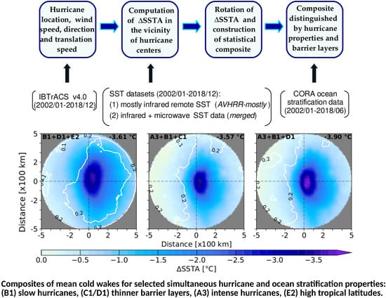
The data used and the methods applied in this study to perform the cold wake composites at observed hurricane centers are summarized in the flow chart of Figure 1. In this section, we first introduce the North Atlantic hurricane tracks and their main properties as well as the process followed to select hurricane observations (Section 2.1) that we use to construct the composites. The two SST datasets that we employ, and the methodology applied to estimate the SST anomalies (SSTA) and the hurricane-induced cooling (SSTA) are described in Section 2.2. The construction of the mean composite of SSTA (hurricane cold wake) found for the selected hurricane observations under a common reference frame and hurricane properties is presented in Section 2.3. Finally, as the cold wake is also distinguished by the upper ocean stratification, observations and methods used to compute the hurricane-induced cooling under two barrier layer metrics are described in Section 2.4.
2.1. Selection of Hurricane Observations
Hurricane tracks used in this analysis are obtained from the international best track archive for climate stewardship (IBTrACS) version 4.0, produced by the NOAA. Data is publicly available at: https://www.ncdc.noaa.gov/ibtracs/index.php?name=ib-v4-access. It combines storm data from multiple national meteorological agencies and sources to deliver the most accurate TC track data [35] and contains several variables including six-hourly information on the location of the storm center, maximum sustained wind speed at an altitude of 10 m, nature of storm origin (e.g., tropical/subtropical/extratropical), TC speed and direction.
To prepare this data for further analysis, several steps have been taken. First, only hurricanes developed in the Tropical North Atlantic Ocean were selected, including those within the Caribbean Sea and in the Gulf of Mexico. Second, 1-min maximum sustained wind speeds were converted to 10-min maximum sustained wind speeds. The IBTrACS technical guide suggests that a maximum 1-min sustained wind speed is about 12% higher than a maximum 10-min sustained wind speed [35]. The definition of a hurricane used by the National Hurricane Center (USA) is of a TC with a 10-min maximum sustained wind speed of at least 28.95 (104 ). According to the adapted 10-min maximum sustained wind speed Saffir-Simpson scale [36], TC observations over the above minimum threshold (i.e., hurricanes) were grouped in categories 1 to 5. Later, only those observations with a maximum sustained wind speed within the above definitions of category 1 and higher were considered in this study. Finally, hurricane translational speeds were computed from the locations of storm centers using 2nd order centered differences. This was done by considering the distance between the positions of the hurricane one time step before and one time step after to the passage of the hurricane, except at the first (last) time step at which a forward (backward) approach was applied respectively. After the above described steps, the number of remaining hurricane observations included in this study between years 2002 and 2018 is 1810, representing a total of 123 hurricanes.
Paths of North Atlantic hurricanes distinguished by their category are depicted in Figure 2a, while the statistical distribution of hurricanes according to their translation speed and direction (in percentage) are shown in Figure 2b–f, also divided by category. Overall, hurricanes tend to follow the large-scale low-level tropospheric anticyclonic circulation, with an initially dominant north-westward direction from the tropical to the subtropical North Atlantic to later turn north-eastward as they approach the US coast (e.g., [37]). We note that the percentage of hurricane observations that follow the westward (W), west-north-westward (WNW) and north-westward (NW) directions increases with the hurricane category, from 25% for category 1 to about 95% for category 5 observations (Figure 2b–f). It agrees with the fact that hurricanes tend to reach their maximum strength before arriving at N, from where they usually move north-eastward (Figure 2a). Moreover, in agreement with findings from Mei et al. [38], we also see that in tropical regions, where hurricanes go preferably north-westward, the most intense hurricanes (categories 3–5) tend to move faster than weaker hurricanes (categories 1–2) (Figure 2b–f).
2.2. Computation of SST Anomalies and Hurricane-Induced Cooling (SSTA)
To construct the composites of the cold wake two sets of gridded SST data (mainly) derived from satellite-based observations are employed in this study. The first dataset is the infrared optimally interpolated SST, which combines measurements from infrared remote sensors with available in situ platforms. It is less suitable for cloudy regions but spans a long period (∼35 years). The second dataset is the microwave-infrared optimally interpolated SST, based on the SST measured by several remote sensors (also including some working in the microwave spectrum). It is expected that this dataset provides more reliable measurements in cloudy areas (i.e., within bands of clouds of hurricanes). As a drawback, this data covers a shorter period (∼17 years). To better isolate the effect of hurricanes on the SST first the SST anomalies (SSTA) are computed, later the procedure followed to estimate the SSTA differences between during the storm and pre-storm conditions (SSTA) will be described.
2.2.1. Mostly Infrared Optimally Interpolated SST
Among the available group for high-resolution sea surface temperature (GHRSST) SST datasets we use in this work the NOAA optimum interpolation 1/4 degree daily sea surface temperature (OISST) Analysis from the National Centers for Environmental Information (NCEI), also available at the Physical Oceanography Distributed Active Archive Center (PODAAC) as the GHRSST Level 4 AVHRR_OI Global Blended SST analysis (GDS version 2). This dataset contains daily SST gridded data with a spatial resolution of since September 1981. Gridded SST fields have been produced by optimally interpolating and extrapolating observations from the advanced very high-resolution radiometer (AVHRR) sensors carried on a set of NOAA satellites (NOAA 7/9/14/16/17/19). As we are interested in capturing the SST perturbations induced by hurricanes, this dataset has the advantage that includes information from in situ platforms such as ships and buoys. Additionally, it is largely based on the Reynolds SST dataset used in previous works [31] and is further described by [39]. The uncertainty of the analyzed SST fields yielded by this product for the tropical North Atlantic is on average of around °C during the hurricane season (June to November) for the period of study (2002–2018), and presents a small inter-annual variability (∼±0.03 °C). This dataset can be downloaded at https://podaac.jpl.nasa.gov/dataset/AVHRR_OI-NCEI-L4-GLOB-v2.0. As this dataset mostly contains infrared remote sensed data from the AVHRR sensors, for the sake of simplicity hereinafter will be labelled as AVHRR-mostly.
2.2.2. Microwave-Infrared Optimally Interpolated SST
Among the products that provide SST from blended infrared and microwave remote sense measurements, we use the GHRSST Level 4 MW_IR_OI Global Foundation Sea Surface Temperature analysis version 5.0 that been developed by Remote Sensing Systems (REMSS). This gridded product provides daily SST images since June 2002 and has been constructed through the optimal interpolation of microwave (TMI, AMSR-E, AMSR-2, WindSat, GMI) and infrared (MODIS-Terra, MODIS-Aqua, VIIRS-NPP) satellite-based data at of spatial resolution. The main advantage of this product with respect to the AVHRR-mostly is that microwave sensors offer the through-cloud capability. Despite this improvement, we note that microwave sensors have a limited performance over precipitating clouds, which usually develop within hurricanes. Moreover, one strength of this product is its relatively long time coverage and that combines information from many sensors, although the provided SST is slightly noisier, e.g., when compared to the above presented AVHRR-mostly product. The estimated uncertainty of the analyzed SST fields accompanying this product for the tropical North Atlantic is on average of around °C during the hurricane season (June to November) and for the period of study (2002–2018), increasing up to °C near the coast. Moreover, this uncertainty presents a small inter-annual variability (∼±0.05 °C). Data is available at: https://podaac-w10n.jpl.nasa.gov/w10n/allData/ghrsst/data/GDS2/L4/GLOB/REMSS/mw_ir_OI/v5.0/. Hereinafter this product will be referred simply to as the merged SST dataset, as it includes both infrared and microwave observations.
A map of the mean tropical and subtropical North Atlantic SST during the hurricane season (June to November) for the period 2002 to 2018 from the AVHRR-mostly (Figure 3a) and from the merged data (Figure 3b) indicates that a large part of the tropical Atlantic shows mean temperatures above °C. Moreover, on average there appears to be little difference between the two datasets except between the Yucatan Channel and the Greater Antilles, and in the western African coast. A more thorough assessment of the differences of both datasets in terms of the cold wake is provided in Section 3.
2.2.3. Computation of SST Anomalies (SSTA)
To isolate hurricane-induced SST changes in the tropical North Atlantic, the trend and the seasonality were first removed from all SST time series at each grid point. To subtract the linear trend a linear fit was applied. To remove seasonality, the corresponding climatological monthly mean SST from 2002 to 2018 was also subtracted to every grid point. The resulting daily SST anomalies (SSTA, centered at midday) were linearly interpolated at each grid point to match the 6-hourly temporal resolution of the hurricane track.
The probability density function of finding the minimum SSTA at a particular day with respect to hurricane passage is shown in Figure 3c. The SSTA is taken to be the mean SSTA within a radius of 100 km of a hurricane center to increase the signal-to-noise ratio. The SSTA is most likely to be minimum one day after the passage of the hurricane, which agrees with findings from Mei and Pasquero [34]. This probability is five times smaller four days after the passage of the hurricane.
2.2.4. Hurricane-Induced Cooling (SSTA)
Based in Figure 3c and after considering several combinations of SSTA differences before and after the passage of hurricanes, we have applied the following method for the estimation of hurricane-induced cooling: First, for all SST grid points within a circle of 500 km of each hurricane center, the mean SSTA between days and is computed (in which t is the day of hurricane passage) to represent the pre-storm undisturbed state; second, also for each hurricane observation, the SSTA field for the day with minimum mean SSTA within a circle of 100 km around the hurricane center between days and is retrieved (according to Figure 3c, these days show the largest probability of finding the minimum SSTA). Hurricane-induced cooling (i.e., the cold wake), named , is defined as the difference between the second and first steps. refer to the fact that SSTA is a field (a map) with a set of positions within a circle of 500 km of radius centered at each hurricane observation. It is hypothesized that includes the direct and indirect contribution to SST cooling by a given hurricane: Either by the entrainment of sub-surface cold waters due to the near-resonant process, surface turbulent mixing, advection or any other process. As the influence of surrounding tropical storms on the SSTA field before the arrival of the hurricane may exist, those observations with other storms present in the previous 10 days within a radius of 500 km have been identified and discarded. In total less than 15 cases were found.
2.3. Construction of the Composites of SSTA (Cold Wake)
Due to the diversity of hurricane directions, especially for those of categories 1–3 (Figure 2b–d), cold wakes are expected to be at a different location for every hurricane observation. Hence, the direct average of all collocated SSTA fields would substantially smooth the cold wake asymmetry in both magnitude and location. To eliminate this problem, SSTA fields are rotated depending on the direction of travel of each hurricane observation to align them all (for the sake of clarity we have chosen the northward direction, but any other choice should provide identical results). By doing this, the resulting SSTA fields from different hurricanes can be analyzed statistically without significant loss of information. To calculate the hurricane direction at a given time step the longitudinal and latitudinal coordinates are converted to Cartesian coordinates using an equirectangular projection. Subsequently, the angle of rotation is calculated using centered differences in time, except for the first (last) time steps for which a forward (backward) scheme is applied. An example showing the original and the rotated SSTA field is shown in Figure 3 in which the SSTA field under a hurricane moving toward the W (Figure 3d) has been shifted to the N (Figure 3e). This process is repeated for all hurricane observations. We note that as the SSTA grid points are defined in a geographic coordinate system, the number of acquired points per SSTA field can vary, especially with latitude. Therefore all SSTA fields have been interpolated using a bi-linear interpolation onto a synthetic mesh of of spatial resolution and 500 km of radius. Thus, the spatial structure of cooling can be evaluated statistically by considering individual or several hurricane properties such as hurricane intensity or translation speed. Uncertainties in the composites are estimated by computing the margin of error at 95% of confidence interval with a double-tailed t-Student distribution. A similar approach was applied by Lloyd and Vecchi [33], Toomey et al. [40] to estimate the composite uncertainty.
2.4. Including the Upper Ocean Stratification in the Cold Wake Composites
In addition to the hurricane intensity and translation speed, also the cold wake composites will be distinguished by the upper ocean stratification. It is hypothesized that the effect of this stratification is represented by the magnitude and spatial distribution of barrier layers. Two barrier layer metrics derived from gridded observations are used: The barrier layer thickness (BLT) and the barrier layer potential energy (BLPE). The latter is thought to better account for the salinity effects. More details on methods and data used to compute these barrier layers metrics are described below.
2.4.1. Computation of Barrier Layer Thickness (BLT) & Barrier Layer Potential Energy (BLPE)
One critical factor that modulates the entrainment of sub-surface cold water into the mixed layer is the vertical structure of the upper ocean, more specifically the relative and absolute position of the Isopycnal Layer Depth (IPLD, or mixed layer depth) and of the Isothermal Layer Depth (ITLD). The existence of a deeper ITLD together with the simultaneous presence of a fresher near-surface layer can result in the creation of a barrier layer. A variable used to characterize a barrier layer is the barrier layer thickness (BLT). Recently, the use of the barrier layer potential energy (BLPE) rather than the BLT has been proposed by Chi et al. [41]. They argued that BLPE is a more accurate representation of the variations in stratification within the ITLD. Strong SST cooling is expected for shallow IPLD and ITLD (minimal BLT and BLPE), while large values of BLT and BLPE will tend to suppress the cooling response to hurricanes by isolating cold waters located below the thermocline hence supporting the hurricane maintenance or strengthening. We will compare both metrics in this study.
BLT is defined as in [42]:
And BLPE is defined as in [41]:
where is the mean density within the ITLD, is the available potential energy when the density is homogeneous between ITLD and the surface (fully mixed water column) and is the available potential energy for the given density profile.
Isopycnal and the isothermal layer depths (IPLD and ITLD respectively) have been computed by using the density threshold method [43], as in Steffen and Bourassa [44]. Hence, given the potential density at 10 m we look for the depth (z) at which the potential density () increases 0.1 , i.e., . Then, . The ITLD is estimated as the depth at which the temperature drops °C with respect to the temperature at a depth of 10 m, . The procedure is illustrated for two locations within the tropical North Atlantic ([W, N] and [W, N], see Figure 4a,b). These panels show the original vertical profiles of temperature, salinity and the computed potential density in the upper 500 m (denoted by red, blue and black solid lines). Using the above explained threshold methods ITLD and IPLD are estimated (depicted by green and gray horizontal lines respectively). Knowing these depths and the potential density, the BLT and BLPE are computed using Equations (1) and (2) (see values located on the center-left in Figure 4a,b).
2.4.2. Ocean Stratification Data
To compute BLT and BLPE we have used the CORA (Coriolis Ocean Dataset for Reanalysis) dataset [45], which integrates in situ temperature and salinity measurements from millions of profiles by high frequency profilers (from e.g., Argo floats) and surface and sub-surface time series (from e.g., thermosalinographs and surface drifters). Optimally interpolated monthly gridded fields from January 2002 to June 2018 are available in its version 5.2 with a horizontal spatial resolution of and a vertical resolution of 5 m within the first 100 m and of 10 m at greater depths. This product has been validated through an individualized check of every included profile. It is distributed by the Copernicus Marine and Environment Monitoring Service online catalogue: http://marine.copernicus.eu/services-portfolio/access-to-products/. Potential density fields are estimated from the temperature and salinity CORA fields by using the Fofonoff and Millard [46] expressions.
The distribution of mean BLT and BLPE during the hurricane season from 2002 to 2017, based on the above CORA data, illustrates the importance of river run-off in setting the mixed layer vertical structure in the tropical North Atlantic (Figure 4c, contours for BLT and shading for BLPE). Two tongues of large BLT and BLPE are visible: One around N that extends from the mouth of the Amazon River to the central Atlantic Ocean; another that extends from the northeast of Brazil (Orinoco River) to the eastern Caribbean Islands, covering a large part of the Caribbean Sea. In both cases values of m and are found. We note that as indicated by Steffen and Bourassa [44], values of BLT and BLPE may change prior to and after the passage of hurricanes. However, it is hypothesized that the spatial heterogeneity will maintain in the tropical Atlantic Ocean since the main forcing, the river outflow, takes place all year round. Therefore, we assume that monthly values are representative of the magnitude of barrier layers.
The derived barrier layers are employed in Section 4 and Section 5 to analyze the influence of the upper ocean stratification on the magnitude, spatial structure and temporal evolution of the cold wake. To this end, a comparison of the composites of SSTA obtained from the SST data for a set of BLT and BLPE intervals will be analyzed individually as well as in combination with the above hurricane properties (hurricane intensity and translation speed). For each observation, the closest in time monthly BLT/BLPE field was assigned. A representative value of BLT/BLPE was calculated by applying inverse distance weighting to the four BLT/BLPE grid points around the location of each hurricane center. For those hurricane observations during the months in which CORA data is not available (July to November 2018), the corresponding monthly climatological median value of CORA fields from 2002 to 2017 has been used. The reason for this is that the median value minimizes the effect of a large inter-annual spread. To conclude this section, we remark that most of the near the coast points, in which the estimated uncertainty for the merged SST product is slightly larger, will not be included in the results presented in Section 4, Section 5 and Section 6 since in these regions there are also missing or wrong (negative) values of BLT and BLPE.
3. Differences in the Cold Wake Obtained from Mostly Infrared and Infrared + Microwave SST Data
Despite the good spatial resolution and excellent temporal coverage of infrared satellite-based data, Hart et al. [28] and Dare and McBride [32] pointed out the likely underestimation of SST cooling by the AVHRR sensor under TC conditions due to its inability to retrieve a valid value of SST in cloudy environments. To partly overcome this limitation, Mei and Pasquero [34] used microwave-based SST data, more suitable to characterize cold wakes because of its through-cloud capability. However, we note again that microwave sensors are also inaccurate under precipitating clouds, which usually develop within a hurricane. To our knowledge, no study has quantified this potential underestimation in terms of the cold wake. In this section, we use the composite method described in Section 2.3 to quantify the difference in the shape and amplitude of cold wakes between AVHRR-mostly and merged SST data under TC observations from 2002 to 2018. In our discussion we hypothesize that as suggested by previous works and the already explained technical issues, the information provided by the merged dataset is, although inaccurate, closer to the truth than the AVHRR-mostly.
Panels showing the mean composite of SSTA for AVHRR-mostly and merged SST data, as well as the difference between both composites for all hurricane observations are shown in Figure 5a,c (numbers are summarized in Table 1 with uncertainties at 95% of confidence). The minimum values of SSTA (referred to as ) are °C and °C for AVHRR-mostly and merged respectively, with an average underestimation of around °C for AVHRR-mostly SST. A smaller difference is found when we compute the average SSTA over a disk of 200 km of radius around the hurricane center (), with values of −0.97 °C and −1.19 °C for AVHRR-mostly and merged SST respectively. The spatial distribution of SSTA shows that the main differences between AVHRR-mostly and merged SST are located around the center-right region (Figure 5c,f,i,l).
A further assessment of the SSTA is performed by splitting the hurricane observations into three groups according to their category: 1, 2 and 3–5 (major hurricanes). Results indicate that the underestimation of the magnitude of by AVHRR-mostly is larger for the strongest hurricanes (category 2 and higher, Figure 5d–l) with values over °C than for the hurricanes of category 1 (°C), without taking into account SST datasets uncertainties. This is likely explained by the presence of more developed (thicker) vertical clouds under stronger hurricanes. Overall category 2 hurricanes show a slightly more intense cooling than categories 3–5 hurricanes (below °C for merged SST), but with both values included within the margin of error (Table 1).
More information on the spatial structure of the cold wake is provided by a left-right cross-section of SSTA along the x-axis at (Figure 5m,n). It shows a similar position of the maximum cooling () (on the right and near the center) for both data. Indeed the is a bit closer to the center for merged SST (60 and 50 km for AVHRR-mostly and merged data respectively if all hurricanes are considered). This difference may be partly due to the coarser spatial resolution of AVHRR-mostly product. Slightly larger differences are found for the cold wake width, with a relative overestimation of around 30 km for AVHRR-mostly data (510 and 480 km respectively). One interesting result is that the cold wake width (as estimated) decreases clearly with the hurricane strength in merged SST (from 530 to 420 km), while this decrease is smaller for AVHRR-mostly SST (from 520 to 490 km). The width has been computed as the separation between the e-folding decay of around the position of : i.e., , where and , where the + and − signs of indicate that they are located on the right and on the left of respectively. Therefore, a shorter width is related to a more abrupt decay in space of (i.e., a larger temperature gradient).
Our results evidence that the use of SST data with information from microwave sensors is critical to accurately capture the SST under atmospheric structures such as hurricanes, which have very thick clouds and large rain bands. Therefore, in the following sections only the merged SST will be considered.
4. Cold Wake Composites for Selected Hurricane and Oceanic Properties
In this section, we evaluate the composites of SSTA conditioned to a set of hurricane and oceanic mixed layer properties. First, the assessment is performed for the following individual characteristics: Hurricanes intensity and translational speed, barrier layer thickness (BLT) and barrier layer potential energy (BLPE). Next, a combined analysis of SST cooling considering the synergistic effect of two (or more) parameters is discussed.
4.1. Cold Wake Composites for Individual Properties
The probability density functions (PDF) for the selected observations of hurricane 10-min maximum sustained wind speed and translation speed, the barrier layer thickness (BLT) and the barrier layer potential energy (BLPE) are shown in Figure 6. For further analysis, observations have been divided into three groups according to their percentile within the corresponding PDF distributions. Thresholds separating these three groups are denoted by vertical dashed lines (percentiles 33 and 67 are referred to as P33 and P67). The median of these distributions are for 10-min maximum sustained wind speed (Figure 6a), for translational speed (Figure 6b), for BLT (Figure 6c) and for BLPE (Figure 6d). We note that the secondary peak in the wind speed for values has been found in previous studies, and is associated with the rapid intensification of major hurricanes [47]. The mean composites of of these individual properties and for three percentile ranges are shown in Figure 7, and a detailed summary is available in Table 2. A further discussion for each property is presented below.
We find for stronger winds a stronger cooling (for max. sustained wind speed below P33 the mean minimum cooling is °C, while for observations with winds over P67 cooling is °C, Figure 7(A1–A3). However, cooling difference between ≤P33 and between P33 and P67 (Figure 7(A1,A2)) is larger than between P33-P67 and >P67 (Figure 7(A2,A3)), which is on average rather small (<0.1 °C, Table 2).
In terms of the translation speed (Figure 7(B1–B3)), slower hurricanes tend to generate a colder wake. This cooling weakens significantly for faster hurricanes. Differences between B1–B3 are much larger than the margin of error at of confidence. On average up to 50% less cooling is found for fast-moving hurricanes compared to slow-moving hurricanes (°C and °C respectively), which is in agreement with the ratio found by Mei and Pasquero [34].
The vertical structure of the upper ocean also affects the magnitude and spatial signature of cooling. As shown in Figure 4c, large values of BLT and BLPE are found in regions where significant river plumes are present, presumably due to the input of fresh waters in the upper layers that aid to create a stratified sub-layer within the mixed layer. Composites of SSTA are also grouped into three percentile intervals of BLT and BLPE. We find more cooling for the smallest BLT and BLPE percentile range (≤P33, Figure 7(C1,D1) and Table 2), with an average mean strongest cooling of °C and °C respectively. When BLPE and BLT are smaller, stronger cooling is found for BLPE than for BLT. For larger values of BLT and BLPE cooling is progressively reduced to an average value of °C and °C respectively, which represents a decrease of around 32% and 43% (Figure 7(C3,D3)). In case of moderate values of BLT and BLPE the resulting mean maximum cooling is almost the same, about °C (Figure 7(C2,D2)).
Based on the above results, the cross-section in the perpendicular direction with respect to the hurricane movement of the mean SSTA at for those individual cases of each property that yield the strongest cooling (A3, B1, C1 and D1) are shown in Figure 8a. In all cases, is located on the right but close to the center (at around 50 km) thus reflecting the known cold wake asymmetry (e.g., [34]). The magnitude of cooling decreases when the average of SSTA is taken over a disk of 200 km around the hurricane center. It is inferred from Figure 8 that the largest deviation is localized around the region of strongest cooling, in the eyewall, which hosts the maximum updraft within hurricanes [48]. Interestingly, the position of () moves to the right as the hurricane translation speed increases ( increases from 40 km for slower hurricanes to 80 km for faster hurricanes, Table 2).
When the mean strongest cooling () found according to the above analyzed individual parameters is ordered from greater to smaller cooling, the most relevant factor is the hurricane translational velocity, followed by the ocean mixed layer structure (BLPE and BLT) and the hurricane category, which appears to play a relatively less important role.
4.2. Cold Wake Composites for Combined Properties
Next we investigate to what extent the cold wake is modified when two or three of the above analyzed properties are considered simultaneously. Among all possible combinations of two and three of those properties shown in Table 2, only those cases yielding the strongest cooling are summarized in Table 3.
Our results indicate that the combinations of two properties with the strongest cooling are those in which a slow-moving hurricane passes over a region with a small BLT (case B1+C1) or BLPE (case B1+D1). These two cases tend to induce more cooling than a slow-moving hurricane with very intense maximum sustained winds (B1+A3) with of about °C, °C and °C respectively (Figure 8b, Figure 9 top row, and Table 3). As for the individual cases with slow-moving hurricanes (compare B1–B3, Table 2), the perpendicular cross-sections also indicate that shifts to the center ( km) thus reducing the rightward asymmetry. The cold wake width is slightly larger (∼40 km) for the combined B1+D1 case, as can be appreciated in Figure 9 and in Figure 8b (red line). An interesting point to mention is that for thin barrier layers the BLPE presents more sensitivity to capture the hurricane-induced cooling (with average values of about °C lower than for the BLT parameter), while for thicker barrier layers BLPE shows less cooling (Table 2). This suggests that BLPE is more suitable to capture barrier layer nuances, and hence to better reproduce hurricane-induced cooling.
As with the above-discussed combinations of two properties, we look for the synergistic effect of three of the analyzed properties that yield the strongest cooling. Among all possibilities two combinations excel: First, the case A3+B1+D1 with around °C; Second, the case A3+B1+C1 with of °C (Figure 9 bottom row and Table 3). Thus, the strongest cooling is obtained when simultaneously hurricanes are very intense, move slow and pass over an oceanic region with low BLT/BLPE.
Previous studies have pointed out the relevance of the latitudinal position of hurricane observations in the amplitude of the cold wake (e.g., [34]). To investigate this, we have grouped hurricanes in three ranges: (E1) N, (E2) 20–30N and (E3) N. As expected, the strongest cooling is found for the E2 case. This is the region where most hurricanes reach their major strength (see red color in Figure 2a). When the latitude of hurricane observations is simultaneously analyzed together with the other properties, the strongest cooling is found for the combination B1+D1+E2 (with a value of °C). We note that this cooling is smaller than the °C previously found for the case A3+B1+D1 and similar to the case A3+B1+C1 (Figure 9, bottom row). Therefore, these results indicate that in terms of cooling, the hurricane strength appears to be a more relevant property.
Interestingly, when we consider the spatial average of cooling (), the inclusion of the latitude yields more mean cooling than the hurricane strength, with values of °C and °C respectively. However, note that due to the smaller number of observations, the margin of error is larger when three parameters are considered, reaching even values near °C for and of °C for . Therefore, the three cases with strongest cooling (A3+B1+D1, A3+B1+C1 and B1+D1+E2) fall inside the range of uncertainties and are statistically hardly distinguishable.
5. Temporal Evolution of the Cold Wake for Selected Hurricane and Oceanic Properties
An important characteristic associated with the cold wake is how its spatial structure and magnitude change with time. In particular: How much time does it take for the cold wake to disappear? How does this time change with the individual hurricane and ocean properties evaluated in Section 4?
To address these questions, we have analyzed the temporal evolution of and as follows: First, for every hurricane observation time series of and have been constructed starting at the day of (which as explained in Section 2, can occur between and days for each hurricane observation); second, these time series have been daily averaged and grouped considering those study cases described in Table 2; Finally, as in Mei and Pasquero [34], the resulting daily time series have been fitted against an exponential function: , in which A is the value of and at , t is the time after and is the rate of decay (unit of in both cases). In this way, the fitting expressions can be simply rewritten as: and .
The average values of the scaled with respect to the number of days after as well as the fitting curve are shown in Figure 10 (distinguished by properties studied in Section 4 and percentile ranges shown in Table 2).
Overall, rates of decay () are rather similar for all study cases with values between 9.1 and 11.7 (B3 and B2 respectively). The fastest decay of the cold wake is found for the B3, D3 and B1 cases, while the slowest decay is shown by the D2, A2 and B2 cases. Interestingly, shows small differences between cases C1–C3 (BLT), pointing out that the state of the upper ocean stratification before and during the passage of the hurricane has a small effect on the rate of restratification of the water column once the hurricane has left the region.
More in detail, during the first 15–20 days after the passage of the hurricane the largest cooling decreases in magnitude rather fast, decaying exponentially 80% with respect to the initial value for all study cases (see the decay from 1 to 0.2 at y-axis around 15 days after the minimum SSTA in Figure 10). After 20 days, the behavior is more complex as it depicts some oscillations over a weaker decreasing trend, taking around 30 to 40 more days to reach the original SSTA conditions previous to the arrival of the hurricane.
For a similar exponential decay is found (not shown), except that the time needed to recover the initial condition is about 10 days longer (for a total of around 60 days). This is likely explained by the fact that in this case the temperature of a large area (a circle of 200 km of radius) has to become homogeneous, which is expected to take on average more time than a single point. Moreover, fluctuations are larger, as reflected in the range of (with values between 10.5 and 15.1 ).
Based on our results, the answers to the questions formulated in the beginning of this section are: (1) how much time does it take for the cold wake to disappear? On average the strong cold anomalies induced by a hurricane need around 50–60 days to (almost) disappear and recover the climatological mean values; (2) How does this time change with the individual hurricane and ocean properties evaluated in Section 4? We have not found any evidence that the evolution of the cold wake is affected by the hurricane properties and the ocean mixed layer vertical structure. This suggests little memory in the cold wake restratification process and a high dependence on the environmental conditions, in good agreement with Mei and Pasquero [34].
To conclude this section, we note that a better comprehension of the temporal evolution of the cold wake could be potentially provided by a detailed study of the upper ocean heat content. However, current long-term gridded products (mostly derived by blending satellite-derived SST and in situ profilers) present some problems in resolving the hurricane-induced ocean heat content perturbation at daily scales. The reason is that in the absence of nearby in situ mixed layer data climatologies are used instead.
6. Insights on Hurricane Intensity Response to Cold Wake
Although the main aim of this work is to assess the cold wake amplitude and structure, in this section we briefly investigate if any connection exists between the observed SST cooling and the hurricane maximum sustained surface wind speed () provided by IBTrACS data. We note that in principle, observations used in this work do not allow explanation of whether hurricane intensification/weakening is causally related with the magnitude of absolute SST or cold wake properties. Previous studies have found that the SST cooling is usually accompanied by a weakening of TCs (e.g., [18,49,50,51]). The magnitude of this weakening is larger for those hurricanes moving slower and where the largest SST cooling is located [17,18]. For instance, Schade and Emanuel [52] systematically analyzed the atmospheric response to SST (the evaporation-wind feedback process so-called SST feedback effect or WISHE mechanism) using a coupled model in which also the sensitivity to several other parameters was evaluated (e.g., storm translation speed and size, relative humidity, momentum and heat transfer coefficients or tropopause temperature), pointing out the major relevance of SST in controlling the TC intensity, with a potential storm weakening of up to 50% due to SST feedback reflected in the reduction of enthalpy fluxes caused by the SST cooling. Alternatively to the mentioned WISHE mechanism, other model-based studies found that the SST has a minor relevance in the intensification of TCs once a certain SST threshold has been attained, and that non-linear local atmospheric processes in the boundary layer may lead to a stronger TC mean flow (e.g., [53,54,55]).
To investigate the possible influence of the cold wake on the hurricane strength, we have divided the change in the wind speed for each hurricane observation in the first 24 h () into four groups (see also Table 4, unit in kt/24 h, where 1 kt ≈ 0.51, m·s): Weakening (WK) for , neutral response (NR) for , slow intensification (SI) for and rapid intensification (RI) for . For all hurricane observations within each group the mean and the margin of error at 95% of confidence have been computed. In addition to , other variables have been included in the assessment such as: The mean SST (), the largest cooling (), BLT, BLPE, the mean latitude of the hurricane () and the hurricane translation speed ().
Table 4 indicates that in most cases, remains neutral or weakens (∼1150 of about 1500 observations). On average, it occurs more often at higher latitudes (N), over lower SST (°C) and for strong cooling (°C). This response is in line with results of modeling studies (e.g., [18,56,57]) and the WISHE mechanism.
The reminding observations (around 25%) show slow or rapid intensification (SI and RI), which occur when the mean SST is larger and when the cooling is smaller. In more detail, RI is found for °C and °C. Hurricane intensification seems to be associated with originally weaker hurricanes (, i.e., hurricanes with theoretical margin to develop more), and with hurricanes located in lower latitudes (N) that are likely characterized by warmer waters (Figure 2). Besides, as they feel a positive SST gradient, likely stronger momentum and enthalpy fluxes may develop [51,52].
In contrast, no clear differences are found in terms of the hurricane translation speed () between NR, SI and RI cases. However, weakened hurricanes tend on average to move slightly faster ( more). Similarly, the role of initial conditions of BLT and BLPE on hurricane intensification is unclear as they present a very large spatial variability (see the large margin of error), although it is expected that their effect in momentum and enthalpy fluxes is already being indirectly reflected in .
As noted above, hurricane intensification can also be triggered by atmospheric-driven processes if SST is over 27–28 °C (e.g., [53,55]). This intensification can occur when the hurricane moves to a region in which atmospheric conditions are more favorable (e.g., higher boundary layer air temperature, favorable environmental vorticity, or more reduced vertical wind shear). Indeed, the simultaneous occurrence of favorable oceanic and atmospheric conditions is also possible. Based on the high complexity of these processes the combination of simultaneous air-sea measurements and coupled high-resolution simulations is necessary to fully understand the atmospheric feedback to SST cooling, which is far beyond the scope of this work.
7. Conclusions
This study had two main objectives: First, try to reconcile the large dispersion of values of observed hurricane-induced SST cooling yielded by previous works in the North Atlantic Ocean, which were based on individual or a large ensemble of hurricanes and used infrared- and/or microwave-based remote observations; and second, to quantify the sensitivity of SST cooling under a set of hurricane and oceanic parameters: Hurricane 10-min maximum sustained wind speed, hurricane translation speed, and the ocean mixed layer structure by means of the barrier layer thickness and the barrier layer potential energy (BLT and BLPE). To this end, a statistical composition of a large amount of hurricane observations under the same reference system has been performed.
We have found that the spatial structure of the cold wake (position of largest cooling and cold wake width) does not show clear differences when infrared (AVHRR-mostly) or when infrared+microwave SST data (merged) is used (Table 1). However, in terms of the amplitude of the cold wake, differences are evident, with a relative underestimation by infrared data of around 0.4–0.5 °C in the magnitude of largest cooling (Table 1 and Figure 5).
Ordered from larger to lower magnitude of cooling, the translation speed is the most important property once the tropical storm has reached hurricane category. It has a critical role in the position of strongest cooling with respect to the hurricane center ( in Table 2), which approaches the center as the hurricane translation speed decreases confirming results by Mei and Pasquero [34]. This rightward bias is 80 km for the one third fastest moving hurricanes and 40 km for the one third slowest moving hurricanes, with a mean position of around 60 km to the right of the center of the hurricane, very close to the radius of maximum sustained wind, which agrees with other observed and model-based studies such as Price [14], Steffen and Bourassa [44]. Indeed Price [14], Jullien et al. [22] found an enhanced upwelling along the hurricane track for slow-moving hurricanes.
The second most important property with respect to the amount of cooling is the upper ocean vertical structure. In contrast to Mei and Pasquero [34], who used an analytic approach to estimate mixed layer depth at typical values of the tropical regions, we have used a monthly gridded climatology constructed with observations. Although Lloyd and Vecchi [33] also used observations, their dataset only took into account the stratification in temperature but not in salinity.
The mean composite of those hurricane observations passing over regions with values of BLPE within the first third of the percentile range (P33, Figure 5) yield slightly stronger cooling than for the first third of BLT (∼0.15 °C, Table 2 and Figure 7). On average, differences in the barrier layer properties can impact the magnitude of largest cooling up to 1–1.5 °C if uncertainties are considered (Table 2).
Differences in the SST cooling induced by hurricanes of different categories appears to be less important when compared to the hurricane moving speed and the upper ocean stratification. As an example, hurricanes of categories 3–5 induce almost the same cooling as hurricanes of category 2 (∼0.1 °C), which is in line with findings in the North Atlantic from Michaels et al. [24], Lloyd and Vecchi [33] and different from [34], who found a stronger cooling of about °C for TCs of categories 3–5. Although in their case they included all TCs in the Northern Hemisphere thus merging Pacific and Atlantic Ocean upper ocean conditions and responses. In this regard, Lloyd and Vecchi [33] already mentioned that this non-monotonic response of SST cooling with hurricane intensity is especially remarkable in the North Atlantic.
Overall the above results are in line with previous works, which already indicated that the average amplitude of SST cooling is larger for slow-moving hurricanes over those regions with small values of BLT/BLPE (e.g., [26,44]). We have found that for those cases in which all these conditions are met, the mean largest cooling reaches values below °C (Table 3). This magnitude of cooling, larger for BLPE than for BLT (Table 3), is of the same order of that obtained from individual observations (e.g., [8,9,23]), but is larger than statistical insights from Michaels et al. [24], Hart et al. [28] since they only used infrared SST data. Moreover, this work presents an improvement with respect to Lloyd and Vecchi [33], Mei and Pasquero [34] since our results are regionalized for the North Atlantic and include the effect of more realistic barrier layers, thus integrating the combined effect of hurricane and ocean properties.
Regarding the temporal variability of the cold wake, our results show a fast exponential decay in the magnitude of cooling (of about 80%) during the first 20 days, to later decay more slowly almost up to pre-hurricane conditions in about 50–60 days (Figure 10). This value is around 20 days longer than the one found by Hart et al. [28], a difference that could be explained by their use of infrared data. Moreover, contrary to what was suggested by Lloyd and Vecchi [33], on average we have not found a residual cooling after two months. This does not imply that it may not exist for individual cases. The time needed by the cold wake to disappear does not show a statistical dependency on the hurricane properties nor on the ocean mixed layer structure prior or during the passage of the hurricane. Therefore, the restoring time appears to be strongly dominated by the environmental conditions, as already pointed out by Mei and Pasquero [34], so the final recovery time may change from case to case.
We note that due to the lack of reliable information on the hurricane size, this parameter has not been included in our analysis. However, observations indicate that the radius of maximum wind changes little with hurricane category (with values between 40–60 km, decreasing with category) [58], thus small changes in the cold wake structure are expected.
Some indications on the mean 10-min maximum sustained wind response to the cold wake are summarized in Table 4. Most of hurricane observations (75%) show a weakening or little change in the wind intensity. The remainder of the observations shown some kind of intensification, with few observations showing a rapid intensification, mostly reserved for hurricanes below category 3, over very warm waters (>28 °C) in tropical areas (<22N). However, the high degree of complexity of the involved processes and the atmospheric feedback requires a more complete assessment to elucidate the chain of physical processes involved in the atmospheric response. To this end, the combination of simultaneous air-sea measurements and high-resolution coupled simulations will be necessary [1].
Author Contributions
Conceptualization by J.-M.S and C.A.K.; methodology developed by K.H. and J.-M.S.; formal analysis and visualization by K.H.; original draft prepared by J.-M.S. with contributions from K.H., C.G.v.d.B. and C.A.K. All authors have reviewed and approved the final version of this manuscript.
Funding
This research received no external funding.
Acknowledgments
Juan-Manuel Sayol and Caroline A. Katsman thank the financial support by the Netherlands Scientific Research foundation (NWO) through the VIDI grant number 864.13.011 awarded to Caroline A. Katsman.
Conflicts of Interest
The authors declare no conflict of interest.
References
- Emanuel, K. 100 Years of Progress in Tropical Cyclone Research. Meteorol. Monogr. 2018, 59, 15.1–15.68. [Google Scholar] [CrossRef]
- Fisher, E.L. Hurricanes and the sea-surface temperature field. J. Meteor. 1958, 15, 328–333. [Google Scholar] [CrossRef]
- Perlroth, I. Relationship of central-pressure of hurricane Esther (1961) and the sea-surface temperature field. Tellus 1962, 14, 403–408. [Google Scholar] [CrossRef]
- Leipper, D.F. Observed Ocean Conditions and Hurricane Hilda, 1964. J. Atmos. Sci. 1967, 24, 182–186. [Google Scholar] [CrossRef] [Green Version]
- Hazelworth, J.B. Water temperature variations resulting from hurricanes. J. Geophys. Res. 1968, 73, 5105–5123. [Google Scholar] [CrossRef]
- Stramma, L.; Cornillon, P.; Price, J.F. Satellite observations of sea surface cooling by hurricanes. J. Geophys. Res. 1986, 91, 5031–5035. [Google Scholar] [CrossRef]
- Jordan, C.L. On the influence of tropical cyclones on the sea surface temperature. In Proceedings of the Symposium on Tropical Meteorology; Hutchings, J.W., Ed.; New Zealand Meteorological Service: Wellington, New Zealand, 1964; pp. 614–622. [Google Scholar]
- Shay, L.K.; Black, P.G.; Mariano, A.J.; Hawkins, J.D.; Elsberry, R.L. Upper ocean response to Hurricane Gilbert. J. Geophys. Res. Oceans 1992, 97, 20227–20248. [Google Scholar] [CrossRef] [Green Version]
- Monaldo, F.M.; Sikora, T.D.; Babin, S.M.; Sterner, R.E. Satellite Imagery of Sea Surface Temperature Cooling in the Wake of Hurricane Edouard (1996). Mon. Weather Rev. 1997, 125, 2716–2721. [Google Scholar] [CrossRef]
- Wang, B.; Xiang, B.; Lee, J.Y. Subtropical high predictability establishes a promising way for monsoon and tropical storm predictions. Proc. Natl. Acad. Sci. USA 2013, 110, 2718–2722. [Google Scholar] [CrossRef]
- Sriver, R.L.; Huber, M. Modeled sensitivity of upper thermocline properties to tropical cyclone winds and possible feedbacks on the Hadley circulation. Geophys. Res. Lett. 2010, 37. [Google Scholar] [CrossRef] [Green Version]
- Huang, S.M.; Oey, L.Y. Right-side cooling and phytoplankton bloom in the wake of a tropical cyclone. J. Geophys. Res. Oceans 2015, 120, 5735–5748. [Google Scholar] [CrossRef]
- Ichiye, T. Response of a two-layer ocean with a baroclinic current to a moving storm, Part II—Non-geostrophic baroclinic mode. J. Oceanogr. Soc. Jpn. 1977, 33, 169–182. [Google Scholar] [CrossRef]
- Price, J.F. Upper Ocean Response to a Hurricane. J. Phys. Oceanogr. 1981, 11, 153–175. [Google Scholar] [CrossRef] [Green Version]
- Shay, L.K.; Goni, G.J.; Black, P.G. Effects of a Warm Oceanic Feature on Hurricane Opal. Mon. Weather Rev. 2000, 128, 1366–1383. [Google Scholar] [CrossRef]
- Mao, Q.; Chang, S.W.; Pfeffer, R.L. Influence of Large-Scale Initial Oceanic Mixed Layer Depth on Tropical Cyclones. Mon. Weather Rev. 2000, 128, 4058–4070. [Google Scholar] [CrossRef]
- Morey, S.L.; Bourassa, M.A.; Dukhovskoy, D.S.; O’Brien, J.J. Modeling studies of the upper ocean response to a tropical cyclone. Ocean Dyn. 2006, 56, 594–606. [Google Scholar] [CrossRef]
- Bender, M.A.; Ginis, I.; Kurihara, Y. Numerical simulations of tropical cyclone-ocean interaction with a high-resolution coupled model. J. Geophys. Res. Atmos. 1993, 98, 23245–23263. [Google Scholar] [CrossRef]
- Greatbatch, R.J. On the Response of the Ocean to a Moving Storm: The Nonlinear Dynamics. J. Phys. Oceanogr. 1983, 13, 357–367. [Google Scholar] [CrossRef] [Green Version]
- Zedler, S.E. Simulations of the Ocean Response to a Hurricane: Nonlinear Processes. J. Phys. Oceanogr. 2009, 39, 2618–2634. [Google Scholar] [CrossRef]
- Yablonsky, R.M.; Ginis, I. Limitation of One-Dimensional Ocean Models for Coupled Hurricane–Ocean Model Forecasts. Mon. Weather Rev. 2009, 137, 4410–4419. [Google Scholar] [CrossRef]
- Jullien, S.; Menkes, C.E.; Marchesiello, P.; Jourdain, N.C.; Lengaigne, M.; Koch-Larrouy, A.; Lefèvre, J.; Vincent, E.M.; Faure, V. Impact of Tropical Cyclones on the Heat Budget of the South Pacific Ocean. J. Phys. Oceanogr. 2012, 42, 1882–1906. [Google Scholar] [CrossRef] [Green Version]
- Cione, J.J.; Uhlhorn, E.W. Sea Surface Temperature Variability in Hurricanes: Implications with Respect to Intensity Change. Mon. Weather Rev. 2003, 131, 1783–1796. [Google Scholar] [CrossRef] [Green Version]
- Michaels, P.J.; Knappenberger, P.C.; Davis, R.E. Sea-surface temperatures and tropical cyclones in the Atlantic basin. Geophys. Res. Lett. 2006, 33. [Google Scholar] [CrossRef] [Green Version]
- Wang, X.; Han, G.; Qi, Y.; Li, W. Impact of barrier layer on typhoon-induced sea surface cooling. Dyn. Atmos. Oceans 2011, 52, 367–385. [Google Scholar] [CrossRef]
- Balaguru, K.; Chang, P.; Saravanan, R.; Leung, L.R.; Xu, Z.; Li, M.; Hsieh, J.S. Ocean barrier layers’ effect on tropical cyclone intensification. Proc. Natl. Acad. Sci. USA 2012, 109, 14343–14347. [Google Scholar] [CrossRef]
- Sprintall, J.; Tomczak, M. Evidence of the barrier layer in the surface layer of the tropics. J. Geophys. Res. Oceans 1992, 97, 7305–7316. [Google Scholar] [CrossRef] [Green Version]
- Hart, R.E.; Maue, R.N.; Watson, M.C. Estimating Local Memory of Tropical Cyclones through MPI Anomaly Evolution. Mon. Weather Rev. 2007, 135, 3990–4005. [Google Scholar] [CrossRef]
- Emanuel, K.A. An Air-Sea Interaction Theory for Tropical Cyclones. Part I: Steady-State Maintenance. J. Atmos. Sci. 1986, 43, 585–605. [Google Scholar] [CrossRef]
- Emanuel, K.A. The Maximum Intensity of Hurricanes. J. Atmos. Sci. 1988, 45, 1143–1155. [Google Scholar] [CrossRef]
- Reynolds, R.W.; Smith, T.M.; Liu, C.; Chelton, D.B.; Casey, K.S.; Schlax, M.G. Daily High Resolution Blended Analysis for sea surface temperature. J. Clim. 2007, 20, 5473–5496. [Google Scholar] [CrossRef]
- Dare, R.A.; McBride, J.L. Sea Surface Temperature Response to Tropical Cyclones. Mon. Weather Rev. 2011, 139, 3798–3808. [Google Scholar] [CrossRef]
- Lloyd, I.D.; Vecchi, G.A. Observational Evidence for Oceanic Controls on Hurricane Intensity. J. Clim. 2011, 24, 1138–1153. [Google Scholar] [CrossRef]
- Mei, W.; Pasquero, C. Spatial and Temporal Characterization of Sea Surface Temperature Response to Tropical Cyclones. J. Clim. 2013, 26, 3745–3765. [Google Scholar] [CrossRef]
- Knapp, K.R.; Kruk, M.C.; Levinson, D.H.; Diamond, H.J.; Neumann, C.J. The International Best Track Archive for Climate Stewardship (IBTrACS). Bull. Am. Meteorol. Soc. 2010, 91, 363–376. [Google Scholar] [CrossRef]
- Regional Association IV (North America, Central America and the Caribbean). Hurricane Operational Plan; Technical Document wmo-td No. 494; Tropical Cyclone Programme; Report No. tcp-30; Secretariat of the Word Meteorological Organization: Geneva, Switzerland, 2015. [Google Scholar]
- Chadee, X.T.; Clarke, R.M. Daily near-surface large-scale atmospheric circulation patterns over the wider Caribbean. Clim. Dyn. 2015, 44, 2927–2946. [Google Scholar] [CrossRef]
- Mei, W.; Pasquero, C.; Primeau, F.O. The effect of translation speed upon the intensity of tropical cyclones over the tropical ocean. Geophys. Res. Lett. 2012, 39. [Google Scholar] [CrossRef] [Green Version]
- Banzon, V.; Smith, T.M.; Chin, T.M.; Liu, C.; Hankins, W. A long-term record of blended satellite and in-situ sea-surface-temperature for climate monitoring, modeling and environmental studies. Earth Syst. Sci. Data 2016, 8, 165–176. [Google Scholar] [CrossRef]
- Toomey, T.; Sayol, J.M.; Marcos, M.; Jordà, G.; Campins, J. A modelling-based assessment of the imprint of storms on wind waves in the western Mediterranean Sea. Int. J. Climatol. 2019, 39, 878–886. [Google Scholar] [CrossRef]
- Chi, N.H.; Lien, R.C.; D’Asaro, E.A.; Ma, B.B. The surface mixed layer heat budget from mooring observations in the central Indian Ocean during Madden–Julian Oscillation events. J. Geophys. Res. Oceans 2014, 119, 4638–4652. [Google Scholar] [CrossRef]
- Foltz, G.R.; McPhaden, M.J. Impact of Barrier Layer Thickness on SST in the Central Tropical North Atlantic. J. Clim. 2009, 22, 285–299. [Google Scholar] [CrossRef]
- de Boyer Montégut, C.; Madec, G.; Fischer, A.S.; Lazar, A.; Iudicone, D. Mixed layer depth over the global ocean: An examination of profile data and a profile-based climatology. J. Geophys. Res. Oceans 2004, 109. [Google Scholar] [CrossRef]
- Steffen, J.; Bourassa, M. Barrier Layer Development Local to Tropical Cyclones based on Argo Float Observations. J. Phys. Oceanogr. 2018, 48, 1951–1968. [Google Scholar] [CrossRef]
- Szekely, T.; Gourrion, J.; Pouliquen, S.; Reverdin, G. CORA 5.0: Global in situ temperature and salinity dataset. Operational Oceanography serving Sustainable Marine Development. In Proceedings of the Eight EuroGOOS International Conference, Bergen, Norway, 3–5 October 2017; Buch, E., Fernández, V., Eparkhina, D., Gorringe, P., Nolan, G., Eds.; EuroGOOS: Brussels, Belgium, 2018; pp. 439–446. [Google Scholar]
- Fofonoff, N.P.; Millard, R.C., Jr. Algorithms for the Computation of Fundamental Properties of Seawater; UNESCO Technical Papers in Marine Sciences 44; UNESCO: Paris, France, 1983. [Google Scholar]
- Soloviev, A.V.; Lukas, R.; Donelan, M.A.; Haus, B.K.; Ginis, I. The air-sea interface and surface stress under tropical cyclones. Sci. Rep. 2014, 4, 5306. [Google Scholar] [CrossRef] [PubMed]
- Stern, D.P.; Bryan, G.H.; Aberson, S.D. Extreme Low-Level Updrafts and Wind Speeds Measured by Dropsondes in Tropical Cyclones. Mon. Weather Rev. 2016, 144, 2177–2204. [Google Scholar] [CrossRef]
- Sutyrin, G.G.; Khain, A.P. Effect of the ocean-atmosphere interaction on the intensity of a moving tropical cyclone. Atmos. Oceanic Phys. 1984, 34, 787–794. [Google Scholar] [CrossRef]
- Ginis, I.; Dikinov, D.Z.; Khain, A.P. A three dimensional model of the atmosphere and the ocean in the zone of a typhoon. Dokl. Akad. Sci. USSR 1989, 307, 333–337. [Google Scholar]
- Schade, L.R. Tropical Cyclone Intensity and Sea Surface Temperature. J. Atmos. Sci. 2000, 57, 3122–3130. [Google Scholar] [CrossRef]
- Schade, L.R.; Emanuel, K.A. The Ocean’s Effect on the Intensity of Tropical Cyclones: Results from a Simple Coupled Atmosphere–Ocean Model. J. Atmos. Sci. 1999, 56, 642–651. [Google Scholar] [CrossRef]
- Montgomery, M.T.; Sang, N.V.; Smith, R.K.; Persing, J. Do tropical cyclones intensify by WISHE? Q. J. R. Meteorol. Soc. 2009, 135, 1697–1714. [Google Scholar] [CrossRef] [Green Version]
- Jullien, S.; Marchesiello, P.; Menkes, C.E.; Lefèvre, J.; Jourdain, N.C.; Samson, G.; Lengaigne, M. Ocean feedback to tropical cyclones: Climatology and processes. Clim. Dyn. 2014, 43, 2831–2854. [Google Scholar] [CrossRef]
- Smith, R.K.; Montgomery, M.T. Toward Clarity on Understanding Tropical Cyclone Intensification. J. Atmos. Sci. 2015, 72, 3020–3031. [Google Scholar] [CrossRef]
- Bender, M.A.; Ginis, I. Real-Case Simulations of Hurricane–Ocean Interaction Using a High-Resolution Coupled Model: Effects on Hurricane Intensity. Mon. Weather Rev. 2000, 128, 917–946. [Google Scholar] [CrossRef]
- Zhu, T.; Zhang, D.L. The impact of the storm-induced SST cooling on hurricane intensity. Adv. Atmos. Sci. 2006, 23, 14–22. [Google Scholar] [CrossRef] [Green Version]
- Kimball, S.K.; Mulekar, M.S. A 15-Year Climatology of North Atlantic Tropical Cyclones. Part I: Size Parameters. J. Clim. 2004, 17, 3555–3575. [Google Scholar] [CrossRef]
Figure 1.
Flow chart summarizing data and methods of this work described in Section 2. SSTA are the SST anomalies after the linear trend and the seasonality have been removed. SSTA refers to the hurricane-induced cooling (cold wake). Years refer to the common period of all datasets used in this study (2002–2018).

Figure 2.
(a) Hurricane tracks in the North Atlantic from 2002 to 2018 (both years included). Shading indicates the hurricane category according to the Saffir-Simpson scale (see legend). (b–f) Wind-roses for the hurricane categories (1 to 5 respectively) showing the probability distribution (in %) of translation speeds and directions of hurricanes.

Figure 3.
(a) Mean Sea Surface Temperature (SST) from 2002 to 2018 (both years included) during the hurricane season in the North Atlantic (June to November) for AVHRR-mostly data. Black dashed and solid contours denote SSTs of 28 °C and 29 °C respectively. (b) Same as (a) but for merged data. (c) Probability density distribution of the day of minimum sea surface temperature anomalies for all observations from 2002 to 2018 before/during/after the passage of a hurricane. (d,e) An example of rotated SSTA anomalies under a hurricane observation: (d) original field, (e) rotated field. The rotation has been done to have a hurricane moving northward.

Figure 4.
(a,b) Example of potential density (black line), temperature (red line) and salinity (blue line) derived from the CORA dataset for two grid points in the Caribbean Sea (exact location in bold numbers). The potential density has been computed with the UNESCO formula described in Fofonoff and Millard [46]. ITLD and IPLD refer to the isothermal and isopycnic layer depths, which are used to compute the barrier layer thickness (BLT) and the Barrier Layer Potential Energy (BLPE) according to Equations (1) and (2) respectively. (c) Mean BLPE (shading) and BLT (black contours) for the hurricane season (June to November) in the North Atlantic from 2002 to 2017.

Figure 5.
First column: Composite of induced by hurricanes using AVHRR-mostly data for: (a) all hurricanes, (d) hurricanes of category 1, (g) category 2, (j) categories 3–5; Second column: Same but for merged data for: (b) all hurricanes, (e) hurricanes of category 1, (h) category 2, (k) categories 3–5; Third column: Difference between first and second columns (merged−AVHRR-mostly) for: (c) all hurricanes, (f) hurricanes of category 1, (i) category 2, (l) categories 3–5; (m,n) cross-section at the center () and in the perpendicular direction to the hurricane movement (x-axis) of the composites of for AVHRR-mostly and merged datasets respectively. N is the number of observations. Uncertainties of (margin of error) are indicated by white contours in (a–l) panels and with shading in (m,n). The minimum SSTA () is written at the top-right corner in each panel. Edges of cold wakes are indicated with triangles in (m,n) with same colors than curves (see legend). Note the different range of colors used for the third column (magnitude of differences shown by the symmetric colorbar). Detailed numbers are shown in Table 1.

Figure 6.
Probability Density Functions (PDF) for all hurricanes from 2002 to 2018 (both years included): (a) 10-min maximum sustained wind speed, (b) hurricanes translation speed, (c) associated value of barrier layer thickness (BLT) and (d) associated value of barrier layer potential energy (BLPE). P33 and P67 refer to percentile 33 and percentile 67, which are indicated by vertical dashed lines in each panel.

Figure 7.
Mean composites of SSTA based on the merged SST dataset for the following parameters: (A1–A3) 10-min maximum sustained wind, (B1–B3) hurricanes translation speed, (C1–C3) barrier layer thickness (BLT), (D1–D3) barrier layer potential energy (BLPE). First column for values below percentile 33, second column for values within the range P33 and P67, third column for values over percentile 67. Percentiles are indicated in Figure 5 and in Table 2. The margin of error of SSTA is depicted by white contours.

Figure 8.
(a) Cross-sections in the perpendicular direction with respect to the hurricane movement at of mean composites of SSTA obtained from the merged SST dataset for all selected cases: A3, B1, C1, D1 (Table 2). (b) Same as (a) but for the following selected combinations: B1+A3, B1+C1, B1+D1 and A3+B1+D1 (Table 3). Shading indicates the margin of error of SSTA.

Figure 9.
Mean composites of SSTA based on the merged SST dataset for the following combination of two (top row) and three (bottom row) parameters. Top row from left to right panels: (B1+A3), (B1+C1) and (B1+D1); Bottom row from left to right panels: (B1+D1+E2), (A3+B1+C1) and (A3+B1+D1). White contours represent the margin of error of SSTA. More information is provided in Table 3.

Figure 10.
Mean composited time series of observed obtained from the merged SST dataset after the passage of hurricanes scaled by their initial value (i.e., corresponding induced largest cooling). Observations are denoted by dots, while the exponential fittings are depicted by solid lines. Observations have been separated according to the individual parameters shown in Table 2: (a) maximum sustained wind speed cases A1–A3, (b) hurricane translation speed cases B1–B3, (c) Barrier Layer Thickness (BLT), cases C1–C3, (d) Barrier Layer Potential Energy, (BLPE) cases D1-D3 (see legends). has units of .


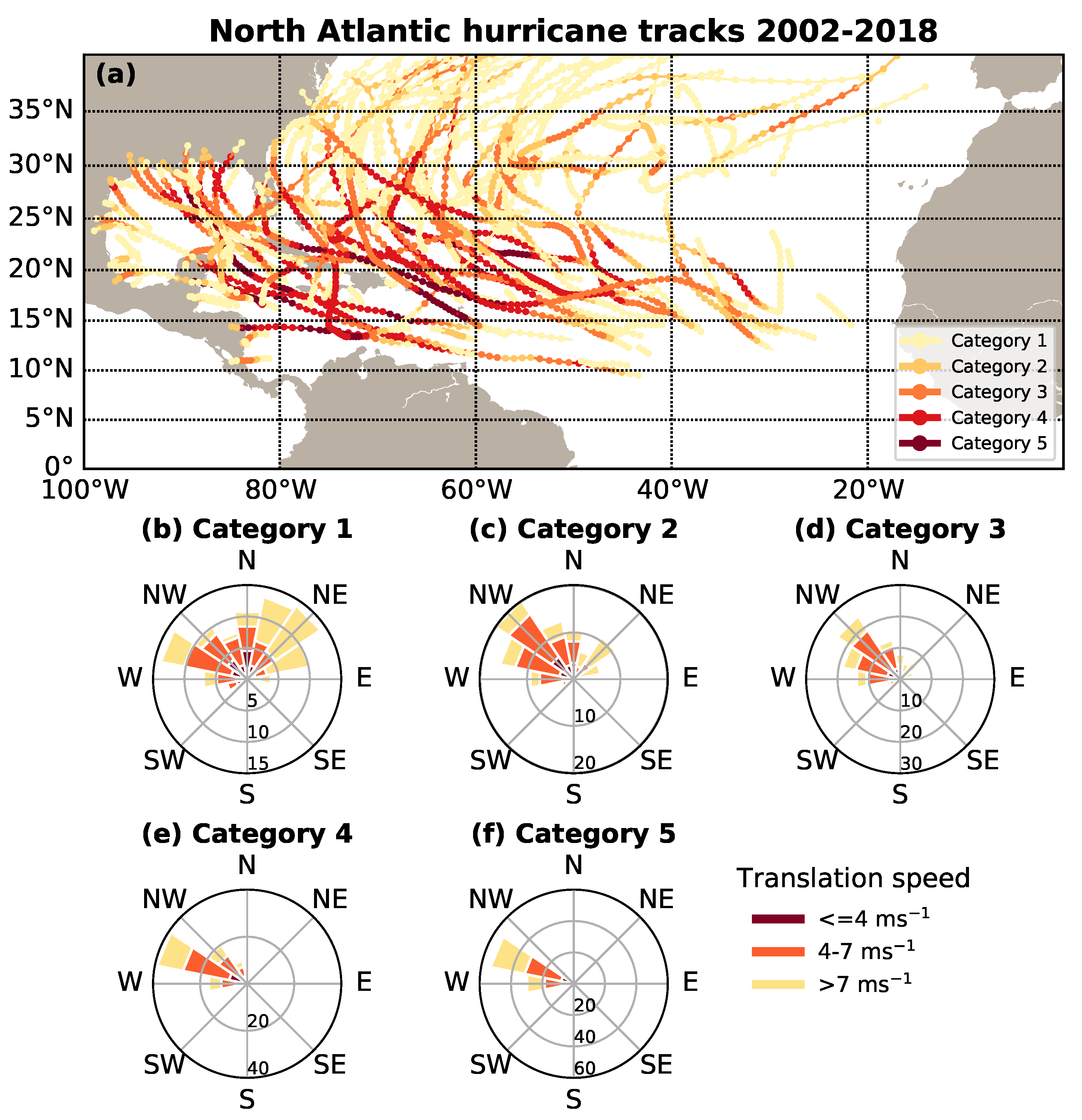
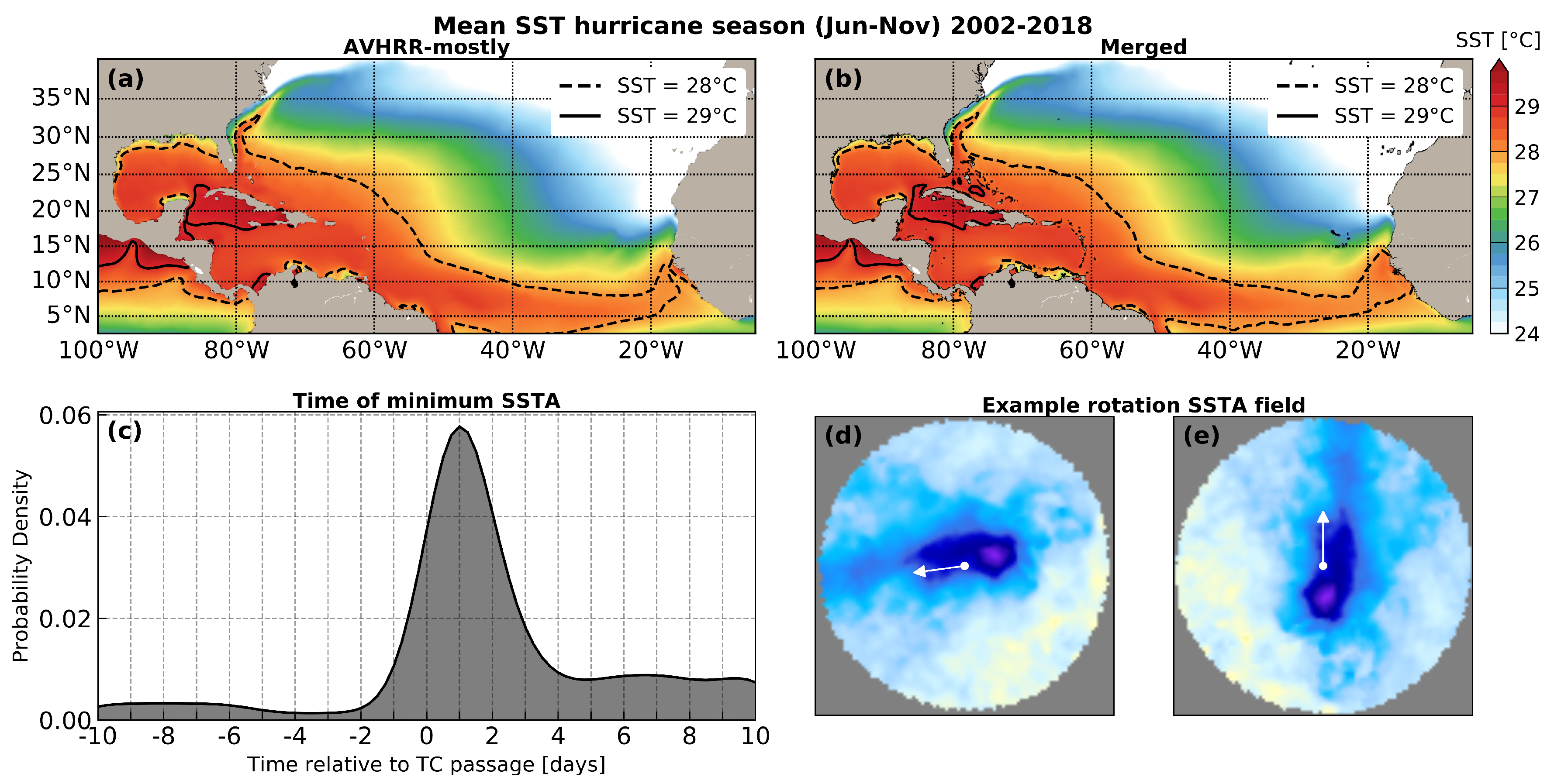
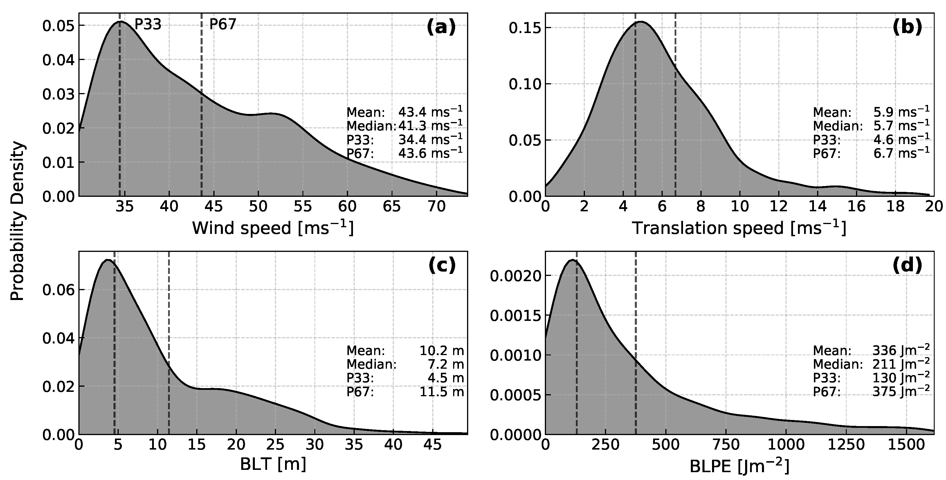
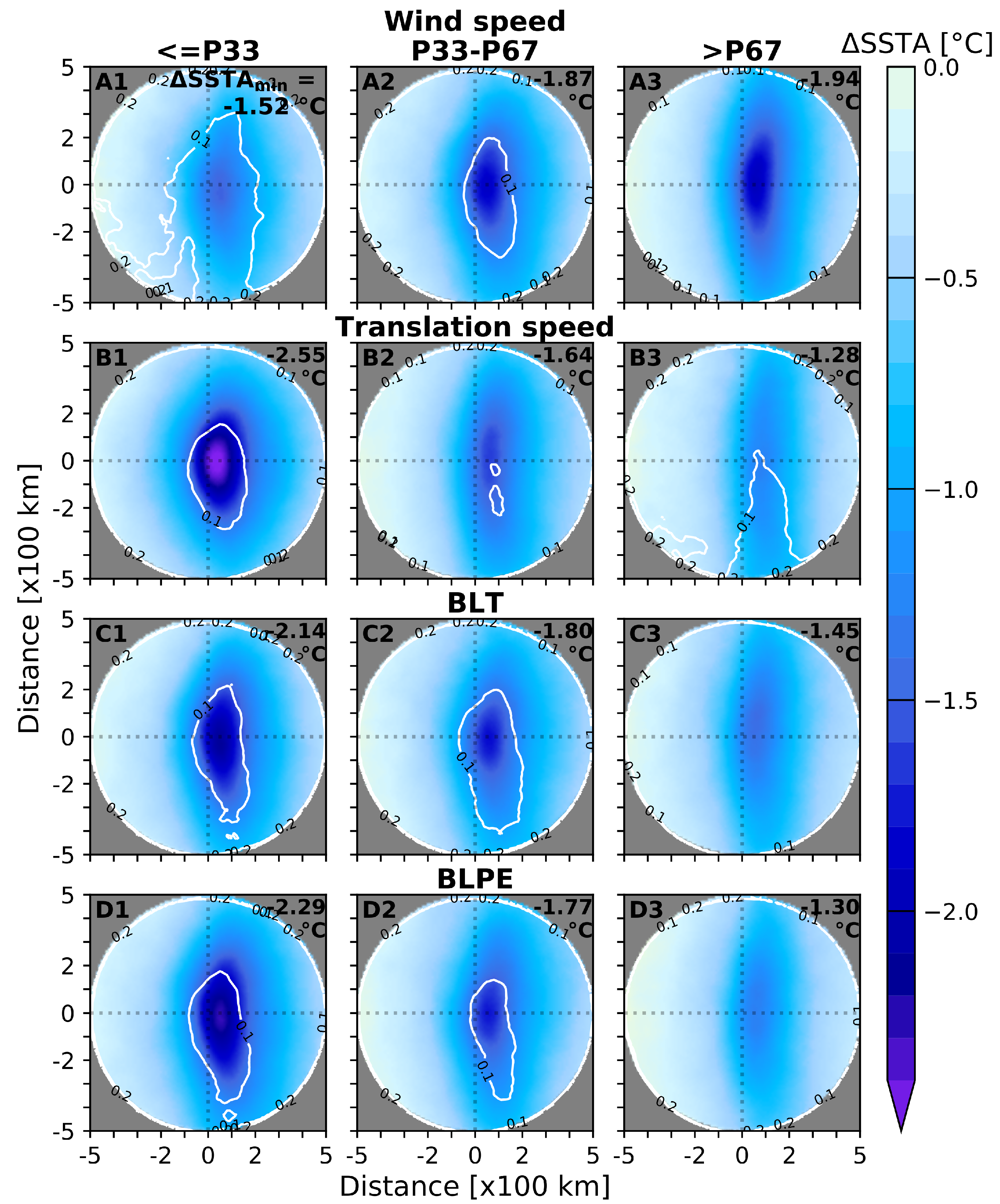
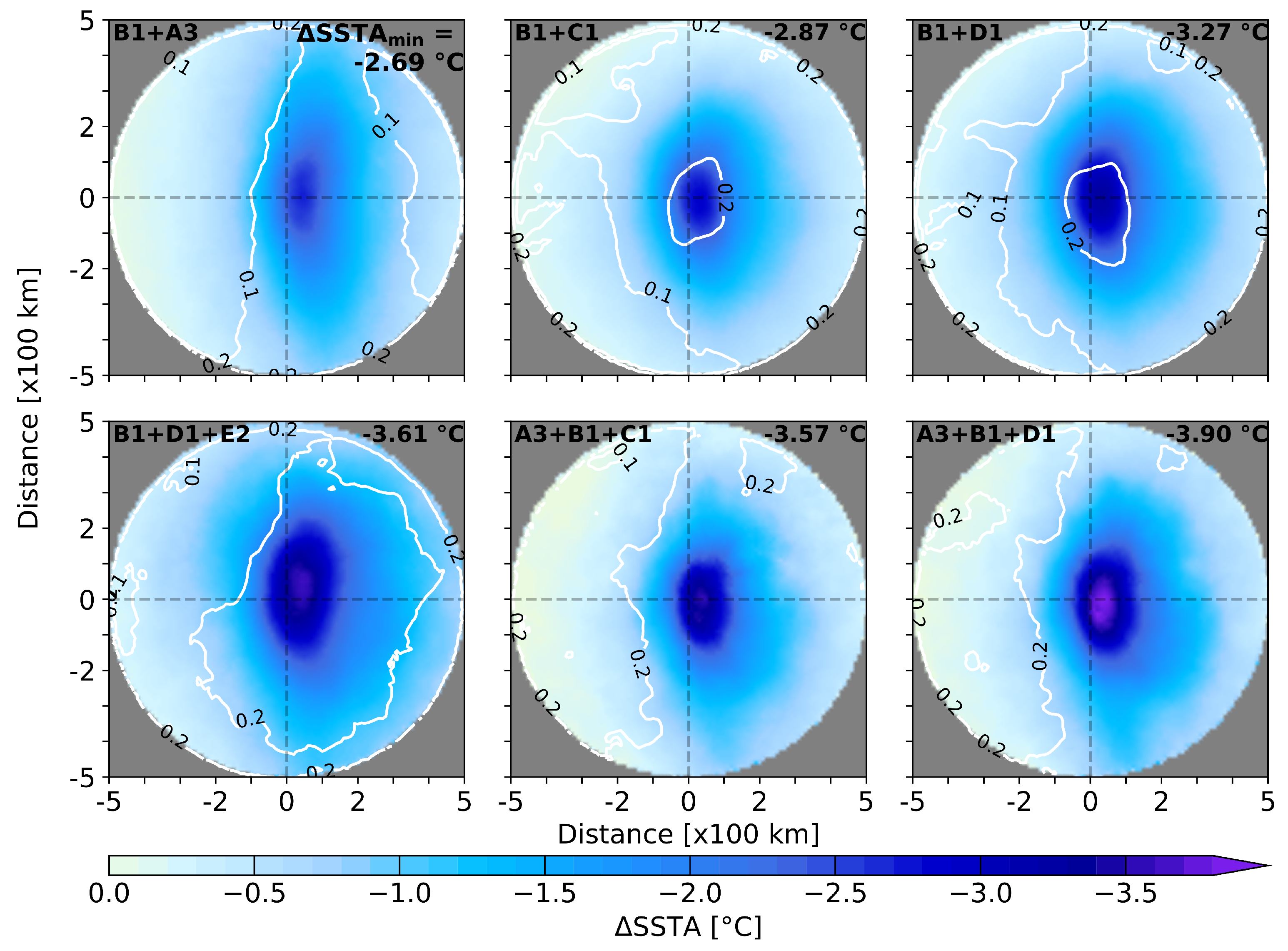
Table 1.
Comparison between the mean cold wake composites of AVHRR-mostly and merged SST datasets. N refers to the number of observations. is the minimum SSTA, is the spatial average of SSTA over a centered disk of 200 km of radius, which includes the kernel of the cold wake (the region with largest SST gradients), is the position of along the x-axis (at ), is the position of along the y-axis (at ), (column seven) is the width of the cold wake (illustrated by colored triangles in Figure 5m,n), which we have defined as the e-folding spatial decay along the x-axis, i.e., the distance between the two points on the curve on the x-axis where . Uncertainties for all values of , and are of 10 km, as stated by the grid resolution of the interpolated mesh, which is a larger value than the margin of error.
| Category | Dataset | N | [°C] | [°C] | [km] | [km] | [km] |
|---|---|---|---|---|---|---|---|
| All | AVHRR-mostly | 1810 | 60 | −10 | 510 | ||
| merged | 1810 | 50 | −10 | 480 | |||
| 1 | AVHRR-mostly | 890 | 50 | −20 | 520 | ||
| merged | 890 | 40 | −10 | 530 | |||
| 2 | AVHRR-mostly | 260 | 60 | −10 | 530 | ||
| merged | 260 | 40 | −40 | 490 | |||
| 3–5 | AVHRR-mostly | 660 | 60 | 0 | 490 | ||
| merged | 660 | 50 | −20 | 420 |
Table 2.
Summary of the main cold wake composite results for individual parameters based on the merged SST dataset: 10-min maximum sustained wind speed (), the hurricane translational speed (), barrier layer thickness (BLT) and the barrier layer potential energy (BLPE). See Table 1 for a description of columns. Please note that the total number of observations is lower in comparison to Table 1, the reason is that some observations of BLT and/or BLPE are missing or present negative values (around 200 observations). These observations have not been taken into account in Section 4 and subsequent analysis.
| Category | Case | Definition | N | [°C] | [°C] | [km] | [km] | [km] |
|---|---|---|---|---|---|---|---|---|
| A1 | 460 | 50 | 0 | 540 | ||||
| A2 | 535 | 50 | −10 | 490 | ||||
| A3 | 596 | 50 | −20 | 420 | ||||
| B1 | 515 | 40 | −10 | 450 | ||||
| B2 | 580 | 60 | −20 | 490 | ||||
| B3 | 496 | 80 | 30 | 480 | ||||
| BLT | C1 | 531 | 50 | 10 | 440 | |||
| C2 | 530 | 60 | 50 | 510 | ||||
| C3 | 530 | 50 | −10 | 490 | ||||
| BLPE | D1 | 531 | 50 | 10 | 460 | |||
| D2 | 530 | 50 | 30 | 510 | ||||
| D3 | 530 | 50 | −10 | 460 |
Table 3.
Summary of the cold wake composite obtained from the merged SST dataset that shows the strongest cooling when the synergistic effect of two or three parameters is considered. All cases were defined in Table 2 except E2, which refers to those hurricane observations between a latitude band of 20–30°N. See Table 1 for a description of columns.
| Case | N | [°C] | [°C] | [km] | [km] | [km] |
|---|---|---|---|---|---|---|
| B1+A3 | 177 | 50 | −10 | 390 | ||
| B1+C1 | 187 | 40 | −20 | 380 | ||
| B1+D1 | 179 | 40 | −20 | 420 | ||
| A3+B1+C1 | 38 | 40 | −10 | 320 | ||
| A3+B1+D1 | 29 | 40 | 0 | 340 | ||
| B1+D1+E2 | 66 | 40 | −20 | 480 |
Table 4.
Relationship between hurricane and ocean properties and hurricane intensification for four categories: NR (neutral response), RI (rapid intensification), SI (slow intensification) and WK (weakening). The definition of each category is described in the second column considering the variation of (referred to as ) and unit of kt/24h (). is the mean hurricane moving speed and the mean hurricane latitude. The asterisk (*) indicate those values that present a significant difference (at 95%, based on Welch’s unpaired t-test), with respect to the corresponding NR values. SST is derived from the merged SST dataset.
| Cat | Definition [] | # | [] | [°C] | [°C] | [m] | [] | [deg] | [] |
|---|---|---|---|---|---|---|---|---|---|
| WK | 503 | * | * | ||||||
| NR | 634 | ||||||||
| SI | 232 | * | * | * | * | ||||
| RI | 90 | * | * | * | * |
© 2019 by the authors. Licensee MDPI, Basel, Switzerland. This article is an open access article distributed under the terms and conditions of the Creative Commons Attribution (CC BY) license (http://creativecommons.org/licenses/by/4.0/).
Share and Cite
MDPI and ACS Style
Haakman, K.; Sayol, J.-M.; van der Boog, C.G.; Katsman, C.A. Statistical Characterization of the Observed Cold Wake Induced by North Atlantic Hurricanes. Remote Sens. 2019, 11, 2368. https://0-doi-org.brum.beds.ac.uk/10.3390/rs11202368
AMA Style
Haakman K, Sayol J-M, van der Boog CG, Katsman CA. Statistical Characterization of the Observed Cold Wake Induced by North Atlantic Hurricanes. Remote Sensing. 2019; 11(20):2368. https://0-doi-org.brum.beds.ac.uk/10.3390/rs11202368
Chicago/Turabian StyleHaakman, Koen, Juan-Manuel Sayol, Carine G. van der Boog, and Caroline A. Katsman. 2019. "Statistical Characterization of the Observed Cold Wake Induced by North Atlantic Hurricanes" Remote Sensing 11, no. 20: 2368. https://0-doi-org.brum.beds.ac.uk/10.3390/rs11202368
Note that from the first issue of 2016, this journal uses article numbers instead of page numbers. See further details here.