Monitoring Harvesting by Time Series of Sentinel-1 SAR Data


Earth Observing System, 1906 El Camino Real, Suite 201, Menlo Park, CA 94027, USA
*
Author to whom correspondence should be addressed.
Remote Sens. 2019, 11(21), 2496; https://0-doi-org.brum.beds.ac.uk/10.3390/rs11212496
Submission received: 19 September 2019
/
Revised: 22 October 2019
/
Accepted: 23 October 2019
/
Published: 25 October 2019
(This article belongs to the Section Remote Sensing in Agriculture and Vegetation)
Abstract
:Algorithm for determining crop harvesting dates based on time series of coherence and backscattering coefficient () derived from Sentinel-1 single look complex (SLC) synthetic-aperture radar (SAR) images is proposed. The algorithm allows the ability to monitor harvesting over large areas without having to install additional sensors on agricultural machinery. Coherence between SAR images allows the ability to track changes in field-scatterers configuration resulting from agricultural work. The proposed algorithm finds a step-like increase in coherence that occurs after the harvesting and is related to the conversion of a field into a bare soil area. An additional check of potential harvest dates is carried out by threshold values of depending on vegetation height. The algorithm is adapted for the monitoring of non-homogeneous fields with traces of erosion and insertions of fallow land. The algorithm was tested on agricultural fields located in the north of Kazakhstan. The obtained accuracy (mean absolute error = 6.5 days) of determining the dates of harvesting can be deemed satisfactory. This accuracy can be increased by shortening the interval between observations from 12 to 6 days when using data from both Sentinel-1 satellites.

1. Introduction
Ground, unmanned aerial vehicle (UAV) and global positioning system (GPS) satellite observations over the agricultural machinery are widely used for monitoring of harvesting [1,2]. Installation of various sensors allows to monitor position, velocity and other meaningful parameters of harvesters in real time. A necessary component of such monitoring systems is geoinformation system (GIS) enabling tracking of harvesters’ operation within the boundaries of fields. A limitation of this approach is the high cost of sensors installation, reception and processing of their readings as well as development and maintenance of a special GIS.
An irreplaceable instrument in monitoring large areas of crops is satellite remote sensing data. Freely available satellite data are attractive to farmers with low budgets in particular. For implementation of the monitoring, it is necessary to cover the investigated area with the satellite data enabling reliable detection of the fact of harvesting.
Analysis of the possibility of monitoring harvesting using optic sensor data showed that after harvesting a striped texture appears with spatial dimensions corresponding to the swath of the harvester (usually, 6 to 9 m) [3]. Such textures are reliably registered in high spatial resolution images (up to 10 m). Raking of straw forms another texture related to a pattern of stacks or traces of their collection and removal from the field. The spatial scale of this texture is determined by the distance between rows of straw stacks. Textures formed by the raking of straw are well discerned in medium-resolution images (30 m). In low-resolution images, such as moderate resolution imaging spectroradiometer (MODIS) data, neither of these textures are discernible.
Low-resolution satellite data can register a change in averaged values of reflection coefficients of the field or vegetation indexes. Harvesting may either increase or decrease these values [3]. According to Muratova et al. [3], quantitative characteristics of changes depend on the volume of plant biomass before harvesting, the method of harvesting and the make of the harvester. As a result, time series of data from low-resolution optic sensors are not suitable for determining dates of harvesting.
A number of works [4,5,6,7] are devoted to the determination of dates of phenological phases change with the use of a time series of optic sensors data. By determining the moment of the end of the vegetation season (EOS, the end of the growing season) related to the ripening of plants, it is possible to forecast the time of harvesting. However, it is impossible to detect harvesting using this approach.
Thus, for detection of harvested fields, it is preferable to use optical data of medium and high resolution (5 to 10 m). The monitoring of harvesting with such images is concerned with the problem that is inevitably linked to limitations of cloud cover. A possibility of observation irrespective of clouds is provided by radar data.
Spaceborne radar imaging provides valuable information about the condition of the earth’s surface, in particular, vegetation cover. The main advantage of radar data in comparison with the data from optical sensors is independence from cloudiness and solar illumination of the surface area under consideration. Independency from cloud cover allows for reliable image acquisitions at regular intervals which is decisive for agricultural applications.
Synthetic-aperture radar (SAR) image is based on peculiarities of backscattering of the emitted radar signal by surfaces of different kinds [8]. The radar backscattering coefficient (“sigma nought”) is a fraction which describes the amount of average backscattered power compared to the power of the incident field [9]. The value of is a function of the radar observation parameters: frequency, polarization, incidence angle of the emitted electromagnetic waves; physical (roughness and the area relief) and dielectric properties of the investigated surface [9,10].
When treated in terms of agricultural problems, plantations of agricultural crops and open ploughed soil function as a surface [8,11,12]. The resulting intensity of the radar signal reflection is influenced by biophysical characteristics of the vegetation, such as sowing density, stalks height, and the size and position of leaves. Since observation is conducted with a significant angle of deviation from nadir, value is affected even by the direction of ploughing. Thus, a complex character of interaction between the radar signal and the surface is a challenge for a modern researcher in terms of interpretation of the investigated field state.
A simple “cloud” model that provides a clue for understanding the relationships between and the state of soil and vegetation was developed in the late 1970s [13]. The possibilities of using SAR data for agricultural applications were actively studied in the late 1980s.
Considering the related literature review [8,10,11], most published works devoted to the monitoring of vegetation with the use of radar, characterize the interaction of the signal with the surface by the backscattering coefficient . Recent publications [14,15,16] also use as the main indicator of plants state. Interpretation of the time series from the point of view of events occurring in the field yields ambiguous results: An increase in can be caused by growth of plants, precipitation or cultivation of soil [15,16]. For eliminating this ambiguity, additional data should be involved, for instance, information on precipitation.
Valuable information about the vegetation state can be obtained from coherence [17]. Coherence is the modulus of the complex coefficient related to correlation between two single look complex (SLC) images containing information on the amplitude and phase of the radar signal. Coherence will be high when two interfering images reveal the same or almost the same interaction with the scattering surface. Change of at high coherence of images indicates change of dielectric permittivity of the surface at unchanged layout of scatterers in the field [18,19] (for instance, because of increased moisture in the soil due to precipitation). On the other hand, stable values of accompanied by low coherence indicate a change in configuration of scatterers. This can result from the field tillage or harvesting—agricultural operations which change the state of the soil upper layer or the vegetation cover but produce little influence on dielectric properties of the soil.
Combined use of and coherence for monitoring of vegetation is analyzed in a relatively small number of works [18,19,20,21,22,23]. Snapir et al. [21] describes detection of harvested tea fields with the use of coherence. According to Khabbazan et al. [23], the sudden increase in coherence is a useful indicator of harvest. Kavats et al. [22] considers a possibility to detect sowing and harvesting dates with the use of time series of and coherence.
The present paper aims to develop results of the [22] research by proposing the method for detection of the harvesting end date. The idea of the proposed method is based on the property of radar images coherence. The periods when fields are covered with thick vegetation or when agricultural works are performed on them, are characterized by low coherence. On the contrary, a harvested field can be considered as an area of bare land or rarefied vegetation, for which high coherence is typical. Thus, the end of harvesting on a field is accompanied by an abrupt increase in coherence. This moment is proposed for detection.
2. Materials and Methods
2.1. Study Area
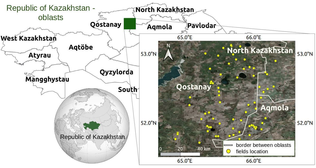
Study area is located in northern Kazakhstan in the Aqmola and Qostanay Oblasts (Figure 1). Kazakhstan is one of the world’s largest exporters of wheat (the 10th place in 2018, 2.3% of world exports) [24]. The main wheat sown areas are located in the northern part of the country, in Aqmola and Qostanay Oblasts. In 2018, 74% of sown areas in Aqmola Oblast and 67% in Qostanay Oblast were cultivated with wheat [25]. The climate of northern Kazakhstan is harsh continental with an average temperature from °C to °C in January and from °C to °C in July. In winter, the temperature may fall to °C, and in summer it is up to °C. Due to harsh winters, spring crops dominate in northern Kazakhstan [26]. The main crops are spring cereals, among which wheat predominates. According to the crop calendar, sowing in study areas occurs in the second half of May, and harvesting is in August–September [26].
A characteristic peculiarity of the observed areas is their heterogeneity caused by erosion of soil, presence of fragments of lea and fallow and the presence of weed vegetation and inaccuracies of delimitation (Figure 2).
2.2. Harvesting Dates
Harvesting dates in the areas were initially determined by visual decoding of Sentinel-2 and Landsat-8 images obtained from the EOS land viewer service [27]. Observation periodicity by Sentinel-2 satellites in the area under consideration was about 3 days. For testing, we selected the fields whose images present the complete process of harvesting—from beginning to end. The date of the last image was deemed to mark the end of harvesting (Figure 3). Thus, the error of harvesting date detection does not exceed 3 days, and sometimes even less—due to Landsat-8 images. As a result, the algorithm quality was tested on a sample of 77 fields located in Aqmola and Qostanay Oblasts.
2.3. Satellite Data
Time series of Sentinel-1B SLC Interferometric Wide (IW) images (relative orbit 20, slice 4, swath IW2) were used to detect harvesting over the study area. Images were sensed every 12 days from 1 May 2018 to 28 October 2018 (image of 5 August 2018 is absent) and were taken from Copernicus Open AccessHub [28].
Harvesting is performed in the generative period of a plants development. This period can be detected by the reduction of the normalized difference vegetation index (NDVI) in the field to a particular level of the maximum seasonal values achieved at the peak of plants vegetation. NDVI time series were built based on the 8 day MOD09Q1 composites [29]. Images for the period 7 April 2018–1 November 2018 were used.
For estimating the changes of due to precipitation, global precipitation measurement (GPM) data were used, namely integrated multi-satellite retrievals for GPM (IMERG) with a 30 min period of precipitation accumulation [30]. The interval of observations were 27 April 2018–November 2018. Data on precipitation in liquid and mixed phases were used. A structural diagram presenting all data sources and work flows of this approach is presented in Section 3 (Figure 5).
2.4. Processing
The backscattering coefficient and coherence were computed with European Space Agency (ESA) Sentinel Application Platform (SNAP) software v. 6.0 [31]. Computing was automated with Graph Processing Tool (GPT) and bash scripts (Figure 4).
The MOD09Q1 images were downloaded and processed with instruments of the MODIStsp library [32] in the R package [33]. Time series of NDVI averaged over the area were built and smoothened with spline interpolation (smooth.spline function).
If, according to GPM IMERG Late data, precipitation of over 2 mm occurred up to 12 h before imaging, values of the respective date were considered unusable and were replaced by means of linear interpolation.
2.5. Control Points
To reduce the influence of row-spacing and inaccuracies of delimitation, a 15 m wide internal buffer zone was built around each field. For obtaining homogeneous fragments, control points were chosen randomly (spsample function of the sp package, option “stratified” [34]) inside the field and buffers of 100 m in radius were built around them. At least 30 such points were chosen for each field.
2.6. Monitoring Period
Spring cereal crops—mainly, wheat—prevail in the considered areas. For determining the time of the monitoring commencement, the date of NDVI maximum was registered, which approximately corresponds to the period of earing/flowering of the plants. This phase lasts for 7–10 days [35], then the ripening of the grains begins. Basing on the estimations of the ripening period beginning obtained with the use of NDVI, the gathering of radar data began on 1 August for the purpose of obtaining at least two coherence maps by the beginning of harvesting. The 2018 harvesting campaign in the considered region started at the beginning of September.
2.7. Accuracy Assessment
The errors in detecting the harvesting dates were estimated by mean absolute error (MAE) and root mean square error (RMSE),
where n–number of plots; –known date of harvesting the i-th plot; –date of harvesting the i-th plot determined by the algorithm.
3. Proposed Algorithm
For observation of harvesting, time series in vertical transmit and horizontal receive (VH) polarization () were used, because of the known high correlation between scattering in cross-polarization and indicators of the state of the plants’, such as leaf area index (LAI) [36,37]. Also VH backscatter is in general more sensitive to vegetation volume scattering [15]. Coherence maps were built for the vertical transmit and vertical receive (VV) polarization (), because coherence in the VH polarization proved to be less sensitive to the changes occurring in the field [22].
Time series of averaged values and were built for each control point.
The stages of the algorithm are shown in Figure 5.
The key stage of the algorithm is the determination of the date of harvesting completion for a control point. Strictly speaking, the creation of a control point relates to the specific implementation of the algorithm for the territory of North Kazakhstan. Estimations carried out previously for Ukraine in Kavats et al. [22] showed that, in homogeneous areas, the choice of control points is not necessary, and values of and coherence averaged over an area suffice. Thus, for homogeneous fields, the control point is the entire field. Further, NDVI time series help to more accurately determine the moment of observations commencement and thus save computing resources, but the use of these series is not compulsory.
Determination of the harvesting date for a control point includes:
- Registration of harvesting completion dates by changes in coherence;
- Filtering of false triggering by the threshold values of .
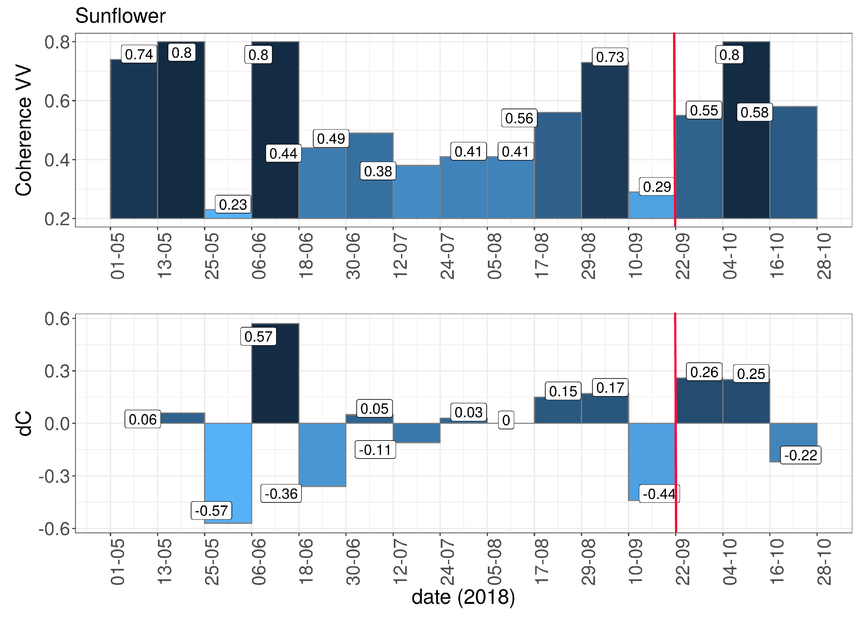
Let us consider how the harvesting end dates are searched for by changes in the coherence time series (Figure 6 and Figure 7). Soybean and sunflower fields were chosen as a good example of determining the harvesting end dates.
Observations showed that the coherence time series in the period of ripening behaves in one of the following ways [22]:
- Coherence is gradually increasing as the plants are ripening and drying out (Figure 6, 5 August–10 September 2018). Then, coherence drops, typically, during the period of harvesting (Figure 6, 10–22 September 2018). After that, coherence is growing again (Figure 6, 22 September–4 October 2018). In particular, such behavior is observed in row crops.
Figure 8 illustrates the general pattern of coherence changes during the cereals harvesting period. The coherence is high before harvesting (Figure 8a,b), then steeply decreases to the minimum values during the harvesting (Figure 8c) and increases again when agricultural field is harvested (Figure 8d). The flowchart of harvesting date determining for a control point is shown in Figure 9.
Let be an i-th coherence map and n–the total number of such maps. Let us calculate the differences of coherence and determine the trend of their change. We will choose such a threshold that at changes of within the range the coherence is deemed constant ().
Harvesting corresponds to a drop of coherence () or unchanged coherence () in comparison with the previous period. After the harvesting, coherence should grow (). Thus, harvesting corresponds to transitions : or . Introducing second differences , we will write the condition for the change of coherence corresponding to harvesting
Note that transition from to 0 also yields . In some cases, this moment can correspond to the beginning of harvesting, but not to its end. Therefore, an additional check is introduced: the second date in the transition should satisfy the condition of .
After checking conditions (Equation (4)), one or several possible dates of harvesting are assigned to each control point. The next step is checking these dates by the threshold values of –the threshold of dense vegetation () and the threshold of bare soil (). If, at a given control point on a verified date, the vegetation remained sufficiently dense (), this jump of coherence is not considered as related to harvesting. Such date is excluded from the list of possible harvesting dates. If, upon a given date, the field has been harvested to the state of bare soil (), then check of subsequent dates becomes unnecessary.
The earliest of the dates which remained in the list after checking is assumed to be the date of the end of harvesting at a given control point. Later dates may be related to works after harvesting, for instance, disk harrowing.
A conclusion about the harvesting date of the whole area is made after achievement of a particular threshold of the number of harvested control points. For instance, if 70% of points have been harvested by a given date, the area has been harvested. Thus, the last parameter of the algorithm is —the share of the control points that obtained harvesting dates, which is sufficient for considering the area harvested.
4. Results and Discussion
The algorithm results are demonstrated by the example of grain crops harvesting in Fyodorov District of Qostanay Oblast. It was found that agricultural fields were harvested from August to October 2018. The harvesting dates (3 August 2018, 15 August 2018, 21 August 2018, 8 September 2018, 20 September 2018, 2 October 2018, 14 October 2018) correspond to Sentinel-1 sensing dates (Figure 10).
Harvesting monitoring was carried out for 1920 fields with a total area of 471,903 ha. Among them, 221 fields are defined as non-harvestable (vapors, pastures, hayfields, etc.), and 51 fields were not harvested—class “other” in Figure 10. By mid-October, 1648 fields with a total area of 395,877 ha were harvested, including by month:
- in August—572 fields.
- in September—1010 fields.
- in October—66 fields.
The harvesting completion dates were computed with the following parameters of the algorithm: , dB, dB, . Beginning of the monitoring: 1 August 2018, end of the monitoring: 1 November 2018.
The accuracy assessment gave the following error values: MAE = 6.5 days, RMSE = 8.0 days.
The following particularities of and coherence time series, typical for grain crops in the north of Kazakhstan, were taken into account when searching for harvesting end dates:
- is low at least in one of the first sensing dates (sometimes in two or three dates). This allows the ability to determine the beginning of sowing period and presowing treatment.
- The last of the low values at the beginning of the growing season corresponds to sowing. After sowing increases abruptly.
- The maximum values during the growing season are from to dB.
- High values (>0.4) are possible during the growing season, and cannot be explained by incidence angle effect (the incidence angle would affect the average coherence during the entire season). Such fields contain sparse vegetation and/or row crops with wide planting distances.
- As a rule, no more than one alternation of low-high with a small amplitude is observed for grain crops during plant growth. The decrease in down to 0.3 disrupting a smooth U-trend during the growing season is caused by soil cultivation. Coherence never decreases to an open soil level of 0.25.
The main factor influencing the accuracy of harvesting completion dates computation is the imaging periodicity of Sentinel-1 satellites. Currently, the revisiting period is 12 days (the study area is fully covered by Sentinel-1B satellite data). The accuracy can be increased by reducing the interval between imaging from 12 to 6 days owing to involvement of data from both Sentinel-1 satellites. However, judging by the archive data and imaging schedules [38], this is an unlikely option in the studied area.
It should be noted that the dates of harvesting for the investigated agricultural fields were obtained by visual interpreting and, therefore, they can differ from the actual harvesting dates by 1 to 3 days, which is related to the periodicity of imaging by satellites Sentinel-2A, B and Landsat-8, and to the presence of cloudiness.
Coherence is usually high after harvesting [23]. However agrotechnical works, which are accomplished soon after harvesting and cause changes of the soil upper layer, decrease coherence and are registered by the algorithm as a part of harvesting works. For instance, if, in the 12 day interval after harvesting, disk harrowing is done, the date of disking is registered as the date of harvesting. Thereby the harvesting end date determined by the algorithm will be later than the actual harvesting end date. An increase in frequency of imaging could help to solve this problem.
It can be assumed that MAE is equal to the half interval between sensing dates (6 days). However, considering the above, the obtained accuracy of the harvesting date determination can be regarded as satisfactory.
Omissions of individual images and periodic planned omissions of whole relative orbits represent a problem for monitoring. Omission of a single image in a time series in the period of ripening can substantially reduce accuracy of harvesting completion date determination. This brings about a problem of the omitted images interpolation. Linear interpolation of the coherence results in missing the jumps of coherence, while step interpolation causes false triggering of the algorithm. In our case, step interpolation was used for filling-in the omitted coherence values on 5 August 2018. Cases of false triggering were removed via checking by the threshold. For filling-in omissions of , a linear interpolation was used.
The coherence may increase steeply before harvesting. Presumably, they are related to vegetation water content (VWC) decrease and leafage area reduction [14,15,23]. False triggering of the algorithm in such cases is prevented by checking () values.
Sometimes harvesting end date could not be found because the coherence increases too slightly after harvesting. Such cases were related to the fields, whose dates of harvesting were supposed to be found by the algorithm on 22 September 2018. It may have been the result of a heavy rain observed on that day, according to the GPM IMERG data, shortly before sensing. Presumably, the rain caused decrease of coherence (a similar effect is reported in [23]), which made it impossible to register its steep increase expected after the end of harvesting. The effect of rains on the is well-known [16,39], however, their influence on the coherence is less pronounced. This case requires additional research.
The algorithm can be improved in several ways. Additional harvesting features can be obtained using surface texture characteristics [16]. Clustering using NDVI or other features derived from optical data seems to be a more advanced way to detect homogeneous fragments within an agricultural field.
5. Conclusions
An algorithm of harvesting completion dates determination by time series of and coherence is proposed. The algorithm registers a step-like growth of coherence which appears after harvesting and is related to the field transformation into the area of bare land. Harvesting potential dates are additionally verified by value.
The algorithm is adapted for monitoring of non-homogeneous fields (with marks of erosion and fragments of fallow land). For this purpose, it is proposed to determine the date of harvesting of small homogenous parts within the field (control points) and to decide upon the date of the field harvesting by the date of harvesting most of such parts of the field. For homogeneous fields, time series of and coherence averaged over the field are used.
Errors in determining the harvesting completion dates are: MAE = 6.5 days, RMSE = 8.0 days.
Omissions in the time series of Sentinel-1 SLC IW data corresponding to the period of ripening reduce accuracy of determining the date of harvesting completion. Increase in the accuracy can be achieved by shortening the interval between acquisitions of images from 12 to 6 days by using both Sentinel-1 satellites.
The proposed algorithm is used by the Earth Observing System company.
Author Contributions
All authors contributed significantly to this manuscript. V.V. designed this study. O.K., K.S. and D.K. were responsible for the data processing, analysis, and paper writing. D.K. developed and implemented the software. All authors reviewed the manuscript.
Funding
This research received no external funding.
Acknowledgments
The authors would like to express their sincere gratitude to the Earth Observing System company (eos.com) and its Chief Executive Officer, President Max Polyakov for his support, development and kind assistance with this study. We are also grateful to reviewers and editors for their valuable comments, recommendations, and attention to the work.
Conflicts of Interest
The authors declare no conflict of interest.
Abbreviations
The following abbreviations are used in this manuscript:
| ESA | European Space Agency |
| GIS | Geoinformation system |
| GPM | Global Precipitation Measurement |
| GPS | Global Positioning System |
| GPT | Graph Processing Tool |
| IMERG | Integrated Multi-satellitE Retrievals for GPM |
| IW | Interferometric Wide |
| LAI | Leaf area index |
| MAE | Mean absolute error |
| MODIS | Moderate Resolution Imaging Spectroradiometer |
| NDVI | Normalized Difference Vegetation Index |
| RMSE | Root Mean Square Error |
| SLC | Single Look Complex |
| SNAP | Sentinel Application Platform |
| UAV | Unmanned aerial vehicle |
| VH | Vertical transmit and horizontal receive |
| VV | Vertical transmit and vertical receive |
| VWC | Vegetation water content |
References
- Xiang, M.; Wei, S.; Zhang, M.; Li, M. Real-time Monitoring System of Agricultural Machinery Operation Information Based on ARM11 and GNSS. IFAC-PapersOnLine 2016, 49, 121–126. [Google Scholar] [CrossRef]
- Kunal, S.; Singh, S.; Rana, R.S.; Rana, A.; Vaibhav, K.; Kaushal, A. Application of GIS in Precision Agriculture. 2015. Available online: https://www.researchgate.net/profile/Kunal_Sood4/publication/295858552_Application_of_GIS_in_precision_agriculture/links/573eedd408ae298602e8e432.pdf (accessed on 24 October 2019).
- Muratova, N.; Terekhov, A. Tekhnologiya uborki zernovykh kul’tur Kazakhstana v predstavlenii sputnikovykh dannykh. Sovremennye Problemy Distantsionnogo Zondirovaniya Zemli iz Kosmosa 2007, 4, 269–276. [Google Scholar]
- Sakamoto, T.; Yokozawa, M.; Toritani, H.; Shibayama, M.; Ishitsuka, N.; Ohno, H. A crop phenology detection method using time-series MODIS data. Remote Sens. Environ. 2005. [Google Scholar] [CrossRef]
- You, X.; Meng, J.; Zhang, M.; Dong, T. Remote Sensing Based Detection of Crop Phenology for Agricultural Zones in China Using a New Threshold Method. Remote Sens. 2013, 5, 3190–3211. [Google Scholar] [CrossRef] [Green Version]
- Zheng, Y.; Wu, B.; Zhang, M.; Zeng, H. Crop Phenology Detection Using High Spatio-Temporal Resolution Data Fused from SPOT5 and MODIS Products. Sensors 2016, 16, 2099. [Google Scholar] [CrossRef] [PubMed]
- Lin, C.H.; Liu, Q.S.; Huang, C.; Liu, G.H. Monitoring of winter wheat distribution and phenological phases based on MODIS time-series: A case study in the Yellow River Delta, China. J. Integr. Agric. 2016. [Google Scholar] [CrossRef]
- Riedel, T.; Eckardt, R. Agricultural Applications with SAR Data. Module 3202: Biosphere. Available online: https://saredu.dlr.de/unit/agriculture (accessed on 24 October 2019).
- Lusch, D. Introduction To Microwave Remote Sensing; Center For Remote Sensing and Geographic Information Science Michigan State University: East Lansing, MI, USA, 1999; p. 84. [Google Scholar]
- Ferrazzoli, P. SAR for Agriculture: Advances, Problems and Prospects. In Proceedings of the 3rd International Symposium on Retrieval of Bio- and Geophysical Parameters from SAR Data for Land Applications, Sheffield, UK, 11–14 September 2001. [Google Scholar]
- Brisco, B.; Brown, R. Agricultural Applications with Radar. In Principles & Applications of Imaging Radar. Manual of Remote Sensing, 3rd ed.; Henderson, F., Lewis, A., Eds.; Wiley & Sons: New York, NY, USA, 1998. [Google Scholar]
- Ballester-Berman, J.D.; Lopez-Sanchez, J.M.; Fortuny-Guasch, J. Retrieval of biophysical parameters of agricultural crops using polarimetric SAR interferometry. IEEE Trans. Geosci. Remote. Sens. 2005. [Google Scholar] [CrossRef]
- Attema, E.P.W.; Ulaby, F.T. Vegetation modeled as a water cloud. Radio Sci. 1978, 13, 357–364. [Google Scholar] [CrossRef]
- Vreugdenhil, M.; Wagner, W.; Bauer-Marschallinger, B.; Pfeil, I.; Teubner, I.; Rüdiger, C.; Strauss, P. Sensitivity of Sentinel-1 backscatter to vegetation dynamics: An Austrian case study. Remote Sens. 2018, 10, 1396. [Google Scholar] [CrossRef]
- Harfenmeister, K.; Spengler, D.; Weltzien, C. Analyzing temporal and spatial characteristics of crop parameters using Sentinel-1 backscatter data. Remote Sens. 2019, 11, 1569. [Google Scholar] [CrossRef]
- Taravat, A.; Wagner, M.; Oppelt, N. Automatic Grassland Cutting Status Detection in the Context of Spatiotemporal Sentinel-1 Imagery Analysis and Artificial Neural Networks. Remote Sens. 2019, 11, 711. [Google Scholar] [CrossRef]
- Wegmüller, U.; Werner, C. Retrieval of vegetation parameters with SAR interferometry. IEEE Trans. Geosci. Remote Sens. 1997. [Google Scholar] [CrossRef]
- Engdahl, M. Multitemporal InSAR in Land-Cover and Vegetation Mapping. Ph.D. Thesis, Aalto University, Espoo, Finland, 2013. [Google Scholar] [CrossRef]
- Blaes, X.; Defourny, P. Retrieving crop parameters based on tandem ERS 1/2 interferometric coherence images. Remote. Sens. Environ. 2003. [Google Scholar] [CrossRef]
- Tamm, T.; Zalite, K.; Voormansik, K.; Talgre, L. Relating Sentinel-1 Interferometric Coherence to Mowing Events on Grasslands. Remote Sens. 2016, 8, 802. [Google Scholar] [CrossRef]
- Snapir, B.; Waine, T.W.; Corstanje, R.; Redfern, S.; Silva, J.D.; Kirui, C. Harvest Monitoring of Kenyan Tea Plantations With X-Band SAR. IEEE J. Sel. Top. Appl. Earth Obs. Remote. Sens. 2018, 11, 930–938. [Google Scholar] [CrossRef]
- Kavats, A.; Khramov, D.; Sergieieva, K.; Vasyliev, V.; Kavats, Y. Geoinformation technology of agricultural monitoring using multi-temporal satellite imagery. In Proceedings of the ICAG 2018: 20th International Conference on Agriculture and Geoinformatics, Menlo Park, CA, USA, 14–15 June 2018. [Google Scholar]
- Khabbazan, S.; Vermunt, P.; Steele-Dunne, S.; Ratering Arntz, L.; Marinetti, C.; van der Valk, D.; Iannini, L.; Molijn, R.; Westerdijk, K.; van der Sande, C. Crop Monitoring Using Sentinel-1 Data: A Case Study from The Netherlands. Remote Sens. 2019, 11, 1887. [Google Scholar] [CrossRef]
- Wheat Exports by Country. Available online: http://www.worldstopexports.com/wheat-exports-country/ (accessed on 24 October 2019).
- Statistics of Agriculture, Forestry, Hunting and Fisheries. Main Indicators. Available online: http://stat.gov.kz/official/industry/14/statistic/7 (accessed on 24 October 2019).
- Country Brief on Kazakhstan. Available online: http://www.fao.org/giews/countrybrief/country.jsp?code=KAZ (accessed on 24 October 2019).
- Land Viewer | EOS—EOS Data Analytics. Available online: https://eos.com/landviewer/ (accessed on 24 October 2019).
- Copernicus Open Access Hub. Available online: https://scihub.copernicus.eu/dhus/#/home (accessed on 24 October 2019).
- MOD09Q1—MODIS/Terra Surface Reflectance 8-Day L3 Global 250m SIN Grid. Available online: https://ladsweb.modaps.eosdis.nasa.gov/missions-and-measurements/products/land-surface-reflectance/MOD09Q1/ (accessed on 24 October 2019).
- Huffman, G.; Bolvin, D.; Nelkin, E. Integrated Multi-SatellitE Retrievals for GPM (IMERG); Version 5B; NASA’s Precipitation Processing Center: Washington, DC, USA, 2018. [Google Scholar]
- Sentinel Application Platform (SNAP). Available online: https://step.esa.int/main/toolboxes/snap/ (accessed on 24 October 2019).
- Busetto, L.; Ranghetti, L. MODIStsp: An R package for automatic preprocessing of MODIS Land Products time series. Comput. Geosci. 2016, 97, 40–48. [Google Scholar] [CrossRef]
- R Core Team. R: A Language and Environment for Statistical Computing; R Foundation for Statistical Computing: Vienna, Austria, 2019; Available online: https://www.R-project.org/ (accessed on 24 October 2019).
- Pebesma, E.; Bivand, R.S. Classes and Methods for Spatial Data: The sp Package. 2005. Available online: https://cran.r-project.org/web/packages/sp/vignettes/intro_sp.pdf (accessed on 24 October 2019).
- Spaar, D. Zernovyye kul’tury (Vyrashchivaniye, Uborka, Dorabotka i ispol’zovaniye); ID OOO “DLV Agrodelo”: Moscow, Russia, 2008. [Google Scholar]
- Ferrazzoli, P.; Paloscia, S.; Pampaloni, P.; Schiavon, G.; Solimini, D.; Coppo, P. Sensitivity to microwave measurements to vegetation biomass and soil moisture content: A case study. IEEE Trans. Geosci. Remote Sens. 1992, 30, 750–756. [Google Scholar] [CrossRef]
- Macelloni, G.; Paloscia, S.; Pampaloni, P.; Marliani, F.; Gai, M. The relationship between the backscattering coefficient and the biomass of narrow and broad leaf crops. IEEE Trans. Geosci. Remote Sens. 2001, 39, 873–884. [Google Scholar] [CrossRef]
- Sentinel-1 Observation Scenario. Available online: https://sentinel.esa.int/web/sentinel/missions/sentinel-1/observation-scenario (accessed on 24 October 2019).
- Hobbs, S.; Ang, W.; Seynat, C. Wind and Rain Effects on SAR Backscatter from Crops. In Proceedings of the 2nd International Workshop on Retrieval of Bio- and Geophysical Parameters from SAR Data for Land Applications, ETEC, Noordwijk, The Netherlands, 21–23 October 1998. [Google Scholar]
Figure 1.
Location of the study area.

Figure 2.
Example of a heterogeneous field (Sentinel-2 satellite image, date of acquisition 26 September 2018).
Figure 2.
Example of a heterogeneous field (Sentinel-2 satellite image, date of acquisition 26 September 2018).

Figure 3.
Example of a harvested field (Sentinel-2 satellite image).

Figure 4.
Data processing chain of Sentinel-1 radar images.

Figure 5.
Stages of the algorithm for determining the date of a field harvesting.

Figure 6.
Example of vertical receive (VV) coherence time series and its first differences () for sunflower fields (Ukraine), harvesting: 10–22 September 2018.
Figure 6.
Example of vertical receive (VV) coherence time series and its first differences () for sunflower fields (Ukraine), harvesting: 10–22 September 2018.

Figure 7.
Examples of VV coherence time series and its first differences () for soybean fields (Ukraine), harvesting: 31 August–12 September 2016.
Figure 7.
Examples of VV coherence time series and its first differences () for soybean fields (Ukraine), harvesting: 31 August–12 September 2016.

Figure 8.
The general pattern of VV coherence changes during the cereals harvesting period (Kazakhstan), harvesting: 23 Augus–4 September 2019.
Figure 8.
The general pattern of VV coherence changes during the cereals harvesting period (Kazakhstan), harvesting: 23 Augus–4 September 2019.

Figure 9.
Flowchart of harvesting date determining for a control point.

Figure 10.
The cartogram of harvesting of areas in Fyodorov District of Qostanay Oblast (the Republic of Kazakhstan), 2018.
Figure 10.
The cartogram of harvesting of areas in Fyodorov District of Qostanay Oblast (the Republic of Kazakhstan), 2018.

© 2019 by the authors. Licensee MDPI, Basel, Switzerland. This article is an open access article distributed under the terms and conditions of the Creative Commons Attribution (CC BY) license (http://creativecommons.org/licenses/by/4.0/).
Share and Cite
MDPI and ACS Style
Kavats, O.; Khramov, D.; Sergieieva, K.; Vasyliev, V. Monitoring Harvesting by Time Series of Sentinel-1 SAR Data. Remote Sens. 2019, 11, 2496. https://0-doi-org.brum.beds.ac.uk/10.3390/rs11212496
AMA Style
Kavats O, Khramov D, Sergieieva K, Vasyliev V. Monitoring Harvesting by Time Series of Sentinel-1 SAR Data. Remote Sensing. 2019; 11(21):2496. https://0-doi-org.brum.beds.ac.uk/10.3390/rs11212496
Chicago/Turabian StyleKavats, Olena, Dmitriy Khramov, Kateryna Sergieieva, and Volodymyr Vasyliev. 2019. "Monitoring Harvesting by Time Series of Sentinel-1 SAR Data" Remote Sensing 11, no. 21: 2496. https://0-doi-org.brum.beds.ac.uk/10.3390/rs11212496
Note that from the first issue of 2016, this journal uses article numbers instead of page numbers. See further details here.