Article

Mapping Photosynthesis Solely from Solar-Induced Chlorophyll Fluorescence: A Global, Fine-Resolution Dataset of Gross Primary Production Derived from OCO-2

Earth Systems Research Center, Institute for the Study of Earth, Oceans, and Space, University of New Hampshire, Durham, NH 03824, USA
*
Author to whom correspondence should be addressed.
Remote Sens. 2019, 11(21), 2563; https://0-doi-org.brum.beds.ac.uk/10.3390/rs11212563
Submission received: 2 September 2019 / Revised: 27 October 2019 / Accepted: 28 October 2019 / Published: 31 October 2019

Abstract

:
Accurately quantifying gross primary production (GPP) globally is critical for assessing plant productivity, carbon balance, and carbon-climate feedbacks, while current GPP estimates exhibit substantial uncertainty. Solar-induced chlorophyll fluorescence (SIF) observed by the Orbiting Carbon Observatory-2 (OCO-2) has offered unprecedented opportunities for monitoring land photosynthesis, while its sparse coverage remains a bottleneck for mapping finer-resolution GPP globally. Here, we used the global, OCO-2-based SIF product (GOSIF) and linear relationships between SIF and GPP to map GPP globally at a 0.05° spatial resolution and 8-day time step for the period from 2000 to 2017. To account for the uncertainty of GPP estimates resulting from the SIF-GPP relationship, we used a total of eight SIF-GPP relationships with different forms (universal and biome-specific, with and without intercept) at both site and grid cell levels to estimate GPP. Our results showed that all of the eight SIF-GPP relationships performed well in estimating GPP globally. The ensemble mean 8-day GPP was generally highly correlated with flux tower GPP for 91 eddy covariance flux sites across the globe (R2 = 0.74, Root Mean Square Error = 1.92 g C m−2 d−1). Our fine-resolution GPP estimates showed reasonable spatial and seasonal variations across the globe and fully captured both seasonal cycles and spatial patterns present in our coarse-resolution (1°) GPP estimates based on coarse-resolution SIF data directly aggregated from discrete OCO-2 soundings. SIF-GPP relationships with different forms could lead to significant differences in annual GPP particularly in the tropics. Our ensemble global annual GPP estimate (135.5 ± 8.8 Pg C yr−1) is between the median estimate of non-process based methods and the median estimate of process-based models. Our GPP estimates showed interannual variability in many regions and exhibited increasing trends in many parts of the globe particularly in the Northern Hemisphere. With the availability of high-quality, gridded SIF observations from space (e.g., TROPOMI, FLEX), our novel approach does not rely on any other input data (e.g., climate data, soil properties) and therefore can map GPP solely based on satellite SIF observations and potentially lead to more accurate GPP estimates at regional to global scales. The use of a universal SIF-GPP relationship versus biome-specific relationships can also avoid the uncertainty associated with land cover maps. Our novel, independent GPP product (GOSIF GPP), freely available at our data repository, will be valuable for studying photosynthesis, carbon cycle, agricultural production, and ecosystem responses to climate change and disturbances, informing ecosystem management, and benchmarking terrestrial biosphere and Earth system models.

Graphical Abstract

1. Introduction

Terrestrial plants absorb carbon from the atmosphere through photosynthesis and store the carbon in biomass. Terrestrial gross primary production (GPP), the amount of carbon absorbed by terrestrial plants via photosynthesis, constitutes the largest CO2 flux between the terrestrial biosphere and the atmosphere [1]. GPP drives the interannual variability of CO2 fluxes [2,3,4], with important implications for the carbon-climate feedbacks [5]. Therefore, accurately quantifying GPP is critical for assessing ecosystem function, human welfare, and carbon balance. However, there is substantial uncertainty in the magnitude of GPP estimates at various spatial scales. Terrestrial biosphere and Earth system models (ESMs) exhibit substantial spread in the global GPP estimates. For example, the simulated present-day global GPP ranged from 105 to 177 Pg C yr−1 based on a set of models in the fifth phase of the Coupled Model Intercomparison Project (CMIP5) [6]. A more recent intercomparison study of eight terrestrial biosphere models showed that the simulated global annual GPP ranged from 98 to 141 Pg C yr−1 [7]. The large biases in GPP can lead to even larger relative uncertainty in net ecosystem production (NEP), the difference between GPP and ecosystem respiration. Accurately quantifying GPP is therefore also essential for benchmarking terrestrial biosphere and ESMs and improved understanding of the land-atmosphere interactions.
Over the recent decade, satellite-based measurements of solar-induced chlorophyll fluorescence (SIF) have provided an unprecedented opportunity for studying GPP at regional to global scales [8,9,10,11,12,13]. SIF is directly coupled to the physiological processes of plants [14,15], and can better diagnose the actual variations in photosynthesis than the conventional reflectance-based vegetation indices [16,17,18,19,20]. Several studies have shown the strong relationship between GPP from coarse-resolution gridded products and SIF from the Greenhouse Gases Observing Satellite (GOSAT) and the Global Ozone Monitoring Experiment 2 (GOME-2) [10,11,20,21,22]. These coarse-resolution SIF data (GOME-2: 40 × 80 km2 and GOSAT: 10 km diameter) cannot be directly converted to GPP estimates due to the lack of reliable SIF-GPP relationships. Primary factors that could bias the SIF-GPP relationship include heterogeneity of both coarse-resolution SIF and GPP data, systematic errors in the gridded GPP products, and instruments degradation of GOME-2 [23].
The Orbiting Carbon Observatory-2 (OCO-2) launched in July 2014 has provided SIF retrievals with a much finer footprint (1.3 km × 2.25 km) and higher data density than previous missions (e.g., GOSAT, GOME-2) [8]. The ground area of the OCO-2 soundings is close to the footprint of eddy covariance (EC) flux towers from which ground-based GPP (denoted as tower GPP henceforth) is estimated. Based on OCO-2 SIF and tower GPP, several pioneering studies demonstrated strong SIF-GPP relationship over different biomes [16,17,24,25,26,27], suggesting that OCO-2 SIF has strong potential in deriving global GPP with higher resolution. However, although OCO-2 provides soundings with smaller size, its spatially and temporally sparse global coverage [17,28] hinders dicrect generation of finer-resolution (e.g., 0.05° and 8-day) GPP maps based on these SIF-GPP relationships. To solve this problem, global continuous SIF data (0.05°) have been recently developed from OCO-2 SIF based on machine learning methods [29,30,31]. Compared to the two studies solely based on surface reflectance from the Moderate Resolution Imaging Spectroradiometer (MODIS) [29,30], Li and Xiao [31] used not only the enhanced vegetation index (EVI) derived from MODIS but also meteorological data (air temperature, photosynthetically active radiation or PAR, vapor pressure deficit or VPD) that can account for the regulation effects of environmental variables on SIF. The global, OCO-2 based SIF product (GOSIF) that Li and Xiao [31] developed, freely available at our data repository (http://globalecology.unh.edu), provides fine-resolution SIF estimates (0.05° spatial resolution and 8-day time step) from 2000 to present for carbon cycle and ecological studies.
Having well-established and robust SIF-GPP relationships is the prerequisite for directly and accurately converting gridded SIF to GPP estimates. Although the strong relationship between SIF and GPP is widely recognized by the scientific community [11,17,32,33,34], there has been some controversy on the form of the SIF-GPP relationship. The first controversy on the SIF-GPP relationship is whether it varies with biomes or universal across biomes. Previous studies based on coarse-resolution SIF (GOSAT or GOME-2) and gridded GPP products showed biome-dependent SIF-GPP relationships [10,21,22]. Based on OCO-2 SIF with much smaller ground-pixel size and tower GPP from three EC flux sites, Sun et al. [26] found a universal SIF-GPP relationship across different biomes: cropland, grassland and temperate forest. Li et al. [17] conducted the first global analysis of the SIF-GPP relationship based on OCO-2 SIF and flux tower GPP for 64 EC flux sites, and found that SIF was strongly correlated with GPP at the ecosystem scale for a wide variety of boimes and there was a strong and nearly universal SIF-GPP relationship across seven biomes. The previously observed SIF-GPP relationships that were dependent upon biome types was possibly due to the fact that gridded GPP products typically have systematic biases [26]. In a letter to the editor, Zhang et al. [35] argued that the nearly universal SIF-GPP relationship found in our previous study [17] may be complicated by viewing geometries of OCO-2 SIF observations. By only using the SIF retrievals measured by the nadir mode, wefound that a universal SIF-GPP relationship still exists among the seven biomes [36]. The universal SIF-GPP relationship across a wide variety of biomes that we demonstrated [17] has not yet been used to map GPP globally from satellite-based SIF data despite its great potential. Meanwhile, it remains unclear how the forms of the SIF-GPP relationships (universal or biome-specific) influence the estimation of GPP. In addition, the SIF-GPP relationship can also be slightly altered when forcing the linear fitting through the origin or not (zero intercept or non-zero intercept) [35,36]. The relationship with an intercept is based on the samples with optimal linear fitting, while the relationship without intercept is derived by assuming that when the plants have no photosynthetic activity (e.g., during the non-growing season) the SIF values approach zero. How the treatment of the intercept term influences the estimation of GPP also remains unclear.
Here, we mapped GPP globally from 2000 to 2017 at 8-day intervals and on a 0.05° × 0.05° grid based on the fine-resolution GOSIF product and SIF-GPP relationships. We used eight different SIF-GPP relationships by considering several factors that could bias the resulting GPP estimates, including whether the relationship is universal across biomes or biome-specific, whether the linear regression is forced to pass the origin or not, and at what spatial scale (site or grid cell) the relationship is developed. We then used the ensemble GPP estimates to examine the magnitude, spatial patterns, and temporal variations of GPP. To our knowledge, our study is the first effort to develop a global fine-resolution GPP product based on fine-resolution gridded SIF estimates, and we also first illuminate how the slight change in the slope or intercept of the SIF-GPP relationship affects the GPP estimation for one grid cell and eventually the global annual GPP. Although we used multiple variables to produce the GOSIF product [31], the GPP estimation in this study is solely based on the GOSIF. This novel approach has great potential for estimating GPP regionally and globally solely based on continuous satellite SIF observations and can bring revolutionary changes to the mapping of terrestrial photosynthesis globally.

2. Materials and Methods

2.1. Fine-Resolution SIF Dataset

In this study, we mapped GPP globally directly from our recently produced fine-resolution SIF product (namely, GOSIF) [31] based on the linear SIF-GPP relationships that we established. The GOSIF data that we developed using a data-driven approach have much improved spatial (0.05°) and temporal (8-day) resolutions compared with other gridded SIF datasets such as GOME-2 and GOSAT or gridded SIF data that are directly aggregated from individual OCO-2 soundings based on simple spatial averaging, and have continuous global coverage over the period 2000–2018. We used the Cubist regression tree model to create multivariate linear regression models between target variable (i.e., OCO-2 SIF from discrete soundings) and explanatory variables including EVI from MODIS and meteorological data (PAR, air temperature, and VPD) from the Modern-Era Retrospective analysis for Research and Applications (MERRA-2). This model was trained based on a very large number of data points (~2.6 million) and therefore could encompass various climatic conditions and ecosystem types across the globe. The inclusion of meteorological data could largely account for the environmental conditions (e.g., water, temperature, solar radiation), which improved the performance in predicting SIF. Our model predicted SIF fairly well across various biomes, with a coefficient of determination (R2) = 0.79 and Root Mean Square Error (RMSE) = 0.07 W m−2 µm−1 sr−1. The derived GOSIF was highly correlated with tower GPP for all major biomes, with R2 ranging from 0.52 to 0.85 (p < 0.001). More details on the GOSIF product are described in Li and Xiao [31].

2.2. SIF-GPP Relationships

We first used the universal relationship between SIF and GPP across a wide variety of biomes that we previously found [17] for GPP mapping. We then used the biome-specific relationships that we established [17] for GPP mapping to assess whether the SIF-GPP relationship is universal or biome-specific significantly influences GPP estimates. Besides the universal and biome-specific SIF-GPP relationships based on SIF soundings from OCO-2 and GPP data from 64 EC sites (referred to as site-level relationship hereafter) in our recent studies [17,36], here we also established the SIF-GPP relationships (referred to as grid cell level relationships hereafter) based on 0.05° SIF data from GOSIF and tower GPP. Grid cell level SIF-GPP relationships were established using tower GPP from 91 FLUXNET Tier 1 sites and GOSIF. We first identified a total of 116 Tier 1 flux sites that have no fewer than three years of flux data, and removed 25 sites having high land cover heterogeneity within the corresponding 0.05° grid cells. More details on site selection and quality control of GPP data are described in our recent study [31]. We finally obtained a total of 27,434 GPP data points at the 8-day time step from 91 sites. More information on these flux sites (e.g., site name, latitude/longitude, biome type) is given in Table S1. We used one third of the GPP data to establish the grid cell level SIF-GPP relationships and the remaining data to validate the resulting eight 8-day GPP estimates and the ensemble mean.
The site-level relationships were directly derived based on the original OCO-2 SIF measurements, and therefore are likely to be more credible than the grid cell level relationships. In addition, since the ground area of the OCO-2 SIF soundings is close to the footprint of an EC flux tower, the site-level relationships were less affected by the heterogeneity compared to the grid cell level relationships based on 0.05° grid cells. On the other hand, the grid cell level relationships were derived based on a large number of samples (more than 10, 000) and are likely to be more robust than the site-level ones derived from a limited number of samples (hundreds). For each type of SIF-GPP relationship, we also examined whether the regression line was forced to pass through the origin or not influences GPP estimates. The GPP estimates based on these SIF-GPP relationships could help us examine how the results differed from those solely based on the site-level, universal relationship.

2.3. Generation and Validation of the 0.05-Degree, Gridded GPP Product

We converted our fine-resolution GOSIF estimates (0.05° and 8-day) to GPP estimates from 2000 to 2017 using the eight SIF-GPP relationships. Therefore, we produced eight sets of gridded GPP estimates (i.e., an ensemble of GPP estimates), referred to as GOSIF GPP hereafter. We used the ensemble mean to examine the dynamics of GPP and the standard deviation of the ensemble as a measure of uncertainty. Altogether, the ensemble GPP estimates based on these eight SIF-GPP relationships with different forms could to some extent account for the uncertainty of GPP estimates. We also aggregated the 8-day ensemble of GPP estimates to monthly and annual timescales so that GPP could be examined at these timescales.We used the remaining GPP data from the 91 FLUXNET sites to validate the resulting eight 8-day GPP estimates and the ensemble mean. We also compared the ensemble mean GPP against tower GPP at monthly and annual scales. The evaluation of the ensemble mean GPP was also conducted for each biome separately. In addition, we compared our ensemble mean GPP against a gridded GPP data product (EC-MOD) upscaled from flux tower GPP data using a data-driven approach [37,38] by comparing the pixel-wise difference in annual GPP of 2010 for each biome.
We further examined how the estimated GPP tracked the interannual variability of tower GPP. We calculated the coefficient of variation (CV) of annual GPP (both tower GPP and estimated GPP) for flux sites with more than three year of data. The CV was calculated as the standard deviation divided by the multiyear mean. This measure was useful to examine whether the large or small interannual variability in tower GPP for each site could be captured by our estimated GPP. In addition, for flux sites with more than three years of data, we calculated the annual anomaly (annual value minus the multiyear mean) for each site and each year, and compared the anomalies of tower GPP versus estimated GPP for different vegetation types. We then averaged the annual anomalies for all the sites in each year. The resulting anomaly characterized the overall variability in each year.

2.4. Magnitude and Patterns of Global GPP

The generation of global SIF maps with almost continuous global coverage by directly aggregating original OCO-2 SIF soundings could only be achieved at very coarse spatial resolution (e.g., 1–2°) and temporal resolution (e.g., monthly). To illustrate the value of our finer-resolution GPP maps, we directly aggregated the OCO-2 soundings to coarse-resolution (1°) maps at 8-day intervals, and also converted the SIF values to GPP estimates based on one SIF-GPP relationship as an example (site-level, universal, non-zero intercept relationship: slope = 20.04, intercept = 0.89 g C m−2 d−1/W m−2μm−1 sr−1; see Table 1). We then compared these coarse-resolution OCO-2 SIF-based GPP with the finer-resolution GPP maps that we produced using our finer-resolution SIF estimates in both spatial patterns and seasonal cycles in three geographical regions (East Asia, Australia, and United States).
With the gridded GPP estimates based on the universal SIF-GPP relationship, we assessed the spatial patterns and seasonal changes in GPP from January to December throughout 2016 to determine whether GOSIF GPP captured the expected patterns in terrestrial photosynthesis. We also assessed how the universal versus biome-specific relationship influences GPP estimates. For better visualization of the difference among relationships, we provided the difference maps of annual GPP in 2017 derived from the universal SIF-GPP relationship against the biome-specific relationship as well as the non-zero intercept relationship against the zero-intercept relationship developed at the site-level as examples.
We then used the ensemble mean GPP estimates to examine the magnitude and spatial patterns of annual mean and maximum GPP at the global scale and the ensemble standard deviation to assess the variability of GPP among the eight sets of GPP estimates based on different SIF-GPP relationships. We also calculated the global annual GPP values (Pg C yr−1) from our gridded ensemble GPP estimates, and compared our ensemble estimate with global GPP estimates from the literature based on both non-process-based and process-based approaches.

2.5. Trend and Interannual Variability of Annual GPP

We quantified the interannual variability of annual GPP using the CV of annual GPP to identify pixels with relatively large interannual variability. We also applied the non-parametric Mann–Kendall (MK) test [39,40] to detect the long-term trend in annual GPP for each grid cell over the period 2001–2017. We then calculated the ensemble mean annual GPP for the globe for each year using GPP estimates for all the land grid cells, and analyzed the trend of global GPP. The standard deviation of the ensemble GPP estimates in each year was provided.

3. Results

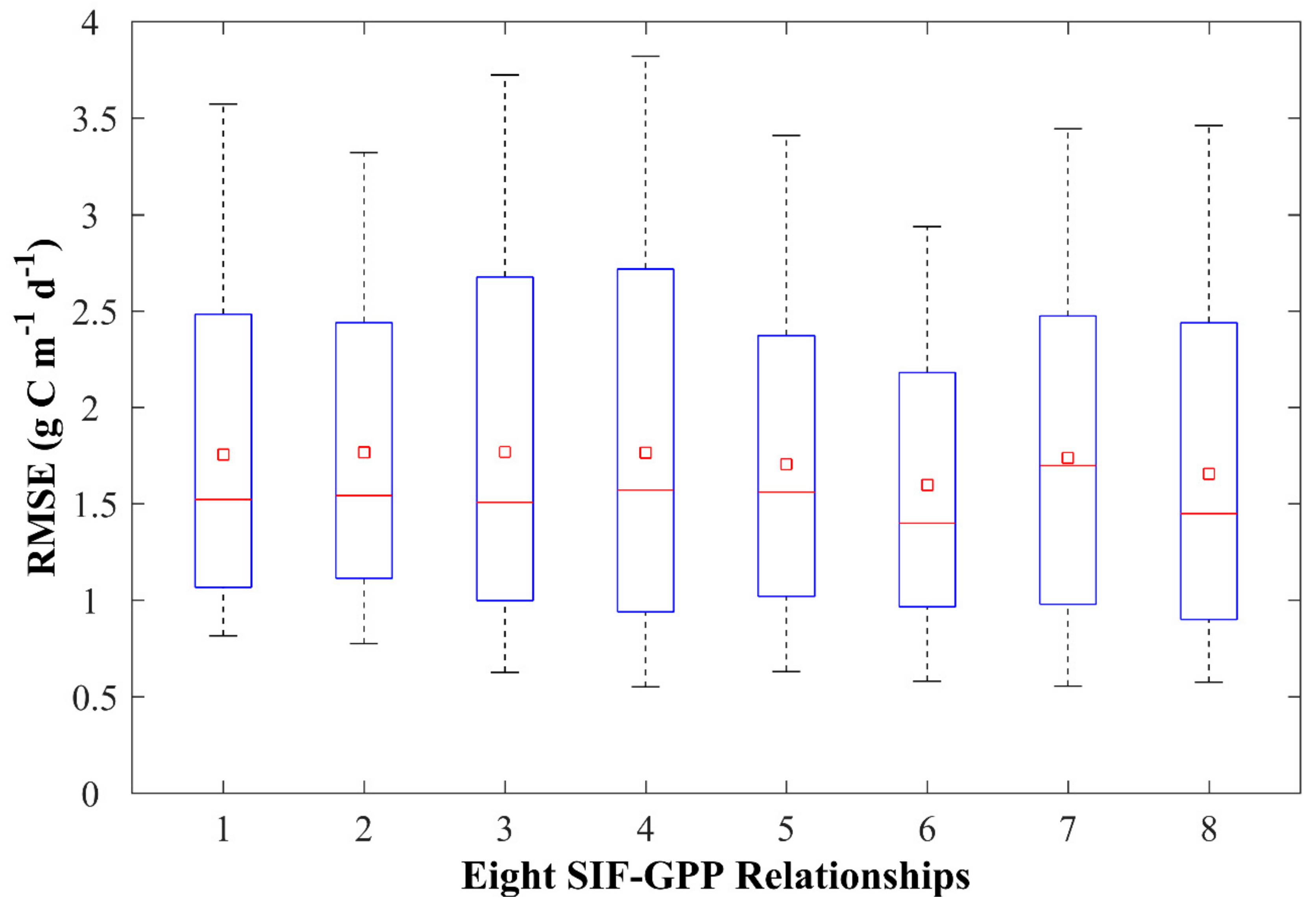
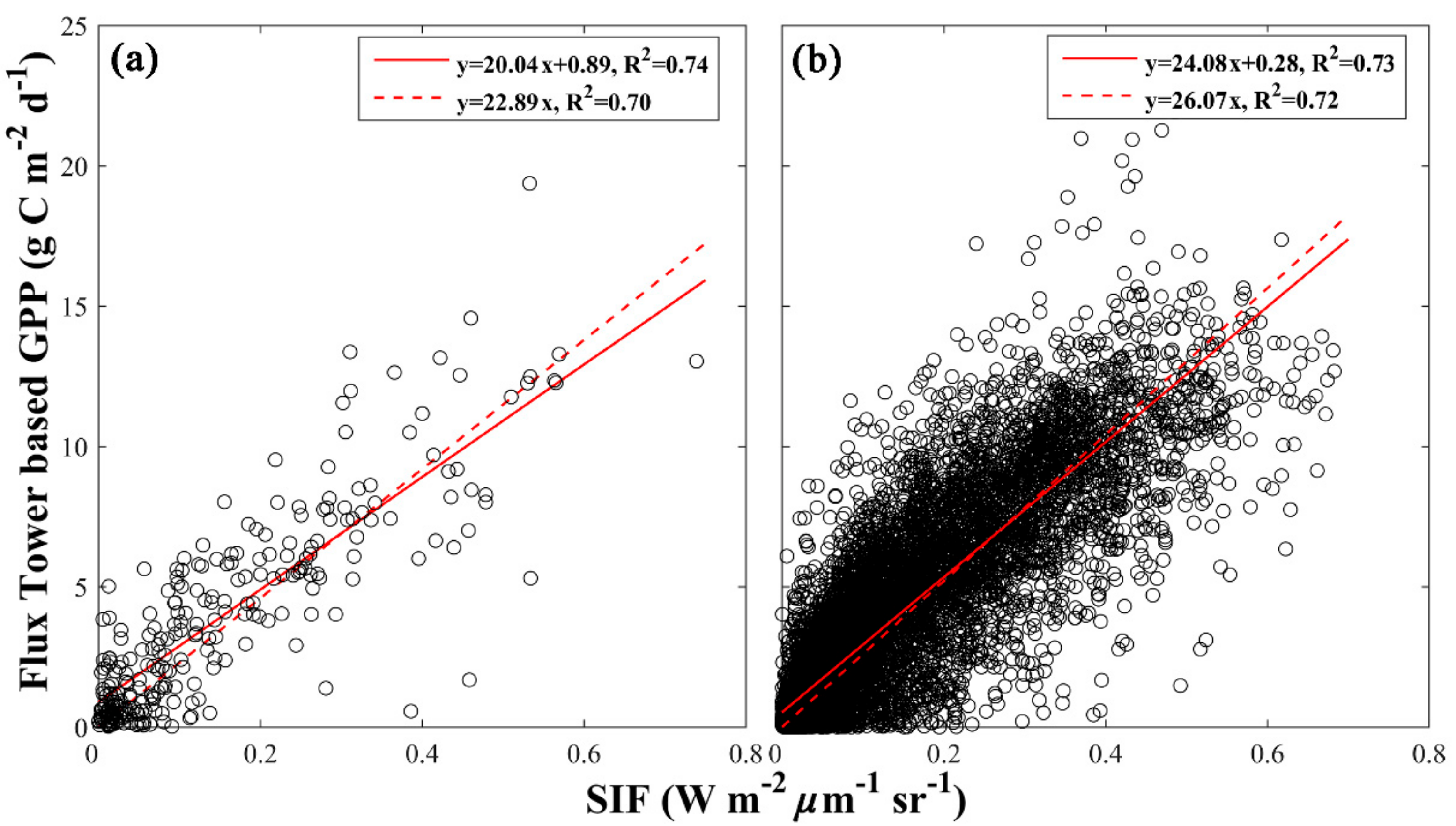
3.1. Evaluating Different SIF-GPP Relationships

We estimated GPP globally from SIF based on the fine-resolution GOSIF product [31] and a total of eight SIF-GPP relationships that we established (both universal and biome-specific; both non-zero and zero intercept; both site and grid cell level). The scatterplots of the SIF-GPP relationships at both site and grid cell level are shown in Figure 1, and the statistical measures (slope, intercept, and R2) are provided in Table 1. The strength of the SIF-GPP relationship found at the site level (R2 = 0.70–0.74, p < 0.001) was comparable to that at the grid cell level (R2 = 0.72–0.73, p < 0.001). The slope of the grid cell level relationships for about half of the biomes (e.g., evergreen needleleaf forests, evergreen broadleaf forests, open shrublands) was higher than that of the site-level relationships, possibly due to the heterogeneity within the 0.05° grid cells in which some EC sites are located or the slight underestimation of our gridded SIF (GOSIF) for these biomes (Table 1).
The universal SIF-GPP relationship at the ecosystem level (i.e., site level) estimated GPP fairly well at the site level, and other SIF-GPP relationships also estimated GPP fairly well (Figure 2). The performance was similar among the eight relationships with site-mean RMSE ranging from 1.60 to 1.77 g C m−2 d−1. The site-level relationships (i.e., the relationships based on SIF from OCO-2 soundings and tower GPP from 64 EC sites; boxplots 1-4 in Figure 2) had almost identical performance, suggesting that the SIF-based approach was relatively insensitive to the specific forms of the SIF-GPP relationship (universal or biome-specific, with or without intercept). The performance of the grid cell level relationships (i.e., the relationships derived based on 0.05° SIF and tower GPP; boxplots 5-8 in Figure 2) was slightly affected by the use of non-zero or zero intercept. At the grid cell level, the biome-specific relationships were slightly better than the universal ones.

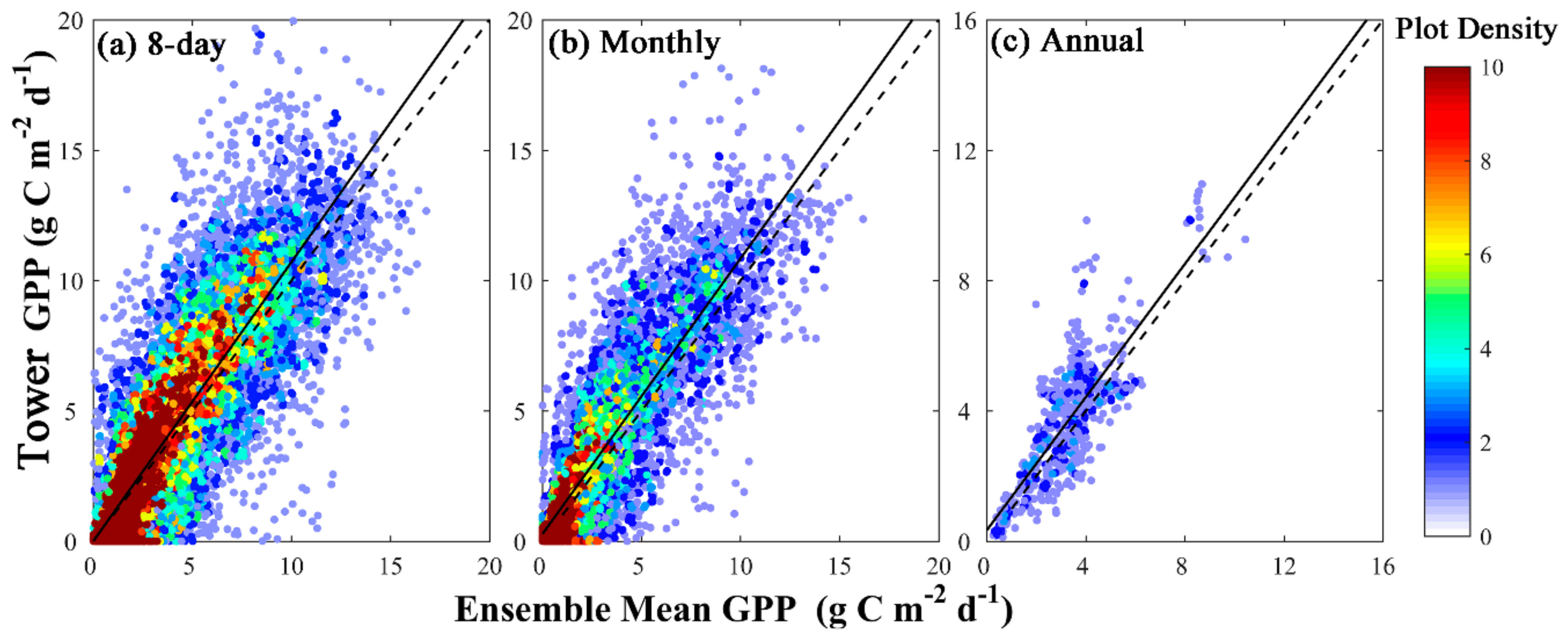
3.2. Validating Gridded GPP Estimates Derived from GOSIF

We estimated GPP from 2000–2017 at 8-day intervals and on a 0.05° × 0.05° grid across the globe based on the GOSIF product and the eight SIF-GPP relationships separately. The universal SIF-GPP relationship developed at the site level estimated GPP fairly well (R2 = 0.72, RMSE = 2.04 g C m−2 d−1). The biome-specific relationships and other forms of relationships also estimated GPP fairly well. These different SIF-GPP relationships led to an ensemble GPP product, referred to as GOSIF GPP. For each grid cell and each interval, we calculated the ensemble mean GPP and used the ensemble standard deviation as a measure of uncertainty in GPP. Our ensemble mean GPP derived from eight SIF-GPP relationships was generally highly correlated with the flux tower GPP for 91 open-access EC sites from FLUXNET 2015 Tier-1 across the globe at the 8-day timestep (R2 = 0.74, RMSE = 1.92 g C m−2 d−1; Figure 3). The correlations at the 8-day timescale were consistently strong among biomes with R2 ranging from 0.51 to 0.85. GPP was slightly underestimated for evergreen needleleaf forests, open shrublands, and grasslands, and was slightly overestimated for evergreen broadleaf forests. We provided the distribution map of R2 and RMSE for all flux sites in Figure S1. We also aggregated our 8-day GPP estimates to monthly and annual scales, and the aggregated GPP also agreed with flux tower GPP fairly well at both monthly (R2 = 0.75, RMSE = 1.90 g C m−2 d−1) and annual scales (R2 = 0.65, RMSE = 1.21 g C m−2 d−1). The R2 and RMSE between estimated GPP and tower GPP for each biome at different scales are summarized in Table 2. The ensemble mean annual GPP in 2010 was strongly correlated to EC-MOD GPP (R2 = 0.87, RMSE = 0.91 g C m−2 d−1). The relationship was strong for most biomes and moderately strong for certain biomes with lower spatial variability (Figure S2).
The estimated GPP could capture the interannual variability of tower GPP at the site level to some extent (R2 = 0.77, p < 0.001; Figure 4a). Our GPP estimates also characterized the anomalies of annual GPP in each year (R2 = 0.62, p<0.001; Figure 4b). The consistency in interannual variability between estimated and tower GPP was generally strong for non-forests sites and generally weak for forests sites (Figure S3). Both figures showed that GOSIF GPP underestimated the interannual variability of tower GPP to a certain degree.
The spatial and seasonal variations of GPP based on the universal SIF-GPP relationship across the globe are illustrated in Figure S4. The GOSIF GPP had relatively strong seasonal cycles in the Northern Hemisphere and smaller seasonal fluctuations in the Southern Hemisphere. The prominently high GPP values were found in some agricultural regions in summer (e.g., the U.S. Corn Belt region, northeastern China, and central Europe).
For comparison purposes, we also used the universal SIF-GPP relationship (site-level, with slope; Table 1) to generate coarse-resolution (1°) GPP estimates from the coarse-resolution SIF estimates (1°, monthly) directly aggregated from discrete OCO-2 SIF soundings. We then compared the spatial patterns of our finer-resolution GOSIF GPP maps with those of the coarse-resolution GPP in three selected geographical regions (United States, Australia, and East Asia) (Figure 5). GOSIF GPP with finer resolutions fully captured the spatial patterns and seasonal cycles present in the coarse-resolution (1°) data. For example, in United States and East Asia (Figure 5a,b), GPP exhibited the highest values in July, intermediate values in April and October, and the lowest values in January; in Australia (Figure 5c), the majority of grid cells are dominated by drylands and exhibited low GPP values throughout the year, while higher GPP in eastern and southeastern Australia in the wet season was also captured. The coarse-resolution GPP estimates had tremendous data gaps, while our ensemble GPP had globally continuous coverage and much finer spatial details. This finer-resolution GOSIF GPP dataset provides a valuable opportunity to examine terrestrial photosynthesis at various scales from ecosystem to the globe.

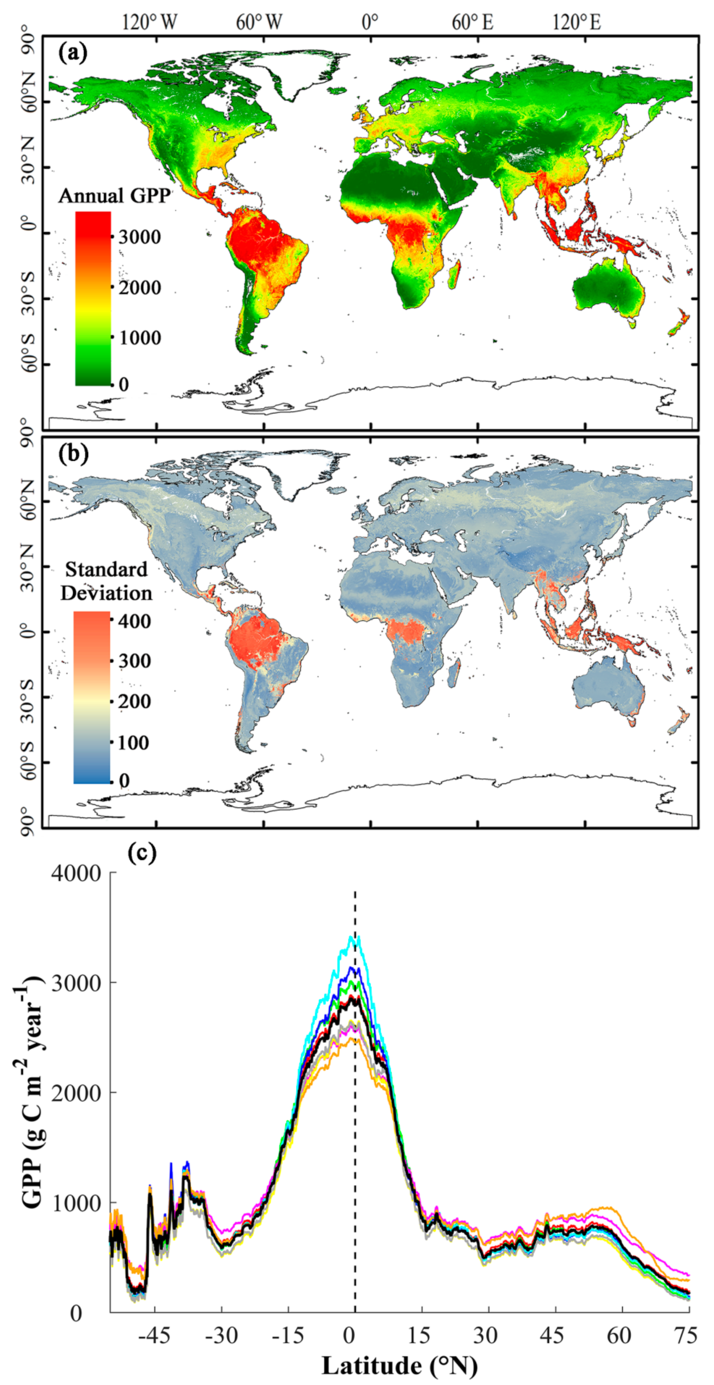
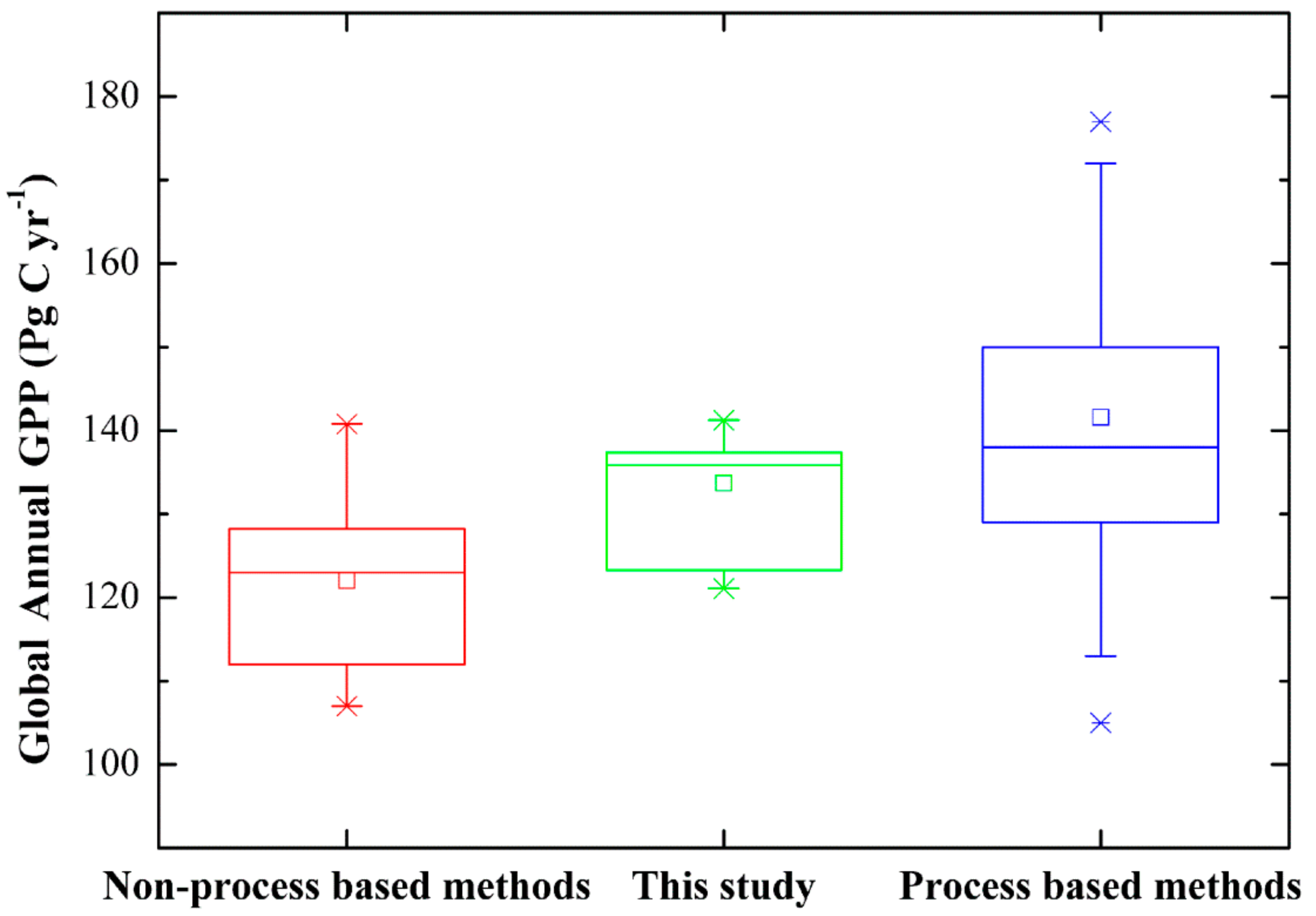
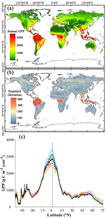
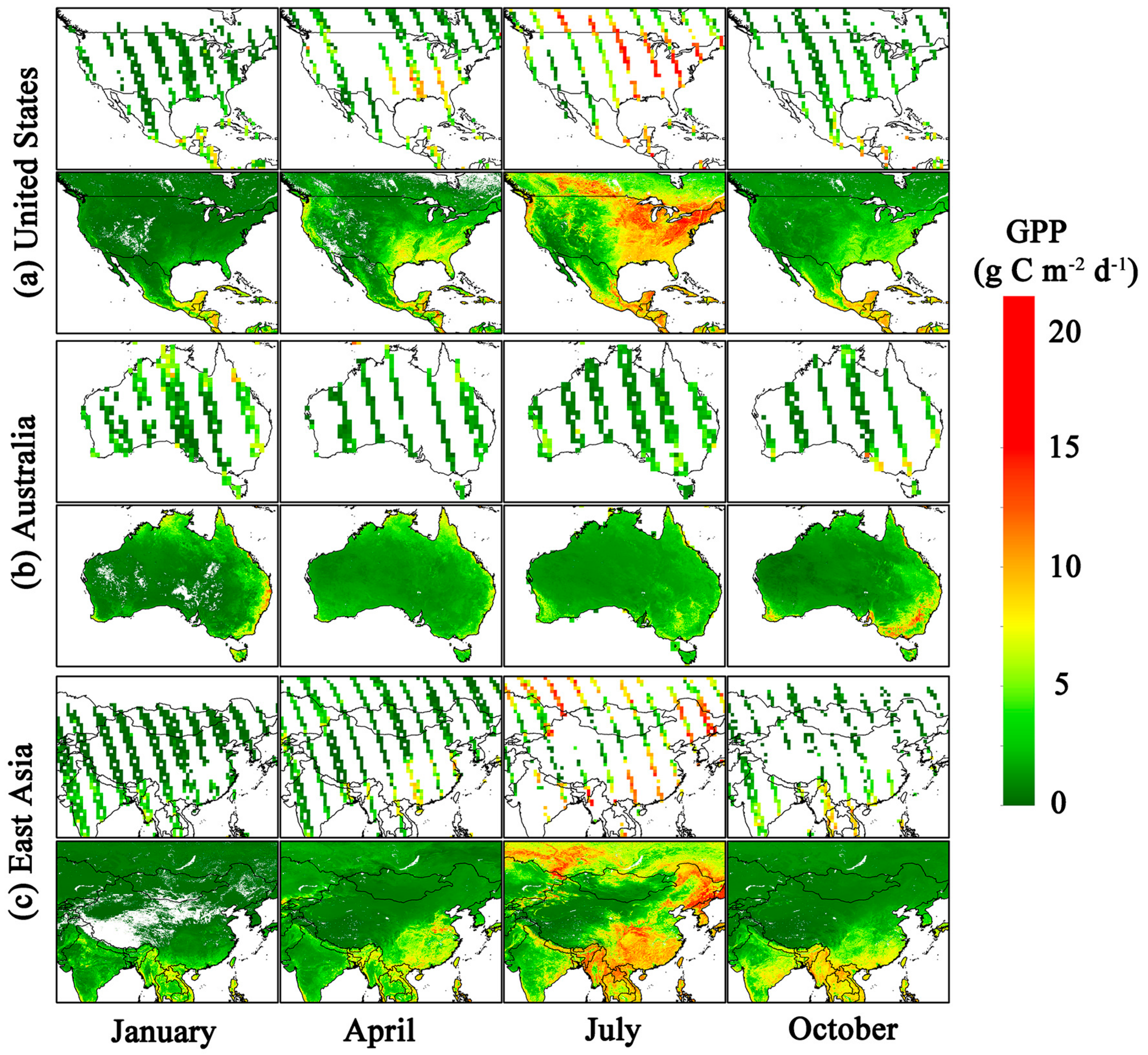
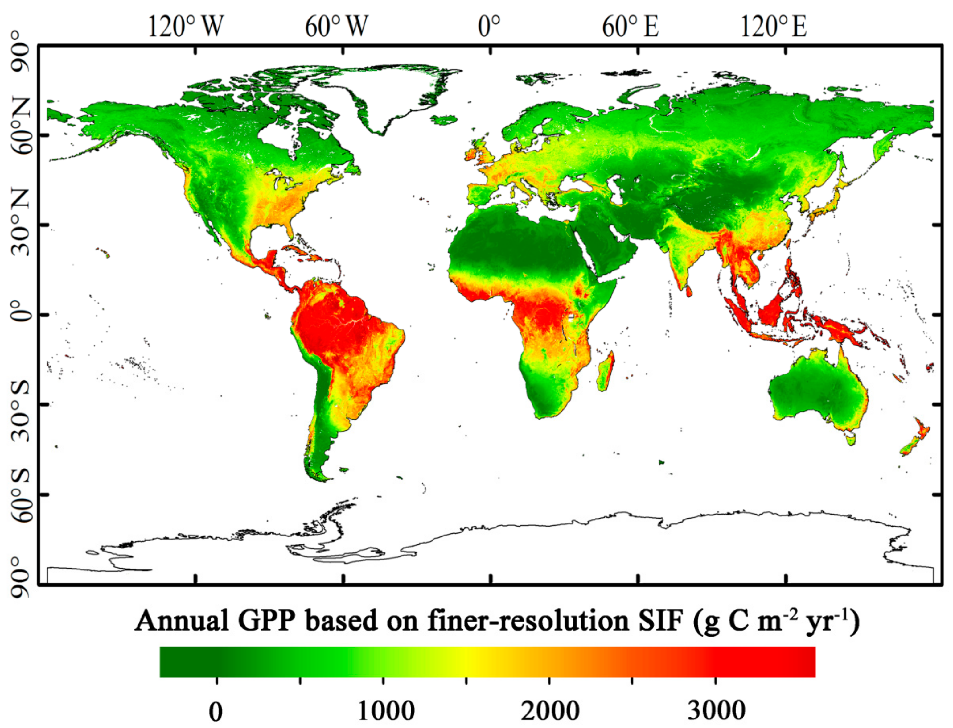
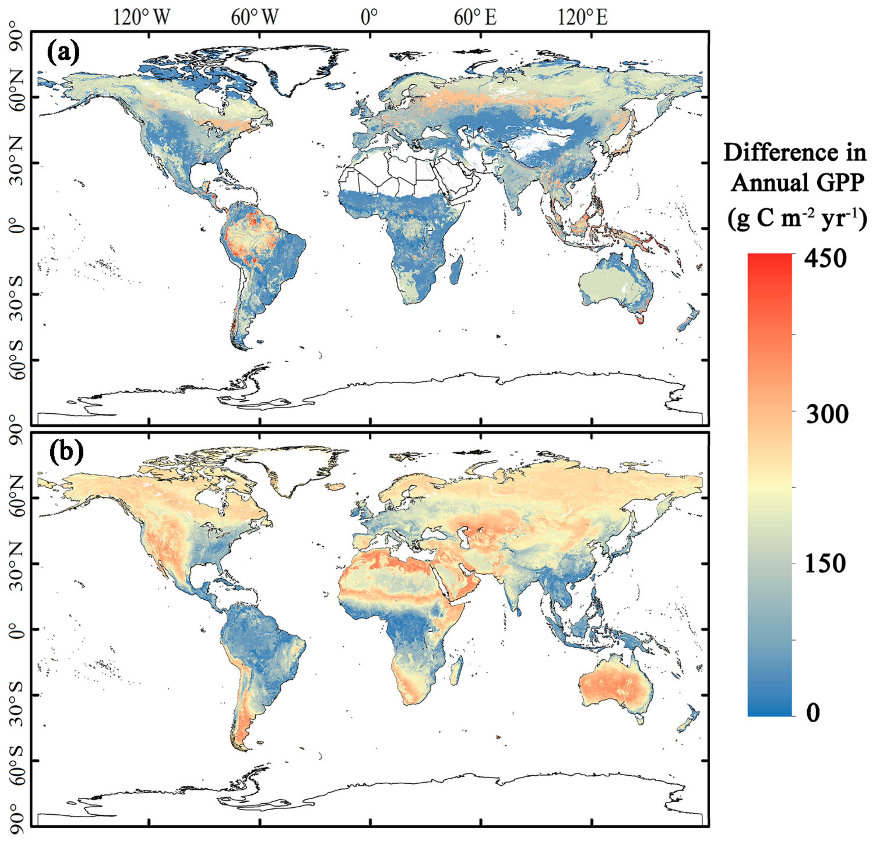
3.3. Magnitude and Patterns of Annual GPP

The annual GPP based on the universal SIF-GPP relationship (site-level, with intercept) exhibited expected magnitude and spatial pattern across the globe (Figure 6). The highest values of annual GPP were observed in the tropical regions (2500–3500 g C m−2 yr−1), intermediate values in the eastern United States and southern Asia (1000–2000 g C m−2 yr−1), and the lowest values in the sparsely vegetated regions (0–500 g C m−2 yr−1).
We then examined how the universal versus biome-specific nature of the SIF-GPP relationship affected the GPP estimates derived from SIF. Figure 7a shows that the difference in annual GPP based on a universal versus biome-specific relationship was generally small across the globe. Relatively large differences were only observed in some highly productive tropical regions and some high-latitude regions. We also examined how the use of the non-zero intercept versus zero intercept influenced GPP estimates for the universal SIF-GPP relationship (site-level). Compared to the use of the zero-intercept, the use of a non-zero intercept resulted in higher annual GPP in regions with low productivity (Figure 7b), indicating that the magnitude of GPP estimates could be significantly influenced by whether the intercept is forced to be zero.
To account for the uncertainty in GPP estimates resulting from different forms of SIF-GPP relationships (i.e., universal and biome-specific, with and without intercept), we used the eight SIF-GPP relationships to map GPP globally from GOSIF. The magnitude and spatial pattern of mean annual GPP calculated from the ensemble GPP estimates (Figure 8a) were very similar to those based on the site-level, universal SIF-GPP relationship (Figure 6). The standard deviation of annual GPP (Figure 8b) showed that the eight SIF-GPP relationships led to the largest variability in GPP in the tropical regions with high productivity. This discrepancy of annual GPP among the ensemble estimates exhibited clear latitudinal patterns (Figure 8c). The tropics (−15 °S to 15°N) had the largest variability in annual GPP among the eight sets of estimates. The maximum GPP, which shows the seasonal peak of vegetation photosynthesis, captured the typical crop planting areas worldwide (Figure S5). The latitudinal pattern of the maximum GPP had two other peaks centered around −35° S and 60 °N (Figure S5c) compared with that of annual GPP (Figure 8c).
The ensemble global mean annual GPP estimated by our method is 135.5 ± 8.8 Pg C yr−1 for the period from 2001 to 2017 (Figure 9). Although the eight SIF-GPP relationships overall had similar performance in estimating GPP at the grid cell level (Figure 2), the difference was magnified when GPP was aggregated from the grid cell level to the globe. For the two different possible forms (universal and biome-specific; non-zero and zero intercept) of the SIF-GPP relationship, the global annual GPP was more affected by whether the relationship was forced to pass through the origin, which could lead to a difference up to 9.4 Pg C yr−1 (grid cell level relationships) or 19.1 Pg C yr−1 (site-level relationships). These findings were consistent with the annual GPP difference in Figure 7.
There has been tremendous interest in quantifying global GPP, and the estimates from the literature are summarized in Table S2 and illustrated in Figure 9. There was substantial spread in current global annual GPP estimates. In general, the global GPP estimated by non-process based methods had smaller magnitudes and narrower ranges, while the process-based models generally showed higher global GPP and larger spread across different models. Our ensemble mean is higher than the mean estimate from non-process based methods and slightly lower than that from process-based models (Figure 9).

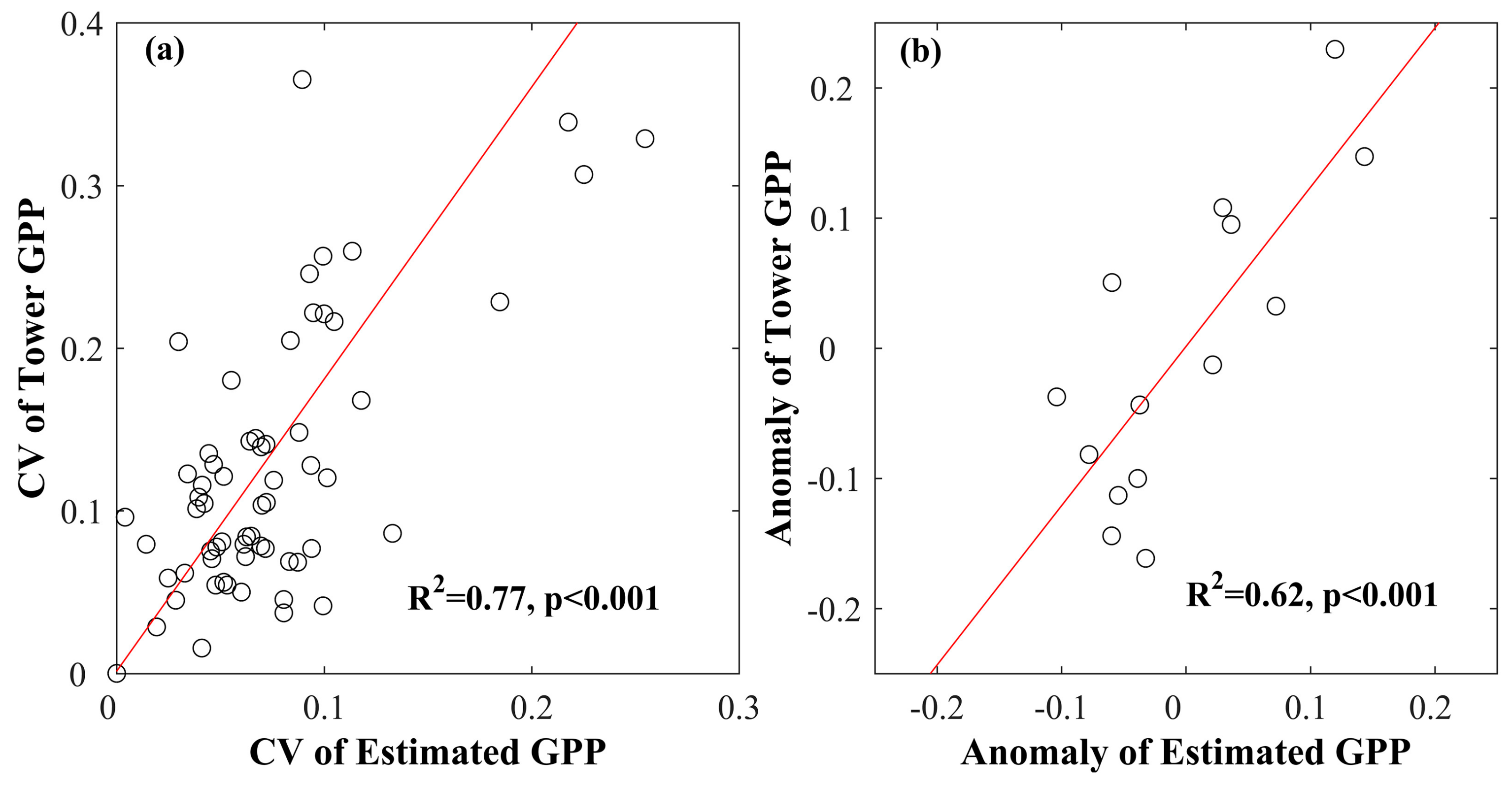
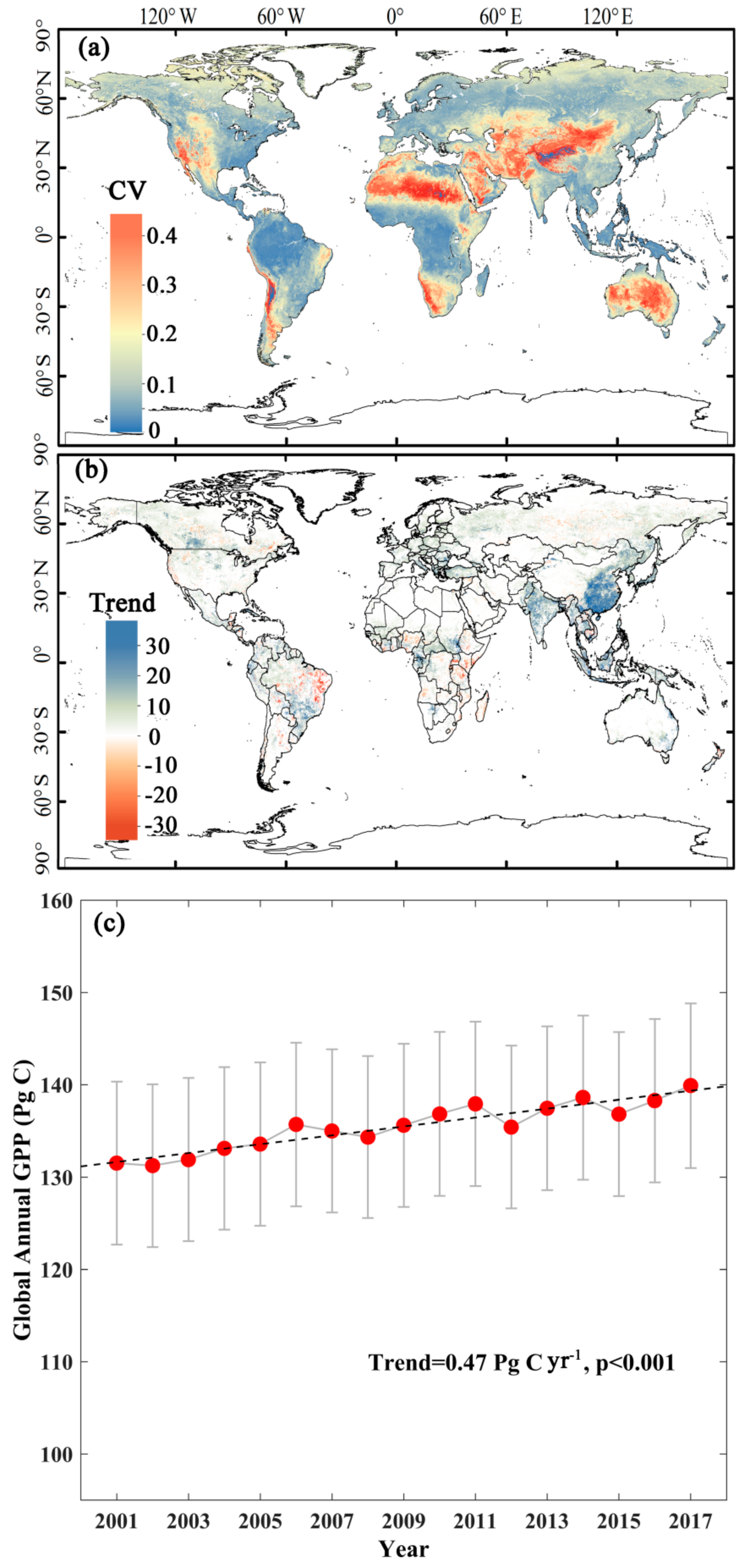
3.4. Interannual Variability and Trend of Annual GPP

We examined the interannual variability in GPP using the coefficient of variation (CV) (Figure 10a). Large CV values were generally observed in arid or semi-arid areas such as Australia, central Asia, and the Sahara Desert. During the period from 2001 to 2017, only about 31.4% of the vegetated land area showed a significant trend in GPP (p < 0.05, Figure 10b). The areas with a positive trend were more widespread than the areas with negative trends. The mean global GPP significantly increased during the 17-year period (0.47 Pg C per year, p < 0.001) (Figure 10c).

4. Discussion

The advent of SIF measured from space and the elucidation of the relationship between SIF and GPP constitute a milestone in remote sensing of the terrestrial carbon cycle [41]. We mapped GPP globally with fine spatial (0.05°) and temporal (8-day) resolutions from our recently produced GOSIF data (a new global, fine-resolution SIF product based on OCO-2 SIF) [31] and the SIF-GPP relationships that we established. Many studies have shown the strong potential of SIF in estimating GPP through analytical models, field measurements, or satellite data in recent years 1 [11,16,17,26,32,33,42,43]. Some earlier studies showed strong SIF-GPP relationships based on coarse-resolution SIF (e.g., GOME-2 or GOSAT) and gridded GPP products [10,21,22,44]. Several more recent studies found strong ecosystem-level relationships based on OCO-2 SIF and tower GPP [17,26,36]. Satellite-based SIF has also been recently used to constrain carbon-related model parameters [22,45,46] or identify regions of high productivity crops [47]. However, direct estimation of GPP from satellite SIF at the regional or global scale is challenging mainly due to the following three reasons. First, finer spatial resolution (e.g., several to tens of square kilometers) gridded SIF observations are currently not available. Second, although OCO-2 SIF with much smaller ground size provides a valuable opportunity to direclty link satellite-measured SIF with flux tower GPP to examine the SIF-GPP relationship [8,16,17,25,26], generating finer-resolution GPP is hindered by the sparse global coverage of OCO-2 data. Third, the relationship between GPP and SIF for all the main biome types based on finer-resolution SIF data and high-quality flux tower GPP (rather than gridded GPP products) has not been established until very recently [17].
We mapped GPP globally based on the fine-resolution, OCO-2-based SIF product (GOSIF) that we recently developed [31] and SIF-GPP relationships that we established. We used both a universal SIF-GPP relationship across a wide variety of biomes and biome-specific relationships that we previously established [17]. We also examined how the use of the intercept versus zero-intercept and the spatial scale used to develop the SIF-GPP relationships (site level versus grid cell level) influenced GPP estimates. To account for the uncertainty in the resulting GPP estimates, we produced eight global GPP products based on eight established SIF-GPP relationships consisting of both site and grid cell level relationships and different forms of the SIF-GPP relationship (both universal and biome-specific, both zero and non-zero intercept). This analysis provides insight into how well GPP can be estimated based on the SIF-GPP relationship by validating the resulting GPP estimates against tower GPP from 91 EC flux sites, and also reveals how the uncertainty in GPP estimates propagates to the global scale. The SIF-GPP relationships with different forms had negligible influence on the estimated 8-day GPP at the grid cell level (or at the scale of a flux tower), while it could lead to a difference up to 400 g C m−2 year−1 in predicted annual GPP at the grid cell level or up to ~20 Pg C yr−1 in global annual GPP. The relatively large discrepancy in global annual GPP among products based on the different SIF-GPP relationships was mainly caused by the overestimation based on the SIF-GPP relationships with a non-zero intercept, which lead to a widespread increase in annual GPP for regions with lower productivity. For example, the intercept of 0.89 g C m−2 day−1/W m−2μm−1 sr−1 for the site-level relationship gave rise to a difference of 19. 1 Pg C yr−1 in global annual GPP compared to the site-level relationship without an intercept. By contrast, applying a universal versus biome-specific relationship resulted in a small difference in global annual GPP. The biases in both OCO-2 SIF and GPP data could alter the SIF-GPP relationships. The ensemble mean GPP from our eight sets of GPP estimates could reduce the uncertainty to a certain extent. The uncertainty of the GPP estimates could also result from the uncertainty in our gridded SIF estimates. The prediction of SIF was affected by several factors, such as explanatory variables used in the predictive model, training sample size or uncertainty of the gridded input data products [31], and the errors associated with these factors could be propagated to the GPP estimates. For the GPP estimates based on the grid cell level relationships between SIF and GPP, the scale mismatch between the tower footprint and the 0.05° grid cell could affect the developed SIF-GPP relationships and consequently introduce uncertainty to the GPP estimates. The ensemble GPP estimates resulting from the different SIF-GPP relationships can partly account for these uncertainties, and the ensemble mean is likely more suitable for examining GPP globally than a single GPP product.
Capturing the interannual variability well is still a grand challenge for both non-process and process-based methods in carbon cycle studies. Our approach also underestimated the interannual variability in GPP. The establishment of our SIF-GPP relationships is based on the short record of OCO-2 SIF which is likely to be insufficient to account for the interannual variability of GPP. The availability of a longer fine-resolution SIF record in the future is expected to improve GPP estimates and better capture the interannual variability of GPP. In addition, we did not separate C3 and C4 for croplands and grasslands due to a limited number of samples at the site level. Several previous studies found that the GPP-SIF relationship had a higher slope for C4 ecosystems than for C3 ecosystems [17,25,48]. In our site-based analysis, the observed much higher slope of C4 species was mainly contributed by one corn site [17]. Future work should explore whether and how the differentiation of C3 and C4 ecosystems could influence the accuracy of the resulting GPP estimates for croplands and grasslands.
The overall spatial pattern of annual GPP found in our study was consistent with GPP estimates based on satellite-based production efficiency models [49], process-based models [50,51], and data-driven methods [5,52]. The pattern of maximum daily GPP throughout a year is generally similar to that of the maximum daily productivity based on GPP estimates [53] or directly inferred from coarse-resolution SIF data [33,54]. Our estimate of global annual GPP (135.5 ± 8.8 Pg C yr−1) is between the 75th percentile and 95th percentile of the estimates from non-process based methods and higher than the estimate (~110 Pg C yr−1) from the MODIS GPP product [49] and the estimates from data-driven methods (119 - 123 Pg C yr−1) [5,52]. The estimates of global GPP from process-based models varied from 98 to 177 Pg C yr−1 [6,7], and our estimate is slightly lower that the 50th percentile of these estimates. A variety of factors could lead to large biases in global GPP estimates, such as imperfect model structures, parameter uncertainty, and the errors of input variables (e.g., climate forcing, land cover map) [55]. Our global GPP estimate is between the mean estimate of the non-process based methods and process-based models.
Our GOSIF GPP product is useful for benchmarking state-of-the-art terrestrial biosphere/Earth system models. These models exhibit substantial uncertainty in GPP estimates due to various sources of uncertainty. It is challenging to evaluate these models partly because of the lack of reference data at regional to global scales. Our SIF-derived GPP product provides a new and independent dataset that can be used to benchmark terrestrial biosphere models and ESMs. The benchmarking exercise will help determine how well the state-of-the-art models can simulate the magnitude, patterns, and interannual variability of terrestrial photosynthesis and shed light on directions for future model improvement.
Our study demonstrated the tremendous capability of SIF observed from space in mapping terrestrial GPP globally, and is also enlightening for future efforts using SIF measured from space. This advance leads to a new, independent approach in measuring terrestrial photosynthesis compared to traditional methods (e.g., process-based models, light use efficiency models, data-driven methods). The process-based models generally have complex structure, and require a variety of input data that could have significant uncertainty [55]. The data-driven methods also rely on a large number of explanatory variables to estimate GPP [38,52]. Even the light use efficiency (LUE) models [56,57] with a simple model structure (e.g., the MODIS GPP model) have several different input variables such as land cover, the fraction of PAR absorbed by vegetation canopies (fPAR), PAR, and two environmental scalars used to characterize temperature and water stresses and also include multiple models parameters (e.g., maximum LUE, optimum temperature). The use of these ancillary data such as gridded land cover and meteorological data can lead to significant uncertainty to the resulting GPP estimates [58]. Our novel, SIF-based approach can lead to more accurate GPP estimates at regional to global scales by avoiding uncertainties from other data (e.g., climate, soil properties). Although the gridded SIF data (GOSIF) were generated based on OCO-2 SIF along with EVI, temperature, PAR, and VPD, these ancillary data layers were simply used to help generate spatially continuous, fine-resolution SIF estimates from discrete OCO-2 soundings. With the availability of spatially continuous, high-quality SIF measurements (e.g., the ongoing TROPOspheric Monitoring Instrument or TROPOMI, 0.1° resolution; the upcoming FLuorescence EXplorer or FLEX, 300 m resolution), our SIF-based approach will be able to generate more accurate GPP estimates regionally and globally by avoiding the uncertainty associated with input data (e.g., climate forcing). The use of the universal SIF-GPP relationship across a variety of biomes [17] can also avoid the uncertainty associated with land cover maps. Our novel method also has lower computational demand than other approaches, and can potentially provide more accurate, near real-time estimates of terrestrial photosynthesis globally from space.

5. Conclusions

The OCO-2 provides SIF soundings with a small footprint (1.3 km × 2.25 km), offering a valuable opportunity to establish a more robust relationship between SIF measured from space and GPP data from flux towers. However, generating finer-resolution global GPP estimates from OCO-2 SIF was hindered by OCO-2’s sparse coverage and reliable SIF-GPP relationship. In this study, we developed a continuous gridded global GPP data product (GOSIF GPP) for the period 2000–2017 from the recently-generated global, OCO-2 based SIF product (GOSIF) with fine-resolution (i.e., 0.05°, 8-day) using a set of SIF-GPP relationships. Our results showed that all of the eight SIF-GPP relationships could estimate GPP fairly well, and the ensemble mean 8-day GPP based on the eight SIF-GPP relationships was generally highly correlated with flux tower GPP for 91 FLUXNET sites across the globe (R2=0.74, RMSE = 1.92 g C m−2 d−1). The ensemble mean GPP showed reasonable spatial and seasonal variations across the globe, and fully captured both spatial and seasonal patterns present in the coarse-resolution (1°) GPP estimates based on coarse-resolution SIF data directly aggregated from discrete OCO-2 soundings. Our results showed that the difference in annual GPP based on a universal versus biome-specific relationship was generally small across the globe, while the magnitude of the annual GPP could be significantly influenced by whether the intercept was forced to be zero. Our global GPP estimate (135.5 ± 8.8 Pg C yr−1) is between the median estimate of non-process based methods and the median estimate of process-based models. Significant interannual variability in GPP was observed in many parts of the globe. Annual GPP also exhibited increasing trends in many areas, particularly in the Northern Hemisphere. The different SIF-GPP relationships could lead to significant differences in annual GPP, particularly in the tropics. The further elucidation of the SIF-GPP relationship is expected to reduce the uncertainty of the resulting GPP estimates.
Our SIF-based method is a new and independent approach for estimating terrestrial photosynthesis regionally and globally. With the availability of high-quality, gridded SIF observations from space (e.g., TROPOMI, FLEX), this novel approach can lead to gridded GPP estimates solely based on SIF observations and does not rely on any input data (e.g., climate data, soil properties). The use of a universal SIF-GPP relationship can also avoid the uncertainty associated with land cover maps. Our approach can potentially lead to more accurate, near real-time GPP estimates regionally and globally. Our novel, fine-resolution GPP product (GOSIF GPP), freely available at our data repository (http://globalecology.unh.edu), will be valuable for studying ecosystem functioning and carbon cycling, monitoring agricultural production, informing ecosystem management, and benchmarking state-of-the-art terrestrial biosphere/Earth system models (ESMs).

Supplementary Materials

The following are available online at https://0-www-mdpi-com.brum.beds.ac.uk/2072-4292/11/21/2563/s1, Figure S1: Spatial patterns of R2 and RMSE between our ensemble mean 8-day GPP and flux tower GPP for each site, Figure S2: Validation of ensemble mean annual GPP against EC-MOD GPP in 2010, Figure S3. Validation of the interannual variability of GOSIF GPP for each site, Figure S4: Spatial patterns of our global ensemble mean GPP from January through December in 2016, Figure S5: Spatial patterns and magnitude of global maximum GPP, Table S1: FLUXNET Tier-1 sites used for validating the gridded GPP estimates in this study, Table S2: Estimates of annual global GPP based on both non-process methods and process-based models.

Author Contributions

J.X. and X.L. designed the research. X.L. processed the data. X.L. and J.X. analyzed the data and wrote the paper.

Funding

This study was financially supported by the National Aeronautics and Space Administration (NASA)’s Climate Indicators and Data Products for Future National Climate Assessments (Grant number: NNX16AG61G) and Carbon Cycle Science Program (Grant number: NNX14AJ18G).

Acknowledgments

The eddy covariance data were collected, processed, and shared by the FLUXNET community. The processing and harmonization of the FLUXNET data were conducted by the European Fluxes Database Cluster, the AmeriFlux Management Project, and the Fluxdata project of FLUXNET.

Conflicts of Interest

The authors declare no conflict of interest.

References

  1. Le Quéré, C.; Moriarty, R.; Andrew, R.M.; Canadell, J.G.; Sitch, S.; Korsbakken, J.I.; Friedlingstein, P.; Peters, G.P.; Andres, R.J.; Houghton, R.A.; et al. Global carbon budget 2015. Earth Syst. Scie. Data 2015, 7, 349–396. [Google Scholar]
  2. Amiro, B.; Barr, A.; Barr, J.; Black, T.A.; Bracho, R.; Brown, M.; Chen, J.; Clark, K.; Davis, K.; Dore, S.; et al. Ecosystem carbon dioxide fluxes after disturbance in forests of North America. J. Geophys. Res. Biogeosci. 2010, 115. [Google Scholar] [CrossRef]
  3. Xiao, J.; Zhuang, Q.; Liang, E.; Shao, X.; McGuire, A.D.; Moody, A.; Kicklighter, D.W.; Melillo, J.M. Twentieth-century droughts and their impacts on terrestrial carbon cycling in China. Earth Interact. 2009, 13, 1–31. [Google Scholar] [CrossRef]
  4. Ito, A.; Saigusa, N.; Murayama, S.; Yamamoto, S. Modeling of gross and net carbon dioxide exchange over a cool-temperate deciduous broad-leaved forest in Japan: analysis of seasonal and interannual change. Agric. For. Meteorol. 2005, 134, 122–134. [Google Scholar] [CrossRef]
  5. Beer, C.; Reichstein, M.; Tomelleri, E.; Ciais, P.; Jung, M.; Carvalhais, N.; Rödenbeck, C.; Arain, M.A.; Baldocchi, D.; Bondeau, A.; et al. Terrestrial gross carbon dioxide uptake: global distribution and covariation with climate. Science 2010, 329, 834–838. [Google Scholar] [CrossRef]
  6. Anav, A.; Friedlingstein, P.; Kidston, M.; Bopp, L.; Ciais, P.; Cox, P.; Jones, C.; Jung, M.; Myneni, R.; Zhu, Z.; et al. Evaluating the land and ocean components of the global carbon cycle in the CMIP5 Earth System Models. J. Clim. 2013, 26, 6801–6843. [Google Scholar] [CrossRef]
  7. Ito, A.; Nishina, K.; Reyer, C.P.; François, L.; Henrot, A.-J.; Munhoven, G.; Jacquemin, I.; Tian, H.; Yang, J.; Morfopoulos, C.; et al. Photosynthetic productivity and its efficiencies in ISIMIP2a biome models: benchmarking for impact assessment studies. Environ. Res. Lett. 2017, 12, 085001. [Google Scholar] [CrossRef]
  8. Frankenberg, C.; O’Dell, C.; Berry, J.; Guanter, L.; Joiner, J.; Köhler, P.; Pollock, R.; Taylor, T.E. Prospects for chlorophyll fluorescence remote sensing from the Orbiting Carbon Observatory-2. Remote Sens. Environ. 2014, 147, 1–12. [Google Scholar] [CrossRef] [Green Version]
  9. Joiner, J.; Guanter, L.; Lindstrot, R.; Voigt, M.; Vasilkov, A.; Middleton, E.; Huemmrich, K.; Yoshida, Y.; Frankenberg, C. Global monitoring of terrestrial chlorophyll fluorescence from moderate spectral resolution near-infrared satellite measurements: Methodology, simulations, and application to GOME-2. Atmos. Meas. Tech. 2013, 6, 2803–2823. [Google Scholar] [CrossRef]
  10. Guanter, L.; Frankenberg, C.; Dudhia, A.; Lewis, P.E.; Gómez-Dans, J.; Kuze, A.; Suto, H.; Grainger, R.G. Retrieval and global assessment of terrestrial chlorophyll fluorescence from GOSAT space measurements. Remote Sens. Environ. 2012, 121, 236–251. [Google Scholar] [CrossRef]
  11. Frankenberg, C.; Fisher, J.B.; Worden, J.; Badgley, G.; Saatchi, S.S.; Lee, J.E.; Toon, G.C.; Butz, A.; Jung, M.; Yokota, T.; et al. New global observations of the terrestrial carbon cycle from GOSAT: Patterns of plant fluorescence with gross primary productivity. Geophys. Res. Lett. 2011, 38. [Google Scholar] [CrossRef] [Green Version]
  12. Ryu, Y.; Berry, J.A.; Baldocchi, D.D. What is global photosynthesis? History, uncertainties and opportunities. Remote Sens. Environ. 2019, 223, 95–114. [Google Scholar] [CrossRef]
  13. Köhler, P.; Frankenberg, C.; Magney, T.S.; Guanter, L.; Joiner, J.; Landgraf, J. Global Retrievals of Solar-Induced Chlorophyll Fluorescence With TROPOMI: First Results and Intersensor Comparison to OCO-2. Geophys. Res. Lett. 2018, 45, 10456–10463. [Google Scholar]
  14. Gu, L.; Han, J.; Wood, J.D.; Chang, C.Y.Y.; Sun, Y. Sun-induced Chl fluorescence and its importance for biophysical modeling of photosynthesis based on light reactions. New Phytol. 2019, 1. [Google Scholar] [CrossRef] [PubMed]
  15. Baker, N.R. Chlorophyll fluorescence: a probe of photosynthesis in vivo. Annu. Rev. Plant Biol. 2008, 59, 89–113. [Google Scholar] [CrossRef]
  16. Li, X.; Xiao, J.; He, B. Chlorophyll fluorescence observed by OCO-2 is strongly related to gross primary productivity estimated from flux towers in temperate forests. Remote Sens. Environ. 2018, 204, 659–671. [Google Scholar] [CrossRef]
  17. Li, X.; Xiao, J.; He, B.; Arain, M.A.; Beringer, J.; Desai, A.R.; Emmel, C.; Hollinger, D.Y.; Krasnova, A.; Noe, S.M.; et al. Solar-induced chlorophyll fluorescence is strongly correlated with terrestrial photosynthesis for a wide variety of biomes: First global analysis based on OCO-2 and flux tower observations. Glob. Chang. Biol. 2018, 24, 3990–4008. [Google Scholar] [CrossRef]
  18. Meroni, M.; Rossini, M.; Guanter, L.; Alonso, L.; Rascher, U.; Colombo, R.; Moreno, J. Remote sensing of solar-induced chlorophyll fluorescence: Review of methods and applications. Remote Sens. Environ. 2009, 113, 2037–2051. [Google Scholar] [CrossRef]
  19. Wang, C.; Beringer, J.; Hutley, L.B.; Cleverly, J.; Li, J.; Liu, Q.; Sun, Y. Phenology Dynamics of Dryland Ecosystems Along North Australian Tropical Transect Revealed by Satellite Solar-Induced Chlorophyll Fluorescence. Geophys. Res. Lett. 2019. [Google Scholar] [CrossRef]
  20. Smith, W.; Biederman, J.; Scott, R.; Moore, D.; He, M.; Kimball, J.; Yan, D.; Hudson, A.; Barnes, M.; Fox, A.M.; et al. Chlorophyll fluorescence better captures seasonal and interannual gross primary productivity dynamics across dryland ecosystems of southwestern North America. Geophys. Res. Lett. 2018, 45, 748–757. [Google Scholar] [CrossRef]
  21. Zhang, Y.; Xiao, X.; Jin, C.; Dong, J.; Zhou, S.; Wagle, P.; Joiner, J.; Guanter, L.; Zhang, Y.; Qin, Y.; et al. Consistency between sun-induced chlorophyll fluorescence and gross primary production of vegetation in North America. Remote Sens. Environ. 2016, 183, 154–169. [Google Scholar] [CrossRef] [Green Version]
  22. Parazoo, N.C.; Bowman, K.; Fisher, J.B.; Frankenberg, C.; Jones, D.; Cescatti, A.; Pérez-Priego, Ó.; Wohlfahrt, G.; Montagnani, L. Terrestrial gross primary production inferred from satellite fluorescence and vegetation models. Glob. Chang. Biol. 2014, 20, 3103–3121. [Google Scholar] [CrossRef] [PubMed]
  23. Joiner, J.; Yoshida, Y.; Guanter, L.; Middleton, E.M. New methods for the retrieval of chlorophyll red fluorescence from hyperspectral satellite instruments: simulations and application to GOME-2 and SCIAMACHY. Atmos. Meas. Tech. 2016, 9. [Google Scholar] [CrossRef]
  24. Verma, M.; Schimel, D.; Evans, B.; Frankenberg, C.; Beringer, J.; Drewry, D.T.; Magney, T.; Marang, I.; Hutley, L.; Eldering, A.; et al. Effect of environmental conditions on the relationship between solar induced fluorescence and gross primary productivity at an OzFlux grassland site. J. Geophys. Res. Biogeosci. 2017, 122, 716–733. [Google Scholar] [CrossRef]
  25. Wood, J.D.; Griffis, T.J.; Baker, J.M.; Frankenberg, C.; Verma, M.; Yuen, K. Multiscale analyses of solar-induced florescence and gross primary production. Geophys. Res. Lett. 2017, 44, 533–541. [Google Scholar] [CrossRef]
  26. Sun, Y.; Frankenberg, C.; Wood, J.D.; Schimel, D.; Jung, M.; Guanter, L.; Drewry, D.; Verma, M.; Porcar-Castell, A.; Gu, L.; et al. OCO-2 advances photosynthesis observation from space via solar-induced chlorophyll fluorescence. Science 2017, 358, eaam5747. [Google Scholar] [CrossRef] [Green Version]
  27. Sun, Y.; Frankenberg, C.; Jung, M.; Joiner, J.; Guanter, L.; Köhler, P.; Magney, T. Overview of Solar-Induced chlorophyll Fluorescence (SIF) from the Orbiting Carbon Observatory-2: Retrieval, cross-mission comparison, and global monitoring for GPP. Remote Sens. Environ. 2018. [Google Scholar] [CrossRef]
  28. Lu, X.; Cheng, X.; Li, X.; Tang, J. Opportunities and challenges of applications of satellite-derived sun-induced fluorescence at relatively high spatial resolution. Sci. Total Environ. Amsterdam 2018, 619, 649–653. [Google Scholar] [CrossRef]
  29. Yu, L.; Wen, J.; Chang, C.; Frankenberg, C.; Sun, Y. High Resolution Global Contiguous Solar-Induced Chlorophyll Fluorescence (SIF) of Orbiting Carbon Observatory-2 (OCO-2). Geophys. Res. Lett. 2018. [Google Scholar]
  30. Zhang, Y.; Joiner, J.; Alemohammad, S.H.; Zhou, S.; Gentine, P. A global spatially contiguous solar-induced fluorescence (CSIF) dataset using neural networks. Biogeosciences 2018, 15. [Google Scholar] [CrossRef]
  31. Li, X.; Xiao, J. A Global, 005-Degree Product of Solar-Induced Chlorophyll Fluorescence Derived from OCO-2, MODIS, and Reanalysis Data. Remote Sens. 2019, 11, 517. [Google Scholar] [CrossRef]
  32. Yang, X.; Tang, J.; Mustard, J.F.; Lee, J.E.; Rossini, M.; Joiner, J.; Munger, J.W.; Kornfeld, A.; Richardson, A.D. Solar-induced chlorophyll fluorescence that correlates with canopy photosynthesis on diurnal and seasonal scales in a temperate deciduous forest. Geophys. Res. Lett. 2015, 42, 2977–2987. [Google Scholar] [CrossRef]
  33. Guanter, L.; Zhang, Y.; Jung, M.; Joiner, J.; Voigt, M.; Berry, J.A.; Frankenberg, C.; Huete, A.R.; Zarco-Tejada, P.; Moran, M.S.; et al. Global and time-resolved monitoring of crop photosynthesis with chlorophyll fluorescence. Proc. Natl. Acad. Sci. USA 2014, 111, E1327–E1333. [Google Scholar] [CrossRef] [PubMed] [Green Version]
  34. Wei, X.; Wang, X.; Wei, W.; Wan, W. Use of Sun-Induced Chlorophyll Fluorescence Obtained by OCO-2 and GOME-2 for GPP Estimates of the Heihe River Basin, China. Remote Sens. 2018, 10, 2039. [Google Scholar] [CrossRef]
  35. Zhang, Z.; Zhang, Y.; Joiner, J.; Migliavacca, M. Angle matters: Bidirectional effects impact the slope of relationship between gross primary productivity and sun-induced chlorophyll fluorescence from Orbiting Carbon Observatory-2 across biomes. Glob. Chang. Biol. 2018, 24, 5017–5020. [Google Scholar] [CrossRef]
  36. Xiao, J.; Li, X.; He, B.; Arain, M.A.; Beringer, J.; Desai, A.R.; Emmel, C.; Hollinger, D.Y.; Krasnova, A.; Mammarella, I.; et al. Solar-induced chlorophyll fluorescence exhibits a universal relationship with gross primary productivity across a wide variety of biomes. Glob. Chang. Biol. 2019, 25, e4–e6. [Google Scholar] [CrossRef]
  37. Xiao, J.; Zhuang, Q.; Baldocchi, D.D.; Law, B.E.; Richardson, A.D.; Chen, J.; Oren, R.; Starr, G.; Noormets, A.; Siyan, M.; et al. Estimation of net ecosystem carbon exchange for the conterminous United States by combining MODIS and AmeriFlux data. Agric. For. Meteorol. 2008, 148, 1827–1847. [Google Scholar] [CrossRef] [Green Version]
  38. Xiao, J.; Zhuang, Q.; Law, B.E.; Chen, J.; Baldocchi, D.D.; Cook, D.R.; Oren, R.; Richardson, A.D.; Wharton, S.; Martin, T.A.; et al. A continuous measure of gross primary production for the conterminous United States derived from MODIS and AmeriFlux data. Remote Sens. Environ. 2010, 114, 576–591. [Google Scholar] [CrossRef] [Green Version]
  39. Kendall, M.G. Rank Correlation Methods 1948; Griffin: London, UK, 1975. [Google Scholar]
  40. Mann, H.B. Nonparametric tests against trend. Econometrica J. Econom. Soc. 1945, 245–259. [Google Scholar] [CrossRef]
  41. Xiao, J.; Chevallier, F.; Gomez, C.; Guanter, L.; Hicke, J.A.; Huete, A.R.; Ichii, K.; Ni, W.; Pang, Y.; Abdullah, F.R.; et al. Remote sensing of the terrestrial carbon cycle: A review of advances over 50 years. Remote Sens. Environ. 2019, 233, 111383. [Google Scholar] [CrossRef]
  42. Damm, A.; Guanter, L.; Paul-Limoges, E.; Van der Tol, C.; Hueni, A.; Buchmann, N.; Eugster, W.; Ammann, C.; Schaepman, M. Far-red sun-induced chlorophyll fluorescence shows ecosystem-specific relationships to gross primary production: An assessment based on observational and modeling approaches. Remote Sens. Environ. 2015, 166, 91–105. [Google Scholar] [CrossRef]
  43. Zeng, Y.; Badgley, G.; Dechant, B.; Ryu, Y.; Chen, M.; Berry, J.A. A practical approach for estimating the escape ratio of near-infrared solar-induced chlorophyll fluorescence. Remote Sens. Environ. 2019, 232, 111209. [Google Scholar] [CrossRef] [Green Version]
  44. Li, X.; Xiao, J.; He, B. Higher absorbed solar radiation partly offset the negative effects of water stress on the photosynthesis of Amazon forests during the 2015 drought. Environ. Res. Lett. 2018, 13, 044005. [Google Scholar] [CrossRef]
  45. Zhang, Y.; Guanter, L.; Berry, J.A.; Joiner, J.; Tol, C.; Huete, A.; Gitelson, A.; Voigt, M.; Köhler, P. Estimation of vegetation photosynthetic capacity from space-based measurements of chlorophyll fluorescence for terrestrial biosphere models. Glob. Chang. Biol. 2014, 20, 3727–3742. [Google Scholar] [CrossRef] [PubMed] [Green Version]
  46. Koffi, E.; Rayner, P.; Norton, A.; Frankenberg, C.; Scholze, M. Investigating the usefulness of satellite-derived fluorescence data in inferring gross primary productivity within the carbon cycle data assimilation system. Biogeosciences 2015, 12, 4067–4084. [Google Scholar] [CrossRef] [Green Version]
  47. Joiner, J.; Yoshida, Y.; Zhang, Y.; Duveiller, G.; Jung, M.; Lyapustin, A.; Wang, Y.; Tucker, C. Estimation of Terrestrial Global Gross Primary Production (GPP) with Satellite Data-Driven Models and Eddy Covariance Flux Data. Remote Sens. 2018, 10, 1346. [Google Scholar] [CrossRef]
  48. Liu, L.; Guan, L.; Liu, X. Directly estimating diurnal changes in GPP for C3 and C4 crops using far-red sun-induced chlorophyll fluorescence. Agric. For. Meteorol. 2017, 232, 1–9. [Google Scholar] [CrossRef]
  49. Zhao, M.; Heinsch, F.A.; Nemani, R.R.; Running, S.W. Improvements of the MODIS terrestrial gross and net primary production global data set. Remote Sens. Environ. 2005, 95, 164–176. [Google Scholar] [CrossRef]
  50. Chen, M.; Rafique, R.; Asrar, G.R.; Bond-Lamberty, B.; Ciais, P.; Zhao, F.; Reyer, C.P.; Ostberg, S.; Chang, J.; Akihiko, I.; et al. Regional contribution to variability and trends of global gross primary productivity. Environ. Res. Lett. 2017, 12, 105005. [Google Scholar] [CrossRef]
  51. Jiang, C.; Ryu, Y. Multi-scale evaluation of global gross primary productivity and evapotranspiration products derived from Breathing Earth System Simulator (BESS). Remote Sens. Environ. 2016, 186, 528–547. [Google Scholar] [CrossRef]
  52. Jung, M.; Reichstein, M.; Margolis, H.A.; Cescatti, A.; Richardson, A.D.; Arain, M.A.; Arneth, A.; Bernhofer, C.; Bonal, D.; Jiquan, C.; et al. Global patterns of land-atmosphere fluxes of carbon dioxide, latent heat, and sensible heat derived from eddy covariance, satellite, and meteorological observations. J. Geophys. Res. Biogeosci. 2011, 116. [Google Scholar] [CrossRef] [Green Version]
  53. Zhang, Y.; Xiao, X.; Wu, X.; Zhou, S.; Zhang, G.; Qin, Y.; Dong, J. A global moderate resolution dataset of gross primary production of vegetation for 2000–2016. Sci. Data 2017, 4, 170165. [Google Scholar] [CrossRef] [PubMed]
  54. Gentine, P.; Alemohammad, S. Reconstructed Solar-Induced Fluorescence: A Machine Learning Vegetation Product Based on MODIS Surface Reflectance to Reproduce GOME-2 Solar-Induced Fluorescence. Geophys. Res. Lett. 2018, 45, 3136–3146. [Google Scholar] [CrossRef] [PubMed]
  55. Anav, A.; Friedlingstein, P.; Beer, C.; Ciais, P.; Harper, A.; Jones, C.; Murray-Tortarolo, G.; Papale, D.; Parazoo, N.C.; Piao, S.; et al. Spatiotemporal patterns of terrestrial gross primary production: A review. Rev. Geophys. 2015, 53, 785–818. [Google Scholar] [CrossRef] [Green Version]
  56. Monteith, J.L.; Moss, C. Climate and the efficiency of crop production in Britain [and discussion]. Philos. Trans. R. Soc. Lond. 1977, 281, 277–294. [Google Scholar] [CrossRef]
  57. Monteith, J. Solar radiation and productivity in tropical ecosystems. J. Appl. Ecol. 1972, 9, 747–766. [Google Scholar] [CrossRef]
  58. Xiao, J.; Davis, K.J.; Urban, N.M.; Keller, K.; Saliendra, N.Z. Upscaling carbon fluxes from towers to the regional scale: Influence of parameter variability and land cover representation on regional flux estimates. J. Geophys. Res. Biogeosci. 2011, 116, G00J06. [Google Scholar] [CrossRef]
Figure 1. Scatterplots of solar-induced chlorophyll fluorescence (SIF) and tower gross primary production (GPP): (a) site level; (b) grid cell level. The site-level relationship was derived using OCO-2 SIF in the nadir mode and tower GPP from 64 EC sites, and the grid cell level relationship was derived based on the predicted 0.05° SIF and tower GPP from 91 flux sites.
Remotesensing 11 02563 g001
Figure 2. Validation of estimated GPP from eight SIF-GPP relationships. The boxplot shows the RMSE between estimated GPP and tower GPP for 91 EC flux sites. The SIF-GPP relationships 1–4 are based on OCO-2 SIF soundings and tower GPP: 1—the site-level, universal, non-zero intercept relationship; 2—the site-level, biome-specific, non-zero intercept relationship; 3—the site-level, universal, zero intercept relationship; 4—the site-level, biome-specific, zero intercept relationship, respectively. Relationships 5–8 to are similar to relationships 1–4, but based on gridded SIF and tower GPP.
Remotesensing 11 02563 g002
Figure 3. Validation of the GOSIF GPP product. Ensemble mean GPP versus tower GPP from 91 FLUXNET 2015 Tier-1 sites at (a) 8-day (y = 1.04x+0.14, R2 = 0.74, RMSE = 1.92 g C m−2 d−1); (b) monthly (y = 1.06x + 0.28, R2 = 0.75, RMSE = 1.90 g C m−2 d−1); and (c) annual (y = 1.02x + 0.35, R2 = 0.65, RMSE = 1.21 g C m−2 d−1) timescales.
Remotesensing 11 02563 g003
Figure 4. Validation of the interannual variability of GOSIF GPP: (a) coefficient of variation (CV) of tower GPP versus CV of estimated GPP for each site with each circle denoting the CV of each site; (b) the site-averaged tower GPP anomaly versus estimated GPP anomaly for each year with each circle denoting the anomaly of each year.
Remotesensing 11 02563 g004
Figure 5. Comparison between the coarse-resolution GPP maps (8-day, 1°) and our finer-resolution GOSIF GPP maps (0.05°) over (a) United States, (b) Australia, and (c) East Asia for four seasons in 2016. We provided the second 8-day GPP map in January, April, July, and October, representing the four seasons, respectively. The coarse-resolution GPP maps (1°) were converted from coarse-resolution SIF estimates that were directly averaged from discrete SIF soundings acquired in the nadir mode, and the conversion from SIF to GPP was based on the site-level, universal SIF-GPP relationship (slope = 20.04, intercept = 0.89 g C m−2 day−1/W m−2μm−1 sr−1; Table 1).
Remotesensing 11 02563 g005
Figure 6. Spatial patterns and magnitude of global annual GPP (0.05° resolution) estimated from GOSIF based on the universal SIF-GPP relationship (site level, with intercept) over the period 2001–2017.
Remotesensing 11 02563 g006
Figure 7. Examples of differences in annual GPP estimates based on different SIF-GPP relationships in 2017. (a) is the absolute value of the difference between GPP based on the universal SIF-GPP relationship with intercept and GPP based on the biome-specific relationship with intercept, indicating how the universal or biome-specific relationship affected the annual GPP; (b) is the absolute value of the difference between GPP based on the universal SIF-GPP relationship with intercept and GPP based on the universal relationship without intercept, indicating how the intercept affected the estimated annual GPP. Note, all relationships shown here were derived from the site level as examples.
Remotesensing 11 02563 g007
Figure 8. Spatial patterns and magnitude of global annual GPP based on our ensemble GOSIF GPP estimates. (a) the ensemble mean over the period 2001–2017; (b) the ensemble standard deviation; (c) the latitudinal pattern of ensemble estimates. The bold black line in (c) indicates the ensemble mean, while other colorful lines stand for individual GPP estimates based on the eight SIF-GPP relationships.
Remotesensing 11 02563 g008
Figure 9. Comparison of our global annual GPP estimates (GOSIF GPP) against the estimates from non-process based methods and process-based methods in the literature (Table S2).
Remotesensing 11 02563 g009
Figure 10. Interannual variability and trends in annual GPP over the period 2001–2017. (a) Interannual variability as measured by CV (units: g C m−2 yr−1). (b) trend in annual GPP on a per grid cell basis. (c) interannual variability and trends in global annual GPP. The annual GPP values are ensemble means of GOSIF GPP. Only grid cells with a significant trend determined by the MK test (p <0.05) are shown in (b).
Remotesensing 11 02563 g010
Table 1. Statistical measures for the SIF-GPP relationships at both site and grid cell levels. The slope of the site-level relationship was slightly different from that in [17] because we retained negative SIF as negative values, not as zero. ENF: evergreen needleleaf forests, EBF: evergreen broadleaf forests, DBF: deciduous broadleaf forests, MF: mixed forests, OSH: open shrublands, WSA: woody savannas, SAV: savannas, GRA: grasslands, CRO: croplands, and WET: wetland.
Site Level
SIF-GPP Relationship
Non-Zero InterceptZero Intercept
SlopeInterceptR2SlopeR2
All20.04 0.89 0.74 22.98 0.70
ENF19.24 1.38 0.70 24.01 0.62
EBF12.42 3.03 0.59 22.52 0.14
DBF22.21 0.98 0.88 24.55 0.87
MF20.33 1.67 0.77 24.08 0.72
OSH20.22 0.38 0.64 22.78 0.61
SAV17.51 1.54 0.63 25.17 0.46
GRA19.86 0.80 0.78 23.41 0.66
CRO18.59 0.73 0.61 20.43 0.60
Grid Cell Level
SIF-GPP Relationship
Non-Zero InterceptZero Intercept
SlopeInterceptR2SlopeR2
All24.08 0.53 0.73 26.07 0.72
ENF27.35 0.92 0.74 31.79 0.70
EBF17.87 3.70 0.51 30.67 0.19
DBF22.10 –0.030.86 22.01 0.86
MF21.80 0.70 0.76 24.38 0.74
OSH32.23 0.13 0.78 33.62 0.77
SAV24.85 0.09 0.85 25.28 0.85
WSA24.41 0.28 0.70 26.02 0.69
GRA24.65 –0.060.77 24.34 0.77
WET24.38 0.17 0.89 24.89 0.89
CRO26.16 –0.590.63 24.04 0.62
Table 2. Validation of the GOSIF GPP against FLUXNET GPP for each biome at both 8-day and monthly time steps. The full names of the biome types are given in Table S1. The statistical measures include coefficient of determination (R2) and root mean square error (RMSE). The units of GPP are g C m−2 d−1.
Biomes8-dayMonthly
R2RMSESlopeR2RMSESlope
ENF0.75 1.85 1.10 0.77 1.96 1.19
EBF0.51 2.69 0.84 0.47 3.00 0.68
DBF0.85 1.74 0.95 0.87 1.57 0.97
MF0.78 1.58 0.93 0.80 1.47 0.95
OSH0.75 0.79 1.21 0.86 0.62 1.35
WSA0.83 1.10 1.05 0.83 1.05 1.09
SAV0.65 1.52 1.03 0.69 1.33 1.06
GRA0.77 1.48 1.11 0.83 1.19 1.10
WET0.79 1.81 0.94 0.79 1.85 0.97
CRO0.62 2.91 1.13 0.66 2.72 1.22
All0.74 1.92 1.04 0.75 1.90 1.06

