Validation of Earth Observation Time-Series: A Review for Large-Area and Temporally Dense Land Surface Products

Abstract

Large-area remote sensing time-series offer unique features for the extensive investigation of our environment. Since various error sources in the acquisition chain of datasets exist, only properly validated results can be of value for research and downstream decision processes. This review presents an overview of validation approaches concerning temporally dense time-series of land surface geo-information products that cover the continental to global scale. Categorization according to utilized validation data revealed that product intercomparisons and comparison to reference data are the conventional validation methods. The reviewed studies are mainly based on optical sensors and orientated towards global coverage, with vegetation-related variables as the focus. Trends indicate an increase in remote sensing-based studies that feature long-term datasets of land surface variables. The hereby corresponding validation efforts show only minor methodological diversification in the past two decades. To sustain comprehensive and standardized validation efforts, the provision of spatiotemporally dense validation data in order to estimate actual differences between measurement and the true state has to be maintained. The promotion of novel approaches can, on the other hand, prove beneficial for various downstream applications, although typically only theoretical uncertainties are provided.

1. Introduction

Earth’s biosphere is exposed to increasing pressure from environmental changes, many of which are of anthropogenic cause (e.g., global change [1]). Various associated manifestations can be observed in the land surface domain of the planet. To effectively address related issues, knowledge on environmental indicators at a high spatial and temporal resolution is required to perform detailed analyses in different fields [2,3,4,5]. It is crucial that the acquired information is reliable in order to minimize error propagation in further applications, thus creating the need for substantial validation efforts. For the quantification and prediction of planet-wide processes, it is furthermore necessary to conduct highly frequent and accurate investigations at the continental to global scale over extended periods of time [6]. The challenge of creating datasets that meet these requirements can be approached efficiently by satellite remote sensing. Large spatial coverage (“wall to wall”) and high revisit times of specific spaceborne instruments promote the derivation of time-series data, containing extensive geospatial information. The scientific demand to engage in global-scale environmental questions has consequently facilitated the growth of this field [7,8]. This development was possible due to the release of well characterized and calibrated satellite data and the pressing demand from the user community to have access to consistent and ready-to-use products [9].

Although only a limited number of earth observation (EO) sensors are suitable for the generation of long-term and temporally dense time-series, the increased quantity of easily accessible data sources provides the foundation for numerous satellite-derived geophysical datasets, which can be allocated to the optical (i.e., multispectral, thermal) and radar (radio detection and ranging) sectors [10]. The progressive use of combinations of sensor-specific data additionally enables enhanced investigation periods along with advanced research capabilities (e.g., [6,11]).

This review addresses the key issue of the reliability of obtained results. EO time-series are here regarded as temporally dense observations of land surface parameters in a certain time period [10], which either consist of directly measured electromagnetic radiation (digital numbers, reflectance) or derived variables, such as geophysical (e.g., fraction of absorbed photosynthetically active radiation, FAPAR; land surface temperature, LST), index (e.g., normalized difference vegetation index, NDVI; leaf area index, LAI), thematic (e.g., forest versus non forest), topographic (e.g., slope, roughness), or texture (e.g., compactness, fragmentation) variables [12]. Either via binary, categorical, or continuous values, these variables estimate the prevailing properties of the surface. In addition to the current state, time-series offer temporal trajectories, revealing the dynamic behavior of a measured instance. Moreover, long-term remote sensing time-series are able to access knowledge regarding long-term directional trends, seasonal/systematic movements, and irregular/unsystematic short-term fluctuations [10]. The main contributors to the respective data repositories are the MODIS (Moderate Resolution Imaging Spectroradiometer) science team, providing a range of extensive products in the fields of atmosphere, ocean, land, and calibration disciplines [13] as well as the systematically produced global land surface time-series datasets of the Copernicus Global Land Service (e.g., Figure 1, [14]). Besides the direct interpretation of land surface time-series, a wide range of applications rely on consistent large-area datasets as model input [15,16,17,18]. Such applications can offer a more complete understanding of earth system dynamics [19,20]. However, the main criteria for the utilization of remote sensing time-series products in process models and their assimilation in more sophisticated forecast schemes are spatiotemporal continuity and auxiliary uncertainty information [21].

Despite considerable progress and extensive use of recognized EO products in a variety of applications, significant improvements are still required concerning quality, accuracy, and spatiotemporal coverage [6]. In addition to shortcomings of single satellite-based retrievals, the quality of EO time-series is furthermore influenced by spatial patterns and temporal dynamics determined by sensor properties, observational distortions, and processing algorithms [21,22,23,24,25,26,27,28]. The potential impacts can be critical, as shown by the misinterpretation of a global trend of vegetation browning as a consequence of sensor degradation that had not yet been addressed in the MODIS C5 geoinformation product collection and was corrected for in the Collection 6 (C6) data archives [29]. If error sources are not properly handled or remain undetected, consequences on downstream operations can be severe [30]. To anticipate spurious assertions, efforts have been made to introduce certain standards by which datasets of geophysical variables are generated and validated. The World Meteorological Organization [31] states different levels of user requirements for observations according to variables and application. The Land Product Validation Subgroup [32] of the Committee on Earth Observation Satellites (CEOS) provides a validation hierarchy covering five validation stages classified depending on the set of locations, covered time periods, spatiotemporal consistency, publication, and systematic updates. Furthermore, a web-based service for the validation of medium-resolution land products (On Line Validation Exercise, OLIVE) has also been made available [9]. Distinct monitoring principles and observation requirements have also been specified by the Global Climate Observing System [2], as it relies on the operation of satellite systems for climate monitoring.

This states the importance of validation and error quantification of results obtained by the use of EO data, as these provide a quantitative assessment of the reliability of results and further outline critical information to end users. For geospatial data, this information is especially relevant on the pixel level [33].

A suite of techniques for determining the quality of geospatial information has been established for remote sensing products. However, knowledge about the strengths and weaknesses in terms of assessed accuracy, quality, and overall agreement of EO-based time-series is often scarce [36]. When considering continued use of unvalidated or insufficiently validated data, error propagation on downstream analyses can bear the risk of substantial error amplification [37]. Furthermore, the awareness of researchers conducting validation efforts concerning the implications and constraints of indicator values needs to be ensured [38]. As processing methods become more complex, informative validation metrics are key for providing the right details about the characteristics and overall quality of products, thus facilitating the interest of a broad user community [39]. It is only with confidence in the generated information that inferences can be substantiated and eventually reported to scientific, management, or policy support entities [40].

The goal of this review was to provide an overview of validation methods in Science Citation Index (SCI)-listed studies since the year 2000, which assess the quality of large-area EO time-series regarding land surface variables (Figure 2). Time-series were considered that show a continental to global coverage (at least a 10 million km² region of interest) and feature a minimal temporal resolution of one month. This thus excluded multi-annual land use/land cover (LULC) datasets, which typically feature at least an annual temporal resolution or less according to the definition of the Food and Agriculture Organization (FAO) [41]. However, comprehensive overview papers on the topic of LULC validation are available for the interested reader [38,40,42,43,44]. Furthermore, studies showing an adequate spatiotemporal extent and resolution but concentrate only on a small number of local sites for validation and/or specific points in time were not regarded in this review due to the lack of coherence of the product and validation. The considered criteria in this review purposely targeted datasets for which classical good practice validation methods of spatial products [45] are unfavorable. Next to reviewing validation methods, we also targeted quantitative questions regarding the involved data as well as thematic and spatial foci to present a bigger picture associated with validation.

The applied search criteria (Appendix A of

Table A2. Keywords for the literature search in the Web of Science database.

Search Query
TS1= (global OR1"large scale" OR "large-scale" OR continental OR "large area")
AND 1 TS = ("time series" OR "time-series")
AND TS = ("remote sensing" OR "earth observation")
AND TS = (validation OR uncertainty OR error OR assessment OR accuracy)
NOT 1 TI 1 = atmosphere NOT TI = atmospheric NOT TI = ocean NOT TI = land-cover NOT TI = "land cover" NOT TI = ”land use”

¹ Descriptions of field tags and search operators can be found on [https://0-images-webofknowledge-com.brum.beds.ac.uk/images/help/WOS/hp_advanced_examples.html].

) identified 89 papers and subsequently 91 data products for the evaluation. Some studies presented more than one product with associated validation (i.e., [6,39]) while others covered the same product in different publications (i.e., [34,35]).

2. Theoretical Background

Validation is defined by the Committee on Earth Observation Satellites Working Group on Calibration and Validation [46] as the process of assessing the quality of data products derived from system outputs by independent means, and must be distinguished from calibration, which provides quantitative information on system responses to a known and controlled input. To properly communicate validation results, coherent terminology is necessary.

Definitions of basic terms associated with validation (accuracy, trueness, bias, error, and precision) are given by the International Organization for Standardization [47] and are illustrated in Figure 3. Here, accuracy is defined as the closeness of agreement between a test result and an accepted reference value. When the accuracy of a set of test results is determined, a combination of random components (errors) and a common systematic error component (bias) is involved. The term accuracy is often stated when trueness would be more appropriate, since the general term accuracy refers to both trueness and precision. Trueness is the closeness of agreement between the average value obtained from a large series of test results and an accepted reference value. Trueness can be expressed in terms of bias, referring to the total systematic error. The conception of (random) error, on the other hand, involves the difference between a single measurement and the true value. Built on random errors is the term precision, which depends only on the distribution of random errors and can be expressed as the standard deviation of test results. As an applied example, Verger et al. [48] evaluated the overall performance of LAI products by decomposing RMSE (root mean square error) into accuracy and precision components, where accuracy is presented as the mean value of the differences between products and ground measurements and precision as the standard deviation of estimates around the best linear fit.

Uncertainty is referred to as the potential deficiency in any phase or activity of the modeling process that is due to a lack of knowledge [49]. It is reported alongside result values and specifies the range in which the true value is asserted to be found. Uncertainty addresses both systematic and random errors (Figure 3). Within the domain of spatial data, the correct use of uncertainty concepts is furthermore subject to the concreteness of the object definition (e.g., category definition in classification). For well-defined objects, uncertainty originates in errors and has a probabilistic nature, whereas poorly defined objects introduce vagueness or ambiguity, which can be approached by fuzzy set theory or lead to discord or non-specificity, respectively [50].

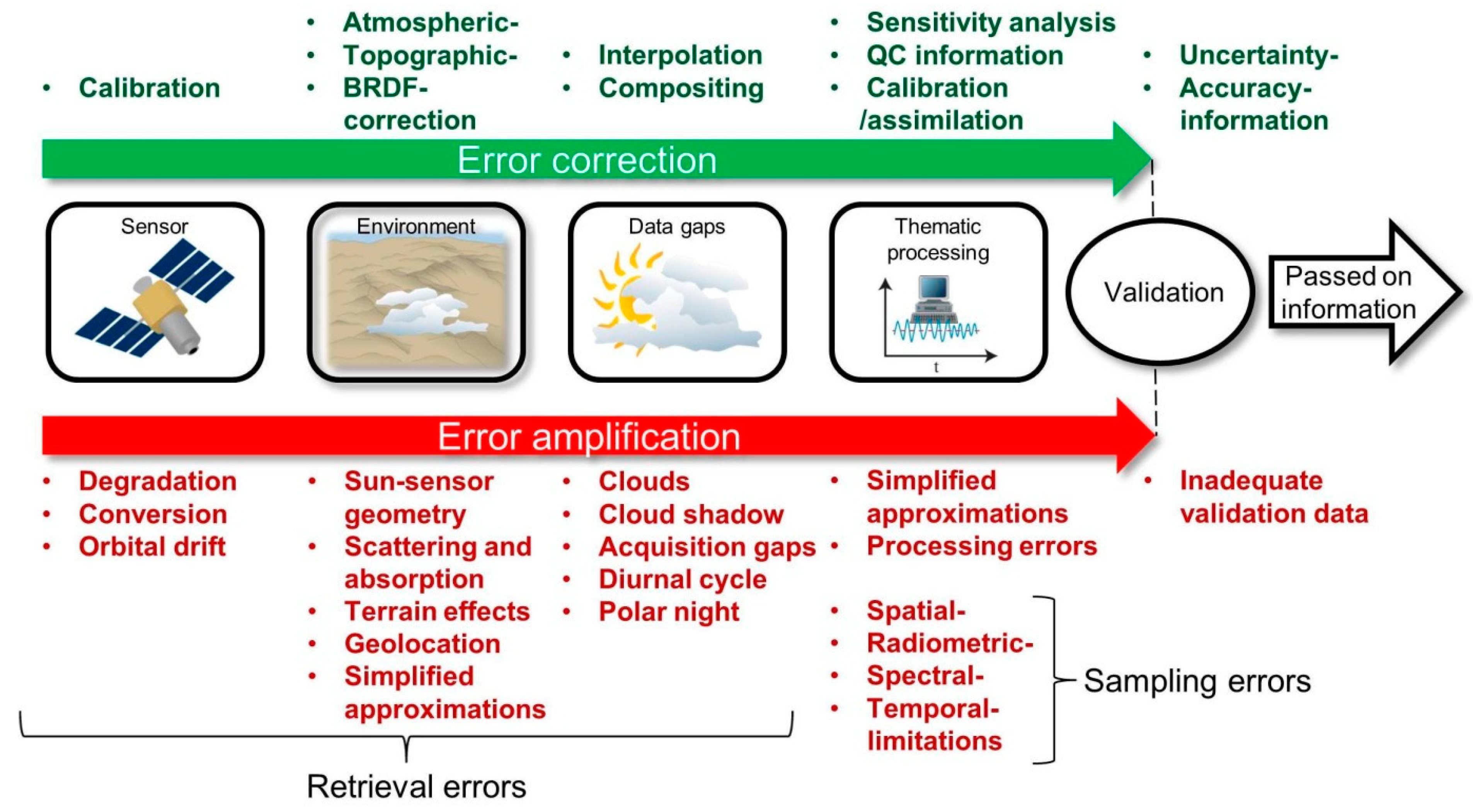
2.1. Main Error Sources of Remote Sensing Time-Series Products

Measurements of physical quantities are subject to uncertainty. Factors that affect measurements in the field of remote sensing cannot be held constant, resulting in variability of the repeated measurements. Contributions to uncertainty in satellite estimations can be based on manifold factors (e.g., retrieval errors, sampling errors, and inadequate calibration/validation data [51], Figure 4).

Satellite sensors need to convert the electromagnetic signal from earth in voltage and digital numbers in order to obtain reflectance or radiance values. For a reliable conversion, the constant calibration of sensors is essential [29,52] to counteract sensor-prone error sources (e.g., sensor degradation, different sensor sensitivity for specific bandwidths). For this purpose, modern instruments, such as MODIS, employ onboard calibration systems. Furthermore, deviations due to variable sun–sensor geometry and geolocation errors have to be attended to. Geolocation uncertainties can be an issue due to varying projection systems, target shift, or different point spread functions [53]. Additionally, orbital drift has to be taken into account, as, for example, the orbital drift of each National Oceanic and Atmospheric Administration (NOAA) satellite during their lifetime evokes a cooling effect in advanced very high resolution radiometer (AVHRR) LST products [54]. The next step is the correction of signal alternations induced on the path from the target to the sensor. Outgoing radiance consists of components affected by environmental influences and atmospheric absorption and scattering effects. To obtain surface reflectance information, atmospheric correction is commonly applied, along with topographic correction and bidirectional reflectance distribution functions (BRDFs). For passive microwave observations, man-made radio frequency interference is also able to contaminate signals [55]. Once the corrected data is accessible, successive error sources are introduced in the subsequent processing. Model uncertainties mainly relate to simplified approximations of natural variability [56] and data gap handling. Main causes for temporal inconsistency in optical remote sensing data are data gaps due to cloud cover. Data quality suffers under cloud and cloud shadow contamination by amplified variance and abnormal error distribution in the data [57]. Depending on the object of investigation, snow cover and coarse temporal resolution can also cause data inconsistency. To interpolate data gaps, several reconstruction models (e.g., harmonic analysis, double logistic, asymmetric Gaussian or Whittaker smoother, Savitzky–Golay filter) have been established [58]. Gap-corrected data, however, have the potential for implications in downstream applications, as incorporated uncertainty is carried further to subsequent models [28]. A different approach to gain consistent time-series presents value compositing (e.g., maximum value), where multiple images are processed for a preset period of time to create representative, cloud-free datasets with the least atmospheric attenuation and viewing geometry effects [59]. This can reduce the impact of missing data and unexpected day-to-day variations. However, the application of filters and compositing comes with the disadvantage of information loss and lower temporal consistency [48,55]. For regions with a high frequency of gaps (e.g., tropical areas), even composite products often contain extensive gaps, which has become increasingly problematic in areas where no alternative source of geospatial datasets is available [28]. To oppose ambiguous observations, quality control (QC) is used to provide information on the retrieval quality by flagging data acquisitions. This procedure adds quality indicators to the original observation without modifying or removing it [60]. As a result, the anticipation of systematic errors related to the shortcoming of retrieval algorithms and inaccurate prior knowledge [57] can be improved. Further accuracy-limiting factors are of a technological nature, concerning the sensor’s spatial (geometric), radiometric, spectral, and temporal resolution [61], which can be summarized as sampling errors. These errors become effective if information is assessed at a level of detail that cannot be properly sustained by the capabilities of the data acquisition mechanism.

Although an emphasis lies on the correction of known errors sources, complete compensation cannot be achieved. Myneni et al. [62] have shown, for instance, in LAI modeling, that even properly calibrated surface reflectance information obtained under clear sky conditions is still subject to independent variations due to measurement geometry, surface characteristics (e.g., snow, soil characteristics), and canopy cover. Eventually, results have to be accompanied by validation information to ensure proper interpretation. Furthermore, time-series need to show temporal stability in their accuracy, since changing data quality over time would justifiably concern users that temporal trends observed in the data are ambiguous [63].

2.2. General Considerations in Time-Series Validation

Validation presents means to assess implied uncertainties by analytical comparison to reference data. Uncertainty can be differentiated in physical and theoretical uncertainties [64]. Physical uncertainties represent the actual departure of product values from reference values, which are obtained through independent validation studies [32,65]. Theoretical uncertainties emerge from the inverse procedure as they relate mainly to uncertainties in the input data along with model simplifications and are usually estimated by individual product science teams to accompany the product with quality information (e.g., QC information) [21].

Primarily methods can be categorized into direct and indirect validation. Direct validation is based on the comparison with independent data sources, which are representative of the target or true value, enabling the absolute quantification of uncertainties (physical uncertainties). For geospatial data, direct validation is commonly accomplished at the pixel scale through the comparison of a product with independently acquired data, observing the same ground parameter coherent in time and location [66]. The required truthfulness of reference data, however, is not always met for the validation of geophysical measurement systems, as the data considered often include inherent measurement errors, biasing calibration and validation information [67]. Next to the quality of reference data, the amount of obtainable reference data is mainly a limiting factor for extensive spatial coverage of validation efforts [68]. Raw in situ data is typically available as point measurements, leading to biased assessments when compared to raster data [69]. As a consequence of the larger spatial resolution of satellite sensors, representative areas of ground observations have to be upscaled to approximate the target cell size. This principle is frequently applied to higher resolution satellite images to represent an estimation of the in situ state on a spatial grid and as an intermediate step for comparisons to data that has an even coarser resolution [65,70,71]. This two-stage process is subject to uncertainty itself, as the accuracy of ground-based reference maps depends on errors in field measurements but also on uncertainties of fine resolution satellite data, and sampling and spatial scaling errors [72]. On the other hand, for small-scale investigations based on higher resolution data, a direct comparison to interpolated in situ data time-series can be more viable [73]. Indirect validation is less affected by these constraints, using data with similar characteristics for an intercomparison of products. This procedure allows the evaluation of gross differences and possible insights into the reasons for variations [8] by considering the consistency of a given product relative to related data at a comparable spatial scale. The ease of application promotes indirect validation in the field of remote sensing, especially with regard to the temporal aspect of time-series, although absolute uncertainty is not achievable. As a major issue, temporal stability of validation outcomes is one aspect required by the Committee on Earth Observation Satellites’ Land Product Validation Subgroup [32]. To provide spatially and temporally consistent reference data, a vast network of calibration and validation sites has been established. Through the provision of independent measurements of relatable values over time, requirements for long-term direct validation can be met [74].

3. Characterization and Categorization of Reviewed Studies

Earth observation remote sensing time-series are based on spaceborne satellites with a corresponding sensor payload. A range of sensors were utilized in the reviewed studies (Appendix A of

Table A1. Abbreviations of sensors and journals.

Abbreviation	Full Description
AATSR	Advanced Along Track Scanning Radiometer
AMSR2	Advanced Microwave Scanning Radiometer 2
AMSR-E	Advanced Microwave Scanning Radiometer-Earth Observing System
ASCAT	Advanced SCATterometer
ATSR IRR	Along Track Scanning Radiometers Infra-Red Radiometer
AVHRR	Advanced Very High Resolution Radiometer
CERES	Clouds and the Earth’s Radiant Energy System
ERS Scatterometer	European Remote Sensing Satellite
GOES Imager	Geostationary Operational Environmental Satellite
MERIS	MEdium Resolution Imaging Spectrometer
MODIS	Moderate-resolution Imaging Spectroradiometer
MTSAT Imager	Multifunctional Transport Satellites
MVIRI	Meteosat Visible and Infrared Imager
PROBA-V	Project for On-Board Autonomy Vegetation
SeaWiFS	Sea-viewing Wide Field-of-view Sensor
SEVIRI	Spinning Enhanced Visible and InfraRed Imager
SMAP	Soil Moisture Active Passive
SMMR	Scanning Multichannel Microwave Radiometer
SMOS MIRAS	Soil Moisture and Ocean Salinity Microwave Imaging Radiometer with Aperture Synthesis
SPOTVGT	Satellite Pour l’Observation de la Terre Vegetation
SSM/I	Special Sensor Microwave/Imager
TANSO	Thermal and Near infrared Sensor for Carbon Observation
TM/ETM	Thematic Mapper/Enhanced Thematic Mapper
TMI	Tropical Rainfall Measuring Mission (TRMM) Microwave Imager
ADV SPACE RES	Advances in Space Research
AGR FOREST METEOROL	Agricultural and Forest Meteorology
BIOGEOSCIENCES	Biogeosciences
EARTH INTERACT	Earth Interactions
EARTH SYST SCI DATA	Earth System Science Data
ECOL APPL	Ecological Applications
GEOSCI MODEL DEV	Geoscientific Model Development
GLOB CHANGE BIOL	Global Change Biology
HYDROL PROCESS	Hydrological Processes
IEEE GEOSCI REMOTE S	IEEE Geoscience and Remote Sensing Letters
IEEE J SEL TOP APPL	IEEE Journal of Selected Topics in Applied Earth Observations and Remote Sensing
IEEE T GEOSCI REMOTE	IEEE Transactions on Geoscience and Remote Sensing
INT J APPL EARTH OBS	International Journal of Applied Earth Observation and Geoinformation
INT J DIGIT EARTH	International Journal of Digital Earth
INT J REMOTE SENS	International Journal of Remote Sensing
ISPRS J PHOTOGRAMM	ISPRS Journal of Photogrammetry and Remote Sensing
J APPL REMOTE SENS	Journal of Applied Remote Sensing
J GEOPHYS RES-ATMOS	Journal of Geophysical Research: Atmospheres
J GEOPHYS RES-BIOGEO	Journal of Geophysical Research: Biogeosciences
J HYDROMETEOROL	Journal of Hydrometeorology
REMOTE SENS	Remote Sensing
REMOTE SENS ENVIRON	Remote Sensing of Environment
REMOTE SENS LETT	Remote Sensing Letters
SOL ENERGY	Solar Energy

), showing various application domains determined by their technical characteristics (e.g., wavelength spectrum, revisit time, resolution, operational period). To outline the larger picture of scientific applications of temporally dense, large-area time-series products, quantitative information regarding the composition (sensors, variables) and research area is illustrated in the following subsections. The topic of validation in the scope of this review furthermore requires a generalization of complex validation strategies to enable a synthesized categorical overview of validation methods. Respective classification guidelines are explained in Section 3.3.

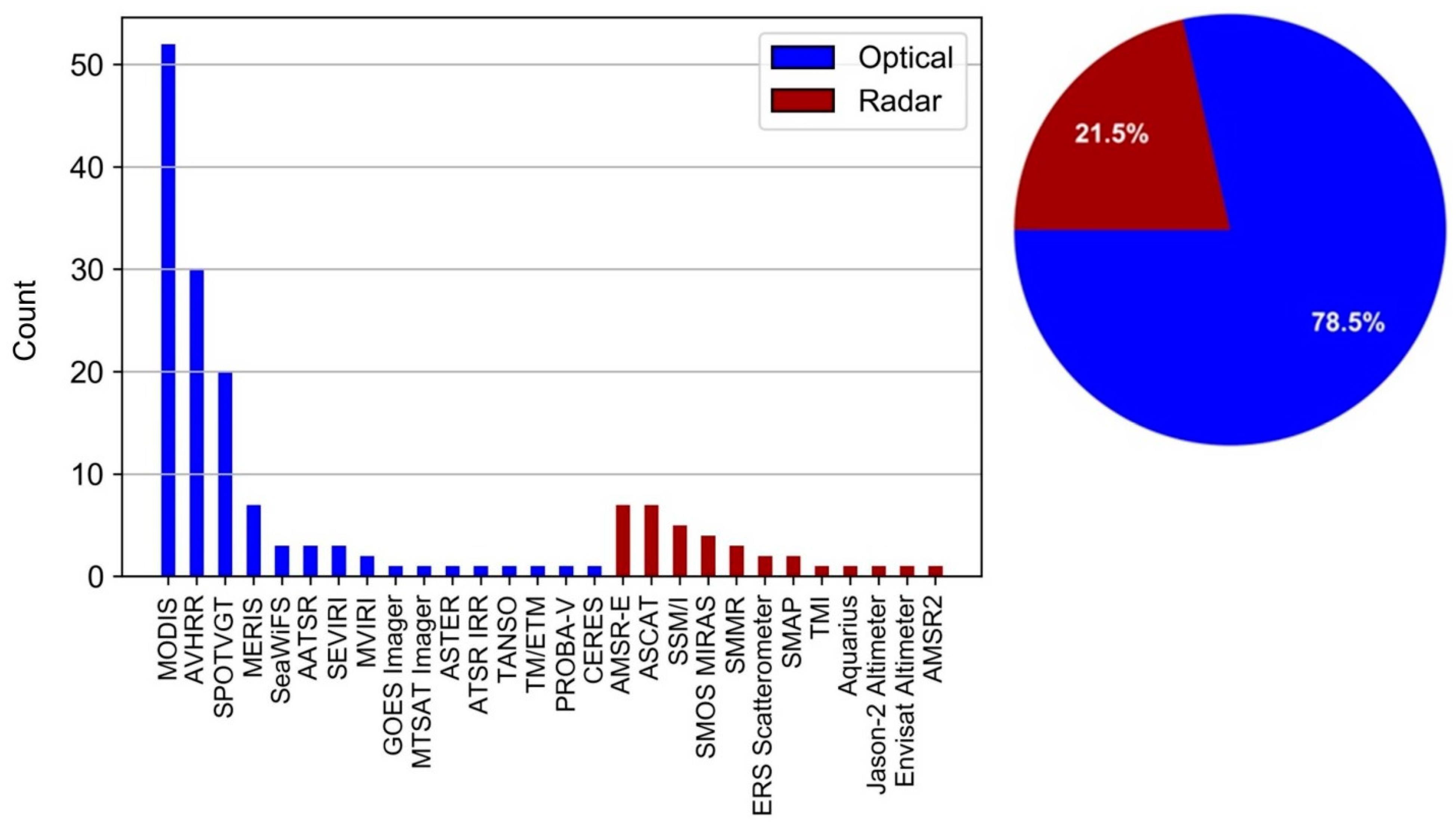
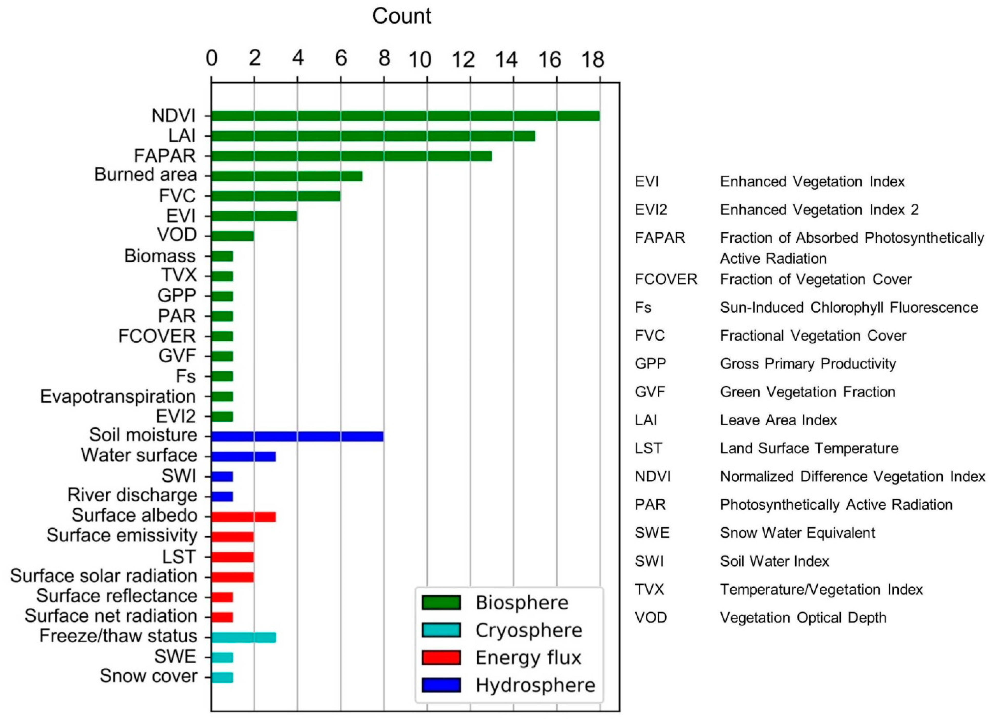
3.1. Preferred Sensors and Time-Series Variables

According to the operational frequency (or wavelength) bandwidth, sensors are principally distinguished in optical and radar domains. Operating in different frequency ranges offers various advantages for the investigation of certain variables [75]. Concerning the application of remote sensing platforms, the covered extent in combination with revisit times is also decisive. In the optical/multispectral sector, prominent examples within the reviewed studies are the AVHRR, MODIS, SPOTVGT, and Medium Resolution Imaging Spectrometer (MERIS). Sensors of the Landsat Data Continuity Mission (Multispectral Scanner MSS, Thematic Mapper TM, Enhanced Thematic Mapper Plus ETM+, Operational Land Imager OLI) were mainly used as higher resolution reference data, as was to a lesser extent Sentinel 2 data [76].

In this review, medium resolution optical sensors specially show high employment. MODIS data is most frequently used (52 studies). For the pre-MODIS era, AVHRR was the prevalent sensor for extensive global change studies because its visible red and near infrared channels enabled the estimation of NDVI from 1981 onwards [59]. Due to the utilization of MODIS, AVHRR, and SPOTVGT (Figure 5), the optical domain is generally represented to a much higher degree (78.5%) compared to radar-orientated research (21.5%). As the main focus of studies lies on vegetation, a large part of the investigations in the scope of this review are facilitated by the features of optical sensors. This is also reflected by the most frequently utilized variables (Figure 6). A relatively small fraction of the optical domain is furthermore constituted by the thermal sector, which is represented by AVHRR [77], MODIS [3,28,54], and AATSR [54] thermal infrared sensors.

In the radar domain, one of the primary sensors is the Advanced Microwave Scanning Radiometer-Earth Observing System (AMSR-E), although its data availability ceased in 2011. The same degree of utilization is seen for the Meteorological Operational Satellites (MetOp) Advanced Scatterometer (ASCAT), followed by the Special Sensor Microwave/Imager (SSM/I).

A variety of time-series-derived multitemporal variables have been employed in the studies (Figure 6). Mainly geophysical variables (defined by physical units) and index variables (dimensionless) were utilized. Thematic variables, which typically feature a larger amount of analyst bias [12], are found in burned area, water surface, and freeze/thaw status investigations. Overall, the majority of studies facilitated the analysis of vegetation-associated variables (71.8%). To access specific variables or implement validation with regards to other factors, additional datasets are required [21,78,79]. This led to a frequent application of auxiliary data (e.g., surface temperature, land cover, precipitation, or digital elevation models) along with primary time-series.

Investigation periods are dependent on continuous data products, which rely on the operational life of sensors or the successful transition to other data sources (e.g., Global LAnd Surface Satellite (GLASS) datasets for surface emissivity and albedo [6]). Concurrent (e.g., data fusion [48]) or successive use of data sources from several satellite systems has been shown in 42 studies, as the full exploitation of current EO missions proves beneficial to the fulfillment of user requirements in terms of spatiotemporal continuity, consistency, and quality. On the other hand, data inconsistency between multiple sources and/or sensors needs to be handled accordingly. A common approach to overcome this issue is the use of learning algorithms [34,48]. Also, the transmission to newer sensors has an effect on continuity (as seen by AVHRR platforms), giving an advantage to uninterrupted lifetime sensors, like MODIS, whose products are therefore considered superior to other long-term datasets (e.g., NDVI [22,80]). Especially, the intercomparison of several products for validation [21,26,81,82,83] relies on the use of multiple data sources.

The review of investigation periods has shown time spans from single years to several decades (Figure 7). The longest study period (34 years) is based on a combination of the primarily used sensors AVHRR and MODIS [84].

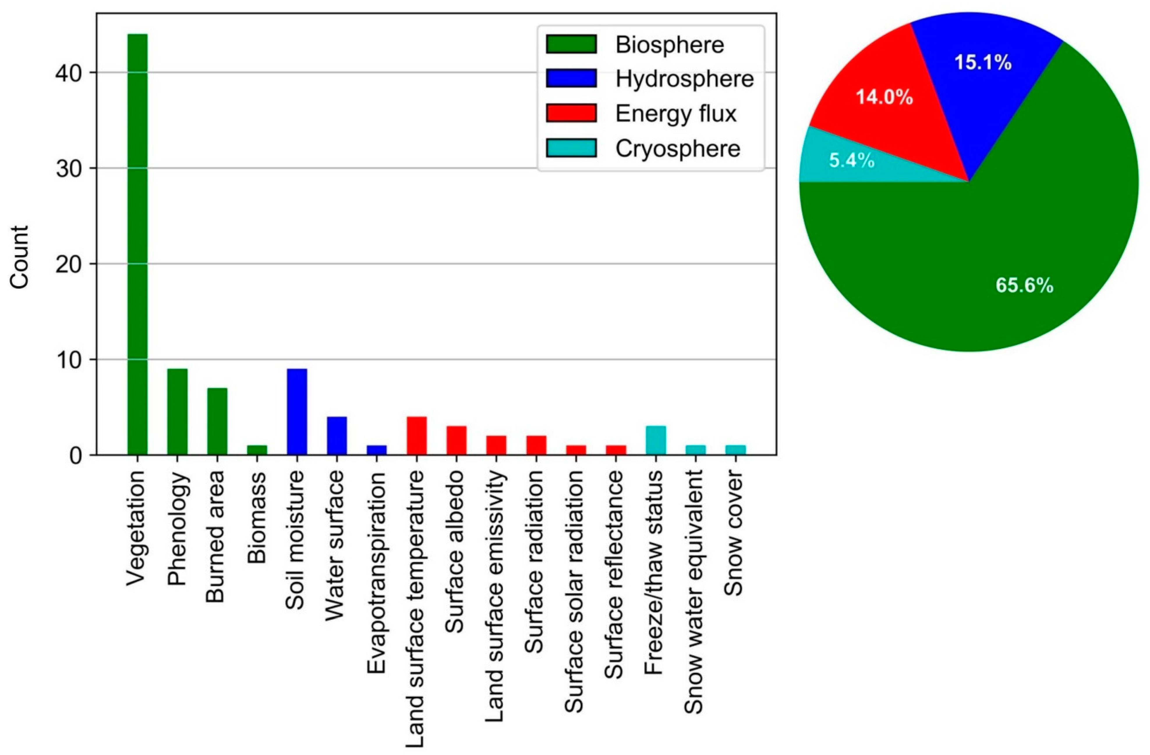
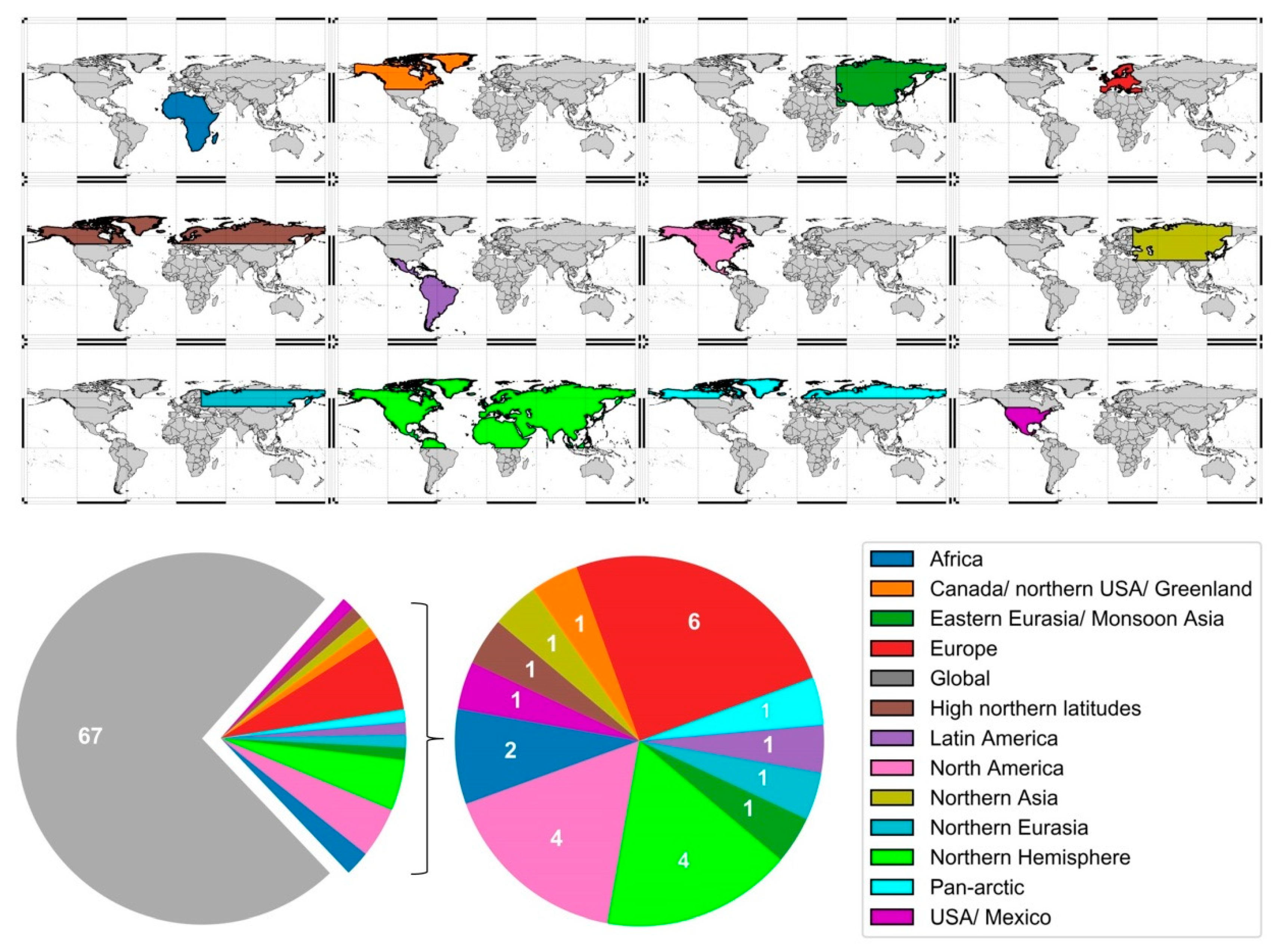
3.2. Thematic Foci and Spatial Distribution of Studies

Remote sensing time-series allow for the quantification of environmental variables and for the characterization of their temporal behavior on a global scale. Focus points of scientific research in this area were revealed by a categorization of studies according to research objects and affiliation to superordinate domains biosphere, cryosphere, hydrosphere, and energy fluxes (Figure 6, Figure 8). The results show a concentration on earth’s biosphere (65.6%) due to the frequent utilization of vegetation-related metrics, such as the NDVI, LAI, and FAPAR. The remaining categories constitute 34.4%, with soil moisture as the most frequently investigated topic outside the biosphere domain.

The spatial focus of studies is directed towards the global extent (73.6%, Figure 9). Valid coverage can be achieved by either explicit incorporation of the entire region of interest or by representation of well-distributed study sites [63,85]. Operating at a global scale comes with the advantage of enabling investigations of questions that are relevant to the global society by assessing global dynamics and relationships. As most studies operate on data sources that are generally available globally, the relatively small number of non-global investigations can be partly explained by the limited additional effort in expanding to the global extent. Pekel et al. [86], for instance, deliberately stated that their continental-scale implementation only represents the first step towards a global approach. In addition to a continental/global region of interest, a focus on local investigations, typically for locations of the available validation sites, can also be observed in the studies [39,87]. This enables product evaluations in higher detail, but the results are difficult to extrapolate to a larger extent, which is where validation data that better represent global characteristics become relevant [71].

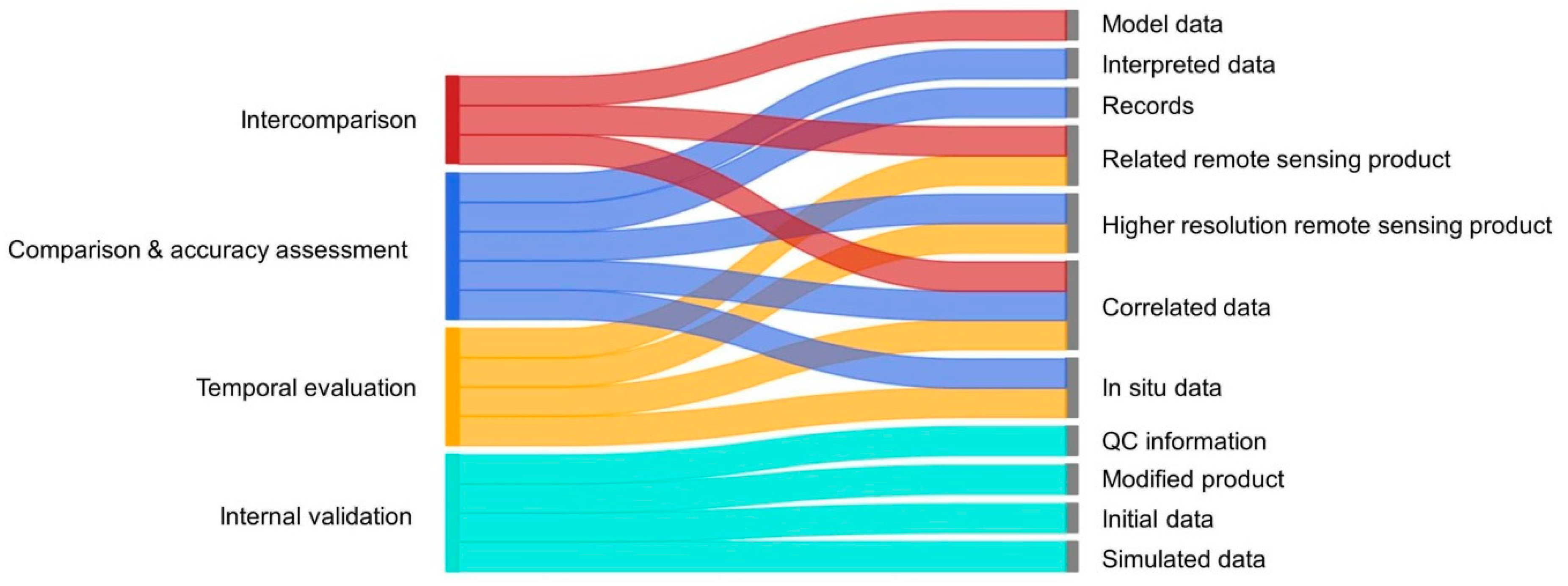
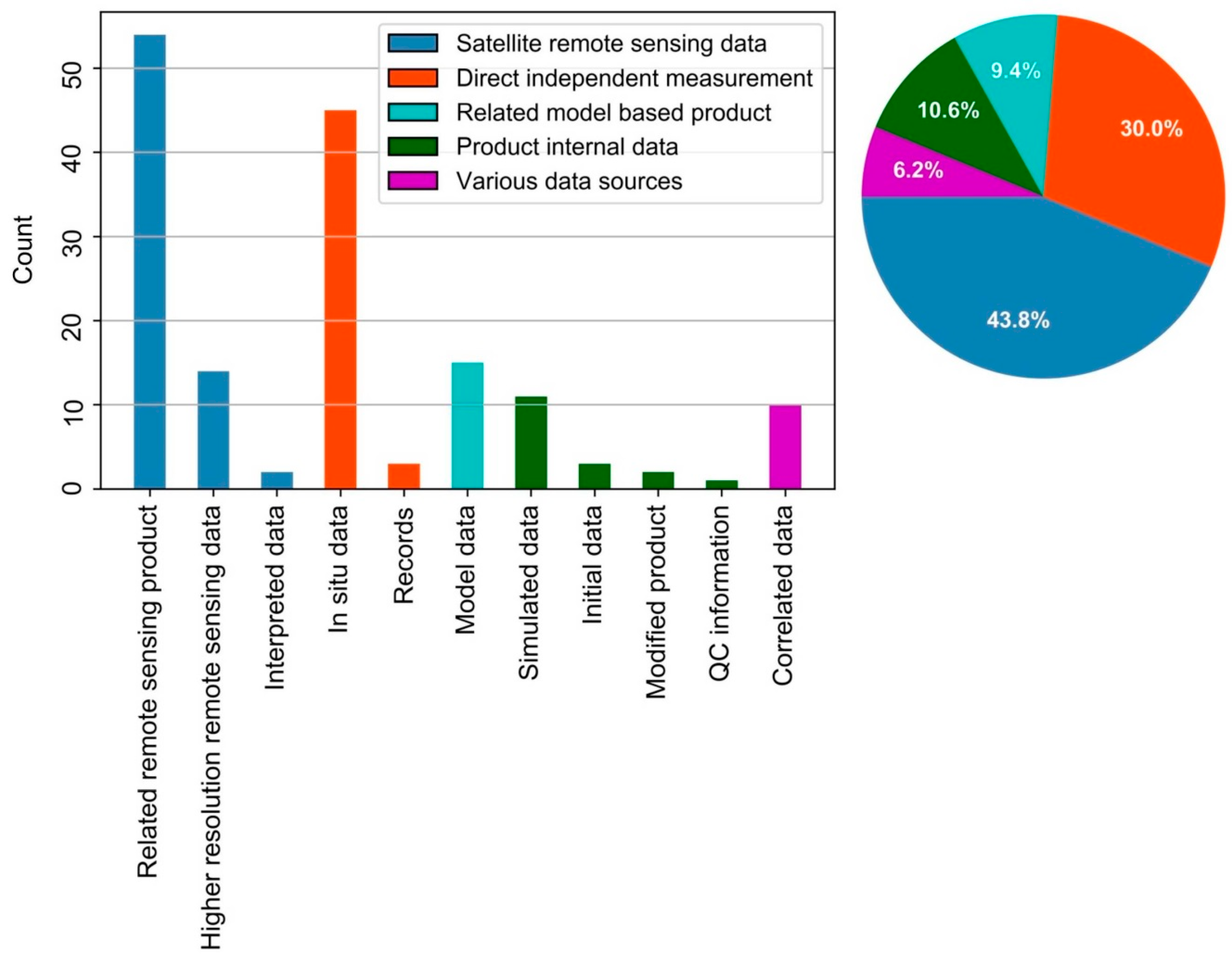
3.3. Categorization of Validation Approaches and Validation Data

The choice of validation method should be guided by the application of a product, since the purpose of a validation method is to quantitatively assess the performance of a dataset providing essential information to the user community [88]. The final determining factor, however, is the availability of validation data. The data situation (e.g., reliability, comparability, spatiotemporal coverage) also strongly influences the quality of validation results. The central criterion for the categorization of validation methods in this review is therefore the use of specific validation data (Figure 10).

To commence validation according to acknowledged standards [46], direct independent measurements are necessary. In this review, this type of validation is addressed as a comparison. This validation category includes methods that utilize reference data that feature significantly higher reliability regarding the true state of a measured variable. According to Congalton and Green [45], reference data has to be at least one level more accurate than the remotely sensed data and corresponding methods for product generation. Consequently, this excludes the use of similar data products in this regard. A comparison is typically accomplished by the use of in situ data, which represents the second most used data source for validation in the reviewed literature (Figure 11). In rare cases [89,90,91], historical or statistical records were also used as independent measurements for validation. A major disadvantage of ground-based observations is the limited spatial dimension. The evaluation of soil moisture by Chen et al. [92] has, for instance, shown that correlation coefficient metrics obtained from a comparison with point-scale ground observations underestimate the correlation between retrievals and true soil moisture values. For a reasonable comparison of raster data, point in situ data needs to be extrapolated to the satellite footprint or product grid scale. Further problems emerge in the requirement of independent ground measurements for a broad range of conditions (e.g., seasonal period of vegetation or atmospheric conditions [48]). This can limit validation opportunities to confined locations and/or discrete time periods [93].

A particular type of data used for validation is higher resolution remote sensing data. This kind of data can be utilized either to extrapolate in situ data on a spatial grid [94,95,96,97], downscale coarser data [95], or represent more accurate information regarding target values to gain adequate validation data [98,99]. In some cases, higher resolution remote sensing data is used in combination with only small-scale test sites [59], where pre-knowledge of land surface properties is available (e.g., homogeneity [100]). A further representation of reference data is manually interpreted data (e.g., photo-interpreted pixels [86]). This type of validation data is typically derived with the help of more detailed sources and can be assumed as the true state, if the manual identification of the regarding variable is reliable.

An established application for spatial data in terms of map accuracy is the implementation of an accuracy assessment. Since the application of this method only occurred by the use of reference data to execute cross tabulation, it can be allocated to the comparison category in this review. Because of the common application and relevance in remote sensing, accuracy assessments are listed here as a separate category. Based on this approach, several validation measures are obtained (e.g., commission error, omission error, overall accuracy, dice coefficient, Kappa), which consequently offer a deeper insight into the type of classification accuracy/error [44,45].

Apart from comparing the quantities of target values, it is furthermore possible to establish temporal relations between validation data and remote sensing time-series in temporal evaluations (e.g., transition date comparison [85]). Here, temporal evaluations have to be distinguished from the evaluation of the temporal stability of time-series, which can be assessed by various validation methods (e.g., intercomparison [82], generation of artificial data for assessment [101], change of accuracy through time [63]). Temporal benchmarks for temporal evaluations can be derived from various time-series data sources by applying further analysis and processing. In the case of in situ-based temporal information, temporal evaluations face similar issues to conventional comparisons, as additional uncertainties emerge from equating satellite acquisitions to in situ measurements (e.g., phenological dates [102,103]). A more straightforward approach for temporal evaluations is realized by the use of related time-series products [104,105].

Related datasets with similar spatiotemporal characteristics represent relatively uncomplex implementations for validation on continental to global scales due to the ease of matching coherent data points for validation. Quantitative product-to-product validation approaches are referred to as intercomparison in this review. In general, product intercomparisons are unable to deliver direct validation metrics relative to the ground truth but can provide metrics that indicate relationships to a chosen reference product with intrinsic uncertainties. Similar products are characteristically derived from external data sources. Here, this concluded in the sources of related remote sensing products, model data, and correlated data. A special form of intercomparison is triple collocation (TC). The administration of TC enables the estimation of error variances of a geophysical measurement system; however, it only provides relative error metrics [93]. For implementation, a reference dataset has to be chosen from three collocated data products with assumptions of linearity, signal and error stationarity, error orthogonality, and independence of errors in the constituent datasets [106]. The resulting error variances are consequently subject to the multiplicative and additive biases of the reference dataset [92].

Validation has also been accomplished by the use of datasets containing variables correlated to the primary time-series (correlated data). The use of correlated data has been seen for all methods facilitating external data sources. Accordingly, this data originates from in situ measurements [54,78,107,108,109,110] or has its source in external models or databases [78,110].

Internal methods are represented in this paper as techniques for validation without the support of additional external validation data [63,101,111]. Internal validation data is available either from the product generation process (initial data, QC information) or derivation from input/output data (simulated data, modified product). Information gained by this approach is based on the intrinsic validity of the product and has been applied in this review within four validation methods (Figure 12). The use of artificially produced validation data refers mainly to synthetic assessments but can also be applied in sensitivity analysis. QC information provides the basis for quality assessments while specific uncertainty/error estimation features unique validation approaches on an internal data basis. As this approach is independent of external data for validation, internal validation stands apart from previously presented validation methods.

4. Review of Validation Methods

Validation methods can represent complex procedures for the assessment of time-series products. A generalized overview of validation approaches realized in 89 reviewed studies is given in the following subsections. Particular examples are emphasized over standard implementations in order to outline the application spectrum of a category. Since various studies accommodated more than one validation technique, multiple category designations according to context can occur.

4.1. Validation by Intercomparison of Related Products

Intercomparisons of related data products are shown in a variety of studies in this review [23,24,25,26,76,87,90,96,112,113,114,115,116,117,118,119].

Along with similar remote sensing products for this type of validation, products in the form of model outcomes featuring the same target variable are also considered [120,121,122]. For instance, Albergel et al. [123] intercompared a fused radar soil moisture product with two reanalysis datasets. In addition to the intercomparison of AVHRR and MODIS NDVI time-series, Fensholt and Proud [22] also intercompared both MODIS sensors on Aqua and Terra satellites for an enhanced view on the validation results, showing the possibility of intercomparison from a sensor-internal aspect. Zhang et al. [29] also intercompared different versions of MODIS NDVI and enhanced vegetation index (EVI) datasets (Collection 5 and 6).

Furthermore, intercomparisons can be achieved by the use of correlated data. For example, Jones et al. [78] intercompared a vegetation optical depth (VOD) time-series with LAI, NDVI, and EVI data products. Zhang et al. [29] investigated the correlations of a global EVI dataset to three modeled key climate factors (radiation, air temperature, and precipitation) by conducting partial and multiple correlation analyses. A special case of intercomparison is presented by Tarnavsky et al. [100], who facilitated semi-variogram modeling to investigate the spatial variability of multiscale NDVI products for specific validation sites. By semi-variogram modeling, an assessment of the internal spatial variability of a spatial dataset by determination of characteristic properties, like the sill and the mean length scale metric, is enabled.

A special realization of product intercomparison is TC. In remote sensing, TC has been applied, in particular, for soil moisture products [64,112,114] but is also used for other subjects. D’Odorico et al. [21] obtained RMSE estimates from TC for their FAPAR product, using three spatially and temporally collocated datasets, assuming that they represent the same physical quantity and contain uncorrelated errors. Gruber et al. [124] used TC to merge active and passive radar soil moisture retrievals under consideration of the error characteristics of the individual data. Chen et al. [93] utilized TC to initially intercompare three radar soil moisture products to further extend this method to a quadruple collocation, in order to estimate error cross-correlations, facilitated by in situ site observations as a fourth soil moisture dataset.

More uncommon correlated data sources for intercomparison have been implemented by Rodell et al. [79], who conferred biomass changes to gravimetric remote sensing data from the Gravity Recovery And Climate Experiment (GRACE), or Suzuki et al. [125], who used modeled evapotranspiration data for the validation of NDVI time-series.

4.2. Validation by Comparison to Reference Data

Comparisons to reference data were mainly based on the comparative use of in situ data representing the same target variable. In this review, various examples outline this kind of validation approach [6,18,81,126,127,128].

Others utilized correlated in situ data for comparisons. Examples are found by the use of air temperature for the validation of freeze/thaw cycles [108,110] or LST [54], as well as datasets correlated to the water surface extent (in situ river discharges, water level heights, and precipitation estimates [109]).

Furthermore, higher resolution remote sensing data is eligible for comparisons. Considering the validation of a burned area product, Chuvieco et al. [98] visually analyzed higher resolution remote sensing data to gain interpreted data for comparison. Site-specific higher resolution data has been utilized to compare vegetation indices (fractional vegetation cover (FVC) [129], NDVI [59], LAI [94]), offering the advantage of more homogenous reference sites. Also, a combination of higher resolution data and in situ data is used, inter alia for converting in situ information to the spatial grid of higher resolution data [94,95,96,97]. Moreover, Wang and Liang [57] calibrated higher resolution data with the help of in situ information to produce more accurate grid data.

Records from statistical databases or historical events are another form of reference data that can be used for comparison. For example, records of crop yield per country were utilized by Zhang and Zhang [91] for a comparison with satellite-based estimates. Although not implemented as a validation strategy, Chuvieco et al. [76] compared their results with official fire statistics in addition to the intercomparison to other burned area products.

4.3. Accuracy Assessment

Accuracy assessments are grouped with comparisons by also utilizing reference data for validation (Figure 10) but are addressed separately in this review due to the relevance of this approach in the field of remote sensing. Several studies implemented accuracy assessments by means of cross tabulation between product and reference maps, allowing the generation of error or confusion matrices [98]. Some studies utilized learning algorithms as a central element of their product generation [34,39,48], although only Ramo et al. [90] employed a fraction of the training dataset ground truth in their accuracy assessment, which is based on higher resolution remote sensing data. In the case of burned area products [63,76,88,130], higher resolution remote sensing data (multi-temporal image-pairs) can satisfy the need for ground truth information. For water surfaces, Pekel et al. [86] used photo-interpreted samples of the input dataset as reference data for the computation of a comparison matrix. Klein et al. [131] furthermore considered a division of reference data (Landsat 8 higher resolution data) for their accuracy assessment of water surfaces according to the water sub-pixel content of the input image, thereby allowing more profound insight regarding the classification capabilities of their approach. Dietz et al. [132] used several accuracy assessments to reveal the different performances of particular steps in their cloud interpolation strategy. Padilla et al. [63] further investigated the trend of outcomes of their accuracy assessments over time, targeting temporal stability.

4.4. Temporal Evaluation

The temporal evaluation of certain points in time-series has been performed on the basis of various data sources in the reviewed literature [24,99,101,133]. Utilized temporal events originate from ground observations [39,134], records [89], or other data products [104,107]. Also, specific temporal indices, such as the growing season index (GSI), were used [78]. Consequently, temporal evaluations can be based on the principle of comparisons, intercomparisons, or both methods, given the provision of concurrent validation data [83,85,105]. Sobrino and Julien [99] employed resampled higher resolution remote sensing data of selected ground control points to validate long-term NDVI time-series in a temporal fashion. A further time-related example is the use of a time-series product as extreme event indicators (drought indicator [87], wildfires [135]).

4.5. Internal Validation

For synthetic assessments, validation data can be generated by modifying the original input to compare, for example, filtering methods [94] or by inserting artificial values (e.g., gaps, noise) into known input time-series in order to assess the capabilities of a model/algorithm [3,28,58,63,101,132,136,137]. Such methods were typically implemented if the study focused on improving distorted [111] or discontinuous time-series [94]. For instance, to examine the performance of their temporal stability analyses, Padilla et al. [63] created hypothetical burned area products.

For internal quality assessments, validation is accomplished by the use of quality information (QC information [21,108]), which is provided along with certain products (e.g., MODIS surface reflectance data) as ancillary data; however, this merely accesses theoretical uncertainties. For instance, Weiss et al. [9] assessed the continuity of a product as the fractions of valid and non-valid data as well as their distribution in space and time.

Some studies practice rather unique ways to quantify errors or uncertainties, which are designated as specific uncertainty/error estimation methods in this review. Typically, such estimations come with their own method and corresponding metrics (e.g., overall reconstruction error, fitting method-related error, gap-related error [58], predictive standard deviation [39]). For instance, Baret et al. [34] estimated the uncertainty based on confidence intervals applied to data points in the input training dataset. Weiss et al. [28] quantified uncertainty regarding fill distance errors related to gaps in the time-series. A similar principle was applied by Zhou et al. [137], who divided the overall reconstruction error into gap-related and fitting method-related error. In a later study, noise-related errors were also assessed [58]. Garcia-Haro et al. [39] estimated the predictive standard deviation, which quantifies the confidence on an associated estimate by penalizing outlier pixels. Particular cases of internal validation are the studies of Higuchi et al. [77] and Kumar et al. [138]. The first example used the AVHRR surface temperature and NDVI time-series to calculate temperature/vegetation regression slopes and the second presented an evaluation of soil moisture retrieval products using information theory-based metrics. These metrics rely on time-series analysis of soil moisture retrievals to estimate the measurement error, level of randomness (entropy), and regularity (complexity) of data.

Another applied internal method to provide information regarding the validity of results is sensitivity analysis. This method can provide estimates on the influence of parameters inherent to product generation. For this purpose, Keersmaecker et al. [111] used Monte Carlo simulations to execute a sensitivity experiment for simulated global NDVI time-series, in order to obtain accuracies as a function of the time-series characteristics and noise levels. The results could be applied to the original time-series and thus give a measure of reliability. Jones et al. [78] assessed the impact of algorithm assumptions on expected VOD retrieval accuracy based on error sensitivity analysis. For radar-based soil moisture estimation, Rodriguez-Fernandez et al. [139] investigated the sensitivity of their neural network to input specifications and soil temperature data to find the best input data configurations as well as the highest correlation to a reference product. For the estimation of river discharge, Sichangi et al. [140] also used, together with remote sensing altimetry data, information regarding river widths. Since the measurement error for the latter input is larger, a sensitivity analysis was conducted to improve the understanding of the validation results gained by comparison with in situ discharge. Garcia-Haro et al. [39] performed a sensitivity analysis to investigate uncertainty sources in retrievals by varying the cardinality of the training dataset, and in another experiment, assessed the uncertainties caused from different BRDF model parameters by the Monte Carlo method.

4.6. Combination of Methods

The majority of reviewed studies (61) facilitated more than one validation method. Hereby, a variety of studies showed, in particular, the combination of an intercomparison of products with a comparison to reference data [9,21,35,48,53,54,57,59,84,97,120,121,122,123,124,129,133,135,139,141,142,143,144,145]. This dual approach can provide an indication of general remote sensing performance for a particular research area or, on the other hand, illustrate improvements of novel methods in relation to existing products [35,71,136].

Several examples outline the successful combination of methods. For instance, Liu et al. [143] validated the GLASS albedo product by comparison with similar MODIS data as well as globally distributed ground measurements. To further improve validity, intercomparisons can also be spatially limited to the validation areas where in situ information is available [21,71]. The comprehensive accuracy assessment of global burned area estimations by Chuvieco et al. [76] was also subject to intercomparison, since the globally distributed ground truth information is furthermore suitable for the validation of other global products. A similar approach of intercomparing outcomes of standardized accuracy assessments was accomplished by Padilla et al. [88]. For the temporal evaluation of FAPAR time-series, Forkel et al. [104] conducted intercomparisons of products to gain deeper insights into temporal discrepancies. Another approach to conduct a spatiotemporal intercomparison is the use of three-dimensional voxel grids, defined both in space and in time, for validation [82]. Garcia-Haro et al. [39] combined a multitude of methods (sensitivity analysis, specific uncertainty/error estimation, intercomparison, comparison), as they initially included specific uncertainty estimates taking into account the uncertainty captured by the retrieval method and input error propagation and subsequently conducted an intercomparison with other satellite-derived products and comparison based on in situ measurements.

5. Summary of Validation Methods in the Reviewed Literature

The evaluation of the applied validation methods clearly showed two mainstream validation approaches for large-scale temporally dense earth observation time-series (Figure 12). These methods primarily relied on related remote sensing data for intercomparison and in situ measurements for comparison (Figure 11). The implementation of the remaining validation categories (temporal and internal) in the investigated studies constituted to 24.3% of the studies. Notably, the combination of several validation methods in single publications was prevalent. A typical implementation was the large-scale intercomparison of related products with a parallel focus on comparisons to measurements of specific validation sites.

Furthermore, the application frequency of methods according to research objects was analyzed, revealing the universal utilization of comparisons and intercomparisons along study subjects (Figure 13). As the primary field of application, vegetation-focused studies were mainly validated by these conventional methods but also became subject to internal procedures. Other distinct patterns are shown for thematic-related phenology studies, which typically incorporated temporal evaluations, while soil moisture studies showed an emphasis in the field of TC, and burned area results were mainly validated by accuracy assessments.

5.1. Expression of Validation Results

A variety of performance metrics are used for the validation of remotely sensed estimates of variables. Although metrics are often related, they come with advantages and disadvantages as no single metric or statistic can capture all the attributes of environmental variables [146]. Regularly used terms throughout the studies are well-established metrics, which can provide a measure of agreement between the product and reference. The most frequently used metric is the RMSE (Figure 14), which, in the case in which it is computed between ground measurements and product values, indicates the accuracy or total error. Following this are measures that originate, to a large part, in linear correlation as well as statistical hypothesis testing and other basic statistical terms. By the statement of correlation (e.g., coefficient of determination, R²), an indication of the spatial and/or temporal relation between products and reference is provided rather than an absolute expression of agreement. The standard deviation of the difference between product and reference data pairs can report on the precision of a product generation process. In the case of linear regression, the slope and offset deliver information on possible bias. The statistical significance of results is frequently provided along with the results, giving additional knowledge about the validity in terms of the probability that outcomes occur by chance. A subset of used terms is especially suited for assessing spatial data (i.e., pixel level, Figure 14) and are largely known for their application in accuracy assessments [130]. Furthermore, common graphical methods for the illustration of validation-related issues are frequently shown. Accordingly, plots of temporal profiles and map comparisons are often used to illustrate temporal and spatial differences of datasets. The choice of metric is, on the one hand, influenced by the nature of observations as well as characteristics of the science application and its sensitivity to the retrieved environmental variable [147] and, on the other hand, by the chosen validation method (e.g., metrics typically used for spatial data). For instance, when conducting an intercomparison of products, it seems more adequate to assess the correlation among products rather than the determination of absolute differences between datasets containing respective uncertainties.

5.2. General Trends

The number of studies that implement large-scale remote sensing time-series with associated validation has increased in the last two decades. This might be partly caused by the commission of the two MODIS satellites (Terra 1999, Aqua 2002). Concurrently, the diversity of validation methods has also increased (Figure 15). In the first 10 years of the 21st century, mainly comparisons, intercomparisons, and temporal evaluations were conducted. After that, internal validation methods were more frequently applied, along with the upcoming usage of TC and large-scale accuracy assessments. Yet, the majority of studies in the scope of this review still rely on conventional approaches. This might be facilitated by the increasing number of available products for intercomparisons. Also, comparison approaches benefit from the improved effort of the systematic provision of reference data by global validation networks. For the year 2019, only one recent study could be incorporated in this review [84], which features a combination of the mainstream validation methods. A general trend towards higher variability in the application of different categories of validation methods along with a rising number of suitable studies can mainly be observed after 2011, concerning primarily internal methods.

6. Discussion on the Challenges and Implications of Validation

In this review, studies were investigated that cover large-area and temporally dense remote sensing time-series that feature validation efforts for their outcomes. In terms of the applicability of validation approaches, the scope of this review represents challenging circumstances regarding the spatiotemporal availability of adequate validation data. The hereby favored validation approach is the intercomparison of products (indirect validation). A main strength of this procedure is the similar spatiotemporal extent that related remote sensing products usually share, making it comparatively easy to evaluate consistencies/differences coherently in space and time over large areas representative of various global conditions [35]. On the contrary, it lacks a link to quantitative reference data [68], implying the inability to investigate absolute errors with respect to the true state. The same principle is observed with TC. This procedure can be used as a complementary method to estimate theoretical uncertainties. Further challenges for the application of TC is the incorporation of different kinds of datasets (in situ measurements, satellite observations, and model fields) as they refer to different scales. By using satellite remote sensing triplets, the requirement of uncorrelated errors becomes problematic [21]. However, the inclusion of a fourth independent dataset can help meet this requirement [148]. Implementations as extended triple collocation [67] are able to yield the correlation coefficient of the measurement system with respect to the unknown truth, thus not requiring a reference dataset.

To address the requirements of global change communities (e.g., [2]), physical uncertainties obtained from direct validation are needed in order to obtain total uncertainty [21]. To conduct validation of remote sensing data according to recognized criteria [46], independent data (e.g., in situ data) are essential. Validation approaches that follow this guideline can be found in the comparison and accuracy assessment categories in this review. For the categorization of these validation methods, the main defining criterion is the use of reference data, which is expected to approximate the true state of a measured variable with considerably smaller uncertainty than the assessed product. The main data sources that meet this requirement are ground observations. Yet, in situ data contains measurement errors as well. In certain cases, uncertainties account for 10% to 30% (evapotranspiration estimates by eddy covariance flux towers [20]). However, they can be considered insignificant compared to those of most major remote sensing retrievals (e.g., soil moisture [138]). Furthermore, the implementation of confusion matrices in accuracy assessments is limited by the preciseness of the class definition [50].

Another common source for reference data is higher resolution remote sensing images, as this approach is recommended, for instance, by the CEOS CalVal protocol for burned area products [76,149]. Respective data are subject to established errors in the field of remote sensing as well. Nevertheless, by using adequate means for the derivation of reference information, it can represent independent, detailed, and accurate validation data [59].

Alternatively, networks of validation sites could cover the need for extensive reference datasets. Several studies refer to validation sites as the origin of their validation data, with common examples like BEnchmark Land Multisite ANalysis and Intercomparison of Products (BELMANIP), VAlidation of Land European Remote sensing Instruments (VALERI), and FLUXNET sites. Due to several well-distributed networks, it is already possible to match the spatiotemporal requirements to validate time-series of certain variables by the use of reference data (e.g., LAI, FAPAR [150,151]). However, the capabilities of major validation networks for covering the variety of geophysical variables are limited. This consequently constrains the investigation spectrum to products that target identical or explicitly correlated variables. The combined use of multiple networks in global studies (e.g., soil moisture [60]) is further complicated by a lack of standardization and protocolling. A major aspect regarding the usage of reference data is the spatial and/or temporal scale difference to time-series products, as it is challenging for field observations to be representative of coarse raster data cells (e.g., MODIS pixel [94]). Additionally, the location of coarse pixels and ground data may not match because of geo-location uncertainties [152]. Methods to overcome scaling issues have been shown by several studies, but eventually, sampling errors are not completely avoidable.

Other studies are focused on the temporal aspect of validation, shifting the emphasis from quantitative investigations to distinctive temporal behaviors of time-series. This approach is particularly vulnerable to continuity distortions (persistent cloud cover, high levels of atmospheric aerosols), weak seasonality of investigated variables, and insufficient temporal sampling of remote sensing sensors to capture rapid transitions (e.g., phenology studies [85,153]). This kind of assessment merely reveals validity in terms of timing, as no absolute uncertainty in the form of measured quantities is targeted. On the other hand, valuable information can be identified when validation using ground measurements fails to capture potential issues [121].

Although advances in the use of extensive calibration and validation networks for specific geophysical variables have been made, the central issue of validation remains in the acquisition of appropriate reference data. There is still a lack of ground measurements representative for sufficiently long time periods to fully utilize quantitative assessments [6,48]. Also, a need for more in situ measurements in specific regions makes the evaluation of products challenging (e.g., areas north of 60° [25]). Although more demanding in implementation, only direct validation by the use of reference data enables the assessment of physical uncertainties and it may be argued that only such methods can be seen as actual validation in the field of remote sensing. As part of this review, a variety of means to assess the validity of remote sensing time-series are considered as relevant methods.

An opportunity is given for internal validation methods, for which validation data is inherent to the product or might be generated by simulations based on available information. Simulations of time-series provide an additional approach, particularly for testing temporal analysis methods in a controlled environment [154]. As for intercomparison, internal methods are not able to provide a total measure of uncertainty but enable an internal estimation of model/algorithm performance. Nevertheless, a generic virtue of product internal validation data is the complete coverage of the product extent, both in space and time.

Apart from only using a single validation method, a strong inclination towards facilitating more than one approach is observed. By combining methods, an improved information content of the validation results is achievable. However, diverging outcomes have to be expected for the execution of a number of validation methods. This has been shown by D’Odorico et al. [21], as three diverse validation methods (comparison, intercomparison, internal validation) resulted in different validation outcomes. Additional discrepancies in validation results can be implied by means of different sampling strategies for reference data. Various studies placed an emphasis on the distribution of their validation efforts to distinct validation locations according to scale, land cover, biome type, or climatic setting in order to account for expected variability over the globe [54,57,101,115,116]. As pointed out by Cescatti et al. [81] in the case of the investigation of surface albedo, a weakness of in situ sites can be inhomogeneity. This further highlights possible discrepancies of validation outcomes according to applied approaches and demonstrates that, in practice, a validation approach might not produce the universally best results but should address product features relevant to the final product user [130]. An overview of general considerations regarding the validation method categories in this review is given in

Table 1. Advantages and disadvantages of validation method categories.

Validation Method	Advantages	Disadvantages
Comparison	Direct validation Physical uncertainties Assessment of quantitative errors	Need for independent acquisitions Complex spatiotemporal matching of validation data
Accuracy assessment	Adapted for spatial data Thematic map comparison with corresponding metrics Well established in remote sensing	Precise definition of classes necessary 1
Intercomparison	Simplified spatiotemporal approximation of other data products	Indirect validation Only relative error metrics
Internal validation	Spatiotemporal match of validation data Directly accessible validation data Synthetic assessments well suited for interpolation methods	Theoretical uncertainties Validation outcomes are dependent on product properties
Temporal evaluation	Straightforward comparison of extensive datasets	Vulnerability to continuity distortions, weak seasonality and insufficient temporal sampling Only validity in terms of timing

¹ Accuracy assessments share the same disadvantages as regular comparisons.

.

As validation is an essential component of any earth observation product, some studies still do not facilitate validation efforts. In the reviewing process of this paper, several publications failed to meet the requirement of a distinct expression of validation efforts and corresponding results. This brings attention to the controversial issue of the need for validation, especially for products that are generated by the use of already validated time-series, and error propagation is marginal due to the simple processing of input.

7. Conclusions and Outlook

This review presented an overview of the validation approaches of studies that utilize large-area, temporally dense earth observation time-series of land surface variables since the year 2000. Along with validation strategies, quantitative information on data basis, thematic foci, and spatial distribution were also investigated. Encountered validation methods were categorized according to the utilized type of validation data. The resulting classes incorporate a comparison to reference data, including accuracy assessments, the intercomparison of related data products, product internal validation, and temporal evaluation of time-series. The scope of this review led to the following key findings:

• The main data sources of studies are optical sensors (78.5%), with MODIS, AVHRR, and SPOTVGT as major contributors.
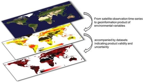
• The dominant thematic focus is on vegetation-orientated variables (71.8%), mainly represented by time-series of NDVI, LAI, and FAPAR.
• An emphasis on a global coverage of studies is prevalent (73.6%).
• The main sources of validation data are related remote sensing products (33.7%) and in situ data (28.1%).
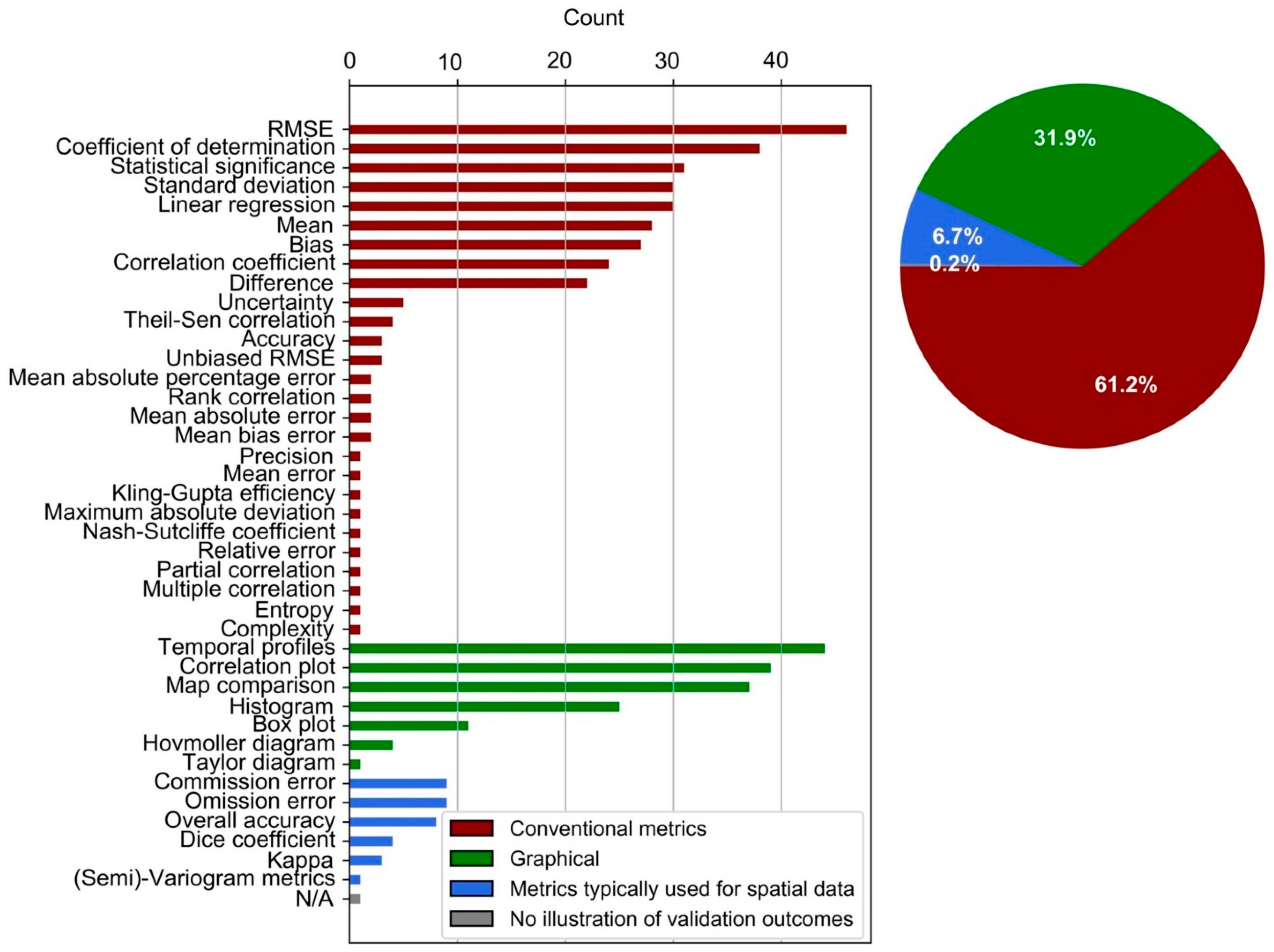
• For the expression of validation outcomes, conventional metrics or correlation-based metrics (RMSE, R²) are mostly calculated, along with a frequent presentation of graphical illustrations of temporal profiles, correlation plots, and map comparisons.
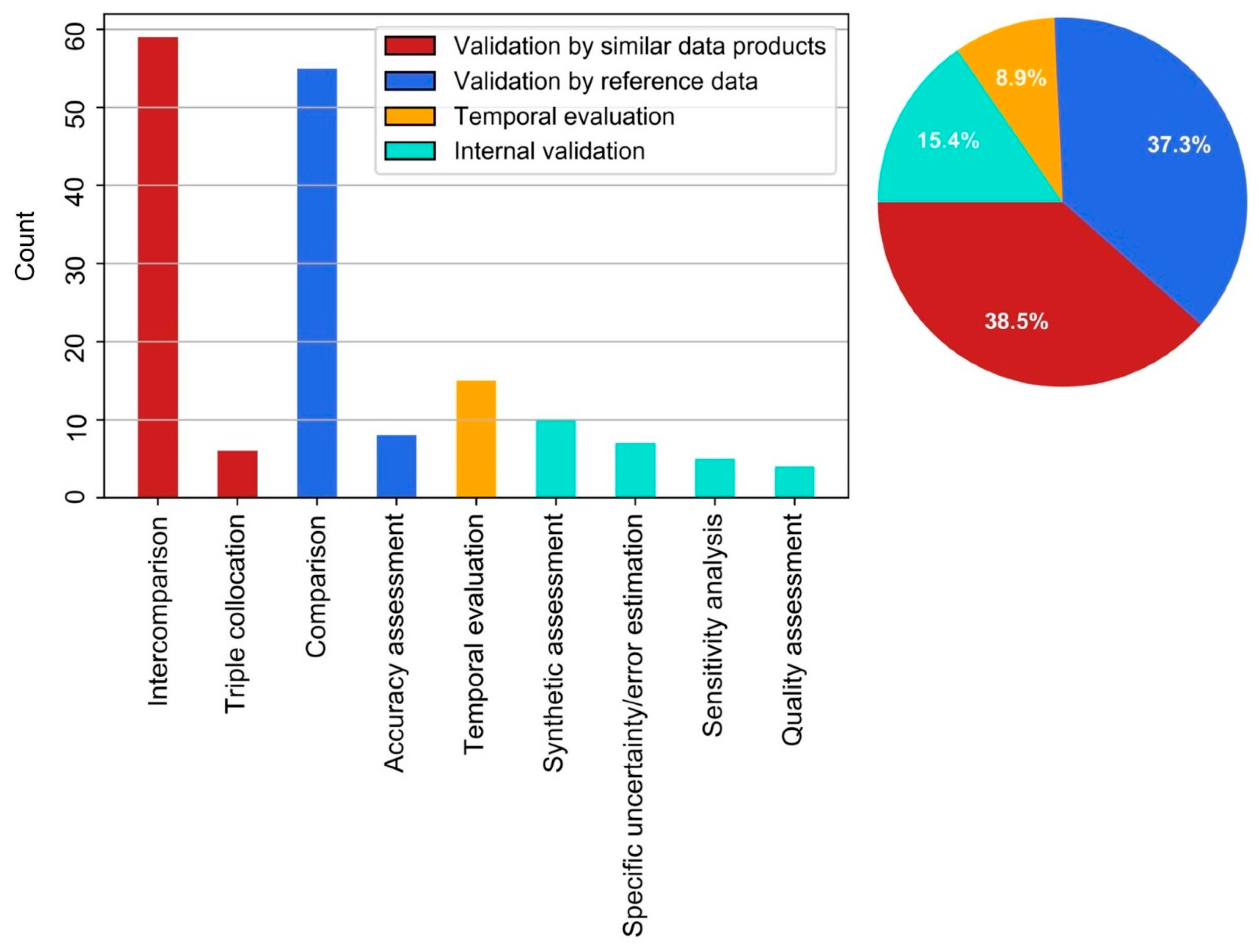
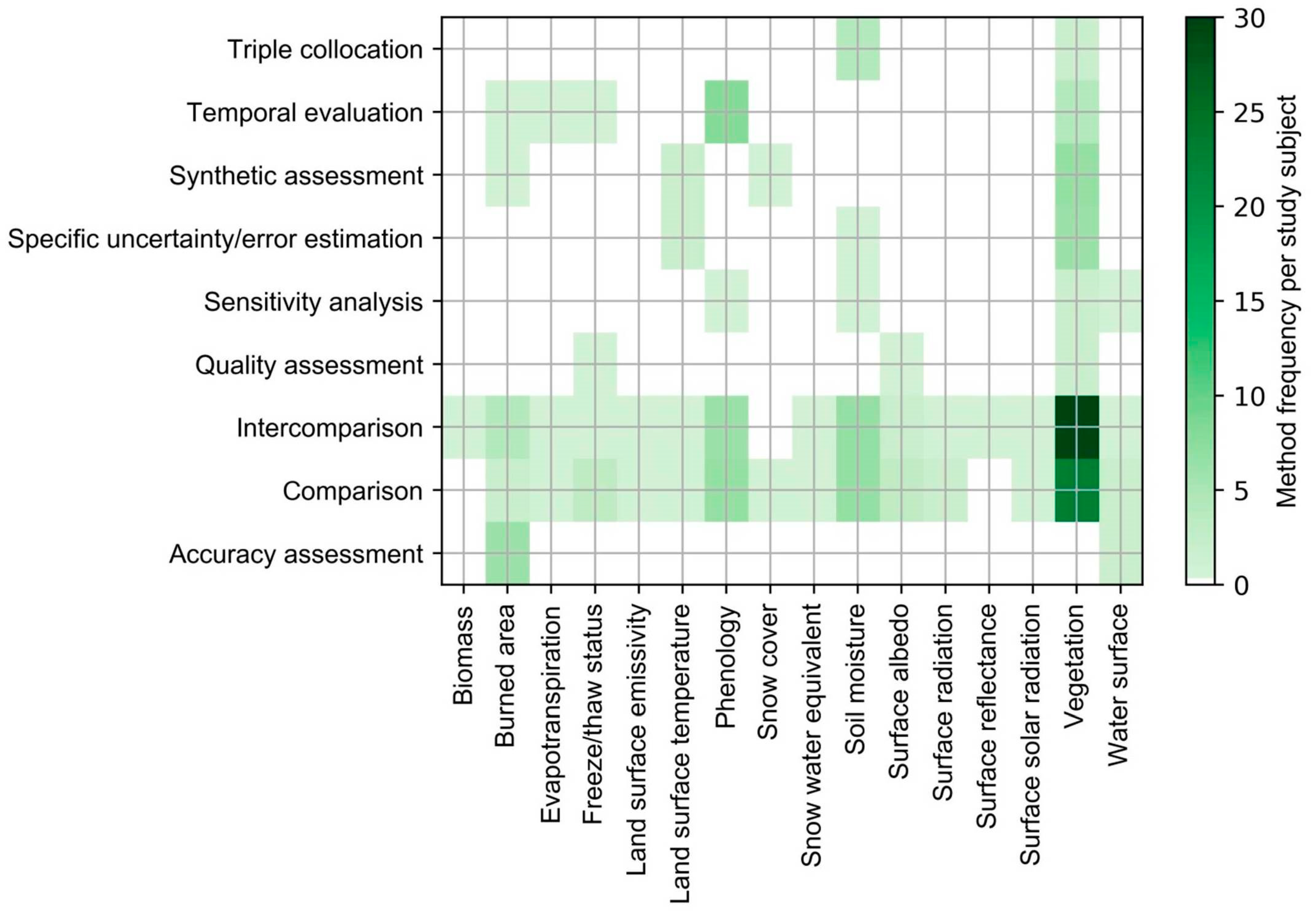
• The most commonly used validation method is the intercomparison of products (indirect validation, 38.5%), followed by the comparison to reference data (direct validation, 37.3%). The majority of studies used more than one validation method (65.9%).
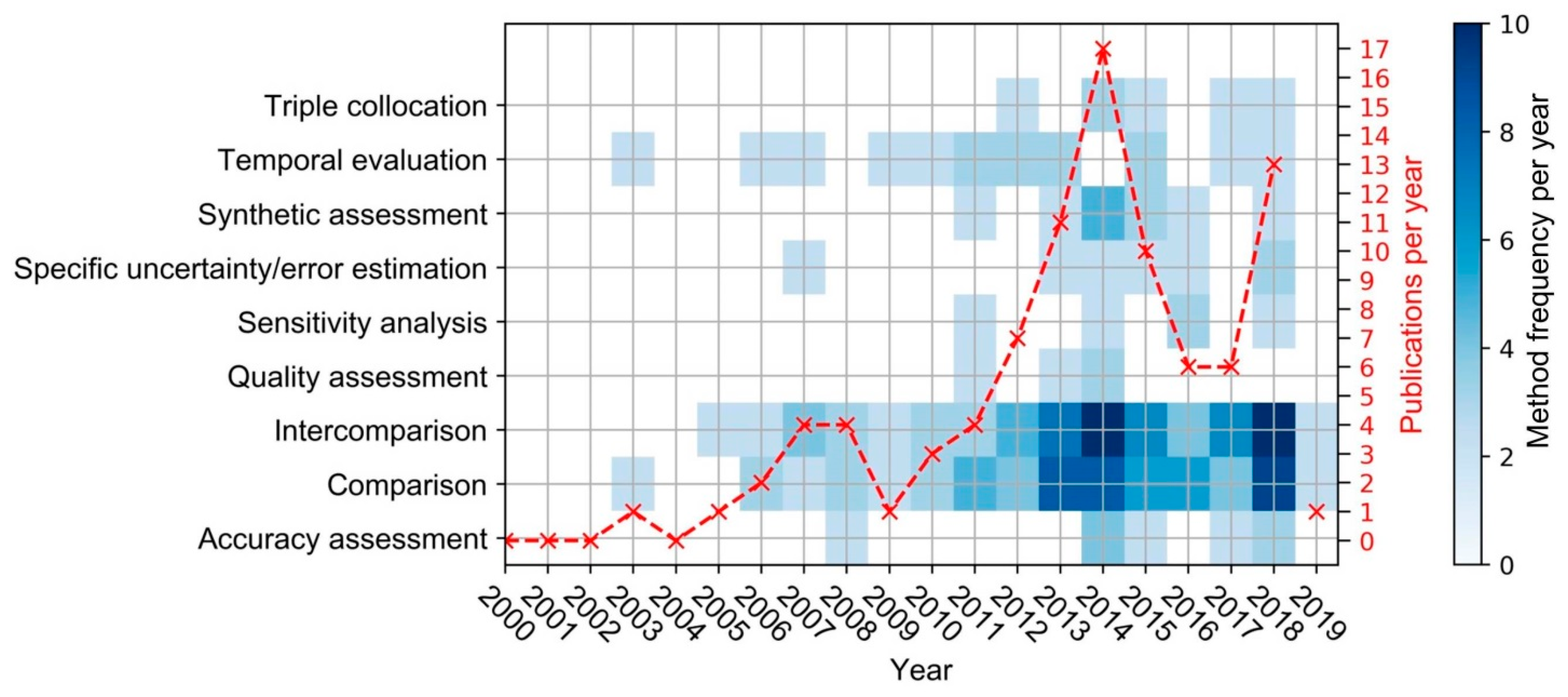
• A general increase in relevant studies published per year, along with a minor diversification of the corresponding validation methods, could be observed.
• Challenges comprise a lack of adequate reference data, consequently promoting other methods.
• The issue of matching product and validation data in a reasonable spatiotemporal fashion is seen throughout studies that consider external sources for validation.
• The use of validation methods that are not bound to external validation data is limited (15.4%), as is validation by time-series-derived points in time in temporal evaluations (8.9%).
• Validation by accuracy assessment is unfavored by the majority of studies in the scope of this review (4.7%), which excludes land use/land cover products.
• Although the assessment of physical uncertainty referring to the true state of a measured variable (direct validation) is demanded by major EO-related organizations, indirect validation is frequently implemented.

For long-term and large-area investigations, remote sensing offers unique advantages. A major constraining issue, however, is the need for reliable validation incorporating adequate validation data. Challenges and potential arise for the integration of remote sensing and ground observations [83], facilitating the application of traditional validation methods. To resolve the central issue of the lack of adequate reference data, new sources of validation data (e.g., near-surface remote sensing camera-bound vegetation indices [153], citizen science data [155,156]) could be considered. So far, one strategy is going towards the standardization of validation by the introduction of validation level hierarchies and observation requirements for measurement uncertainty for atmosphere-, land-, and ocean-related variables [2,32]. The hereby implied guidelines include the consistent use of reference data for validation. This development is sustained by extensive calibration and validations networks, providing reliable reference data in high spatiotemporal resolution. With progressive capabilities in the acquisition of EO data (e.g., Cubesat [157]), such networks could become even more relevant.

On the other hand, increasingly more applications of remote sensing data in sophisticated modelling efforts require auxiliary uncertainty estimations along with the product in high spatial and temporal resolution. Conventional validation methods that are based on reference data and even product intercomparisons are not able to properly fulfill this requirement. Also, differences in absolute values and inconsistencies in uncertainty representation still render some datasets inadequate for modelling or data fusion (e.g., FAPAR products [21]). A greater focus might be given to innovative internal methods, able to provide uncertainty information on the spot. With advances in novel techniques, this could be achieved in an automated fashion at the product generation stage, similar to the production of QC information. Some studies in the scope of this review have demonstrated approaches in line with this concept. However, publications that exhibit novel validation techniques are more typical for investigations of smaller regions of interest, facilitated in the development stage of a product (e.g., [158]). Nevertheless, internal methods have the potential to remedy the issue of the complete coverage of results with uncertainty information in space and time but are not able to provide uncertainty measures that are referenced to the true state of a geophysical variable. Consequently, this conception is missing physical uncertainties from a direct validation approach. A compromise could be achieved by strategies of rigorous validation by reference data in the development phase of a product and subsequent internal validation when the product is used in downstream applications that require more concise spatiotemporal quality information. Further research is needed to evaluate the capabilities and potential of novel methods, along with more extensive validation work in general to improve the understanding of remote sensing results, clearing the path for continuous high-quality data products.

References

1. Steffen, W.; Sanderson, R.A.; Tyson, P.D.; Jäger, J.; Matson, P.A.; Moore III, B.; Oldfield, F.; Richardson, K.; Schellnhuber, H.-J.; Turner, B.L.; et al. Global Change and the Earth System; Global Change—The IGBP Series; 2004; Springer: Berlin/Heidelberg, Germany, 2005; ISBN 91-631-5380-7. [Google Scholar]
2. GCOS (Global Climate Observing System). Essential Climate Variables, Monitoring Principles and Observation Requirements for Essential Land Climate Variables 2019. Available online: https://gcos.wmo.int/en/essential-climate-variables/gcos-monitoring-principles (accessed on 22 June 2019).
3. Metz, M.; Rocchini, D.; Neteler, M. Surface Temperatures at the Continental Scale. Remote Sens. 2014, 6, 3822–3840. [Google Scholar] [CrossRef]
4. Pereira, H.M.; Ferrier, S.; Walters, M.; Geller, G.N.; Jongman, R.H.G.; Scholes, R.J.; Bruford, M.W.; Brummitt, N.; Butchart, S.H.M.; Cardoso, A.C.; et al. Essential Biodiversity Variables. Science 2013, 339, 277–278. [Google Scholar] [CrossRef] [Green Version]
5. Yang, J.; Gong, P.; Fu, R.; Zhang, M.; Chen, J.; Liang, S.; Xu, B.; Shi, J.; Dickinson, R. The role of satellite remote sensing in climate change studies. Nat. Clim. Chang. 2013, 3, 875–883. [Google Scholar] [CrossRef]
6. Liang, S.; Zhao, X.; Liu, S.; Yuan, W.; Cheng, X.; Xiao, Z.; Zhang, X.; Liu, Q.; Cheng, J.; Tang, H.; et al. A long-term Global LAnd Surface Satellite (GLASS) data-set for environmental studies. Int. J. Digit. Earth 2013, 6, 5–33. [Google Scholar] [CrossRef]
7. Hay, S.I.; Tatem, A.J.; Graham, A.J.; Goetz, S.J.; Rogers, D.J. Global Environmental Data for Mapping Infectious Disease Distribution. In Global Mapping of Infectious Diseases: Methods, Examples and Emerging Applications; Advances in Parasitology; Elsevier: Amsterdam, The Netherlands, 2006; Volume 62, pp. 37–77. ISBN 978-0-12-031762-2. [Google Scholar]
8. Justice, C.; Belward, A.; Morisette, J.; Lewis, P.; Privette, J.; Baret, F. Developments in the “validation” of satellite sensor products for the study of the land surface. Int. J. Remote Sens. 2000, 21, 3383–3390. [Google Scholar] [CrossRef]
9. Weiss, M.; Baret, F.; Block, T.; Koetz, B.; Burini, A.; Scholze, B.; Lecharpentier, P.; Brockmann, C.; Fernandes, R.; Plummer, S.; et al. On Line Validation Exercise (OLIVE). Remote Sens. 2014, 6, 4190–4216. [Google Scholar] [CrossRef]
10. Kuenzer, C.; Dech, S.; Wagner, W. Remote Sensing Time Series; Springer International Publishing: Cham, Switzerland, 2015; Volume 22. [Google Scholar]
11. National Research Council. Climate Data Records from Environmental Satellites: Interim Report; The National Academies Press: Washington, DC, USA, 2004; ISBN 978-0-309-09168-8. [Google Scholar]
12. Kuenzer, C.; Ottinger, M.; Wegmann, M.; Guo, H.; Wang, C.; Zhang, J.; Dech, S.; Wikelski, M. Earth observation satellite sensors for biodiversity monitoring. Int. J. Remote Sens. 2014, 35, 6599–6647. [Google Scholar] [CrossRef]
13. MODIS Science Team 2019. Available online: https://modis.gsfc.nasa.gov/sci_team/ (accessed on 11 July 2019).
14. CGLS Copernicus Global Land Service. Available online: https://land.copernicus.eu/global/ (accessed on 2 September 2019).
15. Klein, C.; Bliefernicht, J.; Heinzeller, D.; Gessner, U.; Klein, I.; Kunstmann, H. Feedback of observed interannual vegetation change. Clim. Dyn. 2017, 48, 2837–2858. [Google Scholar] [CrossRef]
16. Machwitz, M.; Gessner, U.; Conrad, C.; Falk, U.; Richters, J.; Dech, S. Modelling the Gross Primary Productivity of West Africa with the Regional Biomass Model RBM+, using optimized 250 m MODIS FPAR and fractional vegetation cover information. Int. J. Appl. Earth Obs. Geoinf. 2015, 43, 177–194. [Google Scholar] [CrossRef]
17. Merkuryeva, G.; Merkuryev, Y.; Sokolov, B.V.; Potryasaev, S.; Zelentsov, V.A.; Lektauers, A. Advanced river flood monitoring, modelling and forecasting. J. Comput. Sci. 2015, 10, 77–85. [Google Scholar] [CrossRef]
18. Wißkirchen, K.; Tum, M.; Günther, K.P.; Niklaus, M.; Eisfelder, C.; Knorr, W. Quantifying the carbon uptake by vegetation for Europe on a 1 km2 resolution using a remote sensing driven vegetation model. Geosci. Model Dev. 2013, 6, 1623–1640. [Google Scholar] [CrossRef]
19. Döll, P.; Douville, H.; Güntner, A.; Müller Schmied, H.; Wada, Y. Modelling Freshwater Resources at the Global Scale. Surv. Geophys. 2016, 37, 195–221. [Google Scholar] [CrossRef]
20. Glenn, E.P.; Nagler, P.L.; Huete, A.R. Vegetation Index Methods for Estimating Evapotranspiration by Remote Sensing. Surv. Geophys. 2010, 31, 531–555. [Google Scholar] [CrossRef]
21. D’Odorico, P.; Gonsamo, A.; Pinty, B.; Gobron, N.; Coops, N.; Mendez, E.; Schaepman, M.E. Intercomparison of fraction of absorbed photosynthetically active radiation products derived from satellite data over Europe. Remote Sens. Environ. 2014, 142, 141–154. [Google Scholar] [CrossRef]
22. Fensholt, R.; Proud, S.R. Evaluation of Earth Observation based global long term vegetation trends—Comparing GIMMS and MODIS global NDVI time series. Remote Sens. Environ. 2012, 119, 131–147. [Google Scholar] [CrossRef]
23. Guay, K.C.; Beck, P.S.A.; Berner, L.T.; Goetz, S.J.; Baccini, A.; Buermann, W. Vegetation productivity patterns at high northern latitudes. Glob. Chang. Biol. 2014, 20, 3147–3158. [Google Scholar] [CrossRef]
24. Jiang, N.; Zhu, W.; Zheng, Z.; Chen, G.; Fan, D. A Comparative Analysis between GIMSS NDVIg and NDVI3g for Monitoring Vegetation Activity Change in the Northern Hemisphere during 1982–2008. Remote Sens. 2013, 5, 4031–4044. [Google Scholar] [CrossRef]
25. McCallum, I.; Wagner, W.; Schmullius, C.; Shvidenko, A.; Obersteiner, M.; Fritz, S.; Nilsson, S. Comparison of four global FAPAR datasets over Northern Eurasia for the year 2000. Remote Sens. Environ. 2010, 114, 941–949. [Google Scholar] [CrossRef]
26. Scheftic, W.; Zeng, X.; Broxton, P.; Brunke, M. Intercomparison of Seven NDVI Products over the United States and Mexico. Remote Sens. 2014, 6, 1057–1084. [Google Scholar] [CrossRef] [Green Version]
27. Wang, D.; Morton, D.; Masek, J.; Wu, A.; Nagol, J.; Xiong, X.; Levy, R.; Vermote, E.; Wolfe, R. Impact of sensor degradation on the MODIS NDVI time series. Remote Sens. Environ. 2012, 119, 55–61. [Google Scholar] [CrossRef] [Green Version]
28. Weiss, D.J.; Atkinson, P.M.; Bhatt, S.; Mappin, B.; Hay, S.I.; Gething, P.W. An effective approach for gap-filling continental scale remotely sensed time-series. ISPRS J. Photogramm. Remote Sens. Off. Publ. Int. Soc. Photogramm. Remote Sens. (ISPRS) 2014, 98, 106–118. [Google Scholar] [CrossRef] [PubMed] [Green Version]
29. Zhang, Y.; Song, C.; Band, L.E.; Sun, G.; Li, J. Reanalysis of global terrestrial vegetation trends from MODIS products. Remote Sens. Environ. 2017, 191, 145–155. [Google Scholar] [CrossRef]
30. Crosetto, M.; Tarantola, S. Uncertainty and sensitivity analysis: Tools for GIS-based model implementation. Int. J. Geogr. Inf. Sci. 2001, 15, 415–437. [Google Scholar] [CrossRef]
31. WMO (World Meteorological Organization). User Requirements for Observation 2019. Available online: http://www.wmo-sat.info/oscar/observingrequirements (accessed on 16 July 2019).
32. LPV (Land Product Validation). Subgroup CEOS Validation Hierarchy 2019. Available online: https://lpvs.gsfc.nasa.gov/ (accessed on 5 May 2019).
33. Salminen, M.; Pulliainen, J.; Metsämäki, S.; Ikonen, J.; Heinilä, K.; Luojus, K. Determination of uncertainty characteristics for the satellite data-based estimation of fractional snow cover. Remote Sens. Environ. 2018, 212, 103–113. [Google Scholar] [CrossRef]
34. Baret, F.; Weiss, M.; Lacaze, R.; Camacho, F.; Makhmara, H.; Pacholcyzk, P.; Smets, B. GEOV1: LAI and FAPAR essential climate variables and FCOVER global time series capitalizing over existing products. Part1: Principles of development and production. Remote Sens. Environ. 2013, 137, 299–309. [Google Scholar] [CrossRef]
35. Camacho, F.; Cernicharo, J.; Lacaze, R.; Baret, F.; Weiss, M. GEOV1: LAI, FAPAR essential climate variables and FCOVER global time series capitalizing over existing products. Part 2: Validation and intercomparison with reference products. Remote Sens. Environ. 2013, 137, 310–329. [Google Scholar] [CrossRef]
36. Klotz, M.; Kemper, T.; Geiß, C.; Esch, T.; Taubenböck, H. How good is the map? Remote Sens. Environ. 2016, 178, 191–212. [Google Scholar] [CrossRef]
37. Estes, L.; Chen, P.; Debats, S.; Evans, T.; Ferreira, S.; Kuemmerle, T.; Ragazzo, G.; Sheffield, J.; Wolf, A.; Wood, E.; et al. A large-area, spatially continuous assessment of land cover map error and its impact on downstream analyses. Glob. Chang. Biol. 2018, 24, 322–337. [Google Scholar] [CrossRef]
38. Congalton, R.G. A review of assessing the accuracy of classifications of remotely sensed data. Remote Sens. Environ. 1991, 37, 35–46. [Google Scholar] [CrossRef]
39. García-Haro, F.J.; Campos-Taberner, M.; Muñoz-Marí, J.; Laparra, V.; Camacho, F.; Sánchez-Zapero, J.; Camps-Valls, G. Derivation of global vegetation biophysical parameters from EUMETSAT Polar System. ISPRS J. Photogramm. Remote Sens. 2018, 139, 57–74. [Google Scholar] [CrossRef]
40. Olofsson, P.; Foody, G.M.; Herold, M.; Stehman, S.V.; Woodcock, C.E.; Wulder, M.A. Good practices for estimating area and assessing accuracy of land change. Remote Sens. Environ. 2014, 148, 42–57. [Google Scholar] [CrossRef]
41. Jansen, L.; Di Gregorio, A. Land Cover Classification System (LCCS); 2000; Food and Agriculture Organization of the United Nations: Rome, Italy, 1998. [Google Scholar]
42. Congalton, R.; Gu, J.; Yadav, K.; Thenkabail, P.; Ozdogan, M. Global Land Cover Mapping. Remote Sens. 2014, 6, 12070–12093. [Google Scholar] [CrossRef]
43. Strahler, A.H.; Boschetti, L.; Foody, G.M.; Friedl, M.A.; Hansen, M.C.; Herold, M.; Mayaux, P.; Morisette, J.; Stehman, S.; Woodcock, C. Global Land Cover Validation: Recommendations for Evaluation and Accuracy Assessment of Global Land Cover Maps; Office for Official Publications of the European Communities: Luxemburg, 2006; Volume 25. [Google Scholar]
44. Stehman, S.V.; Foody, G.M. Key issues in rigorous accuracy assessment of land cover products. Remote Sens. Environ. 2019, 231, 111199. [Google Scholar] [CrossRef]
45. Congalton, R.G.; Green, K. Assessing the Accuracy of Remotely Sensed Data: Principles and Practices, 2nd ed.; CRC Press/Taylor & Francis: Boca Raton, FL, USA, 2009; ISBN 978-1-4200-5512-2. [Google Scholar]
46. CEOS WGCV (Committee on Earth Observation Satellites Working Group on Calibration & Validation) 2019. Available online: http://ceos.org/ourwork/workinggroups/wgcv/ (accessed on 15 July 2019).
47. ISO (International Organization for Standardization). Accuracy (Trueness and Precision) of Measurement Methods and Results 1994. Available online: https://www.iso.org/obp/ui/#iso:std:iso:5725:-1:ed-1:v1:en (accessed on 15 July 2019).
48. Verger, A.; Baret, F.; Weiss, M. A multisensor fusion approach to improve LAI time series. Remote Sens. Environ. 2011, 115, 2460–2470. [Google Scholar] [CrossRef] [Green Version]
49. AIAA G-077. Guide for the Verification and Validation of Computational Fluid Dynamics Simulations; American Institute of Aeronautics and Astronautics: Reston, VA, USA, 1998; ISBN 978-1-56347-285-5. [Google Scholar]
50. Fisher, P.F. Models of uncertainty in spatial data. Geogr. Inf. Syst. 1999, 1, 191–205. [Google Scholar]
51. Demaria, E.M.C.; Serrat-Capdevila, A. Challenges of Remote Sensing Validation. In Earth Observation for Water Resources Management: Current Use and Future Opportunities for the Water Sector; The World Bank: Washington, DC, USA, 2016; pp. 167–171. ISBN 978-1-4648-0475-5. [Google Scholar]
52. Cao, C.; Xiong, X.; Wu, A.; Wu, X. Assessing the consistency of AVHRR and MODIS L1B reflectance for generating Fundamental Climate Data Records. J. Geophys. Res. 2008, 113, 33463. [Google Scholar] [CrossRef]
53. Weiss, M.; Baret, F.; Garrigues, S.; Lacaze, R. LAI and fAPAR CYCLOPES global products derived from VEGETATION. Part 2: Validation and comparison with MODIS collection 4 products. Remote Sens. Environ. 2007, 110, 317–331. [Google Scholar] [CrossRef]
54. Urban, M.; Eberle, J.; Hüttich, C.; Schmullius, C.; Herold, M. Comparison of Satellite-Derived Land Surface Temperature and Air Temperature from Meteorological Stations on the Pan-Arctic Scale. Remote Sens. 2013, 5, 2348–2367. [Google Scholar] [CrossRef] [Green Version]
55. Lei, F.; Crow, W.T.; Shen, H.; Su, C.-H.; Holmes, T.R.H.; Parinussa, R.M.; Wang, G. Assessment of the impact of spatial heterogeneity on microwave satellite soil moisture periodic error. Remote Sens. Environ. 2018, 205, 85–99. [Google Scholar] [CrossRef]
56. Widlowski, J.-L.; Taberner, M.; Pinty, B.; Bruniquel-Pinel, V.; Disney, M.; Fernandes, R.; Gastellu-Etchegorry, J.-P.; Gobron, N.; Kuusk, A.; Lavergne, T.; et al. Third Radiation Transfer Model Intercomparison (RAMI) exercise. J. Geophys. Res. 2007, 112, 1512. [Google Scholar] [CrossRef]
57. Wang, D.; Liang, S. Improving LAI Mapping by Integrating MODIS and CYCLOPES LAI Products Using Optimal Interpolation. IEEE J. Sel. Top. Appl. Earth Obs. Remote Sens. 2014, 7, 445–457. [Google Scholar] [CrossRef]
58. Zhou, J.; Jia, L.; Menenti, M.; Gorte, B. On the performance of remote sensing time series reconstruction methods—A spatial comparison. Remote Sens. Environ. 2016, 187, 367–384. [Google Scholar] [CrossRef]
59. Brown, M.E.; Pinzon, J.E.; Didan, K.; Morisette, J.T.; Tucker, C.J. Evaluation of the consistency of long-term NDVI time series derived from AVHRR, SPOT-vegetation, SeaWiFS, MODIS, and Landsat ETM+ sensors. IEEE Trans. Geosci. Remote Sens. 2006, 44, 1787–1793. [Google Scholar] [CrossRef]
60. Dorigo, W.A.; Xaver, A.; Vreugdenhil, M.; Gruber, A.; Hegyiová, A.; Sanchis-Dufau, A.D.; Zamojski, D.; Cordes, C.; Wagner, W.; Drusch, M. Global Automated Quality Control of In Situ Soil Moisture Data from the International Soil Moisture Network. Vadose Zone J. 2013, 12. [Google Scholar] [CrossRef]
61. Campbell, J.B. Introduction to Remote Sensing, 3rd ed.; Guilford Press: New York, NY, USA, 2002; ISBN 1-57230-640-8. [Google Scholar]
62. Myneni, R.B.; Ramakrishna, R.; Nemani, R.; Running, S.W. Estimation of global leaf area index and absorbed par using radiative transfer models. IEEE Trans. Geosci. Remote Sens. 1997, 35, 1380–1393. [Google Scholar] [CrossRef] [Green Version]
63. Padilla, M.; Stehman, S.; Litago, J.; Chuvieco, E. Assessing the Temporal Stability of the Accuracy of a Time Series of Burned Area Products. Remote Sens. 2014, 6, 2050–2068. [Google Scholar] [CrossRef] [Green Version]
64. Fang, H.; Wei, S.; Jiang, C.; Scipal, K. Theoretical uncertainty analysis of global MODIS, CYCLOPES, and GLOBCARBON LAI products using a triple collocation method. Remote Sens. Environ. 2012, 124, 610–621. [Google Scholar] [CrossRef]
65. Morisette, J.T.; Baret, F.; Privette, J.L.; Myneni, R.B.; Nickeson, J.E.; Garrigues, S.; Shabanov, N.V.; Weiss, M.; Fernandes, R.A.; Leblanc, S.G.; et al. Validation of global moderate-resolution LAI products. IEEE Trans. Geosci. Remote Sens. 2006, 44, 1804–1817. [Google Scholar] [CrossRef]
66. Ge, Y.; Li, X.; Hu, M.G.; Wang, J.H.; Jin, R.; Wang, J.F.; Zhang, R.H. Technical Specifications for the Validation of Remote Sensing Products. Int. Arch. Photogramm. Remote Sens. Spat. Inf. Sci. 2013, XL-2/W1, 13–17. [Google Scholar] [CrossRef]
67. McColl, K.A.; Vogelzang, J.; Konings, A.G.; Entekhabi, D.; Piles, M.; Stoffelen, A. Extended triple collocation: Estimating errors and correlation coefficients with respect to an unknown target: EXTENDED TRIPLE COLLOCATION. Geophys. Res. Lett. 2014, 41, 6229–6236. [Google Scholar] [CrossRef]
68. Soto-Berelov, M.; Jones, S.; Farmer, E.; Woodgate, W. Review of Validation Standards of Earth Observation Derived Biophysical Products, 11th ed.; Held, A., Phinn, S., Soto-Berelov, M., Jones, S., Eds.; TERN AusCover: Canberra, Australia, 2015. [Google Scholar]
69. Derksen, C.; Walker, A.; Goodison, B. A comparison of 18 winter seasons of in situ and passive microwave-derived snow water equivalent estimates in Western Canada. Remote Sens. Environ. 2003, 88, 271–282. [Google Scholar] [CrossRef]
70. Liang, S.; Fang, H.; Chen, M.; Shuey, C.J.; Walthall, C.; Daughtry, C.; Morisette, J.; Schaaf, C.; Strahler, A. Validating MODIS land surface reflectance and albedo products: Methods and preliminary results. Remote Sens. Environ. 2002, 83, 149–162. [Google Scholar] [CrossRef]
71. Xiao, Z.; Liang, S.; Wang, J.; Chen, P.; Yin, X.; Zhang, L.; Song, J. Use of General Regression Neural Networks for Generating the GLASS Leaf Area Index Product From Time-Series MODIS Surface Reflectance. IEEE Trans. Geosci. Remote Sens. 2014, 52, 209–223. [Google Scholar] [CrossRef]
72. Weiss, M.; Baret, F.; Smith, G.J.; Jonckheere, I.; Coppin, P. Review of methods for in situ leaf area index (LAI) determination. Agric. For. Meteorol. 2004, 121, 37–53. [Google Scholar] [CrossRef]
73. Djamai, N.; Fernandes, R.; Weiss, M.; McNairn, H.; Goïta, K. Validation of the Sentinel Simplified Level 2 Product Prototype Processor (SL2P) for mapping cropland biophysical variables using Sentinel-2/MSI and Landsat-8/OLI data. Remote Sens. Environ. 2019, 225, 416–430. [Google Scholar] [CrossRef]
74. CEOS (Committee on Earth Observation Satellites). Cal/Val Portal Cal/Val Sites 2019. Available online: http://calvalportal.ceos.org/ (accessed on 16 July 2019).
75. Gerstl, S.A.W. Physics concepts of optical and radar reflectance signatures A summary review. Int. J. Remote Sens. 1990, 11, 1109–1117. [Google Scholar] [CrossRef]
76. Chuvieco, E.; Lizundia-Loiola, J.; Pettinari, M.L.; Ramo, R.; Padilla, M.; Tansey, K.; Mouillot, F.; Laurent, P.; Storm, T.; Heil, A.; et al. Generation and analysis of a new global burned area product based on MODIS 250 m reflectance bands and thermal anomalies. Earth Syst. Sci. Data 2018, 10, 2015–2031. [Google Scholar] [CrossRef]
77. Higuchi, A.; Hiyama, T.; Fukuta, Y.; Suzuki, R.; Fukushima, Y. The behaviour of a surface temperature/vegetation index (TVX) matrix derived from 10-day composite AVHRR images over monsoon Asia. Hydrol. Process. 2007, 21, 1157–1166. [Google Scholar] [CrossRef]
78. Jones, M.O.; Jones, L.A.; Kimball, J.S.; McDonald, K.C. Satellite passive microwave remote sensing for monitoring global land surface phenology. Remote Sens. Environ. 2011, 115, 1102–1114. [Google Scholar] [CrossRef]
79. Rodell, M.; Chao, B.F.; Au, A.Y.; Kimball, J.S.; McDonald, K.C. Global Biomass Variation and Its Geodynamic Effects. Earth Interact. 2005, 9, 1–19. [Google Scholar] [CrossRef]
80. Huete, A.; Didan, K.; Miura, T.; Rodriguez, E.P.; Gao, X.; Ferreira, L.G. Overview of the radiometric and biophysical performance of the MODIS vegetation indices. Remote Sens. Environ. 2002, 83, 195–213. [Google Scholar] [CrossRef]
81. Cescatti, A.; Marcolla, B.; Santhana Vannan, S.K.; Pan, J.Y.; Román, M.O.; Yang, X.; Ciais, P.; Cook, R.B.; Law, B.E.; Matteucci, G.; et al. Intercomparison of MODIS albedo retrievals and in situ measurements across the global FLUXNET network. Remote Sens. Environ. 2012, 121, 323–334. [Google Scholar] [CrossRef] [Green Version]
82. Humber, M.L.; Boschetti, L.; Giglio, L.; Justice, C.O. Spatial and temporal intercomparison of four global burned area products. Int. J. Digit. Earth 2019, 12, 460–484. [Google Scholar] [CrossRef]
83. White, M.A.; Beurs, K.M.; Didan, K.; Inouye, D.W.; Richardson, A.D.; Jensen, O.P.; O’Keefe, J.; Zhang, G.; Nemani, R.R.; van Leeuwen, W.J.D.; et al. Intercomparison, interpretation, and assessment of spring phenology in North America estimated from remote sensing for 1982–2006. Glob. Chang. Biol. 2009, 15, 2335–2359. [Google Scholar] [CrossRef]
84. Jia, K.; Yang, L.; Liang, S.; Xiao, Z.; Zhao, X.; Yao, Y.; Zhang, X.; Jiang, B.; Liu, D. Long-Term Global Land Surface Satellite (GLASS) Fractional Vegetation Cover Product Derived From MODIS and AVHRR Data. IEEE J. Sel. Top. Appl. Earth Obs. Remote Sens. 2019, 12, 508–518. [Google Scholar] [CrossRef]
85. Ganguly, S.; Friedl, M.A.; Tan, B.; Zhang, X.; Verma, M. Land surface phenology from MODIS. Remote Sens. Environ. 2010, 114, 1805–1816. [Google Scholar] [CrossRef]
86. Pekel, J.-F.; Vancutsem, C.; Bastin, L.; Clerici, M.; Vanbogaert, E.; Bartholomé, E.; Defourny, P. A near real-time water surface detection method based on HSV transformation of MODIS multi-spectral time series data. Remote Sens. Environ. 2014, 140, 704–716. [Google Scholar] [CrossRef] [Green Version]
87. Gobron, N.; Pinty, B.; Mélin, F.; Taberner, M.; Verstraete, M.M.; Robustelli, M.; Widlowski, J.-L. Evaluation of the MERIS/ENVISAT FAPAR product. Adv. Space Res. 2007, 39, 105–115. [Google Scholar] [CrossRef]
88. Padilla, M.; Stehman, S.V.; Ramo, R.; Corti, D.; Hantson, S.; Oliva, P.; Alonso-Canas, I.; Bradley, A.V.; Tansey, K.; Mota, B.; et al. Comparing the accuracies of remote sensing global burned area products using stratified random sampling and estimation. Remote Sens. Environ. 2015, 160, 114–121. [Google Scholar] [CrossRef] [Green Version]
89. Potter, C.; Tan, P.-N.; Steinbach, M.; Klooster, S.; Kumar, V.; Myneni, R.; Genovese, V. Major disturbance events in terrestrial ecosystems detected using global satellite data sets. Glob. Chang. Biol. 2003, 9, 1005–1021. [Google Scholar] [CrossRef] [Green Version]
90. Ramo, R.; García, M.; Rodríguez, D.; Chuvieco, E. A data mining approach for global burned area mapping. Int. J. Appl. Earth Obs. Geoinf. 2018, 73, 39–51. [Google Scholar] [CrossRef]
91. Zhang, X.; Zhang, Q. Monitoring interannual variation in global crop yield using long-term AVHRR and MODIS observations. ISPRS J. Photogramm. Remote Sens. 2016, 114, 191–205. [Google Scholar] [CrossRef]
92. Chen, F.; Crow, W.T.; Colliander, A.; Cosh, M.H.; Jackson, T.J.; Bindlish, R.; Reichle, R.H.; Chan, S.K.; Bosch, D.D.; Starks, P.J.; et al. Application of Triple Collocation in Ground-Based Validation of Soil Moisture Active/Passive (SMAP) Level 2 Data Products. IEEE J. Sel. Top. Appl. Earth Obs. Remote Sens. 2017, 10, 489–502. [Google Scholar] [CrossRef]
93. Chen, F.; Crow, W.T.; Bindlish, R.; Colliander, A.; Burgin, M.S.; Asanuma, J.; Aida, K. Global-scale evaluation of SMAP, SMOS and ASCAT soil moisture products using triple collocation. Remote Sens. Environ. 2018, 214, 1–13. [Google Scholar] [CrossRef]
94. Fang, H.; Liang, S.; Townshend, J.; Dickinson, R. Spatially and temporally continuous LAI data sets based on an integrated filtering method. Remote Sens. Environ. 2008, 112, 75–93. [Google Scholar] [CrossRef]
95. Marshall, M.; Okuto, E.; Kang, Y.; Opiyo, E.; Ahmed, M. Global assessment of Vegetation Index and Phenology Lab (VIP) and Global Inventory Modeling and Mapping Studies (GIMMS) version 3 products. Biogeosciences 2016, 13, 625–639. [Google Scholar] [CrossRef] [Green Version]
96. Xiao, Z.; Liang, S.; Sun, R. Evaluation of Three Long Time Series for Global Fraction of Absorbed Photosynthetically Active Radiation (FAPAR) Products. IEEE Trans. Geosci. Remote Sens. 2018, 56, 5509–5524. [Google Scholar] [CrossRef]
97. Xiao, Z.; Liang, S.; Jiang, B. Evaluation of four long time-series global leaf area index products. Agric. For. Meteorol. 2017, 246, 218–230. [Google Scholar] [CrossRef]
98. Chuvieco, E.; Opazo, S.; Sione, W.; del Valle, H.; Anaya, J.; Di Bella, C.; Cruz, I.; Manzo, L.; López, G.; Mari, N.; et al. Global Burned Area Estimation in Latin America Using MODIS Composite Data. Ecol. Appl. 2008, 18, 64–79. [Google Scholar] [CrossRef]
99. Sobrino, J.A.; Julien, Y. Global trends in NDVI-derived parameters obtained from GIMMS data. Int. J. Remote Sens. 2011, 32, 4267–4279. [Google Scholar] [CrossRef]
100. Tarnavsky, E.; Garrigues, S.; Brown, M.E. Multiscale geostatistical analysis of AVHRR, SPOT-VGT, and MODIS global NDVI products. Remote Sens. Environ. 2008, 112, 535–549. [Google Scholar] [CrossRef]
101. Kandasamy, S.; Baret, F.; Verger, A.; Neveux, P.; Weiss, M. A comparison of methods for smoothing and gap filling time series of remote sensing observations—Application to MODIS LAI products. Biogeosciences 2013, 10, 4055–4071. [Google Scholar] [CrossRef]
102. Schwartz, M.D.; Hanes, J.M. Intercomparing multiple measures of the onset of spring in eastern North America. Int. J. Climatol. 2010, 30, 1614–1626. [Google Scholar] [CrossRef]
103. Wang, Q.; Tenhunen, J.; Dinh, N.; Reichstein, M.; Otieno, D.; Granier, A.; Pilegarrd, K. Evaluation of seasonal variation of MODIS derived leaf area index at two European deciduous broadleaf forest sites. Remote Sens. Environ. 2005, 96, 475–484. [Google Scholar] [CrossRef]
104. Forkel, M.; Migliavacca, M.; Thonicke, K.; Reichstein, M.; Schaphoff, S.; Weber, U.; Carvalhais, N. Codominant water control on global interannual variability and trends in land surface phenology and greenness. Glob. Chang. Biol. 2015, 21, 3414–3435. [Google Scholar] [CrossRef]
105. Wu, C.; Peng, D.; Soudani, K.; Siebicke, L.; Gough, C.M.; Arain, M.A.; Bohrer, G.; Lafleur, P.M.; Peichl, M.; Gonsamo, A.; et al. Land surface phenology derived from normalized difference vegetation index (NDVI) at global FLUXNET sites. Agric. For. Meteorol. 2017, 233, 171–182. [Google Scholar] [CrossRef]
106. Gruber, A.; Su, C.-H.; Zwieback, S.; Crow, W.; Dorigo, W.; Wagner, W. Recent advances in (soil moisture) triple collocation analysis. Int. J. Appl. Earth Obs. Geoinf. 2016, 45, 200–211. [Google Scholar] [CrossRef]
107. Jones, M.O.; Kimball, J.S.; Jones, L.A.; McDonald, K.C. Satellite passive microwave detection of North America start of season. Remote Sens. Environ. 2012, 123, 324–333. [Google Scholar] [CrossRef]
108. Kim, Y.; Kimball, J.S.; McDonald, K.C.; Glassy, J. Developing a Global Data Record of Daily Landscape Freeze/Thaw Status Using Satellite Passive Microwave Remote Sensing. IEEE Trans. Geosci. Remote Sens. 2011, 49, 949–960. [Google Scholar] [CrossRef]
109. Papa, F.; Prigent, C.; Aires, F.; Jimenez, C.; Rossow, W.B.; Matthews, E. Interannual variability of surface water extent at the global scale, 1993–2004. J. Geophys. Res. 2010, 115, 1147. [Google Scholar] [CrossRef]
110. Zwieback, S.; Paulik, C.; Wagner, W. Frozen Soil Detection Based on Advanced Scatterometer Observations and Air Temperature Data as Part of Soil Moisture Retrieval. Remote Sens. 2015, 7, 3206–3231. [Google Scholar] [CrossRef] [Green Version]
111. Keersmaecker, W.; Lhermitte, S.; Honnay, O.; Farifteh, J.; Somers, B.; Coppin, P. How to measure ecosystem stability? An evaluation of the reliability of stability metrics based on remote sensing time series across the major global ecosystems. Glob. Chang. Biol. 2014, 20, 2149–2161. [Google Scholar] [CrossRef]
112. Al-Yaari, A.; Wigneron, J.-P.; Ducharne, A.; Kerr, Y.H.; Wagner, W.; Lannoy, G.; Reichle, R.; Al Bitar, A.; Dorigo, W.; Richaume, P.; et al. Global-scale comparison of passive (SMOS) and active (ASCAT) satellite based microwave soil moisture retrievals with soil moisture simulations (MERRA-Land). Remote Sens. Environ. 2014, 152, 614–626. [Google Scholar] [CrossRef] [Green Version]
113. Brown, M.E.; Lary, D.J.; Vrieling, A.; Stathakis, D.; Mussa, H. Neural networks as a tool for constructing continuous NDVI time series from AVHRR and MODIS. Int. J. Remote Sens. 2008, 29, 7141–7158. [Google Scholar] [CrossRef] [Green Version]
114. Bruscantini, C.A.; Konings, A.G.; Narvekar, P.S.; McColl, K.A.; Entekhabi, D.; Grings, F.M.; Karszenbaum, H. L-Band Radar Soil Moisture Retrieval Without Ancillary Information. IEEE J. Sel. Top. Appl. Earth Obs. Remote Sens. 2015, 8, 5526–5540. [Google Scholar] [CrossRef]
115. Cheng, J.; Liang, S.; Yao, Y.; Ren, B.; Shi, L.; Liu, H. A Comparative Study of Three Land Surface Broadband Emissivity Datasets from Satellite Data. Remote Sens. 2013, 6, 111–134. [Google Scholar] [CrossRef] [Green Version]
116. Fontana, F.M.A.; Coops, N.C.; Khlopenkov, K.V.; Trishchenko, A.P.; Riffler, M.; Wulder, M.A. Generation of a novel 1km NDVI data set over Canada, the northern United States, and Greenland based on historical AVHRR data. Remote Sens. Environ. 2012, 121, 171–185. [Google Scholar] [CrossRef]
117. Franch, B.; Vermote, E.; Roger, J.-C.; Murphy, E.; Becker-Reshef, I.; Justice, C.; Claverie, M.; Nagol, J.; Csiszar, I.; Meyer, D.; et al. A 30+ Year AVHRR Land Surface Reflectance Climate Data Record and Its Application to Wheat Yield Monitoring. Remote Sens. 2017, 9, 296. [Google Scholar] [CrossRef]
118. Kohler, P.; Guanter, L.; Frankenberg, C. Simplified physically based retrieval of sun-induced chlorophyll fluorescence from GOSAT data. IEEE Geosci. Remote Sens. Lett. 2015, 12, 1446–1450. [Google Scholar] [CrossRef]
119. Pan, N.; Feng, X.; Fu, B.; Wang, S.; Ji, F.; Pan, S. Increasing global vegetation browning hidden in overall vegetation greening: Insights from time-varying trends. Remote Sens. Environ. 2018, 214, 59–72. [Google Scholar] [CrossRef]
120. Bojanowski, J.S.; Vrieling, A.; Skidmore, A.K. A comparison of data sources for creating a long-term time series of daily gridded solar radiation for Europe. Sol. Energy 2014, 99, 152–171. [Google Scholar] [CrossRef]
121. Jia, A.; Liang, S.; Jiang, B.; Zhang, X.; Wang, G. Comprehensive Assessment of Global Surface Net Radiation Products and Uncertainty Analysis. J. Geophys. Res. Atmos. 2018, 123, 1970–1989. [Google Scholar] [CrossRef]
122. Piles, M.; Ballabrera-Poy, J.; Muñoz-Sabater, J. Dominant Features of Global Surface Soil Moisture Variability Observed by the SMOS Satellite. Remote Sens. 2019, 11, 95. [Google Scholar] [CrossRef]
123. Albergel, C.; Dorigo, W.; Reichle, R.H.; Balsamo, G.; Rosnay, P.; Muñoz-Sabater, J.; Isaksen, L.; Jeu, R.; Wagner, W. Skill and Global Trend Analysis of Soil Moisture from Reanalyses and Microwave Remote Sensing. J. Hydrometeorol. 2013, 14, 1259–1277. [Google Scholar] [CrossRef]
124. Gruber, A.; Dorigo, W.A.; Crow, W.; Wagner, W. Triple Collocation-Based Merging of Satellite Soil Moisture Retrievals. IEEE Trans. Geosci. Remote Sens. 2017, 55, 6780–6792. [Google Scholar] [CrossRef]
125. Suzuki, R.; Masuda, K.; Dye, D.G. Interannual covariability between actual evapotranspiration and PAL and GIMMS NDVIs of northern Asia. Remote Sens. Environ. 2007, 106, 387–398. [Google Scholar] [CrossRef]
126. Müller, R.; Pfeifroth, U.; Träger-Chatterjee, C.; Trentmann, J.; Cremer, R. Digging the METEOSAT Treasure—3 Decades of Solar Surface Radiation. Remote Sens. 2015, 7, 8067–8101. [Google Scholar] [CrossRef]
127. Munier, S.; Carrer, D.; Planque, C.; Camacho, F.; Albergel, C.; Calvet, J.-C. Satellite Leaf Area Index: Global Scale Analysis of the Tendencies Per Vegetation Type Over the Last 17 Years. Remote Sens. 2018, 10, 424. [Google Scholar] [CrossRef]
128. Paulik, C.; Dorigo, W.; Wagner, W.; Kidd, R. Validation of the ASCAT Soil Water Index using in situ data from the International Soil Moisture Network. Int. J. Appl. Earth Obs. Geoinf. 2014, 30, 1–8. [Google Scholar] [CrossRef]
129. Jia, K.; Liang, S.; Liu, S.; Li, Y.; Xiao, Z.; Yao, Y.; Jiang, B.; Zhao, X.; Wang, X.; Xu, S.; et al. Global Land Surface Fractional Vegetation Cover Estimation Using General Regression Neural Networks From MODIS Surface Reflectance. IEEE Trans. Geosci. Remote Sens. 2015, 53, 4787–4796. [Google Scholar] [CrossRef]
130. Padilla, M.; Stehman, S.V.; Chuvieco, E. Validation of the 2008 MODIS-MCD45 global burned area product using stratified random sampling. Remote Sens. Environ. 2014, 144, 187–196. [Google Scholar] [CrossRef]
131. Klein, I.; Gessner, U.; Dietz, A.J.; Kuenzer, C. Global WaterPack—A 250 m resolution dataset revealing the daily dynamics of global inland water bodies. Remote Sens. Environ. 2017, 198, 345–362. [Google Scholar] [CrossRef]
132. Dietz, A.J.; Kuenzer, C.; Dech, S. Global SnowPack. Remote Sens. Lett. 2015, 6, 844–853. [Google Scholar] [CrossRef]
133. Kim, Y.; Kimball, J.S.; Zhang, K.; McDonald, K.C. Satellite detection of increasing Northern Hemisphere non-frozen seasons from 1979 to 2008. Remote Sens. Environ. 2012, 121, 472–487. [Google Scholar] [CrossRef]
134. Zhang, X.; Friedl, M.A.; Schaaf, C.B. Global vegetation phenology from Moderate Resolution Imaging Spectroradiometer (MODIS): Evaluation of global patterns and comparison with in situ measurements. J. Geophys. Res. 2006, 111, G04017. [Google Scholar] [CrossRef]
135. Hu, G.; Jia, L.; Menenti, M. Comparison of MOD16 and LSA-SAF MSG evapotranspiration products over Europe for 2011. Remote Sens. Environ. 2015, 156, 510–526. [Google Scholar] [CrossRef]
136. Mu, X.; Song, W.; Gao, Z.; McVicar, T.R.; Donohue, R.J.; Yan, G. Fractional vegetation cover estimation by using multi-angle vegetation index. Remote Sens. Environ. 2018, 216, 44–56. [Google Scholar] [CrossRef]
137. Zhou, J.; Jia, L.; Menenti, M. Reconstruction of global MODIS NDVI time series. Remote Sens. Environ. 2015, 163, 217–228. [Google Scholar] [CrossRef]
138. Kumar, S.V.; Dirmeyer, P.A.; Peters-Lidard, C.D.; Bindlish, R.; Bolten, J. Information theoretic evaluation of satellite soil moisture retrievals. Remote Sens. Environ. 2018, 204, 392–400. [Google Scholar] [CrossRef]
139. Rodríguez-Fernández, N.; Kerr, Y.; van der Schalie, R.; Al-Yaari, A.; Wigneron, J.-P.; de Jeu, R.; Richaume, P.; Dutra, E.; Mialon, A.; Drusch, M. Long Term Global Surface Soil Moisture Fields Using an SMOS-Trained Neural Network Applied to AMSR-E Data. Remote Sens. 2016, 8, 959. [Google Scholar] [CrossRef]
140. Sichangi, A.W.; Wang, L.; Yang, K.; Chen, D.; Wang, Z.; Li, X.; Zhou, J.; Liu, W.; Kuria, D. Estimating continental river basin discharges using multiple remote sensing data sets. Remote Sens. Environ. 2016, 179, 36–53. [Google Scholar] [CrossRef] [Green Version]
141. Fang, H.; Wei, S.; Liang, S. Validation of MODIS and CYCLOPES LAI products using global field measurement data. Remote Sens. Environ. 2012, 119, 43–54. [Google Scholar] [CrossRef]
142. Liu, J.; Li, Z.; Huang, L.; Tian, B. Hemispheric-scale comparison of monthly passive microwave snow water equivalent products. J. Appl. Remote Sens. 2014, 8, 084688. [Google Scholar] [CrossRef]
143. Liu, Q.; Wang, L.; Qu, Y.; Liu, N.; Liu, S.; Tang, H.; Liang, S. Preliminary evaluation of the long-term GLASS albedo product. Int. J. Digit. Earth 2013, 6, 69–95. [Google Scholar] [CrossRef]
144. Tum, M.; Günther, K.; Böttcher, M.; Baret, F.; Bittner, M.; Brockmann, C.; Weiss, M. Global Gap-Free MERIS LAI Time Series (2002–2012). Remote Sens. 2016, 8, 69. [Google Scholar] [CrossRef]
145. Wu, D.; Wu, H.; Zhao, X.; Zhou, T.; Tang, B.; Zhao, W.; Jia, K. Evaluation of Spatiotemporal Variations of Global Fractional Vegetation Cover Based on GIMMS NDVI Data from 1982 to 2011. Remote Sens. 2014, 6, 4217–4239. [Google Scholar] [CrossRef] [Green Version]
146. Entekhabi, D.; Reichle, R.H.; Koster, R.D.; Crow, W.T. Performance Metrics for Soil Moisture Retrievals and Application Requirements. J. Hydrometeorol. 2010, 11, 832–840. [Google Scholar] [CrossRef]
147. Stanski, H.R.; Wilson, L.; Burrows, W. Survey of Common Verification Methods in Meteorology; World Meteorological Organisation: Geneva, Switzerland, 1990; Volume 8. [Google Scholar]
148. Janssen, P.A.E.M.; Abdalla, S.; Hersbach, H.; Bidlot, J.-R. Error Estimation of Buoy, Satellite, and Model Wave Height Data. J. Atmos. Ocean. Technol. 2007, 24, 1665–1677. [Google Scholar] [CrossRef] [Green Version]
149. Boschetti, L.; Roy, D.P.; Justice, C.O. International Global Burned Area Satellite Product Validation Protocol Part I—Production and Standardization of Validation Reference Data (to be Followed by Part II—Accuracy Reporting); Committee on Earth Observation Satellites: Maryland, MD, USA, 2009; pp. 1–11. [Google Scholar]
150. Baret, F.; Morissette, J.T.; Fernandes, R.A.; Champeaux, J.L.; Myneni, R.B.; Chen, J.; Plummer, S.; Weiss, M.; Bacour, C.; Garrigues, S.; et al. Evaluation of the representativeness of networks of sites for the global validation and intercomparison of land biophysical products: Proposition of the CEOS-BELMANIP. IEEE Trans. Geosci. Remote Sens. 2006, 44, 1794–1803. [Google Scholar] [CrossRef]
151. Garrigues, S.; Lacaze, R.; Baret, F.; Morisette, J.T.; Weiss, M.; Nickeson, J.E.; Fernandes, R.; Plummer, S.; Shabanov, N.V.; Myneni, R.B.; et al. Validation and intercomparison of global Leaf Area Index products derived from remote sensing data. J. Geophys. Res. 2008, 113. [Google Scholar] [CrossRef]
152. Tan, B.; Woodcock, C.E.; Hu, J.; Zhang, P.; Ozdogan, M.; Huang, D.; Yang, W.; Knyazikhin, Y.; Myneni, R.B. The impact of gridding artifacts on the local spatial properties of MODIS data: Implications for validation, compositing, and band-to-band registration across resolutions. Remote Sens. Environ. 2006, 105, 98–114. [Google Scholar] [CrossRef]
153. Hufkens, K.; Friedl, M.; Sonnentag, O.; Braswell, B.H.; Milliman, T.; Richardson, A.D. Linking near-surface and satellite remote sensing measurements of deciduous broadleaf forest phenology. Remote Sens. Environ. 2012, 117, 307–321. [Google Scholar] [CrossRef]
154. Verbesselt, J.; Hyndman, R.; Newnham, G.; Culvenor, D. Detecting trend and seasonal changes in satellite image time series. Remote Sens. Environ. 2010, 114, 106–115. [Google Scholar] [CrossRef]
155. See, L.; Mooney, P.; Foody, G.; Bastin, L.; Comber, A.; Estima, J.; Fritz, S.; Kerle, N.; Jiang, B.; Laakso, M.; et al. Crowdsourcing, Citizen Science or Volunteered Geographic Information? The Current State of Crowdsourced Geographic Information. IJGI Int. J. Geo Inf. 2016, 5, 55. [Google Scholar] [CrossRef]
156. Wulder, M.A.; Coops, N.C.; Roy, D.P.; White, J.C.; Hermosilla, T. Land cover 2.0. Int. J. Remote Sens. 2018, 39, 4254–4284. [Google Scholar] [CrossRef] [Green Version]
157. Houborg, R.; McCabe, M.F. A Cubesat enabled Spatio-Temporal Enhancement Method (CESTEM) utilizing Planet, Landsat and MODIS data. Remote Sens. Environ. 2018, 209, 211–226. [Google Scholar] [CrossRef]
158. Peter, B.G.; Messina, J.P. Errors in Time-Series Remote Sensing and an Open Access Application for Detecting and Visualizing Spatial Data Outliers Using Google Earth Engine. IEEE J. Sel. Top. Appl. Earth Obs. Remote Sens. 2019, 12, 1165–1174. [Google Scholar] [CrossRef]
Figure 1. Physical earth (top) and global Satellite Pour l’Observation de la Terre Vegetation (SPOTVGT) fraction of absorbed photosynthetically active radiation (FAPAR) product (center [34,35]) with ancillary accuracy information (bottom, source [14]).
Remotesensing 11 02616 g001
Figure 2. Journal histogram according to the paper selection in this review. Full journal names can be found in Table A1.
Remotesensing 11 02616 g002
Figure 3. Schematic illustration of validation terms shown for four stages of different measurement mean and variance. Green dots show measurements for every true state (black dots) and its vicinity (blue circles).
Remotesensing 11 02616 g003
Figure 4. Error sources and corresponding corrections in the generation of earth observation time-series.
Remotesensing 11 02616 g004
Figure 5. Sensors used for time-series generation in this review. Full sensor names can be found in Table A1.
Remotesensing 11 02616 g005
Figure 6. Utilization frequency of time-series-derived variables in the reviewed studies.
Remotesensing 11 02616 g006
Figure 7. Investigation periods and data sources of the reviewed studies. The coloring highlights the three most frequently utilized sensors as well as their combinations.
Remotesensing 11 02616 g007
Figure 8. Frequency of research objects in the reviewed studies and their affiliation to superordinate domains.
Remotesensing 11 02616 g008
Figure 9. The number of reviewed studies in specific regions of interest.
Remotesensing 11 02616 g009
Figure 10. Categorization of validation methods by the use of validation data.
Remotesensing 11 02616 g010
Figure 11. Validation data used in the studies grouped by source.
Remotesensing 11 02616 g011
Figure 12. The number of applied validation methods categorized by the validation data source.
Remotesensing 11 02616 g012
Figure 13. Frequency of the applied validation methods according to study subjects.
Remotesensing 11 02616 g013
Figure 14. Frequency of the concepts/metrics used for the expression of validation results in the reviewed studies.
Remotesensing 11 02616 g014
Figure 15. Temporal development of the number of relevant publications and application frequency of validation methods (trend to 2019 is not indicated).
Remotesensing 11 02616 g015