Article

A Comparative Study of RGB and Multispectral Sensor-Based Cotton Canopy Cover Modelling Using Multi-Temporal UAS Data

1
Lyles School of Civil Engineering, Purdue University, West Lafayette, IN 47907, USA
2
School of Engineering & Computing Science, Texas A&M University– Corpus Christi, Corpus Christi, TX 78412, USA
3
Texas A&M AgriLife Extension, Lubbock, TX 79403, USA
4
Texas A&M AgriLife Research, Corpus Christi, TX 78406, USA
*
Author to whom correspondence should be addressed.
Remote Sens. 2019, 11(23), 2757; https://0-doi-org.brum.beds.ac.uk/10.3390/rs11232757
Submission received: 22 October 2019 / Revised: 20 November 2019 / Accepted: 21 November 2019 / Published: 23 November 2019
(This article belongs to the Special Issue UAVs for Vegetation Monitoring)

Abstract

:
This study presents a comparative study of multispectral and RGB (red, green, and blue) sensor-based cotton canopy cover modelling using multi-temporal unmanned aircraft systems (UAS) imagery. Additionally, a canopy cover model using an RGB sensor is proposed that combines an RGB-based vegetation index with morphological closing. The field experiment was established in 2017 and 2018, where the whole study area was divided into approximately 1 x 1 m size grids. Grid-wise percentage canopy cover was computed using both RGB and multispectral sensors over multiple flights during the growing season of the cotton crop. Initially, the normalized difference vegetation index (NDVI)-based canopy cover was estimated, and this was used as a reference for the comparison with RGB-based canopy cover estimations. To test the maximum achievable performance of RGB-based canopy cover estimation, a pixel-wise classification method was implemented. Later, four RGB-based canopy cover estimation methods were implemented using RGB images, namely Canopeo, the excessive greenness index, the modified red green vegetation index and the red green blue vegetation index. The performance of RGB-based canopy cover estimation was evaluated using NDVI-based canopy cover estimation. The multispectral sensor-based canopy cover model was considered to be a more stable and accurately estimating canopy cover model, whereas the RGB-based canopy cover model was very unstable and failed to identify canopy when cotton leaves changed color after canopy maturation. The application of a morphological closing operation after the thresholding significantly improved the RGB-based canopy cover modeling. The red green blue vegetation index turned out to be the most efficient vegetation index to extract canopy cover with very low average root mean square error (2.94% for the 2017 dataset and 2.82% for the 2018 dataset), with respect to multispectral sensor-based canopy cover estimation. The proposed canopy cover model provides an affordable alternate of the multispectral sensors which are more sensitive and expensive.

Graphical Abstract

1. Introduction

Numerous studies are being conducted on cotton crop growth monitoring for precision agriculture. Cotton is an important crop in the state of Texas, which produces more than 50% of the total cotton produced by the entire country, comprising a spatial coverage of around six million acres [1]. Recent advances in genetic engineering and genomics have significantly accelerated the breeding process of cotton [2]. There is a growing need for phenotyping to match this high pace breeding process. Consequently, plant breeders and agriculture scientists have recognized the need for a high-throughput phenotyping (HTP) system that can efficiently measure phenotypic traits such as crop height, volume, canopy cover, and vegetation indices (VIs) with reasonable accuracy [3]. An accurate phenotyping process is very critical for the reliable quantification of phenotypical traits to select the genotypes of interest. HTP is an extensively discussed phenomenon; however, until recently, its implementation has been rather fragmentary [4]. The change in this situation has been mainly attributed to the recent developments in unmanned aircraft systems (UAS). Lightweight platforms combined with consumer grade imaging sensors have provided an affordable system to perform the necessary remote sensing activities for precision agriculture, especially with low altitude flights that provide high temporal and spatial resolution data [5,6,7,8].
In this paper, canopy cover (CC), which is commonly expressed as the percentage of total ground areal coverage by the vertical projection of plant canopy, is studied. Plant canopy cover is strongly related to crop growth, development, water use, and photosynthesis, which makes it an important trait to be observed throughout the growing season [9]. In addition, CC is an important ancillary variable in the estimation of the leaf area index (LAI) [10]. Various remote sensing techniques have been employed in the literature to compute CC, and these include satellite imagery with varying degree of resolutions [11,12,13,14,15], airborne imagery [16] and light detection and ranging (LiDAR) data [17,18]. Satellite imagery has the advantage of providing large spatial coverage. However, coarser spatial resolution limits its application in computing CC over small breeding fields where genotype screening is the objective. Moreover, the temporal resolution of satellite imagery is also not enough for phenotypic applications. Furthermore, satellite imagery is highly affected by cloud cover and other atmospheric conditions [19]. On the other hand, aerial imagery usually has a higher spatial resolution, but it has fewer spectral bands as compared to satellite imagery [20]. CC estimation using LiDAR data can be slightly biased in visual interpretation; however, in general, it is particularly useful in the estimation of vertical canopy cover and angular canopy closure which is otherwise difficult to compute [21]. Terrestrial and airborne LiDAR data have been successfully used to compute CC in the literature [22,23]. However, data collection frequency has remained a significant issue, as LiDAR sensors and airborne imaging sensors are relatively expensive compared to UAS. Recently, UAS have emerged as an alternate to the satellite, airborne imaging sensors or LiDAR sensors to estimate CC, and this approach is more affordable and could provide higher temporal and spatial resolution [24,25,26,27,28]. UAS-based CC measurements have been efficiently used to estimate LAI [29,30] and have been used as one of the comparison parameters to quantify the difference between various crop management practices throughout the growing season [31]. Moreover, a recent study conducted over maize field indicated that UAS-based CC is significantly correlated with the grain yield [32].
CC computation using multispectral (MS) sensors has gained more popularity over RGB(red, green, and blue)-based CC, with the primary reason being that the MS sensor is more stable over time and remains relatively unaffected by changes in environmental conditions (e.g., sunlight angle and cloud cover) throughout the crop growing season due to its irradiance sensor [3,7,33,34]. However, MS sensors are more sensitive and expensive compared to RGB sensors. RGB-based CC estimation methods can be divided into two categories, namely the thresholding method and the pixel classification method. Thresholding methods require the specification of the color thresholds or the ratios to identify canopy pixels. Pixel classification methods use a supervised or unsupervised pixel-wise classification method to identify canopy pixels. Though pixel classification methods are highly accurate, they are time consuming and computationally extensive. Supervised classification methods require training samples to be collected, which is expensive and prone to human error. However, pixel classification methods are particularly useful to calibrate thresholding methods [35]. There is an ample amount of work in the literature that has used RGB sensors to compute CC. Early work in this direction includes the quantification of turfgrass cover using digital image analysis by Richarson et al., (2001) [36]. Lee and Lee, (2011), estimated canopy cover over the rice field using an RGB sensor [37]. Patrignani and Ochsner, (2015), developed the Canopeo algorithm to extract fractional green canopy cover [38]. Despite having a significant amount of previous literature exploring RGB-based CC estimation, there is a scarcity of work that compares different CC estimations throughout the crop growing season. Torres-Sánchez et al., (2014), [39] developed a multitemporal CC framework for a wheat field using UAS-based RGB images. However, it was limited to early season CC estimation only. Moreover, the highest accuracy that they achieved in mapping CC was less than 92%. Fang et al., (2016), [40] presented a case study of CC estimation using UAS-based MS sensor data over an oilseed rape. However, their study was aimed to provide CC estimation and flower fraction for the crop species that have conspicuous non-green flowers or fruits. Moreover, they primarily used MS sensor-based CC estimation methodology in their study, with only one RGB-based CC estimation approach that only worked efficiently during the vegetative period. Marcial-Pablo et al., (2019), [41] compared CC estimation using RGB and MS sensor-based vegetation indices over a maize field. Their results suggested that RGB-based CC estimation can be useful in the early-season growth stage of the crop, while later in the season CC estimation, using MS sensor-based indices was more accurate. Moreover, the accuracy of the CC estimation was also dependent on automatic thresholding using the Otsu method. Lima-Cueto et al., (2019), [42] used 11 VIs to quantify vegetation cover in olive groves, and they suggested that MS sensor-based CC had better accuracy as compared to RGB-based CC. A consistent observation in the aforementioned case studies was that RGB-based CC estimation was not efficient in the late season. Therefore, the objective of this study was not only to compare various RGB-based CC estimation methods with MS sensor-based CC estimation but also to improve RGB-based CC estimation to provide a more affordable option to breeders and agriculture scientists, particularly in late season.

2. Materials and Methods

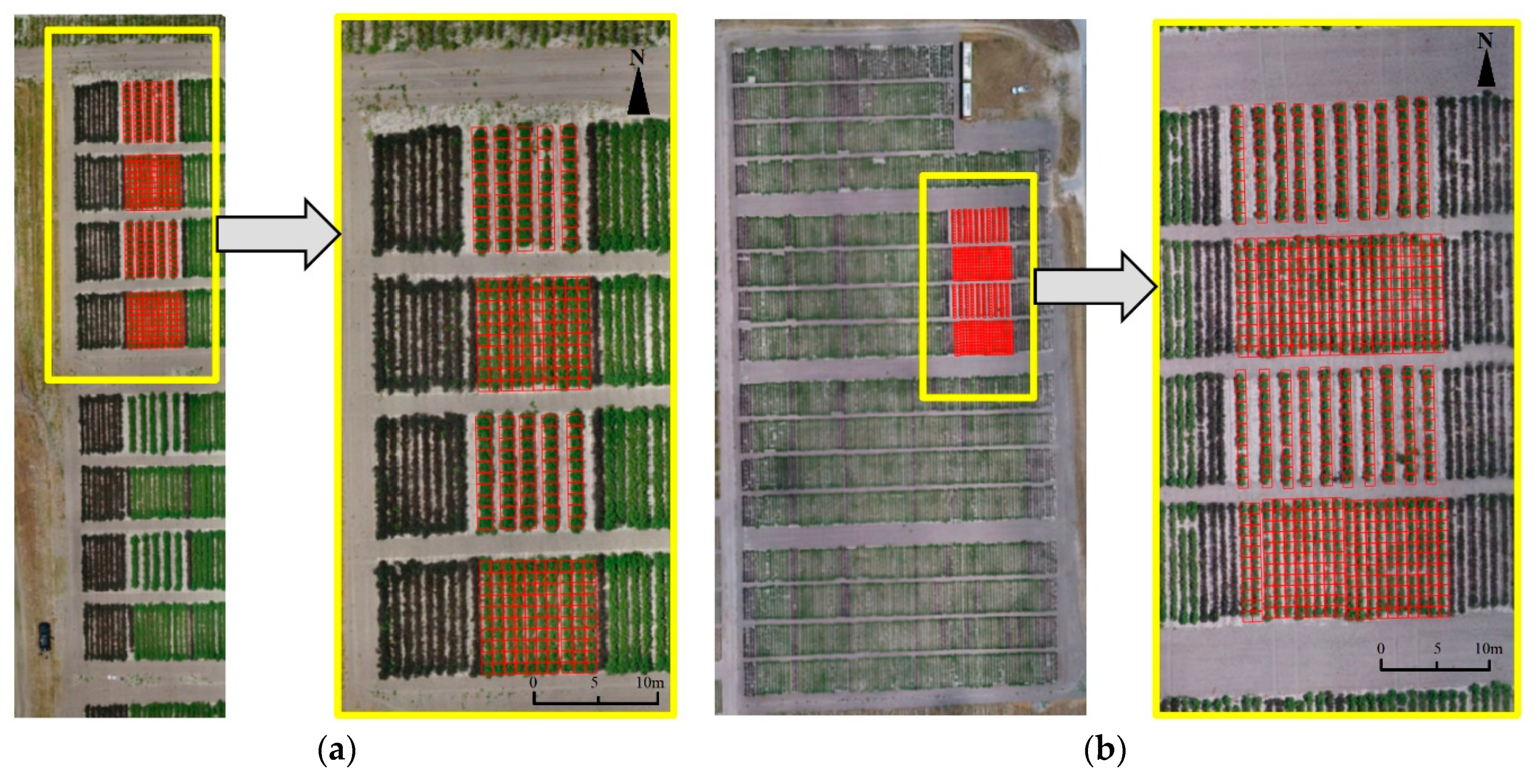
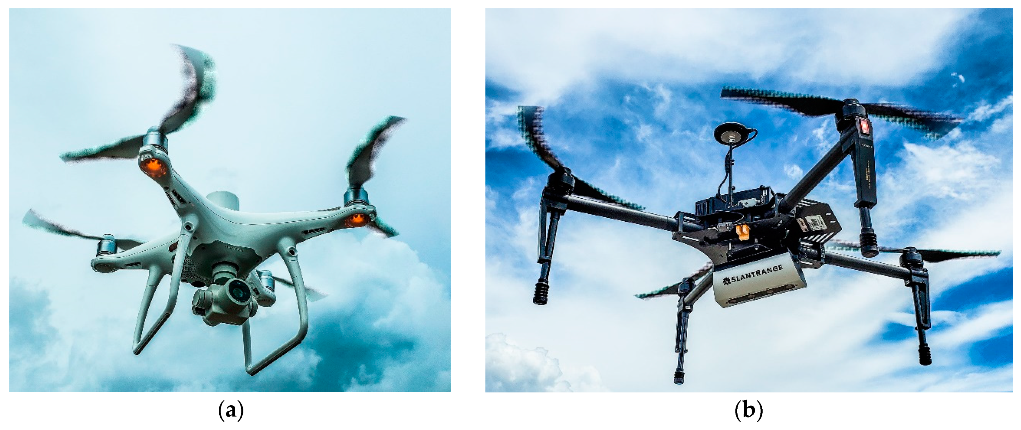
2.1. Study Area and Sensors

A field experiment was established at the Texas A&M AgriLife Research and Extension Center in Corpus Christi, TX (Latitude 27°46’59” N and longitude 97°34’13” W). The trial consisted of 5 cotton genotypes from the Texas A&M AgriLife Cotton Breeding Program (presented in Figure 1). Genotypes were planted 22 March 2017 in skip and solid row patterns (i.e., one- or two-row plots, respectively), and each was replicated four times. For canopy cover estimation, another field experiment was established at the same location in 2018. The trial consisted of 10 cotton genotypes from the Texas A&M AgriLife Cotton Breeding Program. Genotypes were planted in the first week of April in skip and solid row patterns. To maintain the integrity of the experiment, only part of the field which is highlighted by yellow boxes in Figure 1, was considered for both 2017 and 2018, as the selected area was the only area which had an alternate pattern of skip and non-skip rows and a common variety. The selected area was divided into 1 x 1 m size grids. The number of grids in 2017 and 2018 experiments was 300 and 600, respectively.
RGB and MS sensors were used for this study, as presented in Figure 2. A DJI Phantom 4 Pro (SZ DJI Technology Co., Ltd., Shenzhen, China) was used for RGB data collection. It comprised a 3-axis gimbal-stabilized RGB sensor with a resolution of 20 mega pixels. MS data were collected using the DJI Matrice 100 platform (SZ DJI Technology Co., Ltd., Shenzhen, China) with a SlantRange 3p sensor (Slantrange Inc, San Diego, CA) equipped with integrated solar spectrometer for frame-to-frame, radiometrically accurate reflectance measurements. The sensor has a spatial resolution of 4.8 cm/pixel at 120 m above ground level. It collects data using four spectral bands, namely green, red, red-edge, and near infrared bands, for which the peak wavelengths are presented in Table 1.

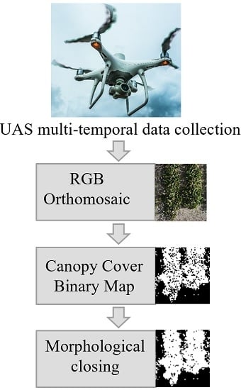
2.2. Data Collection and Preprocessing

Data collection and preprocessing was followed from the method of Ashapure et al. (2019) [31]. UAS data (both MS and RGB) were collected over the experimental field on a weekly basis. Table 2 presents the flight specifications for both RGB and MS data collection. A total of eleven and ten flights were conducted in 2017 and 2018, respectively, using RGB and MS sensors. The overlap for MS sensor data collection was 70%, and it was 80%–85% for RGB sensor data collection. In 2017, the altitude was about 20 m for the RGB sensor and 25 m for the MS sensor. In 2018, the flight altitude for RGB and MS sensors was 35 and 47 m, respectively. Provided the experimental field was in a coastal area, wind speed and rain were the potential factors to be considered before every flight. Most flights were conducted between 10:00AM and 2:00PM, except under unfavorable weather conditions, such as a wind speed greater than 15 mph or raining. Moreover, the temperature variation throughout the growing season varied between 79 and 96 °F.
Generally, UAS are equipped with a consumer grade global positioning system (GPS) that do not have satisfactory location accuracy for aerial mapping applications. To overcome this problem, semi-permanent ground control points (GCPs) with a high reflectance were installed over the study area. The GCPs were surveyed using a dual frequency, post processed kinematic (PPK) GPS system, 20 Hz V-Map Air model (Micro Aerial Project L.L.C., Gainesville, FL). Images obtained from the UAS platform with significant overlaps along with the 3D coordinates of the GCPs were imported to Agisoft Photoscan Pro (Agisoft LLC, St. Petersburg, Russia), which uses structure from motion (SfM) photogrammetry algorithms to derive high dens 3D point clouds, fine spatial resolution 2D orthomosaics, and digital surface models (DSM). The SfM refers to the process of finding the three-dimensional structure of an object by analyzing local motion signals over time [43].

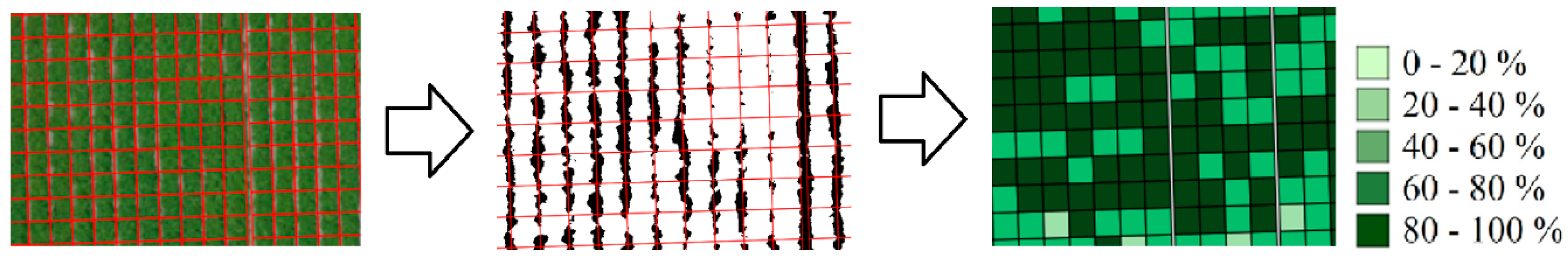
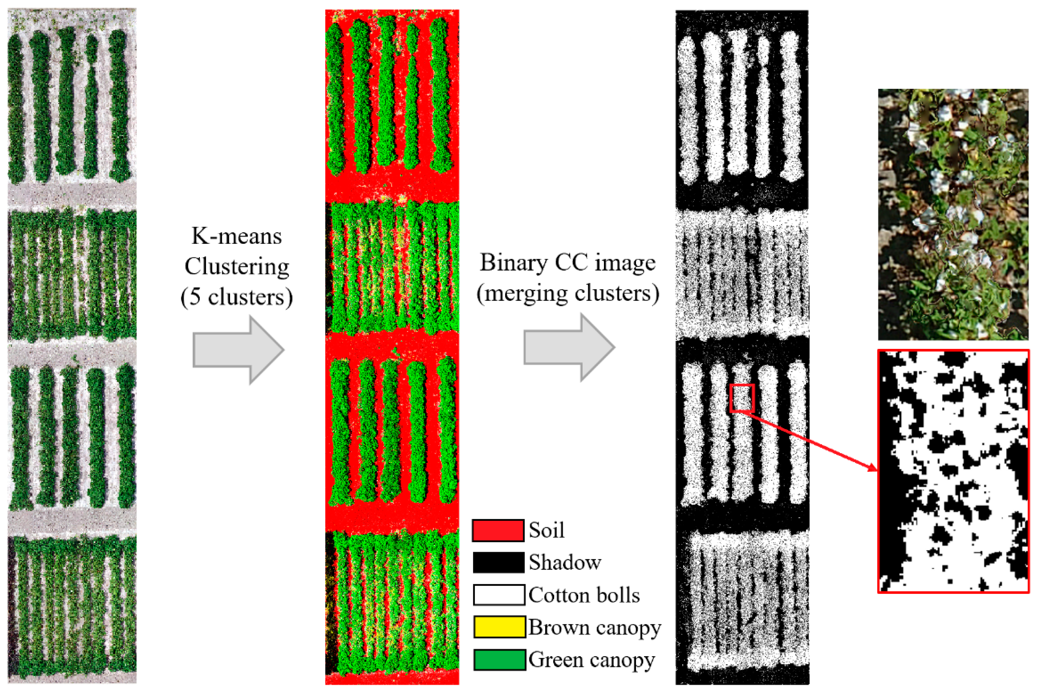
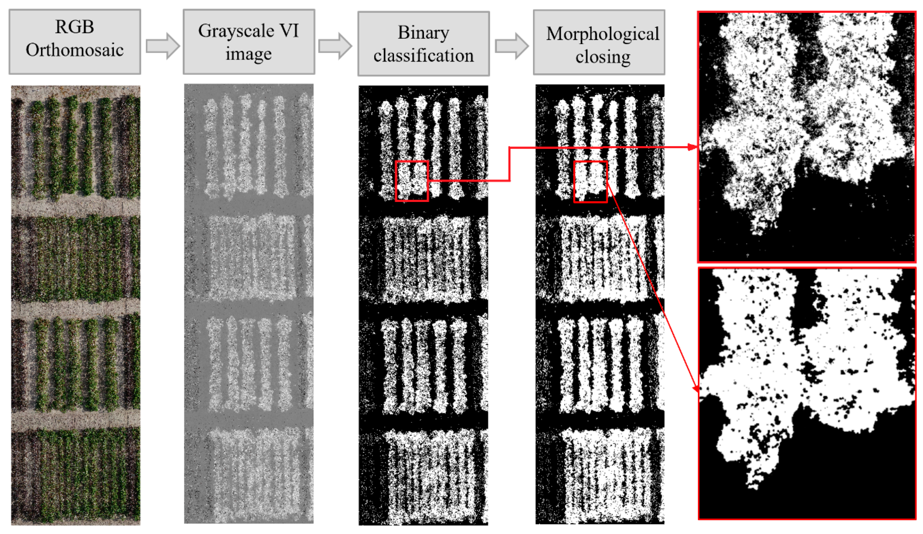
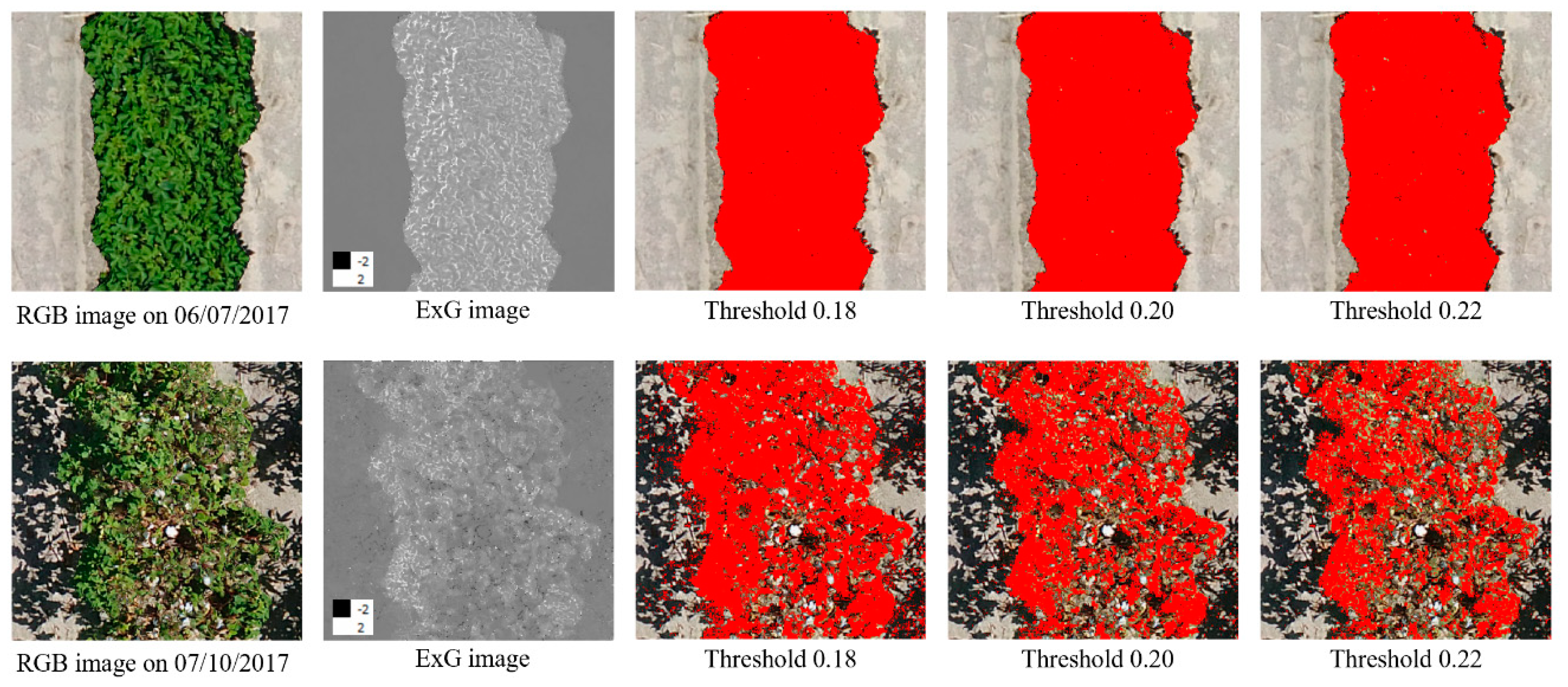
2.3. Canopy Cover Computation
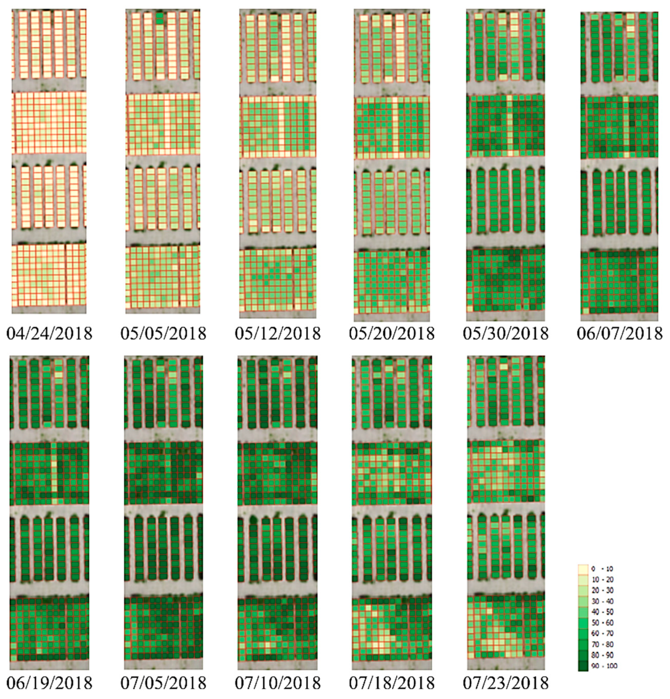
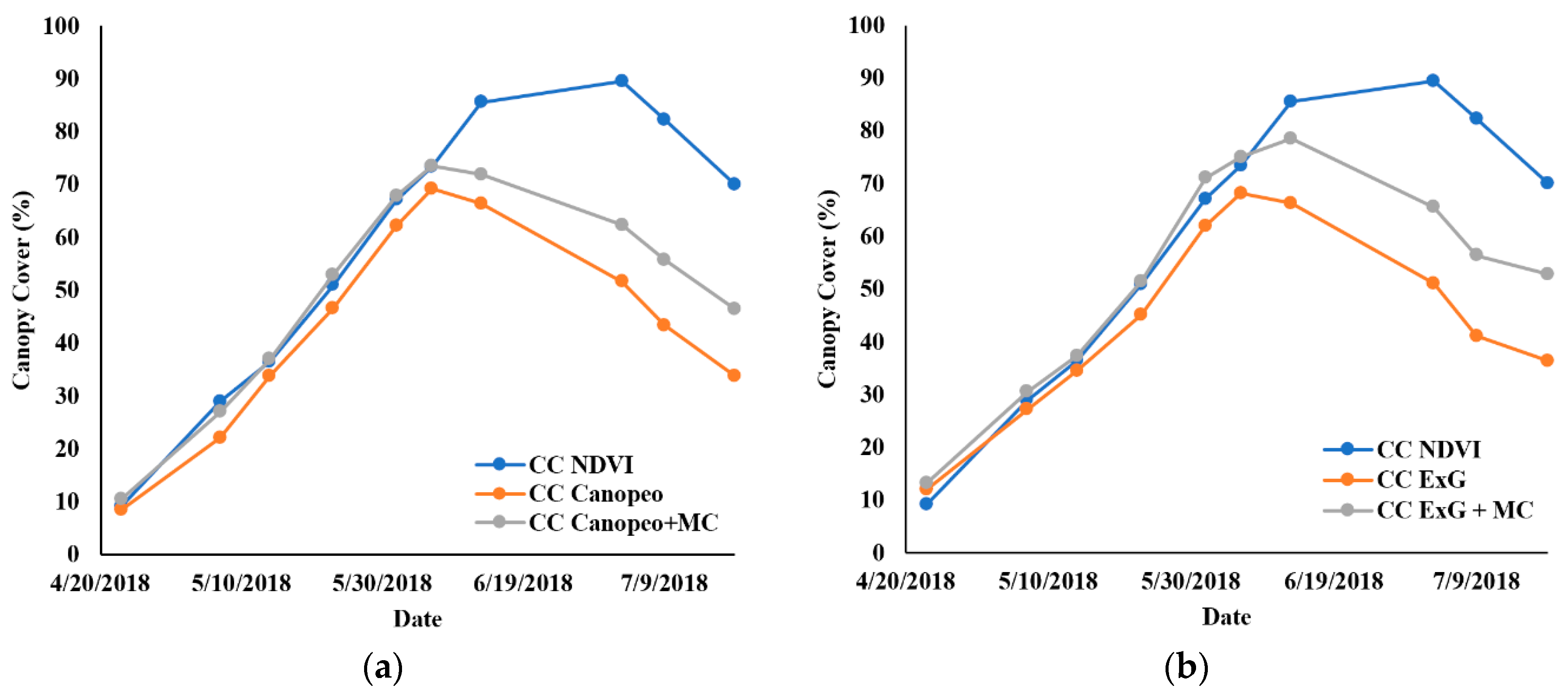
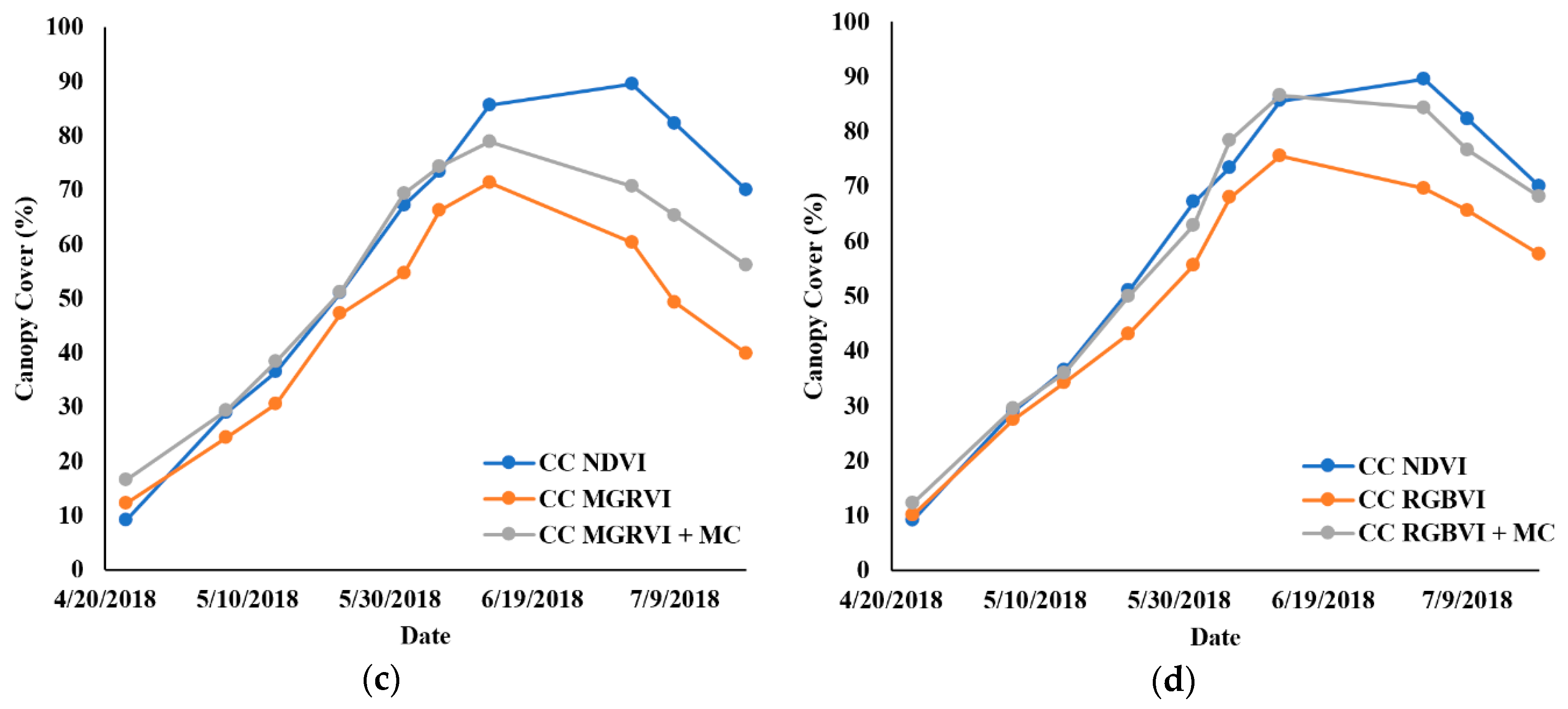
The percentage CC was computed as the ratio of canopy area to the total area of the grid computed using Equation (1), where GSD is ground sampling distance. An RGB orthomosaic image was converted into a binary image, where zero represents non-canopy pixels and one represents canopy pixels. As the whole field was divided into a square meter grid by using Equation (1), a grid-wise percentage CC was computed (As shown in Figure 3).
CC   = ( ( G C D 2 )     i f   C a n o p y   P i x e l ( G C D 2 )     ) × 100 ,
As mentioned earlier, MS sensor-based CC estimation is considered, in the literature, as the most reliable estimation technique that uses a normalized difference vegetation index (NDVI) to separate the canopy from the non-canopy areas (computed using Equation (2) [44]). SlantView, the software developed for the SlantRange 3p MS sensor, was used for the radiometric calibration in order to accurately compare the crop conditions across datasets collected in varying lighting conditions throughout the day and growing season. A detailed visual inspection was performed to find a threshold NDVI value to separate the canopy area from the non-canopy area in the image throughout the growing season regardless of the growth stage.
NDVI   = ( N I R R e d N I R + R e d   ) ,
To investigate the accurate CC estimation using the RGB-based sensor, which is equivalent to CC estimation using NDVI, a pixel-wise classification method was implemented; this is presented in Figure 4. As found in the literature, pixel classification methods are considered highly accurate for separating the canopy and non-canopy classes, and they are mainly used to calibrate RGB-based methods [35,38,45]. A pixel classification method based on K-means clustering was used to compare the RGB-based methods that use vegetation indices to separate canopy areas from non-canopy areas. Initially, K-means clustering with five classes was applied to the RGB orthomosaics, considering five potential classes representing soil, shadow, cotton bolls, green canopy and brown canopy, as presented in Figure 4. After assigning the class labels to the clustered map, it was validated using ground-truth samples collected over RGB orthomosaics using visual inspection, and the overall classification accuracy was found to be at least 97%. Later, soil, shadow and cotton bolls were merged and assigned as non-canopy, and green and brown canopy were merged and identified as canopy classes. However, as pixel-wise classification-based CC estimation is computationally extensive, its implementation was solely done with an intention to investigate the maximum achievable performance using the RGB-based sensors and to compare it with MS sensor-based CC estimation.
In this study, four different RGB-based methods were used, namely Canopeo, the excessive greenness index (ExG), the modified green red vegetation index (MGRVI) and the red green blue vegetation index (RGBVI), to generate the binary images to separate canopy areas from non-canopy areas (Table 3).
The overall procedure to compute the CC binary map using RGB vegetation indices is presented in Figure 5. The Canopeo algorithm resulted in a binary map that separated canopy areas from non-canopy areas; however, applying vegetation indices over the RGB mosaics resulted in a grayscale image. Similar to the NDVI, an empirical evaluation was performed over all the grey scale vegetation index maps to decide a threshold value for the ExG, the MGRVI and the RGBVI that could separate canopy areas from non-canopy areas. A detailed visual inspection was performed to determine a threshold value to separate canopy areas from non-canopy areas in the image throughout the growing season, regardless of the growth stage. Considering the homogeneity of the crop, only a subset of the image was used to determine the threshold, and the threshold chosen for each VI is presented in Table 4. The demonstration of visual inspection is presented in Figure 6, where a subset of an early stage and a mature stage RGB image of the same area is considered. Originally for all the RGB images in the growing season, a range of threshold values with a step size of 0.01 was applied to a subset area in the images to generate binary map using the grayscale VI map of the subset area. However, for the demonstration, only one VI (ExG) image was considered, and this was generated using one early stage (image taken on 7 June 2017) and one mature stage (image taken on 10 July 2017) RGB image with a range of threshold values and a step size of 0.02. It can be observed from Figure 6 that variation in threshold values did not affect the binarization of the early stage image, as most of the canopy was green. However with the higher threshold (0.22), the binary image had some canopy pixels not classified as canopy due to their darker color. The effect of variation in threshold was more significant in the mature stage image. A lower threshold value of 0.18 resulted in a lot of non-canopy pixels classified as canopy, especially the shadow pixels. A slightly higher threshold value of 0.22 resulted in more conservative classification that omitted a substantial number of canopy pixels. Visual inspection suggested that the threshold value of 0.2 resulted in a most appropriate classification for the ExG. Similarly, other VIs were also examined under visual inspection to select a single threshold value for all the images in the growing season.
RGB-based vegetation indices accurately identified healthy green canopy; however, later in the season as the canopy started to change the color, their ability to identify canopy deteriorated. To further improve the binary map (indicating canopy and non-canopy areas), a morphological closing operation was performed. The morphological closing operation is a combination of dilation and erosion, and it helps to remove small holes while keeping the separation boundary intact [48]. For this experiment, a 3 × 3 kernel window over one iteration was used to perform closing operation.

3. Results

The CC grid maps at each flight for both 2017 and 2018 are presented in Figure 7 and Figure 8, respectively. The visual inspection of the grid maps revealed that the percentage canopy cover increased in the growing season and reached its plateau right after the middle of the season (19 June for the 2017 experiment and 13 June for the 2018 experiment). Later in the season, it was observed that the percentage CC started to slightly decrease with the canopy senescence. For the 2017 experiment, a rapid decay in CC was observed between 18 July and 23 July due to a common practice in the cotton fields known as defoliation, which prepares the crop for harvesting. A similar effect was observed in the 2018 experiment between 9 July and 19 July.
Following the methodology presented in Figure 4 using RGB images, K-means clustering-based classification maps were generated considering five clusters which were later labeled to represent soil, cotton boll, shadow, green canopy, and brown canopy. Later, binary maps were generated by merging soil, cotton boll and shadow classes to indicate non-canopy, while brown canopy and green canopy classes were merged to indicate canopy pixels. The comparison of the average CC per grid using the NDVI and K-means (also referred as RGB reference) is presented in Figure 9 and Figure 10 for the 2017 and 2018 experiments, respectively. From both the 2017 and 2018 experiments, it was observed that the NDVI-based and RGB reference-based average CC per grid followed the same trend throughout the growing season, and there was a one-to-one correspondence between the two when plotted as a straight line at an intercept of one with very high R2 values (0.98 for 2017 and 0.97 for 2018). The results indicated that it is possible to achieve the same level of performance using the RGB-based sensor as that of the MS sensors using NDVI. However, the purpose of the RGB reference CC estimation was only to provide a comparison reference for the MS sensor-based CC estimation.
Using RGB images, four thresholding-based CC estimation methods were implemented, namely Canopeo, the ExG, the MGRVI and the RGBVI. Along with the NDVI-based average CC estimation per grid, the average CC estimation per grid in the growing season for each RGB-based CC estimation method before and after applying morphological closing (MC) is presented in Figure 11 and Figure 12 for the 2017 and 2018 experiments, respectively. It can be observed from Figure 11 that, early in the growing season, the average CC estimated by all the methods was in agreement with very less variation and followed the same increasing trend as the NDVI-based estimation. However, the Canopeo and ExG methods reached their peak early in the season (7th June), as compared to other methods. The main reason for this was that they were accurately identifying healthy green canopy, but later, as the canopy started to change color from green to yellow and eventually to brown, they were not as efficient as other methods to identify the matured canopy. Moreover, after they reached their peak, they rapidly started to decrease later in the season, commensurate with the rate of change of color in the canopy in the later season. As can be observed from Table 5, the average root mean square error (RMSE) of the percentage CC turned out to be highest amongst all (17.87 for Canopeo and 16.97 for the ExG). The MGRVI showed a slightly better performance over Canopeo and the ExG, and it was able to identify mature canopy. However, in comparison to the NDVI, it also reached its peak relatively early. The RGBVI turned out to be the most efficient method to estimate CC, as, especially later in the season, it outperformed the other RGB-based methods. However, the RGBVI still could not match the NDVI-based CC estimation. It was noticed that morphological closing significantly improved the CC estimation, and the average RMSE with the NDVI-based CC estimation was substantially reduced (Table 5).
A similar trend was observed in the performance of thresholding-based CC estimation methods in the 2018 experiment (Figure 12). Canopeo and the ExG method had the higher RMSE, as compared to other methods (Table 5). However, CC estimation values of 2018 experiment were slightly higher compared to CC estimation values of 2017 experiment. The RGBVI turned out to be the most efficient CC estimation method amongst all. The application of the morphological closing operation significantly reduced the RMSE. It was observed that morphological closing operation resulted in slightly better performance in the 2018 experiment as compared to the 2017 experiment. It was noticed that in the 2018 experiments, the spatial resolution of the RGB images was slightly lower than the 2017 experiments. However, the difference in the spatial resolution was not much (difference of ~0.2cm), and a slight decrease of the GSD might contribute to the better classification and later filtering performance because a very high resolution leads to more details being observed, which could be undesirable when the information class under consideration is more general. Furthermore, a little difference in the CC growth pattern in two years was observed, which was a function of weather conditions (such as daily temperature and precipitation) and the type of genotype planted.

4. Discussion

Recent years have witnessed an upsurge in UAS and sensor technology, an upsurge which has made it possible to collect high temporal and spatial resolution data over crops throughout the growing season. The main objective of this study was to provide a comparison framework between MS sensor-based CC estimation and RGB-based CC estimation, as very scarce attention has been paid to explore different VIs generated using UAS-based sensors to compute canopy cover in the literature. As mentioned in the literature, MS sensor-based CC estimation is more accurate and stable because it accounts for the live canopy based on the chlorophyll content present in the canopy, and this content is highly reflected in the near-infrared (NIR) band; hence, the canopy varieties which are not green in color can be correctly accounted for. Moreover, changes in the color as the season progresses can also be identified accurately. However, the accuracy of the NDVI is a function of the type and quality of the multispectral sensor used to collect the image. In this study, temporal NDVI maps were comparable, despite changes in lighting conditions over different flights throughout the season, as they were generated from multispectral data collected using the SlantRange 3p sensor that performed radiometric calibration. The RGB-based CC estimation performed inadequately if the plant color deviated from green, which was confirmed by the experiments performed in both 2017 and 2018.
Except for the Canopeo method, all the other RGB VIs considered in this study required a threshold to be applied in order to separate canopy areas from non-canopy areas. In previous studies, the Otsu method has mostly been used for automatic thresholding [41]. The Otsu method resulted in an accurate thresholding early in the season, as the image had a mostly bimodal histogram and the variances of the spectral clusters were small compared to the mean difference. However, later in the season, thresholding by the Otsu method was questionable, because, as the season progressed, the variance in the spectral signature of the canopy increased, and, closer to senescence, the image no longer possessed a bimodal histogram due to the emergence of new spectral classes such as open cotton bolls. Consequently, in this study, the VIs were examined under visual inspection to select a single threshold value for all the images in the growing season. It was observed that the selected single threshold value successfully classified canopy pixels. Though they were less affected due to senescence as compared to the RGB-based VIs, the overall NDVI values still decreased in the late season; however, the selected single threshold value successfully classified canopy pixels with reasonable accuracy based on visual interpretation. Since this study was limited to the cotton crop, the threshold value might differ for other crops, and there might be a different trend observed in response to the senescence in the growing season. In future, an efficient thresholding method that can classify canopy regardless of growth stage would help automate the process.
As previous studies have affirmed that RGB-based CC estimation efficiently works early in the season [40,41], it was also observed in this study that early in the season, both the MS- and RGB-based CC estimations were in agreement and followed a similar increasing trend. Moreover, in previous studies, MS sensor-based CC estimation has been found to be more accurate in the later season as compared to RGB-based CC estimation [41]. In this study, it was observed that as the season progressed, MS sensor-based CC estimation kept on increasing, but RGB-based CC estimation peaked early and started to drop relatively rapidly for both the 2017 and 2018 experiments. Nevertheless, the RGBVI outperformed other RBG-based CC estimation methods, though still not close enough to match the estimation by MS sensor-based CC estimation. That led to the question “is it possible to achieve the same level of accuracy by using RGB-based CC estimation as that of the NDVI-based CC estimation?” With the aforementioned objective, a K-means clustering-based CC estimation method was implemented, and this was tested by using ground truth samples for the canopy and non-canopy classes. It was observed that K-means clustering-based approach matched the accuracy level of the MS sensor-based CC estimation. However, there was a requirement to investigate any scope for an improvement to the RGB-based CC estimation approach, as the K-means clustering-based approach, or any classification-based approach is accurate but computationally extensive, especially in its parameter tuning and demand for ground truth sample collection, which is labor-intensive and time consuming. The objective of this study was to improve the RGB-based CC estimation approach. It was noticed that, later in the season, RGB-based indices were not able to capture the canopy pixels that were not green, which resulted in CC maps with a lot of small holes. The morphological closing operation proved to be a solution to this problem and helped to fill very small holes and keep the boundary of the canopy intact. In both the 2017 and 2018 experiments, it was noticed that applying the morphological closing operation significantly improved the performance of the RGB-based CC estimation. The RGBVI with morphological closing applied was found to have a CC estimation very close to the NDVI-based CC estimation. With the proposed approach, a more affordable alternate to the MS sensor can be provided to estimate CC.

5. Conclusions

A comparative study was performed to evaluate CC estimation using an RGB sensor. With a multi-year CC analysis, MS sensor-based CC estimation was used as a reference, as it is considered a stable and accurate form of estimation. The correlation of RGB reference-based CC estimation with MS sensor-based CC estimation ensured the feasibility of using an RGB sensor to match the MS sensor-based CC estimation. An analysis of RGB-based methods suggested that the RGBVI was more tolerant to changes in the color of the canopy when the canopy started to senescence. Moreover, when applied with the morphological closing operation, the RGBVI-based CC estimation was found to be as accurate as MS sensor-based CC estimation, with an average RMSE of less than three percent. CC is a good predictor variable for plant growth parameters. As multispectral sensors are more sensitive and expensive, the proposed RGB-based CC estimation could provide an affordable alternate to agriculture scientists and breeders. In the future, this methodology will be investigated on other crops, as there might be a different trend observed in response to senescence in the growing season.

Author Contributions

conceptualization, A.A. and J.J.; data curation, A.A., A.C. and S.O.; formal analysis, A.A.; investigation, M.M.; methodology, A.A. and J.J.; project administration, J.J., M.M. and J.L.; resources, J.L.; software, A.A.; supervision, J.J.; validation, A.A.; visualization, A.A.; writing—original draft, A.A.; writing—review & editing, J.J., A.C., S.O. and J.L.

Funding

This research received no external funding.

Acknowledgments

This research was supported by Texas A&M AgriLife Research, Corpus Christi.

Conflicts of Interest

The authors declare no conflict of interest.

References

  1. Adhikari, P.; Gowda, P.; Marek, G.; Brauer, D.; Kisekka, I.; Northup, B.; Rocateli, A. Calibration and validation of csm-cropgro-cotton model using lysimeter data in the texas high plains. J. Contemp. Water Res. Educ. 2017, 162, 61–78. [Google Scholar] [CrossRef]
  2. Phillips, R.L. Mobilizing science to break yield barriers. Crop Sci. 2010, 50, 99–108. [Google Scholar] [CrossRef]
  3. Xu, R.; Li, C.; Paterson, A.H. Multispectral imaging and unmanned aerial systems for cotton plant phenotyping. PLoS ONE 2019, 14, e0205083. [Google Scholar] [CrossRef] [PubMed]
  4. Pierpaoli, E.; Carli, G.; Pignatti, E.; Canavari, M. Drivers of precision agriculture technologies adoption: A literature review. Procedia Technol. 2013, 8, 61–69. [Google Scholar] [CrossRef]
  5. Tokekar, P.; Vander Hook, J.; Mulla, D.; Isler, V. Sensor planning for a symbiotic uav and ugv system for precision agriculture. IEEE Trans. Robot. 2016, 32, 1498–1511. [Google Scholar] [CrossRef]
  6. Singh, K.K.; Frazier, A.E. A meta-analysis and review of unmanned aircraft system (uas) imagery for terrestrial applications. Int. J. Remote Sens. 2018, 39, 5078–5098. [Google Scholar] [CrossRef]
  7. Roth, L.; Streit, B. Predicting cover crop biomass by lightweight uas-based rgb and nir photography: An applied photogrammetric approach. Precis. Agric. 2018, 19, 93–114. [Google Scholar] [CrossRef]
  8. Gevaert, C.M.; Suomalainen, J.; Tang, J.; Kooistra, L. Generation of spectral–temporal response surfaces by combining multispectral satellite and hyperspectral uav imagery for precision agriculture applications. IEEE J. Sel. Top. Appl. Earth Obs. Remote Sens. 2015, 8, 3140–3146. [Google Scholar] [CrossRef]
  9. Trout, T.J.; Johnson, L.F.; Gartung, J. Remote sensing of canopy cover in horticultural crops. HortScience 2008, 43, 333–337. [Google Scholar] [CrossRef]
  10. Nielsen, D.C.; Miceli-Garcia, J.J.; Lyon, D.J. Canopy cover and leaf area index relationships for wheat, triticale, and corn. Agron. J. 2012, 104, 1569–1573. [Google Scholar] [CrossRef]
  11. Chopping, M. Canapi: Canopy analysis with panchromatic imagery. Remote Sens. Lett. 2011, 2, 21–29. [Google Scholar] [CrossRef]
  12. Halperin, J.; LeMay, V.; Chidumayo, E.; Verchot, L.; Marshall, P. Model-based estimation of above-ground biomass in the miombo ecoregion of zambia. For. Ecosyst. 2016, 3, 14. [Google Scholar] [CrossRef]
  13. Hansen, M.C.; DeFries, R.S.; Townshend, J.R.; Carroll, M.; DiMiceli, C.; Sohlberg, R.A. Global percent tree cover at a spatial resolution of 500 meters: First results of the modis vegetation continuous fields algorithm. Earth Interact. 2003, 7, 1–15. [Google Scholar] [CrossRef]
  14. Korhonen, L.; Hovi, A.; Rönnholm, P.; Rautiainen, M. The accuracy of large-area forest canopy cover estimation using landsat in boreal region. Int. J. Appl. Earth Obs. Geoinf. 2016, 53, 118–127. [Google Scholar]
  15. Chemura, A.; Mutanga, O.; Odindi, J. Empirical modeling of leaf chlorophyll content in coffee (coffea arabica) plantations with sentinel-2 msi data: Effects of spectral settings, spatial resolution, and crop canopy cover. IEEE J. Sel. Top. Appl. Earth Obs. Remote Sens. 2017, 10, 5541–5550. [Google Scholar] [CrossRef]
  16. Melin, M.; Korhonen, L.; Kukkonen, M.; Packalen, P. Assessing the performance of aerial image point cloud and spectral metrics in predicting boreal forest canopy cover. ISPRS J. Photogramm. Remote Sens. 2017, 129, 77–85. [Google Scholar] [CrossRef]
  17. Korhonen, L.; Ali-Sisto, D.; Tokola, T. Tropical forest canopy cover estimation using satellite imagery and airborne lidar reference data. Silva Fenn. 2015, 49, 1–18. [Google Scholar] [CrossRef]
  18. Li, W.; Niu, Z.; Huang, N.; Wang, C.; Gao, S.; Wu, C. Airborne lidar technique for estimating biomass components of maize: A case study in zhangye city, northwest china. Ecol. Indic. 2015, 57, 486–496. [Google Scholar] [CrossRef]
  19. Tattaris, M.; Reynolds, M.P.; Chapman, S.C. A direct comparison of remote sensing approaches for high-throughput phenotyping in plant breeding. Front. Plant Sci. 2016, 7, 1131. [Google Scholar] [CrossRef]
  20. Chen, A.; Orlov-Levin, V.; Elharar, O.; Meron, M. Comparing satellite and high-resolution visible and thermal aerial imaging of field crops for precision irrigation management and plant biomass forecast. In Precision Agriculture’19; Wageningen Academic Publishers: Wageningen, The Netherlands, 2019; pp. 37–44. [Google Scholar]
  21. Korhonen, L.; Korpela, I.; Heiskanen, J.; Maltamo, M. Airborne discrete-return lidar data in the estimation of vertical canopy cover, angular canopy closure and leaf area index. Remote Sens. Environ. 2011, 115, 1065–1080. [Google Scholar] [CrossRef]
  22. Anderson, K.E.; Glenn, N.F.; Spaete, L.P.; Shinneman, D.J.; Pilliod, D.S.; Arkle, R.S.; McIlroy, S.K.; Derryberry, D.R. Estimating vegetation biomass and cover across large plots in shrub and grass dominated drylands using terrestrial lidar and machine learning. Ecol. Indic. 2018, 84, 793–802. [Google Scholar] [CrossRef]
  23. Ma, Q.; Su, Y.; Guo, Q. Comparison of canopy cover estimations from airborne lidar, aerial imagery, and satellite imagery. IEEE J. Sel. Top. Appl. Earth Obs. Remote Sens. 2017, 10, 4225–4236. [Google Scholar] [CrossRef]
  24. Holman, F.; Riche, A.; Michalski, A.; Castle, M.; Wooster, M.; Hawkesford, M. High throughput field phenotyping of wheat plant height and growth rate in field plot trials using uav based remote sensing. Remote Sens. 2016, 8, 1031. [Google Scholar] [CrossRef]
  25. Chianucci, F.; Disperati, L.; Guzzi, D.; Bianchini, D.; Nardino, V.; Lastri, C.; Rindinella, A.; Corona, P. Estimation of canopy attributes in beech forests using true colour digital images from a small fixed-wing uav. Int. J. Appl. Earth Obs. Geoinf. 2016, 47, 60–68. [Google Scholar] [CrossRef]
  26. Fernandez-Gallego, J.A.; Kefauver, S.C.; Kerfal, S.; Araus, J.L. Remote Sensing for Agriculture, Ecosystems, and Hydrology XX. In Comparative Canopy Cover Estimation Using RGB Images from UAV and Ground; International Society for Optics and Photonics: Berlin, Germany, 2018; p. 107830J. [Google Scholar]
  27. Ashapure, A.; Oh, S.; Marconi, T.G.; Chang, A.; Jung, J.; Landivar, J.; Enciso, J. Autonomous Air and Ground Sensing Systems for Agricultural Optimization and Phenotyping IV. In Unmanned Aerial System Based Tomato Yield Estimation Using Machine Learning; International Society for Optics and Photonics: Baltimore, MD, USA, 2019. [Google Scholar]
  28. Chu, T.; Chen, R.; Landivar, J.A.; Maeda, M.M.; Yang, C.; Starek, M.J. Cotton growth modeling and assessment using unmanned aircraft system visual-band imagery. J. Appl. Remote Sens. 2016, 10, 036018. [Google Scholar] [CrossRef]
  29. Ballesteros, R.; Ortega, J.; Hernández, D.; Moreno, M. Applications of georeferenced high-resolution images obtained with unmanned aerial vehicles. Part II: Application to maize and onion crops of a semi-arid region in spain. Precis. Agric. 2014, 15, 593–614. [Google Scholar] [CrossRef]
  30. Ballesteros, R.; Ortega, J.F.; Hernandez, D.; Moreno, M.A. Onion biomass monitoring using uav-based rgb imaging. Precis. Agric. 2018, 19, 840–857. [Google Scholar] [CrossRef]
  31. Ashapure, A.; Jung, J.; Yeom, J.; Chang, A.; Maeda, M.; Maeda, A.; Landivar, J. A novel framework to detect conventional tillage and no-tillage cropping system effect on cotton growth and development using multi-temporal uas data. ISPRS J. Photogramm. Remote Sens. 2019, 152, 49–64. [Google Scholar] [CrossRef]
  32. Makanza, R.; Zaman-Allah, M.; Cairns, J.; Magorokosho, C.; Tarekegne, A.; Olsen, M.; Prasanna, B. High-throughput phenotyping of canopy cover and senescence in maize field trials using aerial digital canopy imaging. Remote Sens. 2018, 10, 330. [Google Scholar] [CrossRef]
  33. Clevers, J.; Kooistra, L.; Van Den Brande, M. Using sentinel-2 data for retrieving lai and leaf and canopy chlorophyll content of a potato crop. Remote Sens. 2017, 9, 405. [Google Scholar] [CrossRef]
  34. Pauly, K. Applying conventional vegetation vigor indices to uas-derived orthomosaics: Issues and considerations. In Proceedings of the International Conference of Precision Agriculture (ICPA), Sacramento, CA, USA, 20–23 July 2014. [Google Scholar]
  35. Booth, D.T.; Cox, S.E.; Berryman, R.D. Point sampling digital imagery with ‘samplepoint’. Environ. Monit. Assess. 2006, 123, 97–108. [Google Scholar] [CrossRef] [PubMed]
  36. Richardson, M.; Karcher, D.; Purcell, L. Quantifying turfgrass cover using digital image analysis. Crop Sci. 2001, 41, 1884–1888. [Google Scholar] [CrossRef]
  37. Lee, K.J.; Lee, B.W. Estimating canopy cover from color digital camera image of rice field. J. Crop Sci. Biotechnol. 2011, 14, 151–155. [Google Scholar] [CrossRef]
  38. Patrignani, A.; Ochsner, T.E. Canopeo: A powerful new tool for measuring fractional green canopy cover. Agron. J. 2015, 107, 2312–2320. [Google Scholar] [CrossRef] [Green Version]
  39. Torres-Sánchez, J.; Peña, J.M.; de Castro, A.I.; López-Granados, F. Multi-temporal mapping of the vegetation fraction in early-season wheat fields using images from uav. Comput. Electron. Agric. 2014, 103, 104–113. [Google Scholar] [CrossRef]
  40. Fang, S.; Tang, W.; Peng, Y.; Gong, Y.; Dai, C.; Chai, R.; Liu, K. Remote estimation of vegetation fraction and flower fraction in oilseed rape with unmanned aerial vehicle data. Remote Sens. 2016, 8, 416. [Google Scholar] [CrossRef] [Green Version]
  41. Marcial-Pablo, M.D.J.; Gonzalez-Sanchez, A.; Jimenez-Jimenez, S.I.; Ontiveros-Capurata, R.E.; Ojeda-Bustamante, W. Estimation of vegetation fraction using rgb and multispectral images from uav. Int. J. Remote Sens. 2019, 40, 420–438. [Google Scholar] [CrossRef]
  42. Lima-Cueto, F.J.; Blanco-Sepúlveda, R.; Gómez-Moreno, M.L.; Galacho-Jiménez, F.B. Using vegetation indices and a uav imaging platform to quantify the density of vegetation ground cover in olive groves (Olea europaea L.) in southern spain. Remote Sens. 2019, 11, 2564. [Google Scholar] [CrossRef] [Green Version]
  43. Westoby, M.J.; Brasington, J.; Glasser, N.F.; Hambrey, M.J.; Reynolds, J.M. ‘Structure-from-motion’photogrammetry: A low-cost, effective tool for geoscience applications. Geomorphology 2012, 179, 300–314. [Google Scholar] [CrossRef] [Green Version]
  44. Rouse, J.W., Jr.; Haas, R.; Schell, J.; Deering, D. Monitoring Vegetation Systems in the Great Plains with ERTS; Texas A&M Univ.: College Station, TX, USA, 1974. [Google Scholar]
  45. Hulvey, K.B.; Thomas, K.; Thacker, E. A comparison of two herbaceous cover sampling methods to assess ecosystem services in high-shrub rangelands: Photography-based grid point intercept (gpi) versus quadrat sampling. Rangelands 2018, 40, 152–159. [Google Scholar] [CrossRef]
  46. Woebbecke, D.M.; Meyer, G.E.; Von Bargen, K.; Mortensen, D. Color indices for weed identification under various soil, residue, and lighting conditions. Trans. ASAE 1995, 38, 259–269. [Google Scholar] [CrossRef]
  47. Bendig, J.; Yu, K.; Aasen, H.; Bolten, A.; Bennertz, S.; Broscheit, J.; Gnyp, M.L.; Bareth, G. Combining uav-based plant height from crop surface models, visible, and near infrared vegetation indices for biomass monitoring in barley. Int. J. Appl. Earth Obs. Geoinf. 2015, 39, 79–87. [Google Scholar] [CrossRef]
  48. Dougherty, E.R. An Introduction to Morphological Image Processing; SPIE: Bellingham, WA, USA, 1992. [Google Scholar]
Figure 1. Experimental field setup consisted of cotton in skip and solid row patterns in: (a) 2017 and (b) 2018. The experimental field setup is presented with an RGB (red, green, and blue) orthomosaic of the study area on June 7, 2017, and June 6, 2018.
Remotesensing 11 02757 g001
Figure 2. RGB and multispectral sensors used for data collection. (a) The DJI Phantom 4 Pro for RGB and (b) the DJI Matrice 100 platform with the SlantRange 3p sensor for multispectral data collection.
Remotesensing 11 02757 g002
Figure 3. Canopy cover estimation from the orthomosaic images (Red square: individual crop grid, and each grid is 1 × 1 m): an RGB orthomosaic image collected using the unmanned aerial systems (UAS) platform, followed by the binary classification results of the orthomosaic image, where white represents the canopy class and black represents the non-canopy class; the last image represents the grid-wise estimated canopy cover (CC).
Remotesensing 11 02757 g003
Figure 4. K-means clustering-based pixel classification method workflow where the orthomosaic is classified into five classes, and, later, classes are merged into two clusters, namely canopy and non-canopy. The RGB orthomosaic presented was captured on 19th June 2017.
Remotesensing 11 02757 g004
Figure 5. Procedure to generate a binary map that indicates canopy and non-canopy areas. Applying the vegetation index over the RGB orthomosaic resulted in a grayscale image. By applying thresholding, a binary image was generated. Lastly, morphological closing was applied over binary image to improve binary classification. The presented RGB orthomosaic was captured on 10 July 2017, and the excessive greenness index (ExG) was the VI used for the demonstration of the methodology.
Remotesensing 11 02757 g005
Figure 6. Procedure to select appropriate threshold value to generate a binary map that indicates canopy and non-canopy areas. The first images are a subset of RGB images captured on 7 June 2017 and 10 July 2017. Second images are the result of applying the vegetation index (ExG) over RGB images. The next three images are the result of applying varying threshold values that were superimposed on the original RGB images (the canopy classified pixels are represented by the red color, and non-canopy pixels were set to transparent).
Remotesensing 11 02757 g006
Figure 7. CC grid maps generated at each flight in growing season using normalized difference vegetation index (NDVI) maps for the 2017 dataset.
Remotesensing 11 02757 g007
Figure 8. CC grid maps generated at each flight in growing season using NDVI maps for the 2018 dataset.
Remotesensing 11 02757 g008
Figure 9. For the 2017 experiment: (a) the average NDVI and RGB reference-based percentage CC for each flight in the growing season; (b) a comparison of the NDVI and RGB reference-based percentage CC techniques with R2.
Remotesensing 11 02757 g009
Figure 10. For the 2018 experiment: (a) the average NDVI and RGB reference-based percentage CC for each flight in the growing season; (b) a comparison of the NDVI and RGB reference-based percentage CC techniques with R2.
Remotesensing 11 02757 g010
Figure 11. For the 2017 experiment, the average CC estimation per grid using the NDVI-based CC estimation throughout the growing season, along with the average CC estimation using (a) Canopeo, (b) the ExG, (c) the modified green red vegetation index (MGRVI) and (d) the red green blue vegetation index (RGBVI), before and after applying the morphological closing (MC) operation.
Remotesensing 11 02757 g011
Figure 12. For the 2018 experiment, the average CC estimation per grid using the NDVI-based CC estimation throughout the growing season, along with the average CC estimation using (a) Canopeo, (b) the ExG, (c) the MGRVI and (d) the RGBVI, before and after applying the morphological closing (MC) operation.
Remotesensing 11 02757 g012aRemotesensing 11 02757 g012b
Table 1. Peak wavelength and FWHM (full width at half maximum) for SlantRange 3p sensor bands.
SlantRange 3p Sensor Band Peak Wavelength (nm) FWHM (nm)
Green56040
Red65535
Red-edge71020
Near infrared830110
Table 2. UAS data collection timeline and sensor-wise flight specification.
DateFlight Altitude (m)Overlap (%)Spatial Resolution (cm)
RGBMultispectralRGBMultispectralRGBMultispectral
24 April 2017203085750.510.93
5 May 2017202585700.500.85
12 May 2017202585700.510.81
20 May 2017202585700.520.82
30 May 2017202585700.510.85
7 June 2017202585700.510.83
19 June 2017202585700.520.81
5 July 2017202585700.510.81
10 July 2017202585700.500.83
18 July 2017202585700.510.82
23 July 2017202585700.510.82
23 April 2018354780700.731.61
7 May 2018354780700.691.65
14 May 2018354780700.711.61
23 May 2018354780700.711.64
1 June 2018374780700.731.62
6 June 2018354780700.721.61
13 June 2018354780700.711.63
3 July 2018354780700.711.61
9 July 2018354780700.721.63
19 July 2018354780700.701.62
Table 3. RGB image-based vegetation indices and their formula.
Vegetation Index Formula Reference
Canopeo c a n o p y = ( i 1 < θ 2 ) × ( i 2 < θ 1 ) × ( i 3 > θ 3 )
i 1 = r e d g r e e n , i 2 = b l u e g r e e n ,     i 3 = 2 × g r e e n b l u e r e d
  θ 1 = 0.95 ,     θ 2 = 0.95 ,   θ 3 = 20
[38]
ExG2 G n R n B n  
R n = R R + G + B , G n = G R + G + B , B n = B R + G + B
[46]
MGRVI G 2 R 2 G 2 + R 2 [47]
RGBVI G 2 R × B G 2 + R × B [47]
Table 4. Threshold chosen for vegetation indices (Vis) to separate canopy and non-canopy areas.
VIThreshold Range
NDVI0.60 to 1
ExG0.2−2 to 2
MGRVI0.15−1 to 1
RGBVI0.15−1 to 1
Table 5. Average RMSE of the thresholding-based CC estimation methods with respect to the NDVI-based CC estimation (%) throughout the growing season.
RGB-Based MethodAverage RMSE with Respect to NDVI-Based CC Estimation (%)
2017 Experiment2018 Experiment
Before MCAfter MCBefore MCAfter MC
Canopeo 17.8713.3415.569.73
ExG 16.9713.0015.518.67
MGRVI 13.1110.3514.346.95
RGBVI 7.442.948.852.82

