Experimental Validation of GNSS Interferometric Radio Occultation

Abstract

In this work, we present experimental results on the interferometric radio occultation (iRO) signal processing techniques, and compare the performance to the closed-loop and open-loop processing used in conventional radio occultation measurements. We also discuss the effects of antenna beam width to mitigate inter-satellite interferences, as well as how the local oscillator stability affects the obtained Doppler estimates. The required signal processing resources are less stringent for the iRO than for conventional RO techniques. In addition, the zenith iRO has a comparable performance to the well-established RO techniques.

1. Introduction

The first radio-occultation (RO) measurements to sense the atmosphere of planets were carried out in 1965, while the first GPS radio-occultation measurements to sense the Earth atmosphere were done in 1995 in the frame of the GPS/MET experiment. Since this first experimental validation, the concept has been highly successful, and it has been used in many satellites and missions, e.g., [1]. These types of measurements are important in operational meteorology, where its assimilation in numerical weather prediction (NWP) models significantly improves the performance of the predictions, e.g., [2,3,4]. Furthermore, long series of RO observations have allowed to observe the temperature trends of the stratosphere, e.g., [5]. The success of RO measurements has fostered the definition of new measurement concepts to improve and expand the range of applications, as for instance the measurement of the higher ionosphere, e.g., [6], or the measurement of heavy precipitation using polarimetric RO measurements [7].

Electromagnetic signals traveling through a medium experience a longer electrical path compared to signals that propagate in vacuum. When the density of the medium is a function of position (or altitude in case of the atmosphere) it will affect the electrical path in more or less degree depending through which part the electromagnetic radiation has traveled. By measuring with high precision the change of the electrical path it is possible to extract its density profile. In GPS RO, the fundamental measurement principle consists in obtaining precise phase delay measurements, which are directly linked to electrical path length and their change.

The inherent properties of the transmitted signals, which were designed to allow precise delay measurements, are used in GPS RO. The received signal is cross-correlated with a local replica (generated at the receiving satellite) of the expected signal. This implies that the receiver has to know the actual transmitted signal in order to be able to generate a local replica of it. In addition, it needs to know its current position and velocity, and the one of the transmitter to be able to generate this local replica with enough accuracy. The phase of the resulting complex cross-correlation value provides the phase estimate with respect to the applied open-loop model, and it is thus the observable that carries information with physical meaning of the medium through which the signal has traveled.

A new signal processing method was proposed in [8], presenting the interferometric RO (iRO) in the frame of the proposed GEROS-ISS mission, whose primary objective is the GNSS reflectometry (GNSS-R) to obtain ocean altimetry measurements. The instrumental architecture of GEROS-ISS is particularly conceived for high precision altimetry, using only open-loop delay and Doppler compensated cross-correlation between the received direct and reflected signals. Ref. [8] proposed a processing technique which reusing the hardware of the GEROS-ISS instrument enables phase delay measurements of GNSS signals. In this case the technique uses the periodic properties of the GNSS signals, and does not require to know the actual transmitted signal. The instrument requires also high gain antennas. In this paper, we present experimental work demonstrating the capabilities and limitations of this technique. Currently, ESA is developing PRETTY, an interferometric reflectometry GNSS mission with the antenna pointing to the limb of the Earth. Therefore, the iRO technique tested in this study can be relevant to the PRETTY mission [9].

In the next section, we review the processing concept and express it mathematically, later (Section 3) we describe the set-up for the experimental demonstration concept, we continue (Section 4) with the description of the obtained results and complete the article with our conclusions (Section 5).

2. Review of the iRO Processing

As follows, we review the interferometric RO technique that we have used in our validation experiment, and that was first described in [8]. Let $\mathbf{x}\left(t\right)$ be the signal transmitted by the GNSS satellite

$$\mathbf{x}\left(t\right)=\mathbf{A}\left(t\right)e^{-j2\pi f_{\mathrm{c}}t}$$

(1)

where $\mathbf{A}\left(t\right)$ is the complex envelope of the signal and $f_{\mathrm{c}}$ the carrier frequency. In our experiment we have used GPS C/A signals because of the 1 ms periodicity of the PRN sequences. The complex envelope of GNSS signals is given by a sequence of chipping pulses multiplied by a sequence of navigation bits.

$$\mathbf{A}\left(t\right)={\displaystyle \sum _{k=0}^{K-1}}{c}_k·p\left(t-k{T}_p\right)·{\displaystyle \sum _{l=0}^{L-1}}{b}_{l}q\left(t-l{T}_l\right)$$

(2)

where $p\left(t\right)$ is the chipping pulse, $T_p$ the chip duration, $c=\pm 1$ the chip, $q\left(t\right)$ is the navigation bit pulse, $T_l$ is the nagivation bit period and $b_l=\pm 1$ is the navigation bit. The chipping sequence has a length of K chips, and the temporal duration of the complete code is $T_{code}=K{T}_p$. For GPS C/A signals $T_l=20T_{code}$. The navigation message bit sequence has length L.

The signal $\mathbf{y}\left(t\right)$ reaching the receiving antenna suffers a non-constant delay $u\left(t\right)$, that has a monotonous variation. This delay is caused by the fact that transmitter and receiver are in motion, and by the medium through which the signal travels (e.g., atmosphere, ionosphere). The delay $u\left(t\right)$ can be modeled using a polynomial.

$$\begin{array}{ccc}\hfill \mathbf{y}\left(t\right)& =& \mathbf{x}\left(t-u\left(t\right)\right)=\mathbf{A}\left(t-u\left(t\right)\right)e^{j2\pi f_{\mathrm{c}}\left(t-u\left(t\right)\right)}\hfill \end{array}$$

(3)

$$\begin{array}{ccc}\hfill u\left(t\right)& =& u_0+u_{1}t+u_2{t}^2+\dots ={\displaystyle \sum _{s=0}^{S-1}}{u}_s{t}^s\hfill \end{array}$$

(4)

The receiver down-converts the received signal to IF with

$$\begin{array}{ccc}\hfill \mathbf{z}\left(t\right)& =& \mathbf{y}\left(t\right)e^{-j2\pi f_{\mathrm{lo}}t}\hfill \\ \hfill \hspace{1em}& =& \mathbf{A}\left(t-u\left(t\right)\right)e^{-j2\pi f_{\mathrm{c}}u\left(t\right)}{e}^{j2\pi f_{if}t}\hfill \end{array}$$

(5)

where $f_{\mathrm{lo}}$ is the local oscillator frequency, and $f_{if}=f_{\mathrm{c}}-f_{\mathrm{lo}}$ the intermediate frequency.

Once the down-converted signal has been recorded, the software post-processor computes the auto-correlation function of the recorded signal at delay $\tau$, coincident with the code duration. The integration interval is chosen to be the same length as the duration of the code, $T_i=T_{code}$. Finally, the auto-correlation function is computed at a time instant $t_1$.

$$\begin{array}{ccc}{\mathbf{R}}_z\left(t_1,\tau \right)\hfill & =\hfill & \frac{1}{T_i}{\int }_{-\frac{T_i}{2}}^{+\frac{T_i}{2}}\mathbf{z}\left(t+t_1\right){\mathbf{z}}^{\ast }\left(t+t_1-\tau \right)\mathrm{d}t\hfill \\ \hfill & =\hfill & e^{j2\pi f_{if}\tau }\frac{1}{T_i}{\int }_{-\frac{T_i}{2}}^{+\frac{T_i}{2}}\mathbf{A}\left(t+t_1-u\left(t+t_1\right)\right){\mathbf{A}}^{\ast }\left(t+t_1-\tau -u\left(t+t_1-\tau \right)\right)\hfill \\ \hfill & \hfill & e^{-j2\pi f_{\mathrm{c}}\left[u\left(t+t_1\right)-u\left(t+t_1-\tau \right)\right]}\mathrm{d}t\hfill \end{array}$$

(6)

The complex exponential term outside the integral is dependent on the intermediate frequency $f_{if}$ and on the delay $\tau$ at which the auto-correlation is computed. To be able to compensate this term, precise knowledge of these terms is required. In our experiment $\tau$ is perfectly known, as it is proportional to the lag spacing, which is the inverse of the sampling frequency $F_s$, and the sampling frequency is measured precisely respect to the GPS time frame. The intermediate frequency $f_{if}$ is also known as it is coherently derived from the sampling frequency.

The phase term inside the integral is the one we are interested in. It depends on the variation of the delay $u\left(t\right)$. Figure 1 shows a conceptual plot of this delay as a function of time.

If its variation during the integration period is small enough so that it can be considered constant, it can be taken out of the integral. Then, the remaining integral can be approximated by the auto-correlation of the envelope $\mathbf{A}\left(t\right)$. Note that the smearing of the auto-correlation function caused by the $u\left(t+t_1\right)$ and $u\left(t+t_1-\tau \right)$ terms is minimal, because the temporal duration of the auto-correlation function is much larger than the difference of delays. Note also, that in our case the envelope is real-valued, and any possible smearing of the envelope has no effect on the phase of the resulting auto-correlation.

Taking into account only the geometry between transmitter and receiver, the delay $u\left(t\right)$ is directly proportional to the distance $r\left(t\right)$ between them

$$u\left(t\right)=r\left(t\right)/c$$

(7)

being c the speed of light in free space. So, the desired phase term can be written as a function of the distance, speed or Doppler frequency

$$e^{-j2\pi f_{\mathrm{c}}\frac{1}{c}\left[r\left(t+t_1\right)-r\left(t+t_1-\tau \right)\right]}=e^{-j2\pi f_{\mathrm{c}}\frac{1}{c}\frac{\left[r\left(t+t_1\right)-r\left(t+t_1-\tau \right)\right]}{\tau }\tau }=e^{-j2\pi f_{\mathrm{c}}\frac{1}{c}v\left(t_1,\tau \right)\tau }=e^{-j\varphi }=e^{-j2\pi f_{\mathrm{d}}\tau }$$

(8)

where $v\left(t_1,\tau \right)$ is the mean speed in an interval of $\tau$ length around time instant $t_1$, $f_{\mathrm{d}}$ is the Doppler frequency, and $\varphi$ is the measured phase.

It is necessary to remark that the Doppler frequency estimate in Equation (8) is obtained from a phase measurement, which has a $k2\pi$ ambiguity. This translates to an ambiguity in the Doppler frequency estimate given by

$${\widehat{f}}_d=\frac{\varphi }{2\pi \tau }+\frac{k}{\tau }$$

(9)

where k is an integer number. This ambiguity can be solved by using a-priori knowledge of the expected Doppler frequency derived from the transmitter and receiver positions and velocities.

We will consider the phase term within the integral Equation (6) to be constant when its variation during the integration interval is smaller than a 100th of a cycle. This means that

$$\Delta f_{\mathrm{d}}<\frac{1}{100\tau }$$

(10)

For $\tau =1$ ms this means that the change of the Doppler frequency during the integration interval $T_i$ must be smaller than 10 Hz. When the Doppler dynamics has larger variations, as it is the case for space-borne RO, the signal processing approach cannot be based on the direct computation of the auto-correlation function of the received signal. A phase compensated auto-correlation function as shown next shall be employed. An open-loop model of the expected phase is used inside the integral to reduce its dynamics to a level, where it can be considered constant within the integration interval as in Equation (6). The phase-compensated auto-correlation is

$$\begin{array}{ccc}{\mathbf{R}}_z\left(t_1,\tau \right)\hfill & =\hfill & \frac{1}{T_i}{\int }_{-\frac{T_i}{2}}^{+\frac{T_i}{2}}\mathbf{z}\left(t+t_1\right){\mathbf{z}}^{\ast }\left(t+t_1-\tau \right)m\left(t_1,t\right)\mathrm{d}t\hfill \\ \hfill & =\hfill & \frac{1}{T_i}{\int }_{-\frac{T_i}{2}}^{+\frac{T_i}{2}}\mathbf{z}\left(t+t_1\right){\mathbf{z}}^{\ast }\left(t+t_1-\tau \right)e^{j\theta \left(t_1,t\right)}\mathrm{d}t\hfill \end{array}$$

(11)

with

$$m\left(t_1,t\right)=e^{j\theta \left(t_1,t\right)}=e^{j2\pi {\widehat{f}}_d\tau }$$

(12)

being a phase model that guarantees that the residual phase term inside the integral is kept almost constant during the integration interval, by using a good prediction (${\widehat{f}}_d$) of the Doppler frequency.

3. Experimental Set-Up

Figure 2 shows a diagram of the experiment set-up employed in this work to demonstrate the iRO concept.

Two instruments collect GNSS signals from two antennas both: a hemispherical antenna pointing to Zenith and a directive antenna (3 dB main beam of ${20}^{\circ }\times {40}^{\circ }$) pointing towards the RO transmitter. The RO antenna was pointed to Azimuth $+{145}^{\circ }$ and $+{15}^{\circ }$ elevation, covering an elevation range spanning from $-5^{\circ }$ to $+{35}^{\circ }$. The antennas were placed on top of a tower in Cap de Sant Sebastià in Llafranc (N ${41}^{\circ }{53}^{\prime }49.61786$, E $3^{\circ }{12}^{\prime }10.15863$) at an altitude of 153 m with direct views to the Mediterranean sea. The first instrument is a multi-port GNSS receiver (JAVAD DeltaQ Quattro-G3D board) capable of generating independent GNSS observables (pseudo-ranges and phases) for all antenna inputs. The objective of using this receiver is to obtain standard RINEX observables that can serve as comparison to the data collected by the second receiver. This second instrument is the SPIR recording receiver [10]. It collects raw data (IF samples) from the RO antenna. The signal from the Zenith antenna is used to obtain precise GPS time-stamps for the recorded data.

The experiment was carried out on 27 May 2016 from 14 h until 17 h, local time. Figure 3 shows the visible satellites during that interval, and the approximate 3 dB antenna beam of the directive RO-antenna. The azimuth pointing of the antenna was selected so that the setting radio-occultation of PRN24 fell well within the main beam, as well as a a significant part of the satellite’s arch before the RO event.

4. Data Processing, Analysis and Discussion

In order to be sure that we observed a standard RO event, the first step in the analysis of the data was to obtain Doppler frequency estimates for the occulting satellite (PRN24) using the RINEX files provided by the JAVAD receiver for the radio-occultations antenna. The evolution of the Doppler presents the expected shape for a setting satellite: the Doppler increases with time, and towards the end it stagnates and starts decreasing again. Towards the end of the radio-occultation event, when the SNR of the received signal drops considerably, the Doppler estimates become noisier.

From now on the presented results have been obtained using the IF recorded and post-processed data.

4.1. Reference Doppler

With the aim of comparing different radio-occultation techniques, we have taken a reference Doppler predicted from the transmitter and receiver geometry. The transmitter position and velocity were obtained with the precision orbit from the GFZ Analysis Center of IGS [11] (ftp://ftp.gfz-potsdam.de/GNSS/products/final/), and the receiver position was obtained from the output of the JAVAD receiver.

With the positions of the receiver ($\overrightarrow{R}$) and transmitter ($\overrightarrow{T}$) together with the velocity of the transmitter (${\overrightarrow{V}}_T$) the predicted Doppler frequency is

$$f_{\mathrm{D},\mathrm{predict}}=-\frac{f_{\mathrm{L}}1}{c}\left[{\overrightarrow{V}}_T·\frac{\overrightarrow{T}-\overrightarrow{R}}{\left|\overrightarrow{T}-\overrightarrow{R}\right|}\right]$$

(13)

with $f_{\mathrm{L}}1=1.57542\mathrm{GHz}$ being the frequency of GPS L1 band signal and c as the speed of light in vacuum.

In Figure 4 the elevation of PRN24 is shown together with predicted Doppler as the function of SoD. At higher elevations the predicted Doppler frequency is smaller and it increases when the satellite approaches the horizon. Once the elevation is negative (below the horizon) the predicted Doppler starts decreasing again. Note that we have only considered geometric aspects in predicting the Doppler frequency. Along the whole paper we have used the positive sign convention for the Doppler frequency, even if the distance between transmitter and receiver is increasing, as this is the usual one used in radio-occultations. It is noted here that this predicted Doppler is also used as the reference for the open loop tracking using both the clean replica processing and the zenith iRO processing introduced later.

4.2. Conventional RO Processing

In this section, we present the processing and analysis of the data using two conventional RO techniques. The first one is the closed loop processing, usually employed in standard GPS receivers or early GPS RO receivers. The second one corresponds to the open loop processing used in current RO receivers. These results will be used later in our work as a reference to validate the performance of the new interferometric RO technique.

4.2.1. Clean Replica with Closed Loop

The collected raw samples are organized by consecutive 1-sec files. For each file, the signal processing is started with a blind search of both C/A-code delay and carrier frequency. Once the delay-Doppler cell containing the signal has been detected, the code phase and carrier Doppler are tracked with conventional DLL (Delay Locking Loop) and PLL (Phase Locking Loop) [12] to generate error signals that keep the replica and received codes aligned and also keep the local carrier tuned to the correct frequency.

The Doppler estimated with the phase tracking loop is presented in Figure 5 together with the predicted one. It can be seen that the estimated Doppler agrees well with its prediction. However, the closed-loop Doppler observations become noisy for the low elevation (below $5^{\circ }$ of elevation) where the degradation of signal to noise ratio (SNR) makes the PLL loose lock.

4.2.2. Clean Replica with Open Loop

GPS signals in the lower troposphere are affected by rapid phase accelerations and severe signal power fading. These signal dynamics often cause the conventional phase-locked loop to lose lock. The open-loop (OL) tracking can be used to overcome this problem.

The first step of OL tracking is also the blind search of the C/A-code delay and carrier frequency for each 1-sec file. Then, the raw signal samples are cross correlated with the local replica, where the Doppler frequency determined in Section 4.1 has been used. It should be mentioned that the predicted Doppler is assumed to be constant during the processing of each 1-sec signal segment.

With the output of the cross-correlator ${\mathbf{R}}_z\left(t_1,\tau \right)$, the carrier phase is estimated by Equation (14) which is insensitive to the presence of BPSK data modulation.

$$\varphi \left(t_1\right)=\arctan \frac{\mathrm{Im}\left\{{\mathbf{R}}_z\left(t_1,\tau \right)\right\}}{\mathrm{Re}\left\{{\mathbf{R}}_z\left(t_1,\tau \right)\right\}}$$

(14)

and the difference between the predicted Doppler and the measured Doppler is obtained by using the evolution of the phase as a function of time

$$\Delta f_{\mathrm{D}}(t_1+T_i/2)=\frac{\varphi (t_1+T_i)-\varphi \left(t_1\right)}{T_i}$$

(15)

with the coherent integration time of $T_i=1\mathrm{ms}$, the Doppler difference is then averaged for 1 s to reduce the uncertainty

$$\overline{\Delta f_{\mathrm{D}}}={〈\Delta f_{\mathrm{D}}(t_1+T_i/2+k{T}_i)〉}_{k=0,1\dots 999}$$

(16)

and the Doppler of the received signal can be estimated by

$$f_{\mathrm{D},\mathrm{obs}}=f_{\mathrm{D},\mathrm{predict}}+\overline{\Delta f_{\mathrm{D}}}$$

(17)

The Doppler observations estimated with the open loop method are presented in Figure 6, in which it can be seen that the open loop tracking method prevents large deviation of the observation from the model. However, Figure 6b shows that the Doppler observations are centered near the predicted Doppler for low SNR. This can be explained by the fact that the Doppler difference in Equation (14) can be assumed to be the noise with a mean of zero, and the Doppler estimated with Equation (17) is the noise with a mean of $f_{\mathrm{D},\mathrm{predict}}$. In Figure 6 we can also see that the measured Doppler frequency is slightly above the predicted one, during the segments where the open-loop tracking is successful. This is consistent with a setting RO [13].

4.3. Interferometric RO Processing

Here, we present the results obtained using two variants of the iRO processing. The conventional iRO method (Section 4.3.1) obtains the Doppler estimate from computing the autocorrelation function of the occulting signal at a 1 ms delay (the period of the C/A signal). The Zenith iRO method (Section 4.3.4) records a segment of the received signal when the transmitter is in a near-Zenith position, and uses later this signal to compute the delay and Doppler compensated cross-correlation with the occulting signal.

4.3.1. iRO Raw Doppler Estimation

We have computed the auto-correlation Equation (6) of the recorded signals using $T_i=1\mathrm{ms}$ for all 1 ms intervals in the data set. In order to increase the SNR and improve the precision of the Doppler estimation, we have further coherently integrated these 1-ms observables by averaging $N_c$ consecutive measurements. This is possible because the Doppler rate is small and longer integrations do not lose coherence.

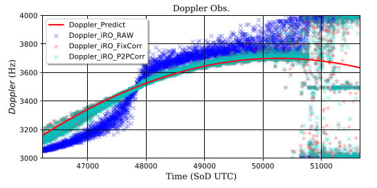
With $N_c=1000$, the estimated Doppler is presented in Figure 7, where it can be seen that the Doppler observations are inconsistent with the predicted Doppler, and the Doppler observations keep constant during the last period of the data collection (after SoD51000).

It is mentioned in [8] that the antenna beam should be narrow enough to avoid interferences from other GNSS transmitters. However, it can be seen from Figure 3 that a second satellite, i.e., SBAS PRN123 (ASTRA-5B), is also within the main beam of the antenna, and contributes significantly to the output of the auto-correlation in Equation (6). In the presence of two GNSS transmitters the auto-correlation function will be the sum of the auto-correlation functions of both transmitters. No cross-correlation term appears, because the PRNs of different transmitters are orthogonal to each other.

4.3.2. iRO Doppler Estimation with Removed Effect of PRN123

The presence of two different PRNs within the main beam of the antenna results in a phase pattern that cannot be attributed to a single PRN. The presence of the geostationary SBAS satellite results in constant phase and amplitude which are estimated using two distinct methods.

(1)

Fixed estimation: By assuming a constant amplitude, the contribution of PRN123 is estimated by averaging the correlation output in the period when PRN24 is out of the main beam of the antenna, i.e., after SoD51000.

$$\overline{{\mathbf{R}}_z^{\mathrm{PRN}123}}={〈{\mathbf{R}}_z〉}_{SoD>51000}$$

(18)

(2)

P2P correction: By assuming a non-constant amplitude, the contribution of PRN123 is corrected point by point (p2p) by the amplitude of the waveform obtained with the clean replica method, and the contribution of PRN123 to the output of the iRO cross-correlation can be estimated by

$$\begin{array}{c}\hfill {\mathbf{R}}_{z_{\mathrm{iRO}}}^{\mathrm{PRN}123}\left(t_1\right)=\overline{{\mathbf{R}}_{z_{\mathrm{iRO}}}^{\mathrm{PRN}123}}\frac{{\left|{\mathbf{R}}_{z_{\mathrm{CR}}}^{\mathrm{PRN}123}\left(t_1\right)\right|}^2-{\left|{\mathbf{R}}_{z_{\mathrm{N},\mathrm{CR}}}^{\mathrm{PRN}123}\left(t_1\right)\right|}^2}{{\left|\overline{{\mathbf{R}}_{\mathrm{CR}}^{\mathrm{PRN}123}}\right|}^2-{\left|\overline{{\mathbf{R}}_{z_{\mathrm{N},\mathrm{CR}}}^{\mathrm{PRN}123}}\right|}^2}\end{array}$$

(19)

in which $\overline{{\mathbf{R}}_{z_{\mathrm{CR}}}^{\mathrm{PRN}123}}$ is the clean-replica cross-correlation output averaged after SoD51000, ${\mathbf{R}}_{z_{\mathrm{CR}}}^{\mathrm{PRN}123}\left(t_1\right)$ is the the clean-replica cross-correlation output at $t_1$, the subscript $\mathrm{N}$ denotes the thermal noise component, and the noise components $\left|{\mathbf{R}}_{z_{\mathrm{N},\mathrm{CR}}}^{\mathrm{PRN}123}\left(t_1\right)\right|$ and $\left|{\mathbf{R}}_{z_{\mathrm{N},\mathrm{CR}}}^{\mathrm{PRN}123}\left(t_1\right)\right|$ are computed from the signal free area, i.e., 2 chips before the peak of the waveform.

The contribution of PRN123 estimated with both methods is then removed from the cross-correlation output, and the Doppler of the received signal can be estimated again.

The Doppler estimations by applying both inter-satellite interference removing methods are presented in Figure 8. It can be seen that the Doppler observation with the iRO technique is consistent with the predicted one by removing the contribution of PRN123.

Table 1. Standard deviation of the estimated Doppler respect to the predicted one in two different time periods.

SoD	<48,000	48,000–50,600
iRO Raw	79.0 Hz	30.5 Hz
iRO with Fixed Correction	19.9 Hz	10.4 Hz
iRO with P2P Correction	22.4 Hz	11.1 Hz

shows the standard deviation of the estimated Doppler with respect the predicted one, for two periods of time. The corrected iRO method is unable to provide correct Doppler estimates towards the end of the experiment (SoD $>\mathrm{50,600}$), when the SNR is lowest. But just before, it is when the correction works best.

In this situation, the Doppler frequency of PRN24 is large, and the Doppler filtering caused by the phase-compensated autocorrelation in Equation (11) is very effective in removing any residual contribution of PRN123, who has a zero Doppler because it is a geo-stationary satellite. At the beginning of the experiment, when PRN24 is at higher elevation, its Doppler frequency is smaller, and the Doppler filtering of other PRNs with similar (or zero) Doppler is not so effective. In the case of a spaceborne RO receiver the Doppler dynamics are much larger than in a ground-based experiment as the one presented in this paper. This means that the phase-compensated autocorrelation will allow to provide better Doppler filtering in a spaceborne receiver than in a ground-based experiment.

The results obtained with both correction methods are very similar, so the result from the fixed correction method is used in the following analysis.

4.3.3. SNR Analysis

The precision of Doppler estimation relies on the SNR of the interferometric waveform. In Figure 9, the evolution of the SNR is presented together with the elevation and the iRO Doppler estimation. The SNR for the clean-replica processing has been obtained with an integration time of 1 ms, while for the iRO processing the measurements have been further integrated to 1 s. Thus the vertical scale on the plots shows such a big difference for both types of measurements. It is worth to mention that the SNR of the received signal shows strong dispersion between SoD48000 and SoD50600 with the elevation between ${17}^{\circ }$ and $0^{\circ }$. That could be explained by the interference from the sea surface reflected signal which causes fading of received signal. At grazing geometries the polarization of the reflected signal is mainly at the same RHCP polarization as the direct signal.

From [14], the SNR of the interferometric waveform $SN{R}_{INT}$ can be expressed as

$$SN{R}_{INT}=\frac{T_C^{INT}}{T_C^{CR}}\frac{SN{R}_{CR}}{1+\frac{1+SN{R}_{PRE}}{SN{R}_{PRE}}}=\frac{T_C^{INT}}{T_C^{CR}}\frac{SN{R}_{CR}}{2+\frac{1}{SN{R}_{PRE}}}$$

(20)

where $SN{R}_{CR}$ is the SNR of the clean-replica open loop waveform, $SN{R}_{PRE}$ is the SNR at the input of the correlator, $T_C^{CR}$ is the coherent integration time of the clean replica waveform and $T_C^{INT}$ is the coherent integration time of the interferometric waveform. The quotient of the different integration times serves to take into account the different integration times for the clean replica and interferometric observables.

Given the bandwidth of the received signal B, we have

$$SN{R}_{CR}=B·T_C^{CR}·SN{R}_{PRE}$$

(21)

With Equations (20) and (21), the relationship between the clean replica and interferometric SNRs can be derived as

$$SN{R}_{INT}=\frac{T_C^{INT}}{T_C^{CR}}\frac{SN{R}_{CR}}{2+\frac{B·T_C^{CR}}{SN{R}_{CR}}}$$

(22)

Given the parameters in this signal processing: $B=2$ MHz, $T_C^{INT}=1$ s and $T_C^{CR}=1$ ms, the theoretical relationship between the clean replica SNR and the interferometric SNR is presented in Figure 10 with a continuous line. It can be seen that the relationship between $SN{R}_{CR}$ and $SN{R}_{INT}$ from the measured data is consistent with that derived theoretically.

In addition, the fact that the data points follow the shape of the line is indicating that the SNR variations in Figure 9 are the same for the clean replica and interferometric methods, and are thus not random noise, but correspond to actual fading which is consistently observed with both methods.

The actual SNR data plotted in Figure 10 is 2.78 dB (mean value) below the theoretical model, indicating that $SN{R}_{INT}$ is lower than expected. A possible explanation to this could be the fact that the raw data has been acquired with 1-bit quantization, which induces a degradation of SNR. However, such degradation has not been taken into account in Equation (22).

According to [15] the computation of the cross-correlation of one bit quantized Gaussian noise suffers a SNR loss of $2/\pi =0.637$, which corresponds to 2 dB. Although in the PARIS Interferometric Technique this is not strictly the case (non-Gaussian signal, low SNR), we assume that both situations are comparable.

We have to remark that [15] defines the SNR at the output of the correlator as the quotient formed by the mean value of the correlator output and the standard deviation of the correlator output. But other authors as [16] or [14] define the SNR at the output of the correlator as the quotient between the mean squared value of the correlator output and the variance of the correlator output. Thus, the latter definition of SNR is obtained by squaring the former one. In this case we translate the linear SNR loss of $2/\pi$ to the square SNR loss ${(2/\pi )}^2$, which is about $-3.9$ dB.

For the clean replica case we use [17] where the computation of a matched filter using quantized signals is studied. In this case the SNR definition at the output of the correlator is equivalent to the one in [16], although it is expressed in terms of $E_b/N_0$. Our receiver has a bandwidth of approximately B = 40 MHz, the chip $T_{CA}$ duration is approximately $1\mathsf{\mu }$s for CA code. The sampling frequency is $F_s=80$ MHz, which corresponds to 40 samples per chip. Using the tables given in that paper with:

$$\begin{array}{ccc}\hfill B{T}_{CA}& =& 40>10\hfill \\ \hfill f_{s_{CA}}& =& 2B{T}_{CA}\hfill \end{array}$$

where $f_{s_{ca}}$ is the number of samples per chipping symbol, the degradation due to quantization is in the order of $D_Q=-2.1$ dB.

This means that the degradation due to quantization in the interferometric technique respect to the clean replica is about $-3.9$ dB − ($-2.1$ dB) = −1.8 dB worse. When the one-bit quantization is taken into account, the SNR comparison is more consistent, and the bias has been reduced to 0.98 dB (see Figure 11).

The precision of the iRO measurement depends on the SNR at the auto-correlation output. In Figure 12, the precision of the measured Doppler is presented as a function of the SNR of the cross-correlation output. The Doppler precision is computed from the difference between the time series of measured Doppler and a simple fitted piecewise linear function every 10 s, and the SNR is also averaged in the same period. It is clearly shown that the precision of the Doppler measurement improves with the increasing of the SNR.

4.3.4. Zenith iRO Processing

In [8], an alternative approach to interferometric radio occultation is also proposed, in which the reference signal is acquired before any occultation actually happens, with the objective to increase the SNR of the occultation cross-correlation. We took the reference signal at SoD48000 when the antenna gain and the SNR were high enough and the received signal did not suffer serious interference from the sea surface reflection. The signal processing for the zenith iRO consists the following steps:

(1)

Reference signal acquisition: A signal segment of 20 ms ($s_{\mathrm{r}}^{\mathrm{ref}}\left(t\right)$) was selected from the data file corresponding to SoD48000, the starting sample of $s_{\mathrm{r}}^{\mathrm{ref}}\left(t\right)$ is aligned to the beginning of the navigation bit, which is estimated using the clean replica processing. It is worth to mention that the information on the navigation bit can be also predicted by the transmitter and receiver geometry when implemented in future space-borne interferometric receivers.

(2)

Down-conversion and coherent averaging: The selected signal segment was then down-converted to baseband by the local generated carrier with the predicted Doppler as

$$s_{\mathrm{r},\mathrm{BB}}^{\mathrm{ref}}\left(t\right)=s_{\mathrm{r}}^{\mathrm{ref}}\left(t\right)e^{-j2\pi f_{\mathrm{D},\mathrm{predict}}}$$

(23)

Then, 20 1-ms segments ($s_{\mathrm{r},\mathrm{BB}}^{\mathrm{ref}}(t_0+k/1000),k=0,1,\dots 19$) are cropped from the down-converted signal and coherently averaged as

$$s^{\mathrm{ref}}\left(t\right)={\displaystyle \sum _{k=0}^{19}}{s}_{\mathrm{r},\mathrm{BB}}^{\mathrm{ref}}(t_0+k/1000)$$

(24)

(3)

Open-loop tracking with the zenith reference: With the coherently averaged reference signal, a similar processing scheme from Section 4.2.2 is applied to the collected signal. It is noted that the initial code phase of the reference signal is also adjusted for each cross-correlation following the predicted Doppler by shifting the reference signal accordingly. The number of samples adjusted can be computed by

$$n_{\mathrm{sample}}^{\mathrm{incr}}\left(T\right)=\frac{f_{\mathrm{D},\mathrm{predict}}\left(T\right)T_i{F}_s}{f_{\mathrm{L}}1}$$

(25)

Following the processing scheme above, the Doppler of the received signal is estimated with the zenith iRO method and presented in Figure 13 together with the one estimated through the clean replica open loop processing. In Figure 14, both Doppler observations are compared in detail for two different typical periods with high and low SNRs. It can be seen from both figures that the zenith iRO Doppler observations are almost identical compared to those estimated with the clean replica method at higher elevations, when the SNR is larger. At higher elevations the performance in terms of RMS deviation of the observables respect to the predicted Doppler is almost identical, as shown in

Table 2. RMS deviation of the Doppler estimates respect to the predicted Doppler.

SoD	<48,000	48,000–50,600	>50,600
CR_OL	1.31 Hz	0.87 Hz	4.61 Hz
Zenith iRO	1.31 Hz	0.89 Hz	4.26 Hz

. At lower elevations, towards the end of the experiment, appreciable minor differences between both retrievals can be appreciated (see Table 2). It is worth to note, that the RMS values have been computed taking the predicted Doppler as a reference, and that in RO geometry the purely geometric predicted Doppler does not correspond to the real Doppler, as the atmospheric effects have not been modelled. Thus, the resulting RMS values could be affected by this mismodelling. We think that both methods are comparable in performance, and that the slight differences between the noise in both methods could be attributed to the fact that the reference signal used in the cross-correlation computation is different in both approaches. In the clean-replica method the received signal is cross-correlated with an ideal model of the GNSS signal, i.e., a perfect PRN sequence. When using the Zenith iRO method the received signal is correlated with a segment of the same signal acquired at a different instant of time, and thus, it includes all nuisances introduced by the GPS transmitter and receiver, such as filtering and other non-idealities, which are also common to the occulting signal segment. Consequently, the reference signal in the Zenith iRO would be better matched to the occulting signal than the ideal PRN sequence. This might explain the slightly better performance of the Zenith iRO technique compared to the clean-replica open loop processing. This conclusion should be taken with caution, as only one experimental evidence has been collected.

4.3.5. Effect of the Local Oscillator Frequency Offset

From Figure 14 (top), it can be noticed that although the Doppler estimates follow the predicted Doppler, they present small frequency jumps every 60 s. These frequency jumps can be observed in all the acquired data, and this particular data segment has been selected to zoom in, as it is representative of the acquired data. The reason for such jumps is that the receiver adjusts the local oscillator (LO) periodically to steer it towards its nominal frequency. These frequency jumps do not have any effect in the iRO technique computed at 1 ms delay, but in the Zenith iRO case, where the reference signal was acquired at a different time and with a slight different local oscillator frequency, this reflects into the phase measurement. As shown in Appendix A the Doppler frequency offset is given by

$$\Delta f_{\mathrm{d}}=-f_{\mathrm{off}}$$

(26)

for the Zenith iRO case. The SPIR receiver, that we used to record the data, also measures and records the actual reference clock from which the local oscillator is coherently derived. So we have a precise knowledge of the local oscillator frequency at any instant of time. Figure 15 shows corrected Doppler measurements for the same data segment as in the top plot in Figure 14. It can be appreciated that the jumps on the Doppler estimates have been corrected using Equation (26), and that the Doppler frequency evolves more smoothly.

5. Conclusions

In this work we have presented experimental results of the interferometric Radio Occultations technique (conventional and with reference signal acquired at Zenith) to measure the Doppler frequencies of GNSS signals, and compared the results with the ones obtained with other processing techniques, such as closed-loop and open-loop tracking using the clean replica.

We have seen that the conventional iRO technique is easy to implement in terms of signal processing needs, but suffers from inter-satellite interference due to the relatively large antenna beam width. In our experiment the interference was from a SBAS satellite at GEO orbit with nearly constant amplitude and Doppler, which we were able to estimate and remove from the correlation outputs in post processing. After the inter-satellite interference mitigation, the Doppler of the received signal has been estimated showing good agreement with its prediction. In terms of system architecture, implementing a receiver that employs the iRO technique requires highly directive, and thus large, antennas.

The precision of the iRO Doppler estimation depends on the SNR at the output of the cross-correlator. The relationship between the clean replica SNR and the interferometric SNR is analyzed and validated with the measured data. This analysis enables to model analytically the performance of the iRO technique in future space-borne GNSS remote sensing missions under different orbital and instrumental configurations.

In the demonstration of the zenith iRO technique, the reference signal was obtained when the SNR was high enough and the received signal did not suffer serious interference from the sea surface reflection. Moreover, the reference signal was averaged coherently before the cross-correlation to improve SNR, which can be also used in the space-borne scenario in case the antenna gain is not high enough. Also the effect of the local oscillator frequency offset on the observed Doppler estimation has been modeled analytically and successfully applied to the experimental data. After the comparison with the results obtained with the conventional clean replica open-loop processing, it is proved that the zenith iRO technique can achieve similar performance as the conventional approach. These results are relevant to potential future missions implementing interferometric GNSS reflectometry, such as the ESA PRETTY mission, enabling complementary iRO measurements using the same architecture.

References

- Jin, S.; Cardellach, E.; Xie, F. GNSS Remote Sensing; Springer: Berlin/Heidelberg, Germany, 2014; ISBN 978-94-007-7481-0. [Google Scholar] [CrossRef]
- Healy, S.; Jupp, A.; Marquardt, C. Forecast impact experiment with GPS radio occultation measurements. Geophys. Res. Lett. 2005, 32. [Google Scholar] [CrossRef]
- Cucurull, L.; Derber, J. Operational implementation of COSMIC observations into NCEP’s global data assimilation system. Weather. Forecast. 2008, 23, 702–711. [Google Scholar] [CrossRef]
- Anthes, R. Exploring earth’s atmosphere with radio occultation: Contributions to weather, climate and space weather. Atmos. Meas. Tech. 2011, 4, 1077. [Google Scholar] [CrossRef]
- Khaykin, S.M.; Funatsu, B.M.; Hauchecorne, A.; Godin-Beekmann, S.; Claud, C.; Keckhut, P.; Pazmino, A.; Gleisner, H.; Nielsen, J.K.; Syndergaard, S.; et al. Postmillennium changes in stratospheric temperature consistently resolved by GPS radio occultation and AMSU observations. Geophys. Res. Lett. 2017, 44, 7510–7518. [Google Scholar] [CrossRef]
- Lyu, H.; Hernández-Pajares, M.; Monte-Moreno, E.; Cardellach, E. Electron Density Retrieval From Truncated Radio Occultation GNSS Data. J. Geophys. Res. Space Phys. 2019, 124, 4842–4851. [Google Scholar] [CrossRef]
- Cardellach, E.; Oliveras, S.; Rius, A.; Tomás, S.; Ao, C.O.; Franklin, G.W.; Iijima, B.A.; Kuang, D.; Meehan, T.K.; Padullés, R.; et al. Sensing Heavy Precipitation With GNSS Polarimetric Radio Occultations. Geophys. Res. Lett. 2019, 46, 1024–1031. [Google Scholar] [CrossRef]
- Martín-Neira, M. GNSS interferometric radio occultation. IEEE Trans. Geosci. Remote Sens. 2016, 54, 5285–5300. [Google Scholar] [CrossRef]
- Høeg, P.; Fragner, H.; Dielacher, A.; Zangerl, F.; Koudelka, O.; Høeg, P.; Beck, P.; Wickert, J. PRETTY: Grazing altimetry measurements based on the interferometric method. In Proceedings of the 5th Workshop on Advanced RF Sensors and Remote Sensing Instruments, Noordwijk, The Netherlands, 12–14 September 2017. [Google Scholar]
- Ribó, S.; Arco-Fernández, J.; Cardellach, E.; Fabra, F.; Li, W.; Nogués-Correig, O.; Rius, A.; Martín-Neira, M. A Software-Defined GNSS Reflectometry Recording Receiver with Wide-Bandwidth, Multi-Band Capability and Digital Beam-Forming. Remote Sens. 2017, 9, 450. [Google Scholar] [CrossRef]
- Uhlemann, M.; Rudenko, S.; Nischan, T.; Gendt, G. GFZ results of the first IGS data reprocessing campaign. In Proceedings of the IGS Workshop, Newcastle, UK, 28 June–2 July 2010; Available online: ftp://stella.ncl.ac.uk/pub/IGSposters/Uhlemann.pdf (accessed on 21 November 2019).
- Kaplan, E.; Hegarty, C. Understanding GPS: Principles and Applications; Artech House: Norwood, MA, USA, 2005. [Google Scholar]
- Sokolovskiy, S.V. Tracking tropospheric radio occultation signals from low Earth orbit. Radio Sci. 2001, 36, 483–498. [Google Scholar] [CrossRef]
- Martin-Neira, M.; D’Addio, S.; Buck, C.; Floury, N.; Prieto-Cerdeira, R. The PARIS Ocean Altimeter In-Orbit Demonstrator. IEEE Trans. Geosci. Remote Sens. 2011, 49, 2209–2237. [Google Scholar] [CrossRef]
- Thompson, A.R.; Moran, J.M.; Swenson, G.W. Interferometry and Synthesis in Radio Astronomy, 2nd ed.; Wiley: Hoboken, NJ, USA, 2004. [Google Scholar]
- Proakis, J.G.; Salehi, M. Communication Systems Engineering; Prentice-Hall International, Inc.: Upper Saddle River, NJ, USA, 1994; ISBN 0-13-095007-6. [Google Scholar]
- Chang, H. Presampling filtering, sampling and quantization effects on the digital matched filter performance. In Proceedings of the Eighteenth International Telemetering Conference, San Diego, CA, USA, 28–30 September 1982; pp. 889–915. [Google Scholar]
Sample Availability: The data collected can be downloaded from https://www.ice.csic.es/research/gold_rtr_mining/. |
Figure 1.
Delay of the signal at different instants of time.
Figure 2.
Diagram of the measurement setup.
Figure 3.
Visible GPS satellites at the experiment location and time. The approximate 3 dB main beam of the RO antenna has been plotted using a blue line. The dashed line corresponds to the part of the beam below the horizon. An azimuth mask (45–180) has been applied to the visible satellites.
Figure 4.
Elevation of PRN24 (a) and its predicted Doppler frequency (b). Only the receiver and transmitter geometry has been used to obtain the predicted Doppler, no atmospheric effects have been considered.
Figure 5.
Doppler frequency estimated with the carrier tracking loop.
Figure 6.
Doppler frequency estimated with open loop processing. (a) shows the complete measurement period. (b) zooms into the end period of the experiment when the transmitter was occulting.
Figure 7.
Doppler estimation of PRN24 with the iRO technique.
Figure 8.
iRO Doppler estimation for PRN24 with removed effect of PRN123.
Figure 9.
Evolution of SNR for both the clean replica processing and the iRO processing. (a) SNR using the clean-replica method. (b) SNR using the iRO method. (c) iRO Doppler estimation with fixed correction.
Figure 10.
Relationship between the clean replica SNR and the interferometric SNR.
Figure 11.
Relationship between the clean replica SNR and the interferometric SNR by considering the degradation due to quantization.
Figure 12.
Relationship between the SNR and the precision of the iRO Doppler observation.
Figure 13.
Comparison between the Doppler observations obtained with the zenith iRO approach and the clean replica open loop processing.
Figure 14.
Doppler observation obtained with the clean-replica open loop and Zenith iRO approaches in two different periods. Both methods have a comparable performance. Top: representative period with high SNR. Jumps in the Doppler estimates every 60 s due to the adjustment of the local oscillator frequency can be observed. Bottom: End period of the experiment with occulting transmitter.
Figure 15.
Doppler observation after the correction of the local oscillator frequency offset.