A Novel Method for Plane Extraction from Low-Resolution Inhomogeneous Point Clouds and its Application to a Customized Low-Cost Mobile Mapping System

Abstract

Over the last decade, increasing demands for building interior mapping have brought the challenge of effectively and efficiently acquiring geometric information. Most mobile mapping methods rely on the integration of Simultaneous Localization And Mapping (SLAM) and costly Inertial Measurement Units (IMUs). Meanwhile, the methods also suffer misalignment errors caused by the low-resolution inhomogeneous point clouds captured using multi-line Mobile Laser Scanners (MLSs). While point-based alignments between such point clouds are affected by the highly dynamic moving patterns of the platform, plane-based methods are limited by the poor quality of the planes extracted, which reduce the methods’ robustness, reliability, and applicability. To alleviate these issues, we proposed and developed a method for plane extraction from low-resolution inhomogeneous point clouds. Based on the definition of virtual scanlines and the Enhanced Line Simplification (ELS) algorithm, the method extracts feature points, generates line segments, forms patches, and merges multi-direction fractions to form planes. The proposed method reduces the over-segmentation fractions caused by measurement noise and scanline curvature. A dedicated plane-to-plane point cloud alignment workflow based on the proposed plane extraction method was created to demonstrate the method’s application. The implementation of the coarse-to-fine procedure and the shortest-path initialization strategy eliminates the necessity of IMUs in mobile mapping. A mobile mapping prototype was designed to test the performance of the proposed methods. The results show that the proposed workflow and hardware system achieves centimeter-level accuracy, which suggests that it can be applied to mobile mapping and sensor fusion.

1. Introduction

In the past decade, mobile indoor mapping has become an important global research area, and the development of as-built Building Information Modeling (BIM) has introduced new challenges in acquiring detailed shapes and textures of indoor environments. Various research teams and companies released their products in the form of trolleys [1,2,3], backpacks [4,5,6,7,8,9,10], and handheld devices [11,12,13]. Most of these products integrate one or more multi-line laser scanners with Inertial Measurement Units (IMUs) to implement Simultaneous Localization And Mapping (SLAM) algorithms for mapping in Global Navigation Satellite System (GNSS)-denied environments. These configurations generate point clouds of indoor environments by registering data frames, by matching and aligning the extracted features or the global distribution of points with the assistance of the acceleration data stream provided by the IMU [14,15,16]. Points and primitives, such as lines, planes, and cylinders, are used as features in the registration process to recover the changes in position and attitude [17,18,19]. However, the use of multi-line Mobile Laser Scanners (MLSs) as one of the main point cloud capturing sensors has the following drawbacks that may affect the application of conventional feature extraction methods.

(1) Low-resolution and inhomogeneous point distribution. For most of the data captured by Terrestrial Laser Scanners (TLSs), Airborne Laser Scanners (ALSs), profiler-based MLSs, and RGB-Depth (RGB-D) cameras, the point resolutions along different directions are relatively similar, although there might be variations due to changes in distance between the objects and the sensors, profiler rotation speeds, and platform moving speeds. In certain circumstances, the resolution of point clouds captured by ALSs and profiler-based MLSs might be quite low along the moving direction of the platform due to the changes in moving speed. The point clouds could be resampled as the overall point cloud are dense enough. For data captured by multi-line MLSs, the vertical angle interval is commonly several times the horizontal interval, such as 2° versus 0.1° on a Velodyne VLP-16 scanner, making the point distances between neighboring points along the vertical and the horizontal directions much different. The resampling operation is also not applicable in processing such point clouds as the number of points are already limited. This jeopardizes the reliability in applying conventional point processing methods [20]. Although such mobile scanners are capable of capturing hundreds of thousands of points per second, taking Velodyne VLP-16 which is capable of capturing 300,000 points per second as an example, the unknown motion between frames, which consists of only 15,000 points, requires the dedicated algorithm to extract features from the low-resolution point clouds.

(2) Curvature and shape changes in scanlines. The laser-detector pairs inside the multi-line MLSs are installed at fixed angular intervals [21]. This leads to curved horizontal scanlines that are similar to concentric circles [22,23], different from the shape of scanlines generated by ALSs, profiler-based MLSs, and RGB-D sensors. The changes in scanline shapes increase the directional differences between neighboring scanlines, generating more uncertainty in scanline-based surface-detection methods.

(3) High ranging noises. Compact MLSs, like the highly popular Velodyne VLP-16, do not preserve the level of accuracy of their predecessors, such as Velodyne HDL-32E and 64E. The long-term accuracy of VLP-16 is only ±3 cm [21], and it thus creates a range of results with high uncertainty. In scanline analysis processes, such as Douglas-Peucker or other line simplification process, large thresholds might be adopted in conventional filtering methods, and the small variations on object surfaces and the unidentified curvature changes might be ignored.

In this paper, we propose the Enhanced Line Simplification (ELS) algorithm to address these issues and to effectively and efficiently extract planes from such low-resolution inhomogeneous point clouds. The method utilizes the original data acquisition sequence of the MLS to recover point grids and apply the line simplification algorithm to generate line segments. Then, the presented method is used to cluster line segments to form planar patches with respect to the scanline directions. The patches are merged in the final step to eliminate over-segmentation created by measurement noise and inevitable scanline curvatures. This method avoids the estimation and comparison of local normals and generates satisfactory results given low-resolution inhomogeneous point clouds. To test the robustness of the ELS algorithm, a plane-to-plane point cloud alignment workflow was designed to simulate the SLAM process of indoor mobile mapping systems. The implementation of a coarse-to-fine strategy and a shortest-path initialization method eliminates the necessity of IMUs for indoor mobile mapping. As there are already some papers evaluating the performance of popular IMU-based mobile mapping systems and providing quantitative accuracy assessments [14,15,16,24], the results produced by the proposed system are compared with the point clouds captured by a TLS as reference and show acceptable accuracy in the settings of a laboratory, a lecture hall, a stairwell, and an outdoor terrace.

The paper is structured as follows: Section 2 reviews the related plane extraction methods and discusses their limitations. Section 3 presents the proposed method for plane extraction, and Section 4 discusses its applications to IMU-free registration workflow. Section 5 describes the sample datasets and processing results and then compares the proposed method to popular methods. A discussion is provided in Section 6. Finally, conclusions are given in Section 7.

2. Related Works

To better understand the geometric representation in 3D point clouds, point clouds are divided into groups in the segmentation procedure. Various segmentation methods, such as edge-based methods, region-based methods, attribute and feature-based methods, model-based methods, and hybrid segmentation techniques were introduced to detect and isolate primitives, such as planes, spheres, and cylinders [25,26]. Planes, which exist in both natural and human-made environments, are which among the most common primitives and are the most straightforward to model. In indoor settings, they can be used to represent the approximations of uneven surfaces. Various methods have been introduced to extract planes from point clouds captured by different kinds of sensors. For point clouds captured by TLSs, ALSs, and depth cameras, the even distribution of points does not constrain processing methods based on geometric distances and local neighborhoods. However, the points captured by profiler-based single-line and multi-line MLSs are anisotropic and inhomogeneous, requiring dedicated algorithms based on scanline analysis.

RANdom SAmple Consensus (RANSAC) and its variants are the most popular plane extraction methods for evenly distributed dense point clouds [27,28,29,30,31]. These methods iteratively check the random choice of subsets to fit the hypothetic models and select the one with the largest size. To facilitate the fitting residuals, the variants were designed to take the likelihood and weights into consideration to distinguish parallel planar neighbors [32,33]. However, RANSAC-based methods are easily affected by the irregular distribution of points, which occurs when there are substantial density differences. Excluding congested regions in the point cloud requires the use of local estimated normals, which are error-prone in point clouds with variable resolutions. The initial segmentation for detecting the first RANSAC plane is critical for the whole modeling process and is time-consuming [34], and the pre-segmentation of the point cloud would enhance its performance.

Alternatively, region growing methods are commonly used based on the introduction of normal vectors [35,36,37]. The distance to the nearest patch edge and the normal difference are used as parts of the growing criteria. Voxels were defined to improve efficiency and enhance robustness as well [38,39,40,41]. However, the region growing methods are sensitive to varying point sparsity. Varying point sparsity determines the search radius in the extension process, and the diverted normal estimations also affect the addition of edge points [31,42]. The initial voxel generation is critical because it determines the geometric characteristics of the local vicinity. The inability to identify voxels of elements with similar geometric characteristics results in feature detection failure. Although [41] introduced the multi-scale method, the results are not promising for polarized point clouds captured by multi-line MLSs and may not distinguish nearby objects. An alternative is to use the grid distribution of points in the normal estimation process, which does not consider the distance between neighboring rows or columns. This results in deflections in normal directions due to their long-distance neighbors, especially for the knee points on scanlines [43,44]. Such errors are critical for extracting planes consisting of two or three scanlines and may result in detection failure.

For inhomogeneous point clouds captured by 2D profilers and a 3D multi-line MLS installed on a moving platform, the difference in point density along the internal rotation direction and its perpendicular direction creates additional difficulties in applying the methods mentioned above. The search radius, which is used for estimating tangent planes and edge growing, needs to be determined carefully along each direction to adequately present the local characteristics. Therefore, the segmentation of single scanlines and their clustering is adopted widely in processing MLS point clouds. Neighboring scanline segments with similar pointing directions were clustered into the same group to form planar patches [45,46,47,48]. However, the methods only considered the data acquisition directions and were not reliable when processing noisy datasets in which the linear distribution might be disrupted by the significant disturbance of points along the scanline. The inevitable scanline curvatures may force the threshold for segmenting scanlines to a larger value, causing undetected disturbances grouped into the plane. An “over-fragmentation” problem might also occur because of such measurement noise. An extra fraction fusion would be required to apply this method to noisy datasets. Furthermore, [22] presented a method that utilized scanline curvatures as the identifiable features for detecting planes. However, the size of the planes, the length of the scanline segments, and the distance between the scanner and the scanline would greatly affect the significance of the curvatures and the successful detection of the planes.

To align overlapped point clouds captured at different positions, the coarse alignment and the fine alignment are involved: (a) point, linear or planar features are extracted in an automatic process; (b) a manual selection process is performed or an automatic matching progress utilizing the RANSAC strategy is implemented to match the primitives, solving the rotation matrix and the translation to provide a coarsely alignment, since the uneven distribution of features leaves residuals in the alignments; and (c) a fine registration process, which is usually based on Iterative Closest Point (ICP) algorithm, is conducted to achieve high-accuracy alignments [49,50,51,52,53]. However, the global ICP process would introduce new errors to the registration as the low-resolution and inhomogeneous distribution of points influences the iterative approximation results and generate misalignments.

For registering point clouds captured on dynamic platforms, the coarse alignment process is usually replaced by the introduction of hardware sensors, namely GNSS receivers and IMUs [53]. Points [35,54,55,56,57,58,59,60,61,62], lines [63,64,65,66], planes [23,47,67,68,69,70,71], voxels [72,73], and the selections of them [19,74,75,76] are used to recover the positioning and orienting changes in the dynamic process and achieve fine registration. Since the limited number of planes extracted and the poor quality of planes may result in failures in aligning low-resolution single-frame point clouds, a highly robust and reliable plane extraction method is required for highly dynamic mobile mapping in indoor environments.

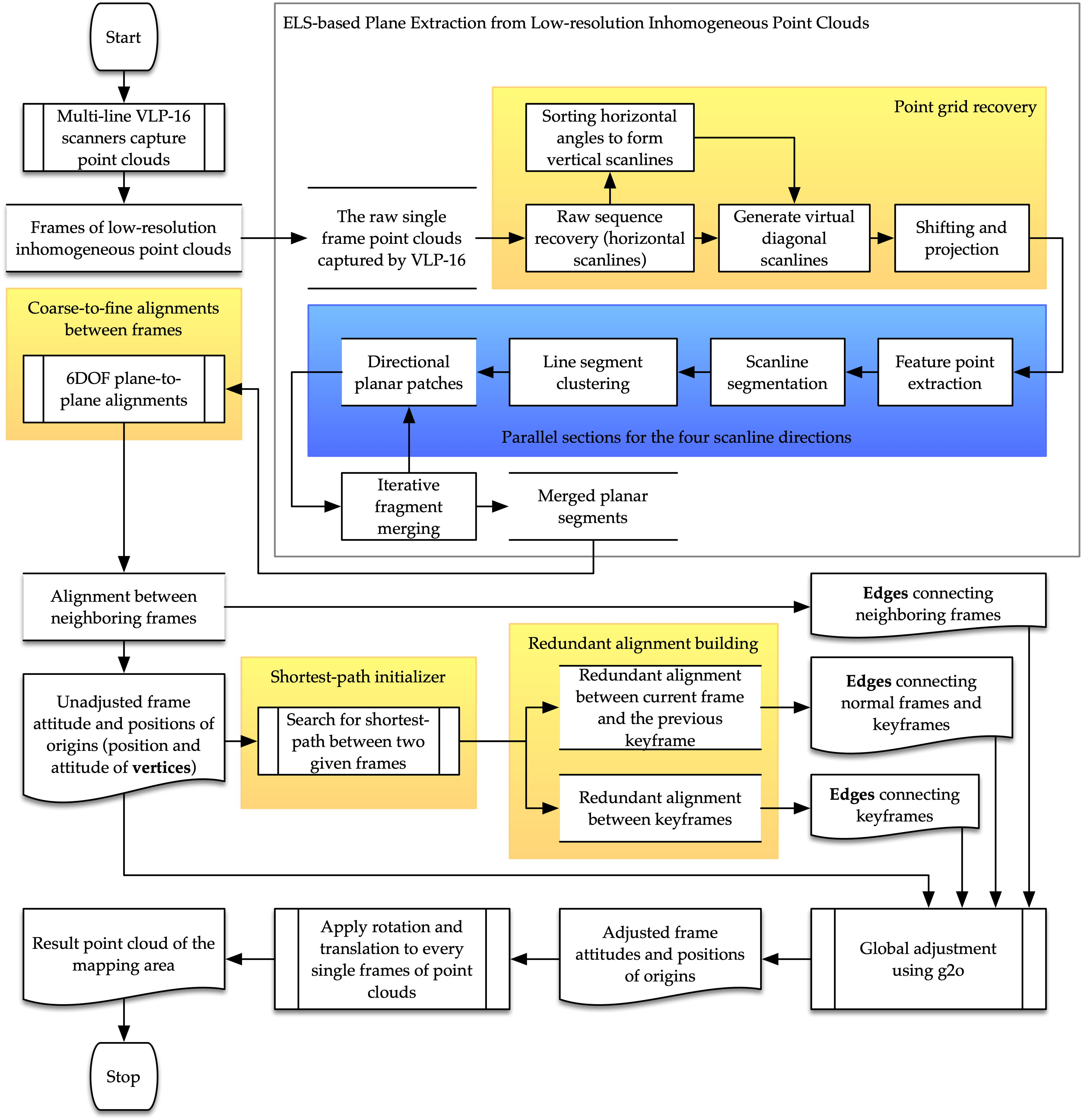
3. Plane Extraction Based on Enhanced Line Simplification Algorithm

The proposed plane extraction method based on the ELS algorithm is presented in this section with detailed steps. The initial procedure is the recovery of the original point grid, which is the virtual point cloud sequence in grid form, from the point clouds captured by the multi-line 3D MLS. Then, feature points are extracted using the line simplification algorithm concerning the scanline directions. Subsequently, the scanline segments are generated and clustered to form planar segments regarding the given scanline directions. Finally, planar patches of different groups are merged iteratively to form planes. Because the algorithm is designed to deal with the inhomogeneous point clouds, the data captured by the Velodyne VLP-16 are used to demonstrate the implementation of the proposed method to multi-line MLS point clouds. The general flowchart of the proposed method is shown in Figure 1.

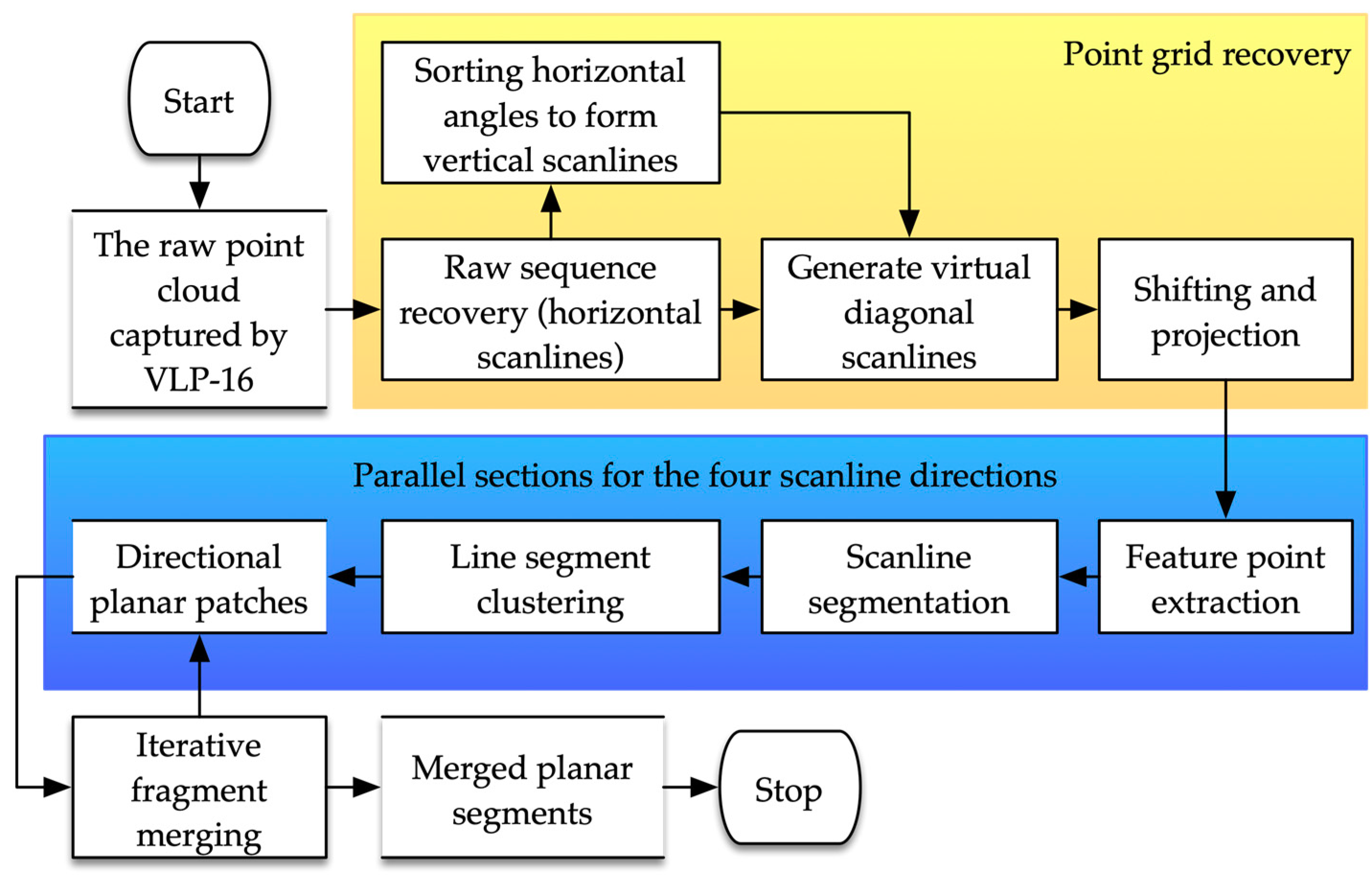
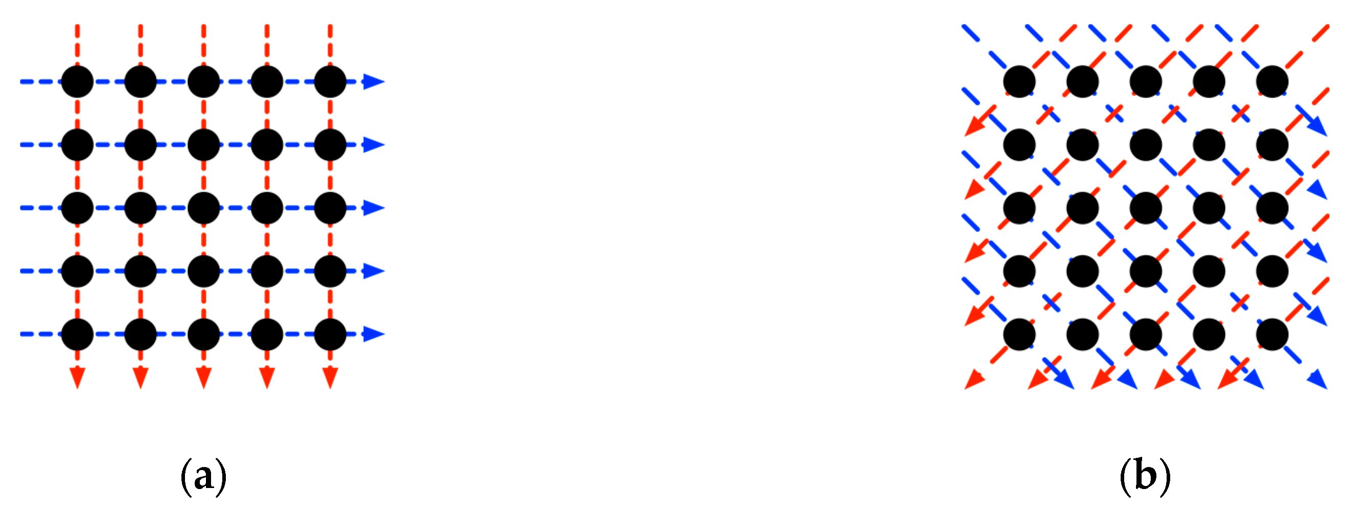
3.1. Point Grid Recovery

The first step of the entire ELS plane extraction workflow is the recovery of point grids representing the 2D distribution of points regarding the vertical and horizontal angles of the corresponding laser beams. The recovery process consists of the rearranging of points, scanline generation, shifting, and projection.

For most MLSs, the data capturing sequences are different from those of TLSs, in which the points in the same row or column share the same horizontal or vertical angles. Taking Velodyne VLP-16 as an example, the capturing sequence along the vertical direction does not strictly follow the ascending or descending order but an alternate sequence, as shown in Figure 2a. Therefore, the descending order must be recovered to form the sequential distribution of points in the vertical profile, making the line simplification applicable and concentrating on the sequential shapes of the polylines (Figure 2b). The offsets in horizontal angles, which are usually provided by the manufacturers, may also affect the rearranging of the points. For instance, on a RoboSense RS-LiDAR-32D 32-line MLS, the horizontal offsets between neighboring laser channels could be larger than 9.6″. This kind of back-and-forth distribution results in jagged changes in the horizontal angles, making the line simplification algorithm inapplicable along the vertical direction. Consequently, the points need to be rearranged concerning the individual horizontal angles in the form of the nearest neighbor search between laser beams. After the sequences along both the horizontal and vertical directions have been rearranged, the point cloud of a single frame can be filled into a grid network and is ready for the generation of the scanlines.

Because the scanner core is rotating against the vertical axis with the 16 beams, the horizontal scanline could be directly recovered, as in [46,47,48]. Nevertheless, in such implementations, only the variations along the single scanline direction were considered. Therefore, three virtual scanlines are introduced in the proposed method to enhance the feature point extraction process. As shown in Figure 3a, the vertical scanline corresponds to the rearranged sequence of the points in the same column because the points in the same vertical scanline share the same or similar horizontal angle. Due to the rotation of the scanner axis and the sequential emission of laser beams, the scanlines formed by the points in the same column are not precisely perpendicular to the horizontal scanline. They are named “vertical scanline” to indicate their functions in forming the point grids. With the horizontal and vertical scanline identified, the two diagonal directions of the grid cells are considered as the direction of the two virtual diagonal scanline directions, forming the scanlines shown in Figure 3b.

Shifting and projection are performed to eliminate shape changes in the perpendicular direction of the scanline plane. Such variations result from the actual shape changes, the fixed or unfixed horizontal offsets, and the variations of the internal rotation speed. In other words, the proposed method removes the components along the perpendicular directions to concentrate on the polyline shape changes within the plane formed by the two endpoints of the scanline and the origin of the scanner. In certain circumstances, points might be missing because the distance between the object and scanline might be out of the measurement ranges. Therefore, the neighboring points beside the missing point would be considered the endpoints of the scanline, as shown in Figure 4.

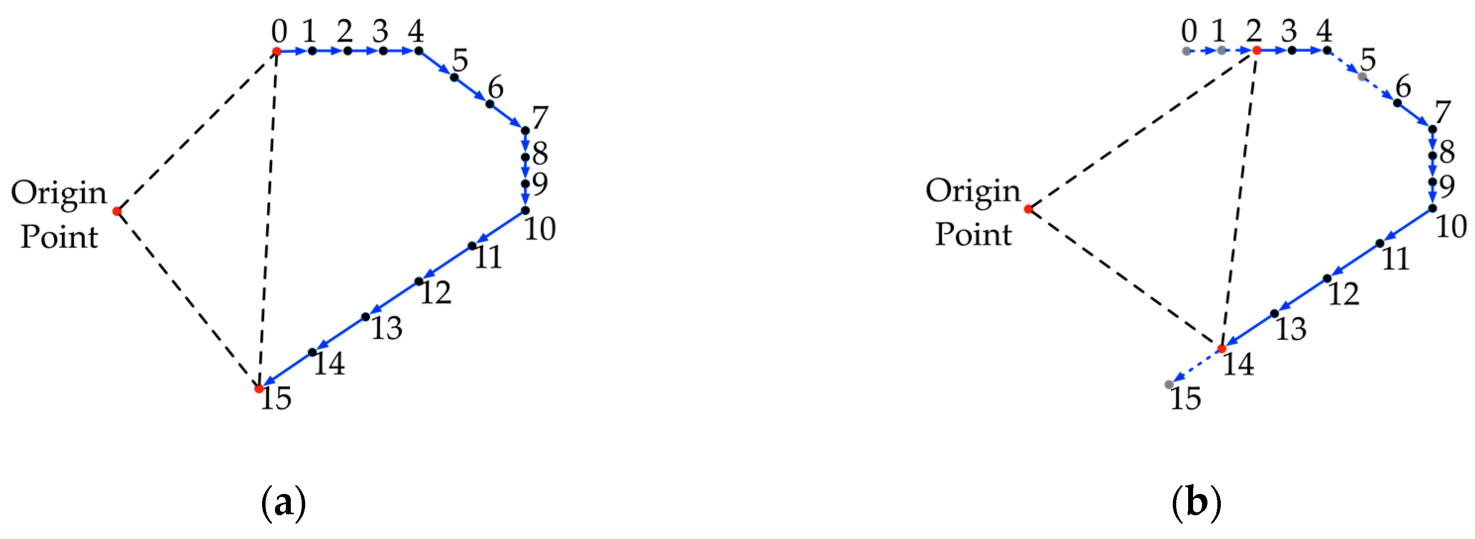
3.2. Feature Point Extraction

After all of the above preprocessing is conducted, the point grid is fully recovered, and the line simplification algorithm can be performed to extract the feature points to be used for plane extraction from such point clouds. In the proposed implementation, the Douglas–Peucker algorithm [77] is applied along the aforementioned four scanline directions, namely the horizontal, the vertical, and the two diagonal directions, with the threshold of one-and-a-half times the measurement accuracy of the laser scanner, which is an empirical value determined in the tests. The corresponding feature points are extracted in this operation.

In addition, significant feature points, which are comparatively much farther from one neighbor than their other on the line segment due to the incident angle of the laser beams and the distribution of objects, are labeled as feature points. Also labeled as feature points are invalid points with the zero coordinates to be skipped in the following scanline segment seeking process.

3.3. Scanline Segment Seeking and Clustering

Based on the definition of feature points in the previous step, non-feature points are defined as the ordinary points that are not extracted as feature points in the previous step, while the fake feature points are the points that are extracted as feature points due to scanline curvatures, but are not protruding points on the planes.

With all feature points identified, the scanline segmentation is conducted along the corresponding scanline directions. All non-feature points between the two feature points are extracted as a single scanline segment, and the two adjacent feature points on the two ends are added as the endpoints of the line segment. The directions of the segments are then estimated using Singular Value Decomposition (SVD).

Neighboring scanline segments are clustered into the same group if their directions (${\mathit{v}}_{dir}$) are similar. Because the objective of this clustering is not only grouping neighboring segments pointing similar directions but also generating the initial patches, a displacement vector is defined to facilitate the clustering process. The displacement vector (${\mathit{v}}_{dis}$) is defined as the unit vector pointing to the centroid of the pending line segment from the centroid of the current line segment. If the pending line segment is on the same plane as the current cluster, the cross product of ${\mathit{v}}_{dir}$ and ${\mathit{v}}_{dis}$ should be parallel to the normal of the current patch in theory. The introduction of the displacement vector is used to avoid clustering the two neighboring segments, which are on two different planes, into the same patch, like the example shown in Figure 5a.

When fake feature points are incorrectly extracted from curved scanlines with segments on the same plane, the scanline is split into two neighboring sections. Figure 5b demonstrates that the neighboring segment on the neighboring scanline can be used as intermedia, to cluster the two segments on the same scanline into the same patch. However, when the positions of fake feature points are similar on the adjacent scanlines, over-fragmentation results (Figure 5c). This will be eliminated in the multi-direction merging process.

After all the segments checked and clustered, an M-estimator SAmple and Consensus (MSAC) process [78] is implemented to remove the unwanted noise and disturbance from the given candidates and estimated the parameters of the plane.

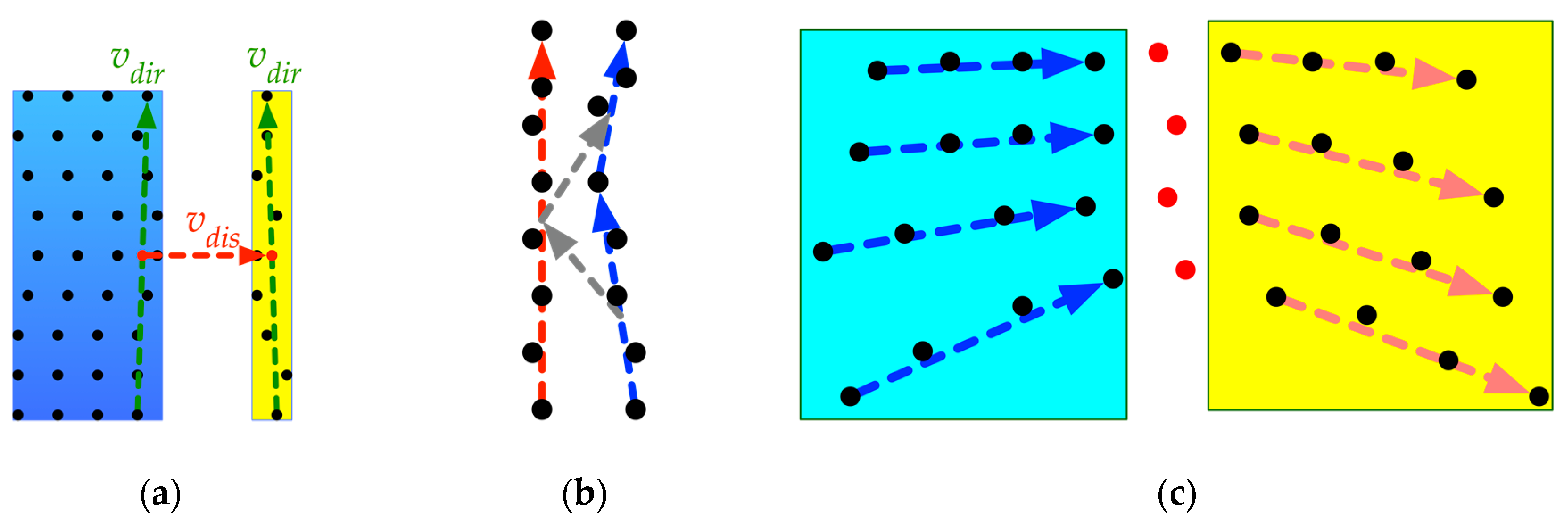
3.4. Multi-Direction Fragment Merging

Due to the unwanted scanline curvature changes and measurement noise, patches generated might be overly fragmented. The multi-direction merging process is conducted to combine the overlap fractions facing the same direction.

The merging process starts from iteratively comparing the normal directions of the two patches selected from different direction groups. Once identified as facing similar directions, the processor checks the existence of sharing points. Fractions are merged if there is at least one common point shared by patches because such a point must connect parts of the same plane. This iterative process continues until two patches selected from different direction groups cannot be merged because they do not share at least one common point. Consequently, the planes split by unwanted feature points in the previous step could be merged and the over-fragmentation problem is solved.

To address the problem of false merging, the number of fragment appearances in different groups are also checked. Only planes that are identified in more than two different direction groups are considered valid. The parameters of the plane are updated using MSAC, and possible noise and disturbance are removed as well.

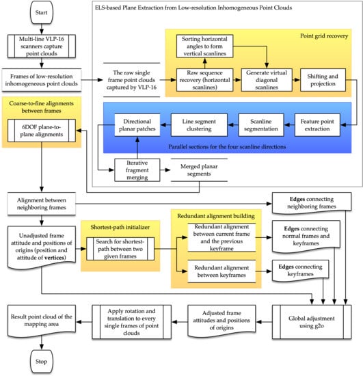
4. Applications to Mobile Mapping

A mobile mapping process was designed to demonstrate the application of the proposed ELS algorithm. In this process, the point clouds are aligned to the same reference frame to recover the geometric relationship between frames and restore the point positions in the unified reference system. In the proposed workflow, the alignment process is performed in a coarse-to-fine routine based on plane-to-plane alignments between frames. A single successful alignment between frames is named an observation, while the frames with significant changes from the last significant frame are called keyframes. Redundant observations are built between frames following the last keyframes, while the possibility of observations between every two keyframes is also explored and added as redundant observations, similar to the alignment strategy in [79].

4.1. Individual Alignment between Frames

Rotation matrices are used to describe the observations between point clouds. Therefore, given the point clouds of frame $i$ and $j$, the relationship between them is

$${\mathit{X}}_j^i=\mathit{R}{\mathit{T}}_{j\to i}^j{\mathit{X}}_j^j,$$

(1)

where ${\mathit{X}}_j^j$ and ${\mathit{X}}_j^i$ are the $4\times n$ matrices of point coordinates, namely ${\left[x y z 1\right]}^T$, representing the points of frame $j$ in the coordinate system of frame $j$ ($R_j$), which is the source frame, and frame $i$ ($R_i$), which is the target frame. $\mathit{R}{\mathit{T}}_{j\to i}^j$ is the $4\times 4$ transformation matrix that converts the point coordinates from $R_j$ to $R_i$. The proposed method uses the planes extracted from the low-resolution inhomogeneous point clouds captured by the Velodyne VLP-16 scanner to estimate the rotation and transformation matrix between the frames and align them to the same reference frame.

The correspondence between the planes of the source frames and the planes of the target frames need to be identified before the estimation of transformations. The alignment between two frames is coarsely initialized using either the corresponding motion between the two previous frames or the alignment determined by the Normal Distribution Transformation (NDT) [80,81]. With the estimated initial transformation provided, the plane pairs between frames are checked by calculating the vertical distance between parallel planes, the average density of points on the planes, the average Euclidean distances between any point pairs on the two planes, the portion of the overlap area, and the ratio of the number of points on the two planes. Then, the distribution of plane facing directions, in the form of a 3D vector of pairing score ($v_{PS}$), is checked in the estimation process to make sure the 6 degrees of freedom (6DoF) transformation can be estimated using the given plane groups. If the diversity of the plane facing direction cannot fulfill the requirement of forming three main directions, which are apart from each other, the plane-to-plane alignment cannot be performed, and the NDT results are used instead.

Once the correspondence between planes of source and target frames is defined and verified, the rotation and transformation between frames can be finely estimated using the plane-to-plane alignment. The non-linear process is implemented to detect the optimum rotation matrix for aligning the planes in $R_j$ to $R_i$ by minimizing the rotation residuals (${\epsilon }_{j\to i}^{Rot}$):

$$\min \left({\epsilon }_{j\to i}^{Rot}\right)={{\displaystyle \sum }}_k{\Vert 1-{\mathit{n}}_k^i·\left(\widehat{{\mathit{R}}_{j\to i}^j}{\mathit{n}}_k^j\right)\Vert }^2,$$

(2)

where ${\mathit{n}}_k^i$ is the normal direction of the plane $k$ in $R_i$, and $\widehat{{\mathit{R}}_{j\to i}^j}$ is the estimated rotation matrix from $R_j$ to $R_i$. Consequently, with the optimal rotation matrix, the transformation between the two frames is estimated by minimizing the transformation residuals (${\epsilon }_{j\to i}^{Transl}$):

$$\min \left({\epsilon }_{j\to i}^{Transl}\right)={{\displaystyle \sum }}_k{\Vert \left({\mathit{v}}_{k,j\to i}-\widehat{{\mathit{T}}_{j\to i}^{j,Rot}}\right)·{\mathit{n}}_k^i\Vert }^2,$$

(3)

where ${\mathit{v}}_{k,j\to i}$ is the vector between the centroid of the plane $k$ in $R_i$ and $\widehat{R_j^{j,Rot}}$, which is the rotated $R_j$ using the estimated rotation results in Equation (2), and $\widehat{{\mathit{T}}_{j\to i}^{j,Rot}}$ is the translation estimation based on the estimated rotation result.

Two weights are defined to introduce the quality of the plane correspondence into the estimation process. The first one is the ratio of the number of points on plane $k$ in $R_i$ to the corresponding value in $R_j$, which reflect the difference between the planes in point numbers. The other one is the ratio of the number of points on plane $k$ to the total number of points on planes in the same directional group.

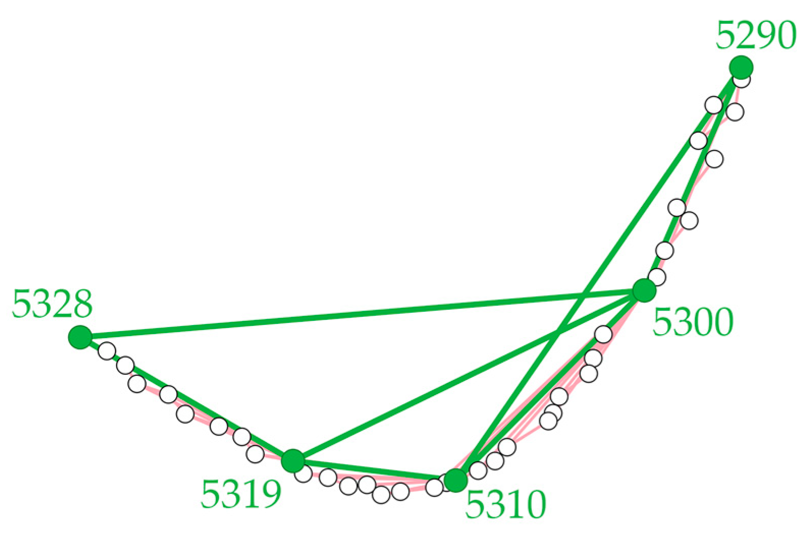
4.2. Overall Alignment Procedure

As the alignment errors propagate and increase in the recurrence process, there is a high possibility that the NDT operation may not provide valid initialization between distant frames. In most of the current systems, the IMU is integrated to provide the initialization between distant frames. However, the integration of an IMU increases the total cost of the system, while the IMU trajectory drifts with the quadratic integration of the acceleration [82,83]. In our solution, a redundant observation building process is implemented with a shortest-path initialization to waive the necessity of an IMU.

In addition to the alignment between adjacent frames, the redundant observation is built between non-adjacent frames. Therefore, when estimating the alignments between distant frames, the redundant observations forming the shortest path between them are used as the initial rotation and translation to reduce the drifting in the alignment propagation process. As in the example in Figure 6, multiple paths might be formed, and the one with the fewest edges is used as the selected path for transferring the rotation and transformation matrix from the source frame to the target frame for initializations. Consequently, the plane pairs are identified, and the precise rotation and translation matrices are estimated. In this process, the possible loops, such as the loop formed by frame 5300, 5310, 5319, and all frames between them in Figure 6, are also detected and established to form loop closure and reduce the accumulated drifting, produced in the frame-by-frame motion estimation process. This drifting is corrected in the final adjustment process.

In general, the overall point cloud alignment procedure consists of the individual alignments between adjacent frames, the normal-to-key observations between every frame and the nearest preceding keyframes, and the key-to-key observations between any two of the keyframes. All successful alignments are saved as edges connecting the two frames, and the initial positions and attitudes of frames are reserved as vertices. The corresponding primitives, namely the edges and the vertices, are imported into the General Graph Optimization (g2o) process [84], and the adjusted positions and attitudes are estimated.

5. Sample Datasets and Results

5.1. Plane Extraction from Low-Resolution Inhomogeneous Point Clouds

With the limitations of applying the popular plane extraction methods on the low-resolution point clouds captured by multi-line MLSs, most of the algorithms that use local normal estimations are not suitable for extracting patches. Like the examples shown in Figure 7b,c, the normals of points on a vertical wall are facing upwards or downwards because only points on the same horizontal scanline are within the local neighborhood determined by the inappropriate searching radius in normal estimation, while the disturbances and noises in distance measurements make the points distributed on a plane rather than the theoretical straight line. Consequently, most normal-based algorithms are affected. The region growing methods, which consider the local vicinity and the distance between points as the main factor in the extending process, are also affected by the varying distance between points, which changes with the distance between the objects and scanner. To demonstrate the advantages and disadvantages of the proposed methods, the methods introduced by [85] and [41] are used as reference methods in the comparison, as well as the classic RANSAC method [28].

Point clouds of multiple scenarios were captured and used to compare the results to demonstrate the capability of extracting certain kinds of planes. The testing scenarios include a hallway, which consists of low walls and a double-layer ceiling, a rectangular laboratory, a large lecture theater with a curved ceiling, and a narrow stairwell. All data were captured using a horizontally installed Velodyne VLP-16 multi-line MLS with 2° intervals between laser channels. The declared distance measurement accuracy of the scanner is ±3 cm [21]. Processing time for extracting planes are not considered as the metric for comparing the given methods, since the time used by every method is similar, while the concentration of the comparison is whether any of the method can produce reliable plane extractions. The results yielded a noticeable difference and are shown in

Table 1. The photos and illustrations of the raw point clouds ¹ and the plane extraction results using the RANSAC method [28], voxel cloud connectivity segmentation (VCCS) [85], multi-scale voxels [41], and the proposed method on the given data sets.

Scenario	Hallway	Laboratory	Lecture Theater	Stairwell
Photos
Raw Point Clouds
RANSAC 2
VCCS 3
Multi-scale Voxels 3
Proposed Method

¹ The raw point clouds are selected from data streams that captured on a dynamic platform during continuous mapping processes. ² The radius of the neighborhood in processing the lecture theater data was set to a much larger value (1.00 m) to form a reasonably large vicinity for estimating normals because the resolution between horizontal scanlines in that dataset varies from 0.10–2.00 m. ³ Only voxels are generated in the process, as an incorrect voxel will restrain the extraction of planes.

for visual comparison.

Generally, the proposed method produces the most reliable results compared to the three reference methods, especially in extracting planes of large open spaces with considerable resolution variation. Although the numbers of planes extracted by the proposed method are less than the plane extracted using other methods, the fragmented patches must be considered in the counting process as well. Therefore, planes that are unable to be extracted are also compared. With the parameters listed in [87] considered, the RANSAC implementation only produces acceptable results when given a proper radius for estimating local normals. However, points on a single scanline were considered as planar fractions (Figure 8a). The RANSAC method is not able to split the parallel objects properly and may consider them as the same object (Figure 8b). The voxel cloud connectivity segmentation (VCCS) method [85] generates voxels for dense regions correctly, while it creates voxels with single-line points when the distance between scanlines is significantly large (Figure 8c). Large or small voxel size must be set for processing certain regions, as there is no unified value. The multi-scale voxel introduced by [41], which was designed to solve the changeable voxel resolution problem in processing city-scale point clouds, created the most voxels correctly. The results are affected more by the local neighborhood than by the geometric characteristics (Figure 8d).

Additionally, some errors were categorized to show the difference clearly in

Table 2. The detailed comparison of the plane extraction results using the RANSAC [28] method, VCCS [85], multi-scale voxels [41], and the proposed method on given data sets. ^1.

Scenario	Unclear Edges	Stairs as a Slope	Single-Line Fractions	Undivided Fractions
RANSAC
VCCS 2
Multi-scale Voxels 2
Proposed Method 3

¹ For the results produced by RANSAC, VCCS, and Multi-scale Voxels methods, the planes and segments extracted incorrectly are marked with yellow boxes or arrows if not all of the results shown in the figure are wrong. For the results produced by the proposed method, only wrong extractions are marked in yellow boxes. ² Only voxels are generated in the process, as the incorrect voxel will prevent the extraction of planes. ³ There is no error in results of single-line fractions and undivided fractions using the proposed method.

. The common mistakes are categorized into four groups:

(1) Unclear edges. For the three reference methods, the local estimated normals are introduced as the geometric features of points and voxels. Therefore, when the normal directions are diverted, the extraction process cannot identify the edge accurately. In the RANSAC results, the edge points might be segmented as single planes given the number of points with diverted normals. For voxel-based methods, the wrong segmentation contributes to the voxel normals and require an extra modeling step to remove them. In the result produced by the proposed method, only a few points are wrongly grouped into the other plane because there is no normal required in the extraction process.

(2) Stairs as a slope. The stairs are connected Z-shaped regions that might be considered planes with noisy data. All four methods produce similar results in which all or some of the stairs cannot be distinguished. The RANSAC method extracts all of the points as a tilted plane in the experiment. Improvements have been made to reduce such errors, such as those by [32]. The VCCS method does not create voxels correctly, as the resolution between scanlines is low. The method of [41] fails to distinguish the stairs from each other and generates voxels consisting of multiple stairs. In contrast, the proposed method leans towards generating smaller segments, which are easier to identify and exclude.

(3) Single-line fractions. The resolution of the 3D MLS decreases with the increase in distance. For specific scenarios, such as open spaces, corridors, and tunnels, the distance between neighboring scanlines might be several meters. In the reference results, planes or voxels with only one scanline are generated, even for the multi-scale voxels. Voxels with only a single scanline might result in wrong normal estimations, leading to region growth failure. In contrast, the proposed method extracts planes successfully and can distinguish the parallel planes. It does not generate any single-line fractions because it requires at least one non-feature point as the seed and two additional endpoints in each of the four directions.

(4) Undivided fractions. For parallel planes with the distance of a few centimeters between their edges, the effective differentiation is also a challenge for the three reference methods. The VCCS method cannot generate valid voxels due to the considerable distance between the horizontal scanlines, while the RANSAC method and the method of Multi-scale Voxels method do not recognize the edge of the backrests and seats of the theater chairs. In contrast, the proposed method is capable of distinguishing the chairs but is only able to extract some of the planes correctly.

5.2. A Dedicated Mobile Mapping System, S²DAS

The plane-to-plane alignment workflow was applied to a dedicated mobile mapping solution, Seamless Spatial Data Acquisition System (S²DAS), developed. It consists of two multi-line Velodyne VLP-16 scanners, as shown in Figure 9. The distance between the scanners could be adjusted to fit the installation frames, and either a helmet or a backpack can be used as the installation platform. The angles between the two scanners are nearly 76°, making one of the scanners capturing point clouds of the surrounding environments horizontally while the other concentrates on capturing points bounced by the ceilings and floors. Therefore, planes facing multiple directions are extracted from point clouds captured by both the scanners. The alignment process facilitates the multiple facing directions of the extracted planes to determine the 6DoF movements between frames.

The leverarms between the two scanners are estimated using the common planes extracted from the two point clouds. In the calibration site, perpendicular planes are set in the overlapped Field-of-View (FOV) of the two scanners, as shown in Figure 10. Once the synchronization of the two scanners is achieved using a dedicated device that keeps simulating GNSS signals in indoor environments, the rotation and translation matrix between the two point clouds is estimated by manually aligning the planes extracted using the ELS algorithm.

In the implementations, the planes, which are separately extracted from either point clouds, were used to align the frames. In most of the cases, horizontal planes, such as ceilings and floors, and sidewalls on the left- and right-hand sides are more easily to be extracted from the point clouds captured by vertical scanner. Meanwhile, the extractions of sidewalls facing different directions are more straightforward, while the horizontal planes are not likely to be successful scanned and extracted. Consequently, all the planes extracted from both point clouds of single frame are used to estimate the attitude and position changes. However, only the points captured by the profiler were used to generate the final results, since the errors in attitude estimations are magnified by the larger distance between the points captured by the horizontal scanner.

5.3. Plane-to-Plane Alignments for IMU-free Mobile Mapping

The mobile mapping process was conducted in an empty lab (14.5 m × 16 m) to assess the accuracy of the point cloud (Figure 11a). Two movable blackboards were installed in the middle of the lab to facilitate the plane-based point cloud alignment process. Following [16], 152 rectangular targets were printed in A4 size, pasted on the four sidewalls and floor, and used as the targets for accuracy assessment. A FARO Focus M70 with the ranging accuracy of ±3 mm was used to capture the reference point clouds for comparison. The moving trajectory of S²DAS is illustrated in Figure 11b, while the generated point cloud and the distance measurement differences of the 11,476 edges are demonstrated in Figure 11c–f. The distance measurement results are compared with the TLS results, while the difference in distance measurements, fitting the normal distribution of $X~\mathcal{N}\left(0.24,9.54\right)$ and showing that a ±9.26 cm error in 99.7% of samples can be achieved. However, the accidental errors, which can be as large as 15.58 cm is also spotted, meaning there are still room for improvements in the future.

Table 3. The distance comparison statistics between the TLS point cloud and the S²DAS point cloud.

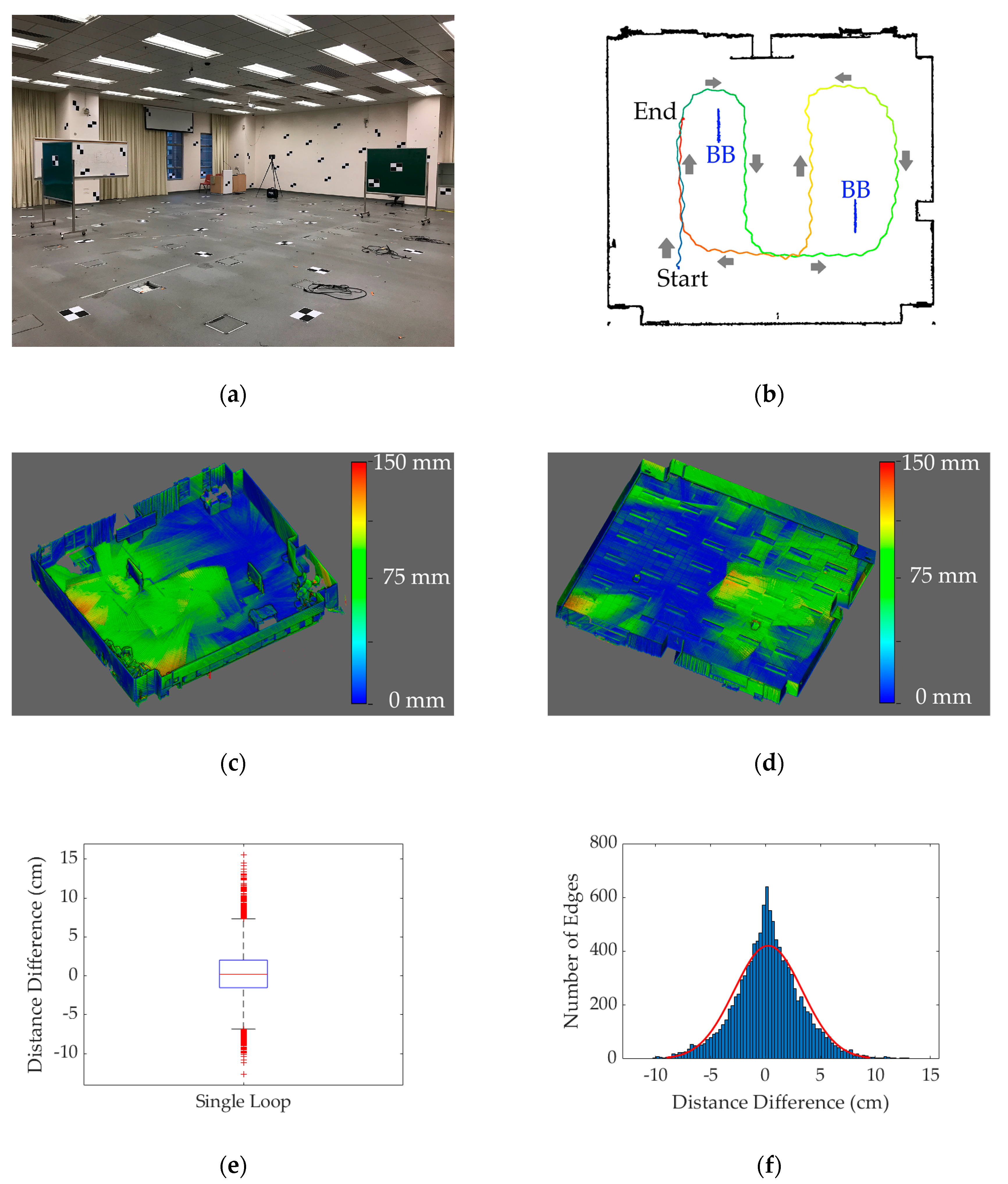
Error Type	Distance Measurement Error [cm]
Maximum Error	15.58
Minimum Error	−12.69
Mean Error	0.24
Standard Deviation	3.09
Root-mean-square Error	3.10

shows the detailed numerical statistics of the comparison [88,89,90,91,92]. The accuracy of the recovered trajectory is not considered as the assessment criterion, since the point distribution versus the TLS point cloud, the noise level of the point cloud produced, and the accuracy of the targets is capable of reflecting the accuracy level of the system, which is also the main requirement of applying such mobile mapping system.

In addition, verification experiments were conducted in complicated environments, including a lecture theater, a three-floor stairwell, and an outdoor terrace, as shown in

Table 4. The point clouds captured using FARO M70 TLS and S²DAS in complicated scenarios: a lecture theater, a stairwell, and an outdoor terrace.

Scenario	TLS Point Clouds 1	S2DAS Point Clouds 2
Lecture Theater 3
Stairwell 3
Terrace (outdoor)

¹ The TLS point clouds are colored using the RGB captured by the internal camera. ² The S²DAS point clouds are colored using the intensity value provided by the VLP-16 scanner. ³ The lecture theater and stairwell in this table are the same test sites as in Table 1.

. Details of the S²DAS point clouds are captured (Figure 12), showing that object shapes can be recovered correctly using the proposed IMU-free workflow.

6. Discussion

The proposed ELS-based method produces highly robust plane extraction results when processing low-resolution inhomogeneous point clouds. The methods used for comparison are affected by low distribution density when forming valid planes or voxels. Meanwhile, the variable sparsity in specific directions influences the estimation of the local normal, requiring a respective directional radius for defining local vicinity. Although the multi-scale method significantly improves results, extra steps might be required to eliminate possible errors. The proposed method overcomes the difficulty in searching for point neighbors by introducing the original data acquisition sequence and defining three additional virtual scanline directions. The normal estimation is not involved in the extraction process, reducing the computing load and significantly improving robustness regarding the low resolution and inhomogeneous issues. The analysis along the given directions removes unwanted details in scanline shapes while successfully maintaining the main characteristics. Furthermore, the proposed method combines the directional extraction results to eliminate the errors produced by fake feature points resulting from natural curvature changes. The comparison shows the proposed method produces significantly better results in processing point clouds with different sparsity in specific directions, which is common in multi-line MLS point clouds of large spaces. According to the given typical indoor scenarios, the proposed method performs better in generating more precise edges, distinguishing stairs, avoiding single-line plane fractions, and dividing plane fractions with minor separations.

Based on the proposed plane extraction method, a plane-to-plane alignment workflow is designed to achieve IMU-free mobile mapping. The result shows that in simple environments, the proposed method is capable of solving 6DoF alignments. Different from the traditional idea of using feature-based registration only in the coarse alignment process rather than accuracy fine alignment, the proposed method generates indoor mobile mapping results with centimeter-level accuracy. This accuracy is similar to IMU-based mobile backpack-based systems but lower than trolley-based solutions according to the given performance evaluation results in [14,16]. However, the testing environment in this paper is simple and planes are easy to identify. For complex environments where planes are not evenly distributed in multiple directions or not enough in any of the directions, the introduction of other positioning and orienting sensors, i.e. an IMU, will be essential.

7. Conclusions

This paper presents a plane extraction method with its application to 6DoF IMU-free mobile mapping. The plane extraction method utilizes the original data acquisition sequence of the point clouds with the introduction of virtual scanlines to facilitate a feature point extraction operation. Line segments are generated and clustered to form planar patches. The fractions of different directions are then merged to produce planes. The proposed method is compared with three popular methods and shown to be a better choice for low-resolution inhomogeneous point clouds captured by multi-line MLSs. Based on the proposed method, a plane-to-plane alignment workflow is introduced to realize the IMU-free mobile mapping in indoor environments. The coarse-to-fine strategy and the shortest-path initialization reduce the possibility of plane-to-plane alignment failure. Based on the proposed dual-MLS mobile mapping system, data were captured and processed. The system offers centimeter-level accuracy in test environments, and the results are used to produce 3D models [37].

However, the proposed method has limitations. The application of the ELS algorithm requires a pre-known data acquisition sequence of the point clouds and some of the specifications of sensors, those being the horizontal and vertical offsets of the laser channels, limiting its application to structured point clouds. The proposed system can only work in specific environments with planes facing multiple directions. If there are not enough planes or they are facing limited directions, the rotation and translation between the two frames cannot be estimated using the plane-only method. Therefore, the introduction of the IMU can enhance the reliability of the proposed system in complex environments, and it can be used as an alternative in such environments. Future work will include the application of the ELS algorithm to unstructured point clouds and the integration of the plane-to-plane alignment method with multiple positioning and orientation techniques, including but not limited to IMUs, GNSS receivers, and other SLAM methods.

8. Patents

The following patent arises from the work presented in this paper:

Shi, W. and Fan, W., Plane extraction method, system, device and storage medium based on point cloud data. P.R. China Patent application 201811167642.5.

References

- Applanix Corp. Land Solutions: TIMMS Indoor Mapping. Available online: http://www.applanix.com/solutions/land/timms.html (accessed on 8 December 2015).
- ViAmetris 3D Mapping Viametris|Continuous Indoor Mobile Scanner iMS3D. Available online: https://www.viametris.com/ims3d (accessed on 8 December 2015).
- NavVis US Inc. NavVis|M6. Available online: https://www.navvis.com/m6 (accessed on 12 April 2019).
- Leica Geosystems AG Leica Pegasus: Backpack-Award-Winning Wearable Reality Capture-Indoors, Outdoors, Anywhere. Available online: http://www.leica-geosystems.com/en/Leica-PegasusBackpack_106730.htm (accessed on 8 June 2015).
- Google Introducing Cartographer. Available online: https://opensource.googleblog.com/2016/10/introducing-cartographer.html (accessed on 5 October 2016).
- GreenValley International LiBackpack-Mobile Handheld LiDAR-3D Mapping System. Available online: https://greenvalleyintl.com/hardware/libackpack/ (accessed on 11 April 2019).
- ViAmetris 3D Mapping Viametris|Backpack Mobile Scanner bMS3D LD5+. Available online: https://www.viametris.com/bms3d4cams (accessed on 11 April 2019).
- Blaser, S.; Cavegn, S.; Nebiker, S. Development of A Portable High Performance Mobile Mapping System Using The Robot Operating System. ISPRS Ann. Photogramm. Remote Sens. Spat. Inf. Sci. 2018, IV–1, 13–20. [Google Scholar] [CrossRef]
- Nüchter, A.; Borrmann, D.; Koch, P.; Kühn, M.; May, S. A man-portable, IMU-free mobile mapping system. ISPRS Ann. Photogramm. Remote Sens. Spat. Inf. Sci. 2015, II, 17–23. [Google Scholar] [CrossRef]
- Liu, T.; Carlberg, M.; Chen, G.; Chen, J.; Kua, J.; Zakhor, A. Indoor localization and visualization using a human-operated backpack system. In Proceedings of the International Conference on Indoor Positioning and Indoor Navigation, Zürich, Switzerland, 15–17 September 2010. [Google Scholar]
- Occipital Inc. PX-80 Overview. Available online: http://labs.paracosm.io/px-80-overview (accessed on 16 July 2019).
- GeoSLAM GeoSLAM-The Experts in “Go-Anywhere” 3D Mobile Mapping Technology. Available online: https://geoslam.com/ (accessed on 11 April 2019).
- Kaarta Stencil 2–KAARTA. Available online: https://www.kaarta.com/products/stencil-2/ (accessed on 15 July 2019).
- Lehtola, V.; Kaartinen, H.; Nüchter, A.; Kaijaluoto, R.; Kukko, A.; Litkey, P.; Honkavaara, E.; Rosnell, T.; Vaaja, M.; Virtanen, J.-P.; et al. Comparison of the Selected State-Of-The-Art 3D Indoor Scanning and Point Cloud Generation Methods. Remote Sens. 2017, 9, 796. [Google Scholar] [CrossRef]
- Nocerino, E.; Menna, F.; Remondino, F.; Toschi, I.; Rodríguez-Gonzálvez, P. Investigation of indoor and outdoor performance of two portable mobile mapping systems. In Proceedings of the Videometrics, Range Imaging, and Applications XIV, Munich, Germany, 26–27 June 2017; Volume 10332I. [Google Scholar]
- Maboudi, M.; Bánhidi, D.; Gerke, M. Investigation of Geometric Performance of An Indoor Mobile Mapping System. ISPRS Int. Arch. Photogramm. Remote Sens. Spat. Inf. Sci. 2018, XLII–2, 637–642. [Google Scholar] [CrossRef]
- Zhang, Z. Iterative point matching for registration of free-form curves and surfaces. Int. J. Comput. Vis. 1994, 13, 119–152. [Google Scholar] [CrossRef]
- Zhang, J.; Singh, S. LOAM: Lidar Odometry and Mapping in Real-time. In Proceedings of the Robotics: Science and Systems (RSS), Berkeley, CA, USA, 13–17 July 2014. [Google Scholar]
- Olsson, C.; Kahl, F.; Oskarsson, M. The Registration Problem Revisited: Optimal Solutions From Points, Lines and Planes. In Proceedings of the 2006 IEEE Computer Society Conference on Computer Vision and Pattern Recognition (CVPR’06), IEEE, New York, NY, USA, 17–22 June 2006; Volume 1, pp. 1206–1213. [Google Scholar]
- Bogoslavskyi, I.; Stachniss, C. Fast range image-based segmentation of sparse 3D laser scans for online operation. In Proceedings of the 2016 IEEE/RSJ International Conference on Intelligent Robots and Systems (IROS), IEEE, Daejeon, Korea, 9–14 October 2016; pp. 163–169. [Google Scholar]
- Glennie, C.L.; Kusari, A.; Facchin, A. Calibration and Stability Analysis of the VLP-16 Laser Scanner. ISPRS Int. Arch. Photogramm. Remote Sens. Spat. Inf. Sci. 2016, XL, 55–60. [Google Scholar] [CrossRef]
- Grant, W.S.; Voorhies, R.C.; Itti, L. Finding planes in LiDAR point clouds for real-time registration. In Proceedings of the IEEE/RSJ International Conference on Intelligent Robots and Systems, Tokyo, Japan, 3–7 November 2013. [Google Scholar]
- Grant, W.S.; Voorhies, R.C.; Itti, L. Efficient Velodyne SLAM with point and plane features. Auton. Robots 2019, 43, 1207–1224. [Google Scholar] [CrossRef]
- Karam, S.; Vosselman, G.; Peter, M.; Hosseinyalamdary, S.; Lehtola, V. Design, Calibration, and Evaluation of a Backpack Indoor Mobile Mapping System. Remote Sens. 2019, 11, 905. [Google Scholar] [CrossRef]
- Vosselman, G. Point cloud segmentation for urban scene classification. ISPRS Int. Arch. Photogramm. Remote Sens. Spat. Inf. Sci. 2013, XL-7/W2, 257–262. [Google Scholar] [CrossRef]
- Nguyen, A.; Le, B. 3D point cloud segmentation: A survey. In Proceedings of the 2013 6th IEEE Conference on Robotics, Automation and Mechatronics (RAM), IEEE, Manila, Philippines, 12–15 November 2013; pp. 225–230. [Google Scholar]
- Fischler, M.A.; Bolles, R.C. Random sample consensus: A paradigm for model fitting with applications to image analysis and automated cartography. Commun. ACM 1981, 24, 381–395. [Google Scholar] [CrossRef]
- Schnabel, R.; Wahl, R.; Klein, R. Efficient RANSAC for Point-Cloud Shape Detection. Comput. Graph. Forum 2007, 26, 214–226. [Google Scholar] [CrossRef]
- Dimitrov, A.; Golparvar-Fard, M. Segmentation of building point cloud models including detailed architectural/structural features and MEP systems. Autom. Constr. 2015, 51, 32–45. [Google Scholar] [CrossRef]
- Xu, X.; McGorry, R.W. The validity of the first and second generation Microsoft KinectTM for identifying joint center locations during static postures. Appl. Ergon. 2015, 49, 47–54. [Google Scholar] [CrossRef] [PubMed]
- Dong, Z.; Yang, B.; Hu, P.; Scherer, S. An efficient global energy optimization approach for robust 3D plane segmentation of point clouds. ISPRS J. Photogramm. Remote Sens. 2018, 137, 112–133. [Google Scholar] [CrossRef]
- Xu, B.; Jiang, W.; Shan, J.; Zhang, J.; Li, L. Investigation on the Weighted RANSAC Approaches for Building Roof Plane Segmentation from LiDAR Point Clouds. Remote Sens. 2015, 8, 5. [Google Scholar] [CrossRef]
- Grilli, E.; Menna, F.; Remondino, F. A Review of Point Clouds Segmentation and Classification Algorithms. ISPRS Int. Arch. Photogramm. Remote Sens. Spat. Inf. Sci. 2017, XLII-2/W3, 339–344. [Google Scholar] [CrossRef]
- Pham, T.T.; Chin, T.-J.; Yu, J.; Suter, D. The Random Cluster Model for Robust Geometric Fitting. IEEE Trans. Pattern Anal. Mach. Intell. 2014, 36, 1658–1671. [Google Scholar] [CrossRef]
- Sharp, G.C.; Lee, S.W.; Wehe, D.K. ICP registration using invariant features. IEEE Trans. Pattern Anal. Mach. Intell. 2002, 24, 90–102. [Google Scholar] [CrossRef]
- Adan, A.; Huber, D. 3D Reconstruction of Interior Wall Surfaces under Occlusion and Clutter. In Proceedings of the 2011 International Conference on 3D Imaging, Modeling, Processing, Visualization and Transmission, IEEE, Hangzhou, China, 16–19 May 2011; pp. 275–281. [Google Scholar]
- Shi, W.; Ahmed, W.; Li, N.; Fan, W.; Xiang, H.; Wang, M. Semantic Geometric Modelling of Unstructured Indoor Point Cloud. ISPRS Int. J. Geo-Inf. 2018, 8, 9. [Google Scholar] [CrossRef]
- Deschaud, J.; Goulette, F. A Fast and Accurate Plane Detection Algorithm for Large Noisy Point Clouds Using Filtered Normals and Voxel Growing. In Proceedings of the 3DPVT, Paris, France, 17–20 May 2010. [Google Scholar]
- Xiao, J.; Zhang, J.; Adler, B.; Zhang, H.; Zhang, J. Three-dimensional point cloud plane segmentation in both structured and unstructured environments. Robot. Auton. Syst. 2013, 61, 1641–1652. [Google Scholar] [CrossRef]
- Vo, A.-V.; Truong-Hong, L.; Laefer, D.F.; Bertolotto, M. Octree-based region growing for point cloud segmentation. ISPRS J. Photogramm. Remote Sens. 2015, 104, 88–100. [Google Scholar] [CrossRef]
- Li, Y.; Wu, B.; Ge, X. Structural segmentation and classification of mobile laser scanning point clouds with large variations in point density. ISPRS J. Photogramm. Remote Sens. 2019, 153, 151–165. [Google Scholar] [CrossRef]
- Teboul, O.; Simon, L.; Koutsourakis, P.; Paragios, N. Segmentation of building facades using procedural shape priors. In Proceedings of the 2010 IEEE Computer Society Conference on Computer Vision and Pattern Recognition, IEEE, San Francisco, CA, USA, 13–18 June 2010; pp. 3105–3112. [Google Scholar]
- Miyazaki, R.; Yamamoto, M.; Harada, K. Line-Based Planar Structure Extraction from a Point Cloud with an Anisotropic Distribution. Int. J. Autom. Technol. 2017, 11, 657–665. [Google Scholar] [CrossRef]
- Czerniawski, T.; Sankaran, B.; Nahangi, M.; Haas, C.; Leite, F. 6D DBSCAN-based segmentation of building point clouds for planar object classification. Autom. Constr. 2018, 88, 44–58. [Google Scholar] [CrossRef]
- Georgiev, K.; Creed, R.T.; Lakaemper, R. Fast plane extraction in 3D range data based on line segments. In Proceedings of the 2011 IEEE/RSJ International Conference on Intelligent Robots and Systems, IEEE, San Francisco, CA, USA, 25–30 September 2011; pp. 3808–3815. [Google Scholar]
- Cabo, C.; García Cortés, S.; Ordoñez, C. Mobile Laser Scanner data for automatic surface detection based on line arrangement. Autom. Constr. 2015, 58, 28–37. [Google Scholar] [CrossRef]
- Wang, W.; Sakurada, K.; Kawaguchi, N. Incremental and Enhanced Scanline-Based Segmentation Method for Surface Reconstruction of Sparse LiDAR Data. Remote Sens. 2016, 8, 967. [Google Scholar] [CrossRef]
- Nguyen, H.L.; Belton, D.; Helmholz, P. Planar surface detection for sparse and heterogeneous mobile laser scanning point clouds. ISPRS J. Photogramm. Remote Sens. 2019, 151, 141–161. [Google Scholar] [CrossRef]
- Yao, J.; Ruggeri, M.R.; Taddei, P.; Sequeira, V. Automatic Scan Registration Using 3D Linear And Planar Features. 3D Res. 2010, 1, 6. [Google Scholar] [CrossRef]
- Bosché, F. Plane-based Registration of Construction Laser Scans with 3D/4D Building Models. Adv. Eng. Inform. 2012, 26, 90–102. [Google Scholar] [CrossRef]
- Al-Durgham, K.; Habib, A. Association-Matrix-Based Sample Consensus Approach for Automated Registration of Terrestrial Laser Scans Using Linear Features. Photogramm. Eng. Remote Sens. 2014, 80, 1029–1039. [Google Scholar] [CrossRef]
- Fangning, H.; Ayman, H. A Closed-Form Solution for Coarse Registration of Point Clouds Using Linear Features. J. Surv. Eng. 2016, 142, 04016006. [Google Scholar] [CrossRef]
- Cheng, L.; Chen, S.; Liu, X.; Xu, H.; Wu, Y.; Li, M.; Chen, Y. Registration of Laser Scanning Point Clouds: A Review. Sensors 2018, 18, 1641. [Google Scholar] [CrossRef] [Green Version]
- Chen, Y.; Medioni, G. Object modelling by registration of multiple range images. Image Vis. Comput. 1992, 10, 145–155. [Google Scholar] [CrossRef]
- Besl, P.J.; McKay, N.D. A Method for Registration of 3-D Shapes. IEEE Trans. Pattern Anal. Mach. Intell. 1992, 14, 239–256. [Google Scholar] [CrossRef]
- Rusinkiewicz, S.; Levoy, M. Efficient variants of the ICP algorithm. In Proceedings of the Third International Conference on 3-D Digital Imaging and Modeling, Quebec City, QC, Canada, 28 May–1 June 2001; pp. 145–152. [Google Scholar]
- Rodolà, E.; Albarelli, A.; Cremers, D.; Torsello, A. A simple and effective relevance-based point sampling for 3D shapes. Pattern Recognit. Lett. 2015, 59, 41–47. [Google Scholar] [CrossRef] [Green Version]
- Kwok, T.-H. DNSS: Dual-Normal-Space Sampling for 3-D ICP Registration. IEEE Trans. Autom. Sci. Eng. 2019, 16, 241–252. [Google Scholar] [CrossRef]
- Khoshelham, K.; Dos Santos, D.R.; Vosselman, G. Generation and weighting of 3D point correspondences for improved registration of RGB-D data. ISPRS Ann. Photogramm. Remote Sens. Spat. Inf. Sci. 2013, II-5/W2, 127–132. [Google Scholar] [CrossRef] [Green Version]
- Gao, Y.; Ma, J.; Zhao, J.; Tian, J.; Zhang, D. A robust and outlier-adaptive method for non-rigid point registration. Pattern Anal. Appl. 2014, 17, 379–388. [Google Scholar] [CrossRef]
- Magnusson, M.; Lilienthal, A.; Duckett, T. Scan registration for autonomous mining vehicles using 3D-NDT. J. Field Robot. 2007, 24, 803–827. [Google Scholar] [CrossRef] [Green Version]
- Lu, F.; Milios, E. Robot Pose Estimation in Unknown Environments by Matching 2D Range Scans. J. Intell. Robot. Syst. 1997, 18, 249–275. [Google Scholar] [CrossRef]
- Alshawa, M. ICL: Iterative closest line a novel point cloud registration algorithm based on linear features. Ekscentar 2007, 10, 53–59. [Google Scholar]
- Jaw, J.; Chuang, T. Registration of ground-based LiDAR point clouds by means of 3D line features. J. Chin. Inst. Eng. 2008, 31, 1031–1045. [Google Scholar] [CrossRef]
- Lu, Z.; Baek, S.; Lee, S. Robust 3D Line Extraction from Stereo Point Clouds. In Proceedings of the 2008 IEEE Conference on Robotics, Automation and Mechatronics, IEEE, Chengdu, China, 21–24 September 2008; pp. 1–5. [Google Scholar]
- Xu, Z.; Shin, B.; Klette, R. Closed form line-segment extraction using the Hough transform. Pattern Recognit. 2015, 48, 4012–4023. [Google Scholar] [CrossRef]
- Poppinga, J.; Vaskevicius, N.; Birk, A.; Pathak, K. Fast plane detection and polygonalization in noisy 3D range images. In Proceedings of the IEEE/RSJ International Conference on Intelligent Robots and Systems, Nice, France, 22–26 September 2008; pp. 3378–3383. [Google Scholar]
- Pathak, K.; Birk, A.; Vaskevicius, N.; Pfingsthorn, M.; Schwertfeger, S.; Poppinga, J. Online three-dimensional SLAM by registration of large planar surface segments and closed-form pose-graph relaxation. J. Field Robot. 2010, 27, 52–84. [Google Scholar] [CrossRef]
- Theiler, P.W.; Schindler, K. Automatic registration of terrestrial laser scanner point clouds using natural planar surfaces. ISPRS Ann. Photogramm. Remote Sens. Spat. Inf. Sci. 2012, I–3, 173–178. [Google Scholar] [CrossRef] [Green Version]
- Ulas, C.; Temeltas, H. Plane-feature based 3D outdoor SLAM with Gaussian filters. In Proceedings of the IEEE International Conference on Vehicular Electronics and Safety (ICVES 2012), Istanbul, Turkey, 24–27 July 2012; pp. 13–18. [Google Scholar]
- Lenac, K.; Kitanov, A.; Cupec, R.; Petrović, I. Fast planar surface 3D SLAM using LIDAR. Robot. Auton. Syst. 2017, 92, 197–220. [Google Scholar] [CrossRef]
- Rivadeneyra, C.; Campbell, M. Probabilistic multi-level maps from LIDAR data. Int. J. Robot. Res. 2011, 30, 1508–1526. [Google Scholar] [CrossRef]
- Lee, Y. A reliable range-free indoor localization method for mobile robots. In Proceedings of the IEEE International Conference on Automation Science and Engineering (CASE), Gothenburg, Sweden, 24–28 August 2015; pp. 720–727. [Google Scholar]
- Chen, H.H. Pose determination from line-to-plane correspondences: Existence condition and closed-form solutions. In Proceedings of the Third International Conference on Computer Vision, Osaka, Japan, 4–7 December 1990; pp. 374–378. [Google Scholar]
- Nistér, D.; Stewénius, H. A Minimal Solution to the Generalised 3-Point Pose Problem. J. Math. Imaging Vis. 2007, 27, 67–79. [Google Scholar] [CrossRef]
- Ramalingam, S.; Taguchi, Y. A Theory of Minimal 3D Point to 3D Plane Registration and Its Generalization. Int. J. Comput. Vis. 2013, 102, 73–90. [Google Scholar] [CrossRef] [Green Version]
- Ebisch, K. A correction to the Douglas–Peucker line generalization algorithm. Comput. Geosci. 2002, 28, 995–997. [Google Scholar] [CrossRef]
- Torr, P.H.S.; Zisserman, A. MLESAC: A New Robust Estimator with Application to Estimating Image Geometry. Comput. Vis. Image Underst. 2000, 78, 138–156. [Google Scholar] [CrossRef] [Green Version]
- Dai, A.; Nießner, M.; Zollhöfer, M.; Izadi, S.; Theobalt, C. BundleFusion: Real-time globally consistent 3D reconstruction using on-the-fly surface reintegration. ACM Trans. Graph. 2017, 36, 24. [Google Scholar] [CrossRef]
- Biber, P.; Strasser, W. The normal distributions transform: A new approach to laser scan matching. In Proceedings of the 2003 IEEE/RSJ International Conference on Intelligent Robots and Systems (IROS 2003) (Cat. No.03CH37453), Las Vegas, NV, USA, 27–31 October 2003. [Google Scholar]
- Magnusson, M. The Three-Dimensional Normal-Distributions Transform; University of Massachusetts Amherst: Amherst, MA, USA, 2009. [Google Scholar]
- Zhang, J.; Singh, S. Low-drift and real-time lidar odometry and mapping. Auton. Robot. 2017, 41, 401–416. [Google Scholar] [CrossRef]
- Geneva, P.; Eckenhoff, K.; Yang, Y.; Huang, G. LIPS: LiDAR-Inertial 3D Plane SLAM. In Proceedings of the IEEE/RSJ International Conference on Intelligent Robots and Systems (IROS), Madrid, Spain, 1–5 October 2018; pp. 123–130. [Google Scholar]
- Kummerle, R.; Grisetti, G.; Strasdat, H.; Konolige, K.; Burgard, W. G2o: A general framework for graph optimization. In Proceedings of the IEEE International Conference on Robotics and Automation, Shanghai, China, 9–13 May 2011; pp. 3607–3613. [Google Scholar]
- Papon, J.; Abramov, A.; Schoeler, M.; Worgotter, F. Voxel Cloud Connectivity Segmentation-Supervoxels for Point Clouds. In Proceedings of the 2013 IEEE Conference on Computer Vision and Pattern Recognition, IEEE, Portland, OR, USA, 23–28 June 2013; pp. 2027–2034. [Google Scholar]
- Rusu, R.B.; Cousins, S. 3D is here: Point Cloud Library (PCL). In Proceedings of the IEEE International Conference on Robotics and Automation, Shanghai, China, 9–13 May 2011; pp. 1–4. [Google Scholar]
- Urbančič, T.; Vrečko, A.; Kregar, K. The Reliability of RANSAC Method When Estimating Geometric Object Parameters. Geod. Vestn. 2016, 60, 69–97. [Google Scholar] [CrossRef]
- Tang, J.; Chen, Y.; Niu, X.; Wang, L.; Chen, L.; Liu, J.; Shi, C.; Hyyppä, J. LiDAR Scan Matching Aided Inertial Navigation System in GNSS-Denied Environments. Sensors 2015, 15, 16710–16728. [Google Scholar] [CrossRef]
- Jurjević, L.; Gašparović, M. 3D Data Acquisition Based on OpenCV for Close-range Photogrammetry Applications. ISPRS Int. Arch. Photogramm. Remote Sens. Spat. Inf. Sci. 2017, XLII-1/W1, 377–382. [Google Scholar]
- Lachat, E.; Landes, T.; Grussenmeyer, P. Comparison of Point Cloud Registration Algorithms for Better Result Assessment–Towards An Open-source Solution. ISPRS Int. Arch. Photogramm. Remote Sens. Spat. Inf. Sci. 2018, XLII–2, 551–558. [Google Scholar] [CrossRef] [Green Version]
- Sammartano, G.; Spanò, A. Point Clouds by SLAM-based Mobile Mapping Systems: Accuracy And Geometric Content Validation in Multisensor Survey And Stand-alone Acquisition. Appl. Geomat. 2018, 10, 317–339. [Google Scholar] [CrossRef]
- Maboudi, M.; Bánhidi, D.; Gerke, M. Evaluation of Indoor Mobile Mapping Systems. In Proceedings of the 20th Application-oriented Workshop on Measuring, Modeling, Processing and Analysis of 3D-Data Gesellschaft zur Förderung angewandter Informatik, Berlin, Germany, 7–8 December 2017; pp. 125–134. [Google Scholar]