Article

Assessment of Post-Earthquake Damaged Building with Interferometric Real Aperture Radar

1
Department of Structural Engineering, Polytechnic University of Catalonia, Calle/Street Jordi Girona, 31, 08034 Barcelona, Spain
2
Civil Engineering School, University of Azuay, Ave 24 de Mayo, 7-77, y Hernán Malo, 010107 Cuenca, Ecuador
3
Department of Remote Sensing-Division of Geomatics, Centre Tecnològic de Telecomunicacions de Catalunya, Ave. Carl Friedrich Gauss, 7, 08860 Castelldefels, Spain
4
Department of Civil and Environmental Engineering, Polytechnic University of Catalonia, Calle/Street Jordi Girona, 31, 08034 Barcelona, Spain
*
Author to whom correspondence should be addressed.
Remote Sens. 2019, 11(23), 2830; https://0-doi-org.brum.beds.ac.uk/10.3390/rs11232830
Submission received: 29 September 2019 / Revised: 16 November 2019 / Accepted: 25 November 2019 / Published: 28 November 2019
(This article belongs to the Special Issue Close Range Remote Sensing)

Abstract

:
In this study the main results of a detailed analysis of an actual building, which was severely damaged during the Mw 5.1, May 11th 2011, Lorca earthquake (Murcia, Spain) are presented. The dynamic behavior of the building was analyzed by means of empirical and numerical approaches. The displacement response of the building submitted to ambient noise was recorded by using a Real Aperture Radar (RAR). This approach provides a secure remote sensing procedure that does not require entering the building. Based on the blueprints and other available graphical information about the building, a numeric 3D model was also set up, allowing obtaining capacity spectra and fragility curves in the two main resistant directions of the building. The main purpose of this study was to check out the feasibility of the RAR-based method to detect the safety state of a damaged building after an earthquake, without the need of entering unsafe structures. A good consistency of the numerical and experimental approaches and the observed damage was obtained, showing that RAR interferometric-based tools may provide promising supplementary remote sensing methods to safely survey and report about the structural health and the operative conditions of buildings in post-earthquake scenarios.

Graphical Abstract

1. Introduction

On May 11, 2011, a moderate, 5.1 Mw, earthquake occurred in Lorca, (Murcia, southeast Spain). Despite the rather low magnitude and macroseismic intensity (VII in the European Macroseismic EMS’98 scale) of the earthquake, significant damages and nine fatalities were reported. Extensive and detailed information on this catastrophic event can be found in a special issue of the Bulletin of Earthquake Engineering (see Alarcón et al. [1] and other papers in this reference). Buildings in the San Fernando neighborhood suffered various damage grades. Significant differences among damaged nearby buildings have been attributed to directionality effects of the strong ground motions [2,3].
The main purpose of this study is to analyze the feasibility of using advanced high-resolution remote sensing devices to know about the safety state of a damaged building. To this end, a reinforced concrete building of the neighborhood, which was severely damaged by the earthquake, and a Real Aperture Radar (RAR) device were selected. Noticeably, civil protection authorities in Lorca prevented the entry to this building because of safety cautions. Monitoring mechanical systems for damage detection has been widely investigated in mechanical, civil, nuclear, and aerospace engineering [4,5]. Five closely related subjects are concerned with damage detection and characterization [6]: (i) Structural Health Monitoring (SHM), (ii) Condition Monitoring (CM), (iii) Non-Destructive Evaluation (NDE), (iv) Statistical Process Control (SPC) and, (v) Damage Prognosis (DP) [7]. SHM refers to damage detection strategies and procedures and it is related to global damage identification in structures such as, for instance, buildings and aircrafts [5,8]. In a similar way, CM mainly refers to damage identification in rotating and reciprocating machinery. NDE is mainly used for damage characterization and for checking its severity when the damage location is known [9]. SPC includes process-based rather than structure-based procedures, which use a collection of sensors to detect changes in a process, which can be linked to structural damage or not. Finally, DP procedures aim to predict the remaining useful life of a system and they are used once damage has been identified.
Strong earthquakes seriously affect the operational conditions of buildings and other structures. Significantly damaged structures may warn against the inspection inside the constructions and the subsequent evaluation of experts. This fact makes convenient and advisable the availability of alternative non-invasive, contactless, remote sensing means and techniques to safely survey and report about the structural health and operative conditions of affected buildings.
Thus, after an extreme event, such as an earthquake, the RAR technology could be used for rapid condition screening, which is intended to provide, in near real-time, reliable information about building condition and performance.
Monitoring the free motion of buildings and structures subjected to ambient vibration has become a useful tool for engineers to assess the operational conditions of a structure, allowing maintaining it in a continuous monitoring with the aim of checking the evolution of its safe and healthy conditions. The basic principle is to obtain the dynamic properties of a structure under ambient vibration [10]. The monitored kinematic variables may allow one to obtain complete modal information of the vibrational behavior of the structure and thus to make it possible to infer its operational conditions. The modal parameters, mainly frequencies and modal shapes, are functions of the mechanical properties of the structure/building (mass distribution, stiffness matrix, and damping). Accordingly, it is expected that different damage states caused by earthquakes change the mechanical properties, which, in turn, would cause measurable changes in the modal response [11].
For the purposes of this paper, damage should be understood as changes introduced into the mechanical properties of a building, which adversely affect its behavior and performance. Thus, herein, the definition of damage will be limited to changes affecting the material, mechanical and/or geometric properties. Changes in geometry mean modifications in the boundary conditions and in the inner structural connectivity. Clearly, applying this definition is not feasible without a comparison between the actual condition of the building, e.g., after an earthquake, and a basic condition which is assumed to represent the initial undamaged state. In this study these initial, safe state, is assumed to come from an accurate building modeling.
In this article, the selected damaged building is analyzed by means of RAR measurements and numerical modeling. The RAR system, the interferometric technique [12] used to monitor the building, the in situ data acquisition and the numerical modeling and analysis of the building are described in Section 2. Section 3 shows the fragility, performance and damage expected during the earthquake. Section 4 and Section 5 are devoted to discussion and conclusions respectively.

2. Materials and Methods

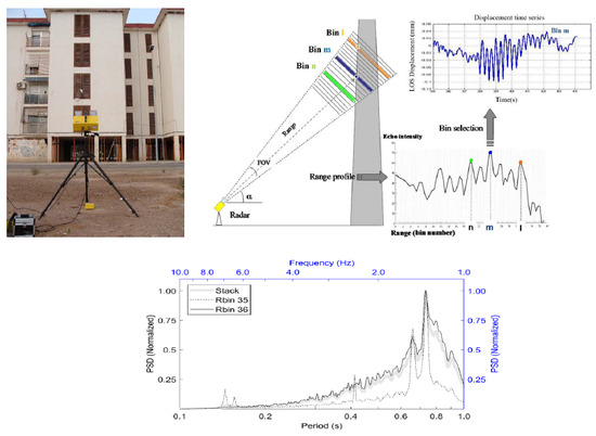
2.1. The RAR Basics and Survey

The use of interferometric radar to evaluate the vibration state of structures as bridges, has been investigated since the nineties [13] and RAR based methods became consolidated in the following decade [14,15,16], so that nowadays commercial systems [17] are available. Several papers have been published about the monitoring of bridges [18,19,20], wind turbine towers, [21], buildings [22,23], and towers [24,25,26]. In the last years also the development of novel systems has been suggested by different research groups [27,28,29].
According to the meaning of its acronym RADAR, Radio Detection And Ranging, a radar device is able to detect and range objects. The radar acquires echoes from the different targets contained in its antenna Field Of View (FOV). The amplitude peaks detected at different times correspond to contributions from parts of the observed structure located at different distances. According to the radar equation, the operating distance and the characteristics of the backscattering surface strongly affect the radar response. A radar observation uses the time elapsed between the transmission and reception of an electromagnetic waveform to provide a signal, usually called range profile, composed by peaks of different amplitudes, which identify the main reflecting parts of the observed structure. Points of the range profile are usually called radar bins (Rbin) and they correspond to sampling volumes around targets located at different distances from the radar. The intersection between these elemental solid angle units and the surface of the monitored structure, in which the transmitted waves are backscattered, determines the capability to sample unambiguously the monitored structure, with separated elements. The measurement procedure consists of three main steps. First, the amplitude profile as a function of the range, sampled at regular spatial steps, is collected. Afterwards, when the intensity of the radar echo coming from these elements assures an adequate Signal-to-Noise Ratio (SNR), the corresponding part of the structure can be associated to the interferometric phase of the echo; third and last, a displacement time history is derived by the time variations of the phase, by using the following equation:
d L O S t = λ 4 π Δ φ t
where Δ φ t is the difference between the phases measured in two successive radar acquisitions and λ is the wavelength of the transmitted wave. The retrieval of the Line Of Sight (LOS) displacement from the measured differential phase of the received radar signal, with sub-millimetric accuracy, is possible because coherent radar provides also the phase value of the reflected signal, which allows, through interferometry, for the evaluation of range variations in terms of fraction of wavelength of the propagating radar wave. When the displacement ranges within ±λ/4, the phase change is linearly related to the variation of the distance occurred between two successive radar acquisitions as stated by equation (1). Considering that, in our case, λ/4 is larger than 4 mm and that the expected structure displacements range from millimeters to tens of microns, this linear hypothesis does work. Moreover, according to equation (1), the shorter the wavelength, the higher the sensitivity of the measurement in terms of displacement. For a radar operating in the Ku band with a wavelength of λ = 1.76 cm (operating frequency = 17 GHz), a phase variation of 1°, typically achievable using a state-of-the-art sensor, corresponds to a displacement of approximately 20 microns: the expected displacement accuracy, at best measuring conditions (high SNR), is of the order of tens of microns. On of the main limitations of this technique is that considering more generally a three-dimensional displacement, d t   the proposed technique can only estimate the projection of d t in the LOS direction. Therefore, when d t is perpendicular to the LOS, the displacement vector d t cannot be observed by the radar. Figure 1 shows a picture of the RAR device and a scheme of the basis of the RAR method explained above.
The Centre Tecnològic de Telecomunicacions de Catalunya (CTTC) owns a commercial radar device with interferometric capability: the IBIS-S manufactured and marketed by Ingegneria dei Sistemi SpA (IDS). The RAR device embodies a sensor module, a control PC, a power supply unit and also it includes data processing software (see Figure 1a). The sensor module transmits an electromagnetic signal at a central frequency of 17.2 GHz (Ku band) with a maximum bandwidth of 300 MHz, corresponding to a range resolution of 0.5 m. Range resolution is herein understood as the minimum distance between two targets necessary to be separated, that is, seen as two different subsequent bins. The radar instrument is mounted on a tripod, which is equipped with a rotating head to adjust the bearing of the sensor towards the surveyed structure. The main characteristics of this sensor are summarized in Table 1.
The maximum acquisition rate is 200 Hz. Details on the radar equipment can be found in [23]. The antennas used in this work are two pyramidal horns with a high gain (Gain = 23.5 dB) to improve the SNR of the radar measurement. The bins corresponding to the best SNR are usually selected. The sensor unit is managed by a PC-based control unit, through a standard USB communication, which is provided with software used to configure the acquisition parameters, store the measurement data, and show the displacements in real time. The power supply unit provides about 5 hours of autonomy. The main characteristic of this device and its incorporated microwave technology is the capability of a straightforward measurement of displacements with amplitudes down to tens of microns. In addition, an advantage of the equipment is its ease of use and portability in almost any schedule and weather condition.

2.2. Data Acquisition

The RAR device described above was used to monitor the displacement time history of the vibration of the surveyed building. On September 14, 2012 the RAR system was installed in the San Fernando neighborhood of the city of Lorca. The Radar location, distance to the building and observation angle were selected for the highest SNR and providing a detectable LOS component of the building displacement with respect to the accuracy of the system. The Radar was located 17.1 m far from the facade and with an average elevation angle with respect to the horizon of 37° (α in Figure 1b). Recall that RAR device measures dLOS, that is, the displacement along the LOS. In addition, it is worth noting that the RAR device identifies the different parts of the building with an accuracy of approximately 0.5 m in height. In general, it is expected that bins with higher SNR would provide better accuracy in measuring the differential phase, but another factor to take into account, in order to evaluate the detection capability of the technique, is the angle of incidence of the LOS with respect to the vibrating surface. For low incidence angles, displacements seen by the radar are closer to the actual horizontal displacement while increasing the angle the fraction measured of horizontal displacement decreases. Otherwise, it is also true that higher points would exhibit larger horizontal displacements. The radar and building positions are shown in Figure 2a1,a2. Therefore, a crucial issue in RAR-based analysis is to identify and to choose the bins best representing the vibration of the target building. This is not an easy task, which is not free from several doses of expert judgment. To help in this important issue, RAR device provides two sources of information: (i) a Signal-to-Noise (SNR) profile and (ii) an accuracy profile. Figure 2b,c, shows these two profiles in our case. Bins that correspond to the highest SNR peaks and highest accuracy (lowest values in the accuracy profile) are usually good candidates to analyze their displacement time series and to estimate the vibrating frequency of the monitored structure.
Thus, according to these two profiles, Rbins numbers 35, 36, 41, 42, and 43 could be eligible. However, an analysis in the frequency domain of these time histories shows that clear vibrating periods in the 0.1–1.0s range of periods, are clearly seen only in Rbins numbers 35 and 36 (see Figure 2). Moreover, noticeably, the accuracy profile is obtained using the so called effective SNR (eSNR), which is different from the SNR profile shown in Figure 2b and takes into account the contribution of radar clutter; that is, the influence of vibrating objects included in the same bin, which can worsen the interferometric measurement [17]. Probably this is the main cause of the bad quality of the Rbins from 41 to 43. Thus, time histories of Rbins 35 and 36 have been chosen for the analysis. Note that for these two Rbins good enough SNR and high accuracy are obtained (see Figure 2).

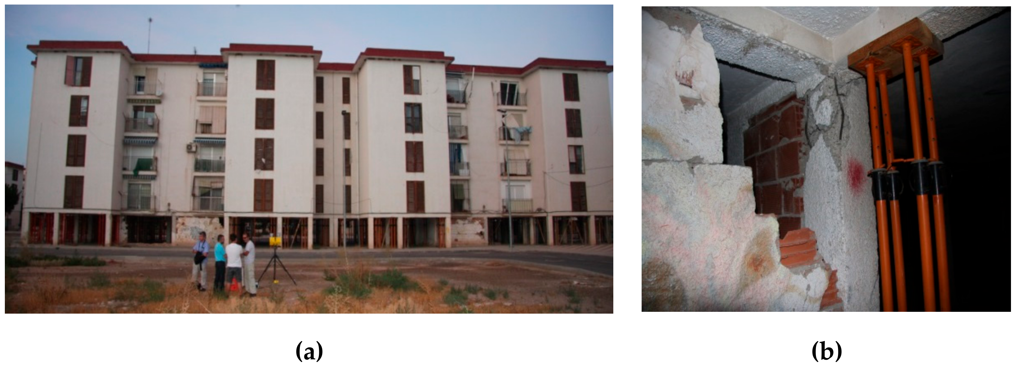
2.3. The Building. Structural Description and Numerical Model

The RAR-surveyed building was carefully modeled. This building was one of fifteen residential buildings located in the San Fernando neighborhood in Lorca (see Figure 3a). The design for most of the buildings in the neighbourhood was based on an open-plan space in the ground level in order to face severe floods as those occurred in the region during the 1960–70 decade. This soft-story configuration clearly influenced the building seismic performance because of the concentration of shear forces and displacements on the weaker frames, induced by abrupt changes of stiffness in height [30,31,32]. This effect was commonly referred to as the failure mechanism in the damage report completed by experts after the earthquake [33]. Moreover, the described damage distribution mainly affected this first level. The few infill walls in the entrance (first level) of most buildings collapsed, and the typical infill failure was described as induced by the movement of the surrounding frame. Regarding the pillars of the first level, shear damage appeared at the bottom and top ends of almost all pillars. Figure 3b shows a detail of a damaged pillar. Minor damages were observed in the upper levels [33]. Noticeably, buildings in this neighborhood were demolished and they were substituted by new constructions.
The damaged building was a reinforced-concrete-moment-frame structure with unidirectional slabs having a thickness of 20 cm and closed with infill-unreinforced brick-masonry walls. The building had five stories and six spans in the studied direction.
Figure 4 shows the floor plan and a sketch of the cross section of a module. Foundations were conceived by pile caps with ground beams. Cross-sections of the pillars, in all cases, are squared and their dimensions and reinforcing steel vary in a few pillars in the first two levels, remaining homogeneous in the upper levels. The longitudinal and transverse reinforcing steel of the frames is very poor and does not meet the reinforcing requirements foreseen in current seismic codes. Table 2 shows the details of sections and reinforcing steel for pillars and beams. All these issues confirm that the building was designed without any consideration of the somehow moderate but significant seismic hazard in the region. The compressive strength of the concrete equal to f′c = 2.06 kN/cm2 was taken from the original blueprints. According to the contemporary code, the reinforcing steel used at that time was the AE 42N with tensile strength fy = 41.18 kN/cm2. Loads were applied according to the recommendations of Eurocode 8 [34].
The building was modeled and analyzed by using the SAP2000 software [35]. Beams and pillars were modeled by using frame type elements. In order to consider their yielding surfaces, P-M2-M3 hinges, with a flexural–shear interaction, were located at both ends of each element in pillars and M3 hinges at both ends of principal and secondary beams according to the ASCE 41-13 [36]. For details on P-M2-M3 and M3 hinges see the SAP 2000 software manual [35]. The slab was considered to behave as a semi-rigid diaphragm and it was modeled by means of an equivalent linear membrane element with homogeneous thickness. Infill walls were modeled with a single nonlinear membrane element for panels without openings. In the case of walls with openings and, according to failure modes found in literature, the panel was modeled with a linear membrane in the rigid zones, and with a nonlinear membrane in the zones where damage may appear. Geometric non-linearity was also considered by including the P-Delta effect.

3. Results

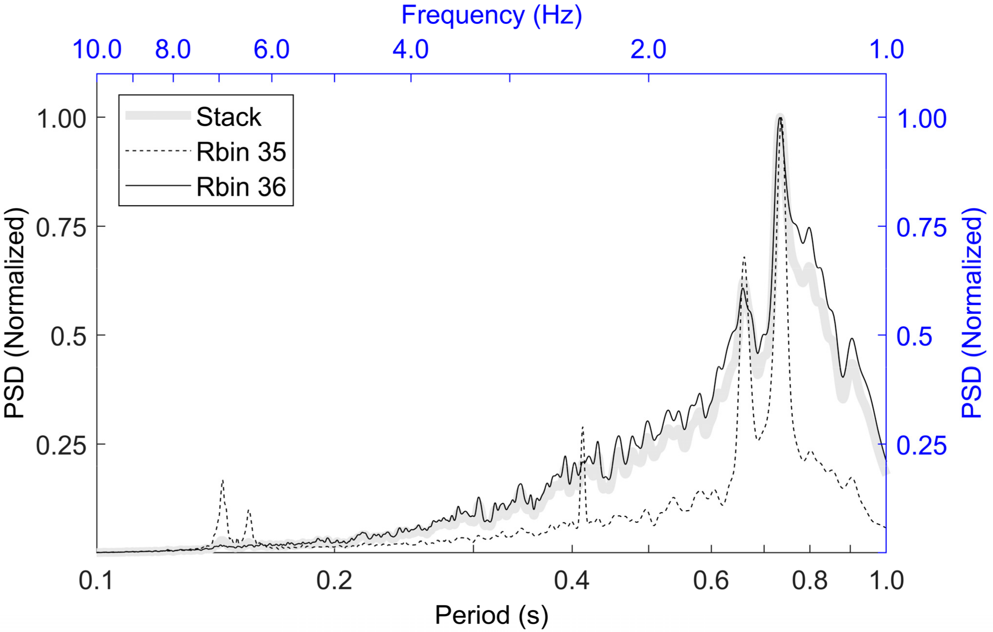
3.1. Data Analysis (RAR)

As a preliminary step, radar bins are analyzed in the time and frequency domains. Figure 5a shows the signals in the time domain. Raw data and filtered data are shown. A third order band-pass Butterworth causal filter was applied in the frequency band 0.1–10.0Hz. Figure 5b shows the analysis in the frequency domain. The Welch method [37,38], as implemented in Matlab software [39], was applied to compute the Power Spectral Density (PSD).
The raw data were collected at a sampling rate of 144 Hz and the duration of the signal was 35 minutes. For the Welch method, Hamming windows with 95% overlap were used and the length of the windows was 2.2 minutes, so that the resolution in the frequency domain was higher than 0.01 Hz (Δf = 0.0077Hz). For clarity, in Figure 5b, PSDs were normalized to the maximum value so that mean PSD values range between 0 and 1. Black lines are the mean values and red dashed lines correspond to 95% confidence upper and lower bounds. As pointed out above, no clear frequencies can be seen in the 0.1–1.0 period range with the only exception of Rbins 35 and 36. Rbins 41, 42, and 43, which also show good enough SNR and accuracy in Figure 2, probably are contaminated by other vibrating objects hiding the actual structural vibration. Thus, only Rbins 35 and 36 are used in the following analysis. Figure 6 shows the raw and filtered displacement time series in the time and frequency domains. In this case, the band-pass of the filter is 1.25–10.0Hz. The corresponding PSD are also shown in the lowest subplots.
In order to improve the quality of the analysis, Rbins 35 and 36 were stacked in the time domain. It is well known that staking enhances coherent components and abates other incoherent components. The stacking technique is commonly used in seismology. Stacking seismic data is oriented to enhance coherent signals and soften random signals, that is, noise. The SNR of the output trace should be higher than that of a single trace. Figure 7 shows the normalized PSDs of Rbins 35, 36 and the one of the stacked signals. Clear peaks are found at periods of 0.66 s and 0.73 s (frequencies of 1.51 Hz and 1.36 Hz). Other peaks, for example those included in the interval 0.1–0.2 s. and present only in Rbin 35, are smoothed when Rbin 35 and Rbin 36 are stacked. These two peaks are assumed to correspond to the structural free vibration of the building.

3.2. Building Modal Analysis and Capacity Curve

A modal analysis was performed on the numerical model of the undamaged building generated with the SAP2000 software [35]. The obtained results are shown in Table 3.
It can be seen how periods of the three main modes of vibration are within the expected range of periods when buildings with similar characteristics are considered, that is, in the range from 0.08 n to 0.13 n seconds, where n is the number of levels [40]. In Figure 4, the X- and Y-axes are respectively the long (longitudinal) and short (transversal) directions.
The capacity curve and the corresponding capacity spectrum, in the Y direction, were then obtained by means of the well-known pushover analysis (see for instance FEMA-440 [41]). Figure 8 shows the capacity curve and capacity spectrum, together with their bilinear curves [41].
Table 4 displays the characteristic points of these two curves. That is, the yielding and ultimate capacity points and the maximum values of the shear forces, in the capacity curve, and the corresponding maximum values of the spectral acceleration, Sa, in the capacity spectrum.

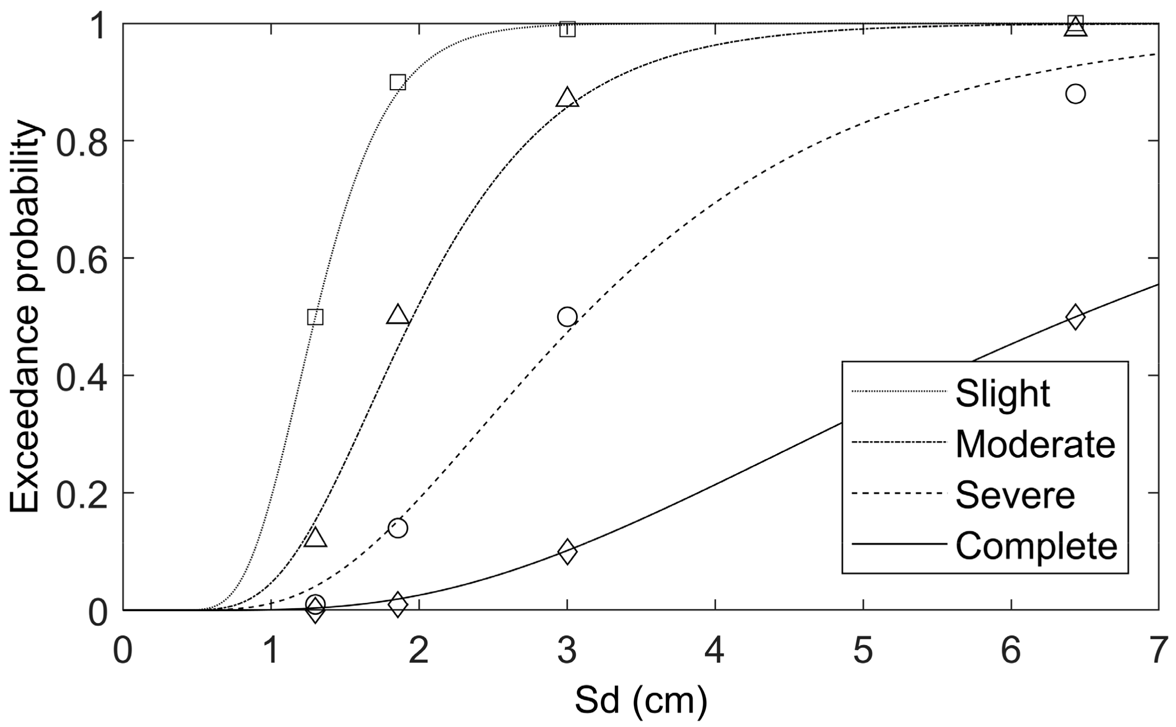
3.3. Expected Performance, Fragility, and Damage

In this section the performance and expected damage of the building subjected to the seismic actions of the Lorca 2011 earthquake are analyzed.
Figure 9 shows the two horizontal accelerograms recorded at a station located about 1.5 km from the site of the studied building. A sketch of the locations of the epicenter, accelerometer and building is also shown in this figure. Accelerograms are shown in the time and frequency domains, Fourier amplitude spectrum (FAS). In addition, response spectra, in the T-Sa and Sd-Sa formats are also depicted. The periods of the building (see Table 3) have been highlighted. Peak ground accelerations are 360 and 152 cm/s2, for the N30W and E30N components, respectively. The N30W accelerogram has been used as a likely seismic action, which affected the building.
The performance point defines the roof-displacement that the seismic action produces in the building and it represents the maximum expected displacement of a control node in the roof of the building. The performance point has been obtained following the procedure A, described in FEMA-440 [41].
This performance point (Sd = 3.2 cm, Sa = 0.23 g) is also shown in Figure 8 above. The period corresponding to this point is 0.75 s.
For a given damage state, the corresponding fragility curve defines the probability of reaching or exceeding this damage state as a function of a parameter representative of the severity of the seismic action [42]. This parameter, in our case, is the spectral displacement, Sd. Usually, fragility curves are described by lognormal cumulative functions and, this way, they are fully defined by means of the mean value, μ, and the standard deviation, β, of the lognormal function. In the framework of the European project Risk-UE, a simplified procedure, allowing setting up fragility curves starting from the bilinear form of the capacity spectrum, was proposed [43,44]. Four non-null damage states are considered. Namely 1. Slight, 2. Moderate, 3. Severe and 4. Complete. Mean values are determined by means of the following equation:
μ 1 = 0.7 S d y ;   μ 2 = S d y ;   μ 3 = S d y + 0.25 S d u S d y ;   μ 4 = S d u
are also called damage state thresholds. Standard deviations, βi, are then determined, from the following assumptions: (i) the exceedance probabilities of the damage state j, at the damage state thresholds are 50% and (ii) the probabilities of the other damage states follow a binomial distribution. A least squares fit leads to obtain the βj values. Figure 10 shows the obtained fragility curves. Points constructed according to conditions (i) and (ii), above, are also depicted in this figure. This procedure has been used in many seismic risk studies for European earthquake prone cities [45,46,47]. The damage state thresholds of equation (2) are based on expert opinion while the assumption ii) is based on damage observed in earthquakes [48].
For a given spectral displacement, Sd, and a given damage state dsi, fragility curves define the exceedance probabilities, P[d ≥ dsi |Sd], that damage, d, be equal or greater than the damage state, i, and, therefore, the probabilities of occurrence of each damage state, i, can be known by means of the following equation:
P 0 S d = 1 P d d s 1 | S d P i S d = P d d s i | S d P d d s i + 1 | S d           i 1 , 2 , 3 P 4 S d = P d d s 4 | S d  
Moreover, the mean damage state, MDS, as defined in Equation (4), is useful to represent the expected damage by means of only one parameter.
M D S S d = i = 0 4 i · P i S d
The index i = 0 corresponds to the Null or No-damage state. The indices i ∈ {1, 2, 3, 4} correspond respectively to Slight, Moderate, Severe and Complete damage states. Notably, MDS(Sd) in Equation (4) takes values between 0 and 4. MDS(Sd) = 0 means that the probability of the no-damage state is 1 and MDS(Sd) = 4 means that the probability of Complete damage state is 1. Figure 11 shows the mean damage state curve corresponding to the fragility curves of Figure 10. The spectral displacement of the performance point, Sd = 3.2 cm, is also plotted in Figure 11; the corresponding mean damage grade is 2.54 and the probabilities of the damage states 0. Null, 1. Slight, 2. Moderate, 3. Severe and 4. Complete, are 0.11, 0.36, 0.41, and 0.12, respectively. This damage distribution is also depicted in Figure 11. It means that 77% of this kind of buildings exposed to the seismic action of the Lorca 2011 earthquake would suffer moderate or severe damage and 12% would be close to collapse.
The damage observed in the building clearly suggested a first floor soft-story effect as an important contributor to damage. Thus, this effect has been analyzed by means of the study of the inter-story drifts. Figure 12 shows the displacements (Figure 12a) and inter-story drift ratios (Figure 12b) at the performance point (blue line) and at the ultimate capacity point (black line). Table 5 summarizes the obtained inter-story displacements and drifts ratios.
At the performance point, the maximum displacement (about 38% of the total displacement) is obtained in the first floor and the contribution to the total displacement decreases at higher floors.
The minimum displacement (about a 7% of the total displacement) is obtained in the uppermost floor. A drift ratio near 0.5% is obtained at the first floor. At the ultimate capacity point, the first floor displacement is about the 71% of the total displacement while the corresponding drift ratio is about 1.9%.
Displacements and drift ratios in the upper floors are similar to or lower than the ones corresponding to the performance point. These displacements and drift ratios clearly confirm the soft-story effect as the responsible for the observed damage.

4. Discussion

In this study, the feasibility of using natural vibrations to detect the safe/unsafe state of buildings has been investigated. Recent and promising works about monitoring buildings after earthquakes by means of remote sensing have been published [49,50]. In this work, remote sensing was performed by using a RAR device because the interferometric technology is capable of managing high frequency dynamic measurements with high resolution. This is an advantage of the RAR if compared with other tools such as LiDAR, InSAR, SAR imagery, aerial video footage, oblique imagery, point clouds from overlapping images, and aerial photography among other techniques. The starting hypothesis is that the modal properties of the building change with increasing damage. An easy to observe property is the fundamental period of the building that would increase with damage [12]. Thus, as a test bed, a building that was severely damaged by the Lorca, 2011, earthquake was surveyed with a RAR device. Unfortunately, additional measures inside the building could not be taken because access inside the building was prohibited by local authorities due to safety reasons. For sure, it would be preferable to combine the displacement time histories obtained with the RAR device with acceleration and/or velocity time histories taken in different floors and positions inside the building as it was done in the building surveyed in reference [23]. Moreover, it should be taken into account that we are dealing with extremely low amplitudes. The root mean square (RMS) amplitude of the filtered Rbin35 is 0.004 mm (4 μm) and the one of Rbin 36 is 0.025 mm (25 μm); thus, special care has to be taken when dealing with this kind of really weak signals. However, the high performance of last generation RAR devices together with high resolution of interferometric techniques and signal analysis methods allowed us to obtain good enough results. Two clear periods are identified: 0.77 s and 0.66 s, which are assumed to be linked to the periods of the undamaged structure, of the first mode, in the Y direction, 0.570 s, and to the rotational one around Z axis, 0.567 s. (see Table 3). The fact that periods obtained from RAR measurements are longer is attributed to damage. However, in this kind of study, an important question is how to know the vibrations properties of the undamaged/safe building and how the period evolves with damage. There were no undamaged buildings of this typology after the earthquake. Therefore, an important effort was focused on the numerical modeling of the building. In spite that the mechanical and geometrical properties of the building were well known, because accurate technical post-earthquake reports were available [33], the strength parameters of the mechanical model were also calibrated. This was done in such a way that the expected period of vibration of the building at the performance point matched well the one obtained from the RAR measurements; a period of 0.75 s, which is very close to the longest period found in the RAR displacement time histories. Moreover, capacity spectrum-based methods [43,44,45,46,47] allowed obtaining fragility curves, mean damage states and damage probability matrices. The mean damage state at the performance point is 2.54, which corresponds to probabilities of Severe and Complete damage states of 41% and 12% respectively. Remarkably this damage distribution is also in agreement with the damage observed and reported after the Lorca 2011 earthquake [51].

5. Conclusions

The main conclusions of this work are as follows. Concerning the interferometric RAR-based devices and methods, they may become excellent tools allowing for fast and easy measurements of the fundamental vibration features of actual buildings. In the present study, the remote sensing data usefully collected are only two range-bins time series from a single acquisition station. This means that the modal parameters cannot be fully reconstructed. Nevertheless, in the context of the surveyed building, the fundamental vibration modes were detected. These tools and methods may be especially useful in post-earthquake surveys of severely damaged buildings because, when adequately calibrated, the obtained results allow for estimating the damage state of the building from remote sensing measurements that do not require entering damaged buildings, thus avoiding risky check-ups inside severely damaged buildings that could collapse during the inspection works. However, it is also true that, for the success of damage diagnosis, it is very important to know the initial conditions of the undamaged building.
Concerning the surveyed building, a detailed study based on blueprints and on details of the original construction revealed insufficient reinforcing steel in stirrups and in longitudinal reinforcements in pillars. Moreover, the analysis of the inter-story drifts pointed towards the soft story behavior of the first floor as the main source of damage. This effect was increased because of the abrupt change in the stiffness due to the absence of inner walls in the first floor. Therefore, it is straightforwardly concluded that the assessed building was designed without any consideration of the seismic hazard in the region and was built by following construction rules leading to poor reinforcement in concrete elements and to a weak seismic performance. These facts highlight the importance of seismic regulations, even in low-to-moderate seismic hazard regions.
The recent and growing interest in smart cities open up, ideally, to fascinating and widespread applications of this technique [52]. Buildings and structures, starting from those with higher strategic, social, cultural, and economic value, could be instrumented, so that their vibration characteristics could be monitored in a real-time basis. This way, any change in their modal properties could be detected and the cause of such modifications could be investigated. In fact, the cost of accelerometers and other devices allowing one to measure vibrations of buildings subjected to ambient noise is decreasing and the added cost of implementing such instruments and methods in new buildings and structures could be insignificant in comparison to the overall cost of the building. Ongoing and future research on this issue may lead to simplified procedures allowing for damage detection and, if the sensors distribution is adequate, it should be even possible to develop algorithms with the capability of detecting where and when the damage has been produced. In this respect, a final consideration of this research would be the recommendation to authorities, administrations and civil protection services to encourage the design and implementation of a building technical file which should include, among other parameters, the modal behavior of new structures, which could be measured at the end of their construction. This information should be crucial for damage assessment after extreme events, obviously including earthquakes, but also other hazardous or disastrous happenings.

Author Contributions

L.G.P., R.G.-D. and G.L. conceived, designed and managed this research. R.G.-D., L.G.P. and G.L. made the research of building information. G.L., L.G.P. and R.G.-D. acquired the RAR data. L.G.P. and G.L. wrote the computer codes to process the RAR data. E.C., Y.F.V.-A. and J.A.-H. analysed the building floor plans and obtained the numerical model of the building. L.G.P., E.C., Y.F.V.-A. and R.G.-D. wrote the computer codes to obtain the capacity, fragility and the performance of the building and the evaluation of the damage. R.G.-D., E.C., L.G.P., and G.L. wrote the paper.

Funding

This research has been partially funded by the Ministry of Economy and Competitiveness (MINECO) of the Spanish Government and by the European Regional Development Fund (ERDF) of the European Union (EU) through projects with references CGL2015-65913-P (MINECO/ERDF, EU) and EFA158/16/POCRISC (INTERREG/POCTEFA. EU). Yeudy F. Vargas-Alzate has been granted an Individual Fellowship (IF) in the research grants program of the Marie Sklodowska-Curie Actions (MSCA) of the European Union/European (H2020-MSCA-IF-2017) No 799553. Esteban Cabrera, sponsored by the University of Azuay (UDA), obtained a scholarship from the Ministry of Higher Education, Science and Technology, SENESCYT, Government of Ecuador, for doctoral studies in the Earthquake Engineering program at UPC-Barcelona-Tech.

Acknowledgments

The authors are grateful to the Editors of the Remote Sensing Special Issue “Close Range Remote Sensing” for inviting them to submit this paper.

Conflicts of Interest

The authors declare no conflict of interest.

References

  1. Alarcón, E.; Benito, M.B. Foreword special issue Lorca’s earthquake. Bull. Earthq. Eng. 2014, 12, 1827–1829. [Google Scholar] [CrossRef]
  2. Vargas-Alzate, Y.F.; Pujades, L.G.; Barbat, A.H.; Hurtado, E.; Diaz, S.A.; Hidalgo-Leiva, D.A. Probabilistic seismic damage assessment of reinforced concrete buildings considering directionality effects. Struct. Infrastruct. Eng. 2018, 14, 817–829. [Google Scholar] [CrossRef]
  3. Pinzón, L.A.; Díaz-Alvarado, S.A.; Pujades, L.G.; Alva, R.E. Do Directionality Effects Influence the Expected Damage? A Case Study of the 2017 Central Mexico Earthquake. Bull. Seismol. Soc. Am. 2018, 108, 2543–2555. [Google Scholar] [CrossRef]
  4. Doebling, S.W.; Farrar, C.R.; Prime, M.B.; Shevitz, D.W. Damage Identification and Health Monitoring of Structural and Mechanical Systems from Changes in their Vibration Characteristics: A Literature Review; Los Alamos National Laboratory Report LA-13070-MS; USDOE: Washington, DC, USA, 1996. [Google Scholar]
  5. Sohn, H.; Farrar, C.R.; Hemez, F.M.; Czarnecki, J.J. A Review of Structural Health Monitoring Literature: 1996–2001; Los Alamos National Laboratory Report LA-UR-02-2095; USDOE: Washington, DC, USA, 2002. [Google Scholar]
  6. Farrar, C.R.; Worden, K. An introduction to structural health monitoring. Phil. Trans. R. Soc. 2007, 365, 303–315. [Google Scholar] [CrossRef] [PubMed]
  7. Farrar, C.R.; Lieven, N.A.J. Damage prognosis: The future of structural health monitoring. Phil. Trans. R. Soc. 2007, 365, 623–632. [Google Scholar] [CrossRef] [PubMed]
  8. Masciotta, M.G.; Roque, J.; Ramos, L.; Lourenço, P. A multidisciplinary approach to assess the health state of heritage structures: The case study of the Church of Monastery of Jeronimos in Lisbon. Constr. Build. Mater. 2016, 116, 169–187. [Google Scholar] [CrossRef]
  9. Capozzoli, L.; Rizzo, E. Combined NDT techniques in civil engineering applications: Laboratory and real test. Constr. Build. Mater. 2017, 154, 1139–1150. [Google Scholar] [CrossRef]
  10. Farrar, C.R.; Doebling, S.W.; Nix, D.A. Vibration-based structural damage identification. Phil. Trans. R. Soc. 2001, 359, 131–149. [Google Scholar] [CrossRef]
  11. Vidal, F.; Navarro, M.; Aranda, C.; Enomoto, T. Changes in dynamic characteristics of Lorca RC buildings from pre- and post-earthquake ambient vibration data. Bull. Earthq. Eng. 2014, 12, 2095–2110. [Google Scholar] [CrossRef]
  12. Farrar, C.; Darling, T.W.; Migliorini, A.; Baker, W.E. Microwave interferometer for non-contact vibration measurements on large structures. Mech. Syst. Signal Process. 1999, 13, 241–253. [Google Scholar] [CrossRef]
  13. Bartoli, G.; Facchini, L.; Pieraccini, M.; Fratini, M.; Atzeni, C. Experimental utilization of interferometric radar techniques for structural monitoring. Struct. Control Health Monit. 2008, 15, 283–298. [Google Scholar] [CrossRef]
  14. Pieraccini, M.; Luzi, G.; Mecatti, D.; Noferini, L.; Atzeni, C. A microwave radar technique for dynamic testing of large structure. IEEE Trans. Microw. Theory Tech. 2003, 51, 1603–1609. [Google Scholar] [CrossRef]
  15. Pieraccini, M.; Fratini, M.; Parrini, F.; Pinelli, G.; Atzeni, C. Dynamic Survey of Architectural Heritage by High-Speed Microwave Interferometry. IEEE Geosci. Remote Sens. Lett. 2005, 2, 28–30. [Google Scholar] [CrossRef]
  16. Gentile, C.; Bernardini, G. An interferometric radar for non-contact measurement of deflections on civil engineering structures: Laboratory and full-scale tests. Struct. Infrastruct. Eng. 2010, 6, 521–534. [Google Scholar] [CrossRef]
  17. Coppi, F.; Gentile, C.; Ricci, P.A. Software tool for processing the displacement time series extracted from raw radar data. In Proceedings of the 9th International Conference on Vibration Measurements by Laser and Non-Contact Techniques, Ancona, Italy, 22–25 June 2010. [Google Scholar]
  18. Pieraccini, M.; Fratini, M.; Parrini, F.; Atzeni, C. Dynamic monitoring of bridges using a high-speed coherent radar. IEEE Trans. Geosci. Remote Sens. 2006, 44, 3284–3288. [Google Scholar] [CrossRef]
  19. Gentile, C.; Bernardini, G. Output-only modal identification of a reinforced concrete bridge from radar-based measurements. NDT&E Int. 2008, 41, 544–553. [Google Scholar]
  20. Stabile, T.A.; Perrone, A.; Gallipoli, M.R.; Ditommaso, R.; Ponzo, F.C. Dynamic Survey of the Musmeci Bridge by Joint Application of Ground-Based Microwave Radar Interferometry and Ambient Noise Standard Spectral Ratio Techniques. IEEE Geosci. Remote Sens. Lett. 2013, 10, 870–874. [Google Scholar] [CrossRef]
  21. Pieraccini, M.; Fratini, M.; Parrini, F.; Atzeni, C.; Spinelli, P. In-service testing of wind turbine towers using a microwave sensor. Renew. Energy 2008, 33, 13–21. [Google Scholar] [CrossRef]
  22. Luzi, G.; Monserrat, O.; Crosetto, M. The Potential of Coherent Radar to Support the Monitoring of the Health State of Buildings. Res. Non-Destr. Eval. 2012, 23, 125–145. [Google Scholar] [CrossRef]
  23. Negulescu, C.; Luzi, G.; Crosetto, M.; Raucoules, D.; Roullé, A.; Monfort, D.; Pujades, L.G.; Colas, B.; Dewez, T. Comparison of seismometer and radar measurements for the modal identification of civil engineering structures. Eng. Struct. 2013, 51, 10–22. [Google Scholar] [CrossRef]
  24. Luzi, G.; Crosetto, M.; Cuevas-González, M. A radar-based monitoring of the Collserola Tower (Barcelona). Mech. Syst. Signal Process. 2014, 49, 234–248. [Google Scholar] [CrossRef]
  25. Gentile, C.; Saisi, A. Dynamic measurement on historic masonry towers by microwave remote sensing. In Proceedings of the International Conference on Experimental Vibration Analysis for Civil Engineering Structures, Varenna, Italy, 3–5 October 2011; Gentile, C., Benedettini, F., Eds.; Starrylink Editrice: Brescia, Italy, 2011; Volume II, pp. 524–530, ISBN 978-88-96225-39-4. [Google Scholar]
  26. Atzeni, C.; Atzeni, C.; Bicci, A.; Dei, D.; Fratini, M.; Pieraccini, M. Remote survey of the leaning tower of Pisa by interferometric sensing. IEEE Geosci. Remote Sens. Lett. 2010, 7, 185–189. [Google Scholar] [CrossRef]
  27. Grazzini, G.; Pieraccini, M.; Dei, D.; Atzeni, C. Simple Microwave sensor for remote detection of structural vibration. Electron. Lett. 2009, 45, 567–569. [Google Scholar] [CrossRef]
  28. Li, C.; Chen, W.; Liu, G.; Yan, R.; Xu, H.; Qi, Y. A Noncontact FMCW Radar Sensor for Displacement Measurement in Structural Health Monitoring. Sensors 2015, 15, 7412–7433. [Google Scholar] [CrossRef] [PubMed]
  29. Nair, A.; Cai, C. Acoustic emission monitoring of bridges: Review and case studies. Eng. Struct. 2010, 32, 1704–1714. [Google Scholar] [CrossRef]
  30. Kirac, N.; Dogan, M.; Ozbasaran, H. Failure of weak-storey during earthquakes. Eng. Fail. Anal. 2011, 18, 572–581. [Google Scholar] [CrossRef]
  31. Khan, D.; Rawat, A. Nonlinear Seismic Analysis of Masonry Infill RC Buildings with Eccentric Bracings at Soft Storey Level. Procedia Eng. 2016, 161, 9–17. [Google Scholar] [CrossRef]
  32. Benavent-Climent, A.; Mota-Páez, S. Earthquake retrofitting of R/C frames with soft first story using hysteretic dampers: Energy-based design method and evaluation. Eng. Struct. 2017, 137, 19–32. [Google Scholar] [CrossRef]
  33. Artés-Carril, J.M. Informe sobre actuaciones realizadas y daños en el grupo de 232 viviendas sociales del barrio de San Fernando de Lorca (Murcia) como consecuencia del terremoto del día 11-05-2011; Instituto de vivienda y suelo. Consejería de obras públicas y ordenación del territorio: Cantabria, Spain, 2011. (In Spanish) [Google Scholar]
  34. EC8, EN 1998-1. Eurocode 8: Design of Structures for Earthquake Resistance-Part 1. General Rules, Seismic Actions and Rules for Buildings, English Version; EN 1998-1:2004: E; European Committee for Standardization CEN: Brussels, Belgium, 2004. [Google Scholar]
  35. CSI. In CSI Analysis Reference Manual for SAP2000, ETABS and SAFE; Computer and Structures Inc.: Berkeley, CA, USA, 2016.
  36. ASCE, American Society of Civil Engineers. Seismic Evaluation and Retrofit of Existing Buildings; ASCE Standard ASCE/SEI 41-13; ASCE: Reston, VA, USA, 2014; ISBN 978-0-7844-1285-5. [Google Scholar]
  37. Welch, P.D. The use of Fast Fourier Transform for the estimation of power spectra: A method based on time averaging over short, modified periodograms. IEEE Trans. Audio Electroacoust. 1967, 15, 70–73. [Google Scholar] [CrossRef]
  38. Proakis, J.G.; Manolakis, D.G. Digital Signal Processing; Prentice-Hall: Upper Saddle River, NJ, USA, 1996; pp. 910–913. [Google Scholar]
  39. Matlab. Matlab the Language of Scientific Computing. The Mathworks Inc. 1994–2017. Available online: https://www.mathworks.com/ (accessed on 6 December 2018).
  40. NCSE-02, Norma de Construcción Sismorresistente. Parte general y Edificación; Spanish seismic Code; The Spanish Ministry of Development of the Spanish Government: Madrid, Spain, 2009. (In Spanish)
  41. FEMA-440. Improvement of Nonlinear Static Seismic Analysis Procedures; Applied Technology Council ATC-55 Project; FEMA-ATC: Redwood City, CA, USA, 2005.
  42. Vargas-Alzate, Y.F.; Pujades, L.G.; Barbat, A.H.; Hurtado, J.E. Capacity, fragility and damage in reinforced concrete buildings: A probabilistic approach. Bull. Earthq. Eng. 2013, 11, 2007–2032. [Google Scholar] [CrossRef]
  43. Milutinovic, Z.V.; Trendafiloski, G.S. RISK-UE Project of the EC: An Advanced Approach to Earthquake Risk Scenarios with Applications to Different European Towns; European Project EVK4-CT-2000-00014, European Commission. WP4 Vulnerability Curr. Build. 2003. [Google Scholar]
  44. Lagomarsino, S.; Giovinazzi, S. Macroseismic and mechanical models for the vulnerability and damage assessment of current buildings. Bull. Earthq. Eng. 2006, 4, 415–443. [Google Scholar] [CrossRef]
  45. Lantada, N.; Pujades, L.G.; Barbat, A.H. Vulnerability index and capacity spectrum based methods for urban seismic risk evaluation: A comparison. Nat. Hazards 2009, 51, 501–524. [Google Scholar] [CrossRef]
  46. Barbat, A.H.; Pujades, L.G.; Lantada, N. Seismic damage evaluation in urban areas using the capacity spectrum method: Application to Barcelona. Soil Dyn. Earthq. Eng. 2008, 28, 851–865. [Google Scholar] [CrossRef]
  47. Pujades, L.G.; Barbat, A.H.; Gonzalez-Drigo, R.; Avila-Haro, J.; Lagomarsino, S. Seismic performance of a block of buildings representative of the typical construction in the example district in Barcelona (Spain). Bull. Earthq. Eng. 2012, 10, 331–349. [Google Scholar] [CrossRef]
  48. Grünthal, G. European Macroseismic Scale; Centre Européen de Géodynamique et de Séismologie: Luxembourg, 1998; Volume 15. [Google Scholar]
  49. Contreras, D.; Blaschke, T.; Tiede, D.; Jilge, M. Monitoring recovery after earthquakes through the integration of remote sensing, GIS, and ground observations: The case of L’Aquila (Italy). Cartogr. Geogr. Inf. Sci. 2015. [Google Scholar] [CrossRef]
  50. Liu, W.; Yamazaki, F. Extraction of Collapsed Buildings in the 2016 Kumamoto Earthquake Using Multi-Temporal PALSAR-2 Data. J. Disaster Res. 2017, 12, 241–250. [Google Scholar] [CrossRef]
  51. Santamaría, G.P.; González López, S.; Alguacil, L. Analysis of consequences and Civil Protection activities in the Lorca earthquake Murcia): Pre-emergency, Emergency and Post emergency. Física de la Tierra 2012, 24, 343–362. (In Spanish). Available online: http://revistas.ucm.es/index.php/FITE/article/download/40144/38572 (accessed on 4 February 2019).
  52. Peris-Ortiz, M.; Bennett, D.G.; Pérez-Bustamante, Y.D. Sustainable Smart Cities: Creating Spaces for Technological, Social and Business Development; Springer: Berlin/Heidelberg, Germany, 2016; ISBN 9783319408958. [Google Scholar]
Figure 1. (a) The Real Aperture Radar (RAR) device; (b) Scheme of the basis of the RAR method. (See explanation in the text).
Remotesensing 11 02830 g001
Figure 2. (a1) RAR device and building; (a2) Plan view of the acquisition point; (b) Signal-to-noise-ratio (SNR); (c) accuracy plots of the RAR signals. Rbin 35 leads to the time series with the best quality data, due to high SNR (45 dB) and great accuracy (0.006 mm).
Remotesensing 11 02830 g002
Figure 3. (a) Typical buildings in San Fernando neighbourhood; (b) Example of a damaged pillar.
Remotesensing 11 02830 g003
Figure 4. Surveyed building: (a) Floor plan with the frame distribution. Arrows indicate the orientation of unidirectional slabs; (b) Cross-section of a module.
Remotesensing 11 02830 g004
Figure 5. (a) Rbins collected during the RAR survey. Raw and filtered data are shown; (b) Power Spectral Density (PSD) obtained by means of the Welch method. (See explanation in the text).
Remotesensing 11 02830 g005
Figure 6. Displacement time histories (a), Fourier spectra (b) and PSD (c) of Rbin35 and Rbin36.
Remotesensing 11 02830 g006
Figure 7. PSDs of Rbin35, Rbin36 and stacked signals. PSDs have been normalized to the maximum PSDs amplitudes. PSD are shown as functions of the frequency and the period.
Remotesensing 11 02830 g007
Figure 8. Capacity curve (left and below axes) and capacity spectrum (right and above axes) and their corresponding bilinear representations for the Y-direction.
Remotesensing 11 02830 g008
Figure 9. Horizontal accelerograms recorded at the Lorca accelerometric station. (a) N30W accelerogram; red circle corresponds to the peak ground acceleration, (b) E30N accelerogram. Red circle corresponds to peak ground acceleration. (c) Fourier amplitude spectra. (d) 5% damped response spectra. Red and pink circles correspond to the periods of the building (see Table 3). (e) 5% damped response spectra in Sd-Sa format; red circles and pink squares correspond to the periods of the building. The locations of the site, accelerometric station and epicenter are also sketched.
Remotesensing 11 02830 g009
Figure 10. Fragility curves for the modeled building in the +Y-direction. Square, triangle, circular and diamond markers correspond to the points determined by means of conditions (i) and (ii) above, which are used for the least squares fits.
Remotesensing 11 02830 g010
Figure 11. Mean damage state curve (a) and damage state probabilities in the performance point (b). The circle in (a) corresponds to the performance point.
Remotesensing 11 02830 g011
Figure 12. (a) Lateral displacements and (b) inter-story drift ratios at the performance point (blue line) and at the ultimate capacity point (black line).
Remotesensing 11 02830 g012
Table 1. Main operating parameters of the RAR device.
ParameterOperating FrequencyMax. Operational DistanceMax. Range ResolutionNominal Displacement AccuracyMax. Acquisition RateWeight/Battery Autonomy
Value17.2 GHz (Ku band)1000 m0.5 m10−5 m200 Hz12 kg/5 h
Table 2. Details of beams, sections, and reinforcing steel in the surveyed building.
SectionDimensions (cm)Reinforcing Steel
LongitudinalStirrups
Principal beams
Remotesensing 11 02830 i001
A = 254 ϕ 141 ϕ 6 / 18 cm
Secondary beams
Remotesensing 11 02830 i002
B = 25
c = 20
4 ϕ 141 ϕ 6 / 18 cm
Pillars
Remotesensing 11 02830 i003
d1 = 30 (*)4 ϕ 141 ϕ 6 / 15 cm
4 ϕ 141 ϕ 6 / 20 cm
4 ϕ 161 ϕ 6 / 22 cm
D = 254 ϕ 121 ϕ 6 / 15 cm
4 ϕ 141 ϕ 6 / 18 cm
4 ϕ 161 ϕ 6 / 18 cm
(*) Refers to several pillars on the first level.
Table 3. Results of the modal analysis.
ModePeriod (s)Mass Participation (%) Axis
10.57084.1Horizontal Y
20.56784Rotational Z
30.45473Horizontal X
Table 4. Main characteristics of the capacity curve and capacity spectrum for the Y-direction.
Capacity CurveCapacity Spectrum
δroof (cm)Base Shear (kN)Sd (cm)Sa (g)
Yielding point2.002256.21.820.20
Maximum shear force3.052319.02.810.24
Ultimate displacement6.761763.56.430.17
Table 5. Inter-story displacements and drifts corresponding to the performance point and to the ultimate capacity point.
Performance PointUltimate Capacity Point
StoryDispl. (cm)Drift Ratio (%)Contribution %Displ. (cm)Drift Ratio (%)Contribution %
11.210.46384.851.8771
20.770.29240.860.3213
30.560.21180.520.198
40.410.15130.350.135
50.230.0870.190.073

