MASS-UMAP: Fast and Accurate Analog Ensemble Search in Weather Radar Archives
by
 , , ,
, , ,
Gabriele Franch
1,2,* ,
,
Giuseppe Jurman
1 ,
,
Luca Coviello
1,
Marta Pendesini
3 and
Cesare Furlanello
1 1
Predictive Models for Biomedicine and Environment, Fondazione Bruno Kessler, 38123 Trento, Italy
2
Department of Information Engineering and Computer Science (DISI), University of Trento, 38123 Trento, Italy
3
Meteotrentino, 38122 Trento, Italy
*
Author to whom correspondence should be addressed.
Remote Sens. 2019, 11(24), 2922; https://0-doi-org.brum.beds.ac.uk/10.3390/rs11242922
Submission received: 30 September 2019
/
Revised: 23 November 2019
/
Accepted: 3 December 2019
/
Published: 6 December 2019
(This article belongs to the Special Issue Radar Meteorology)
Abstract
:The use of analog-similar weather patterns for weather forecasting and analysis is an established method in meteorology. The most challenging aspect of using this approach in the context of operational radar applications is to be able to perform a fast and accurate search for similar spatiotemporal precipitation patterns in a large archive of historical records. In this context, sequential pairwise search is too slow and computationally expensive. Here, we propose an architecture to significantly speed up spatiotemporal analog retrieval by combining nonlinear geometric dimensionality reduction (UMAP) with the fastest known Euclidean search algorithm for time series (MASS) to find radar analogs in constant time, independently of the desired temporal length to match and the number of extracted analogs. We show that UMAP, combined with a grid search protocol over relevant hyperparameters, can find analog sequences with lower mean square error (MSE) than principal component analysis (PCA). Moreover, we show that MASS is 20 times faster than brute force search on the UMAP embedding space. We test the architecture on real dataset and show that it enables precise and fast operational analog ensemble search through more than 2 years of radar archive in less than 3 seconds on a single workstation.
Keywords:
similarity search; precipitation; UMAP; MASS; PCA; dimensionality reduction; nowcasting; analog ensemble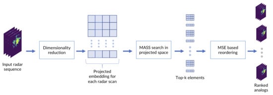
1. Introduction
The observation of repeating weather patterns has a long history [1], and the use of analogs has found its way in almost all aspect of meteorology, for the most diverse purposes. Approaches based on analogs have been proposed for the postprocessing of numerical weather predictions [2], as a statistical downscaling technique [3] and for data assimilation in numerical models [4,5]. However, the most prolific use of analogs is by far forecasting: either as a proxy for predictability [6], or as prediction technique itself [7]. In this regard, one of the most used operational methods for analog-based forecasting is Analog Ensemble (AnEn) [8], which involves searching and using an ensemble of past analogs to generate new deterministic or probabilistic [8] predictions. Ensemble methods have been used for very complex prediction targets, like short-term wind [9] or renewable energy forecasting [10]. Analogs can be sought to match single locations (pointwise time series) or spatial distributions over an area (spatio-temporal sequences). The quality of the analogs is totally dependent on the dimensionality of the data archive [11]: depending on the context, the historical records can spawn from few years to multiple decades, making the analog search procedure a critical component of any operational analog application method. The ideal analog search method should be dependable, predictable, accurate, fast, and able to return multiple ranked analogs at the same time. In this paper we present a novel search method for spatio-temporal sequences and show how it meets many of these desirable qualities.
In nowcasting applications (very short-term prediction, between 0 to 6 h), where the available time for computation is extremely limited, it is often necessary to trade-off analog search accuracy in favor of speed to meet a given computational time threshold. In this regard, one of the most important and complex problems is nowcasting precipitation fields. Analog ensemble approaches based on radar precipitation fields have been proposed for this application [12,13,14]: in particular, the AnEn method is especially relevant, as the nowcasting of convective precipitations is extremely challenging to tackle by Numerical Weather Prediction (NWP) methods [15]. AnEn approaches to radar nowcasting use feature extraction [12], linear dimensionality reduction [16], or cross-correlation [14] to summarize and perform an Euclidean search through the radar image archive, in combination with other indicators like mesoscale variables, seasonality, and time of the day to filter the pool of valid sequences.
In this work we propose a flexible framework that employs a two-step process that can be used to improve the accuracy and dramatically speedup the retrieval of spatiotemporal analog sequences. Our work combines nonlinear geometric dimensionality reduction method based on Uniform Manifold Approximation and Projection [17] (UMAP) with the fastest Euclidean-based profile search algorithm (Mueen’s Algorithm for Similarity Search [18] (MASS)), that can search for arbitrarily long time sequnces in constant time. We compare UMAP dimensionality reduction with principal component analysis (PCA) [19] on a original test dataset of almost 10 years of radar data, and show that UMAP finds analogs with smaller Mean Squared Error (MSE) than the one extracted by the PCA based method proposed in [16], with proper train configurations parameters. Moreover, we discuss how the MASS search algorithm is 20 times faster than linear Euclidean search and how it can be used to search the reduced UMAP space to find arbitrarily long time sequences of analogs in constant time. Finally, we discuss the flexibility of the UMAP-MASS method by showing how other indicators can be easily integrated in the search space to filter analogs and how it is feasible to fine-tune the dimensionality reduction using a custom distance function to project the embeddings.
2. Materials and Methods
2.1. UMAP: Uniform Manifold Approximation and Projection
Uniform Manifold Approximation and Projection [17] (UMAP) is a recent manifold learning technique for dimensionality reduction aiming at reconstructing in a lower dimensional space the geometric structure of the variety where data lie. UMAP is based on algebraic techniques mapping the original manifold into a reduced projection using topological analysis of the geometric space. UMAP is thus situated in the family of k-neighbour based graph learning algorithms (e.g., Laplacian Eigenmaps, Isomap, and t-SNE) and combines approximate k-nearest neighbor calculation (Nearest-Neighbor Descent) and a stochastic gradient descent for efficient optimization (SGD). Due to its faithfulness in the representation and the low computational burden, UMAP is becoming the reference algorithm for dimensionality reduction in multiple research fields [20]. The dimensionality reduction of UMAP is driven by four parameters: , number of components (d), number of neighbors (n), and minimum distance ( [21].
The parameter is the distance function used to compare elements in the space of the input data. By default, UMAP uses the Euclidean distance function, but any non-negative symmetric function can be a valid UMAP metric.
The number of components d represent the size of the projected space where the transformed data will lie: for example with every input element will be reduced to a vector of four values.
The n parameter controls the number of nearest neighbors used for each point to build the local distance function, taking into account the trade-off between highlighting the details rather than the global picture when rearranging the input data. Using higher values will force UMAP to look at larger neighborhoods to estimate the structure of the data, while using small values will give more weight to local structures present in the data.
The parameter forces a minimum distance between points in the output space. A smaller value will allow UMAP to pack similar elements closer to each other and describe finer topological structure, which can be useful for example for clustering applications, while higher values will preserve the broader structure more.
In Table 1, we report a summary of the main parameters used in this work.
2.2. MASS: Mueen’s Algorithm for Similarity Search
One of the most important subroutines in time series analysis is searching for similar patterns to a query string. Any new algorithm or method that can speed up this task can potentially open new disruptive applications in any system that deals with time series and historical records. Mueen’s Algorithm for Similarity Search (MASS) [18] is probably the most interesting solution in the domain of Euclidean-based searches in the last few years, where it has spawn new research directions [22,23,24,25,26]. Recently, its application as an analog search function for forecasting time series of renewable energy has been proposed [27]. The key idea in MASS is to perform the search in the frequency domain by computing the fast Fourier transform (FFT) on the time series, and replace the loop typically used in similarity matching algorithms with a convolution operation between the query vector and the search archive vector, thus making the search routine independent of the query length. This makes the algorithm free from the curse of dimensionality: matching a long query takes the same time than matching a short one. For this reason, the algorithm complexity depends only on the size of the search archive and its complexity is in the worst case. MASS also produces all the distances from the query to all sub-sequences of the archive, allowing to find all the most similar profile in one single pass. Notably, MASS is parameter-free and can be easily parallelized by splitting the data archive vector in chunks.
2.3. Meteotrentino Radar Dataset
The data used for this study was provided by Meteotrentino, the official Civil Protection Weather Forecasting Agency of the Province of Trento, Italy. The agency operates, in conjunction with the Civil Protection of the Province of Bolzano, a single polarization Doppler C-Band Radar located on Mt. Macaion (1866 m.a.s.l.), in a very complex orographic environment in the center of the Italian Alps (N46°29’18”, E11°12’38”). The radar produces a scan every 5 min, for a total of 288 scans per day, and covers an area of 240 km of diameter (27,225 sq km). The radar has been in operation since 2000, at the beginning with different operating modes and frequencies. The most important upgrade and calibration of the radar was performed in 2010 with the installation of the digital receiver. Given the complex orography of the region, the lower degrees of the radar scan suffer from beam blockage and backscattering caused by the nearby mountains. The polar volume is filtered and corrected from backscattering and attenuation using a doppler correction filter. All the main products in use by the civil protection are generated starting from the corrected polar volume.
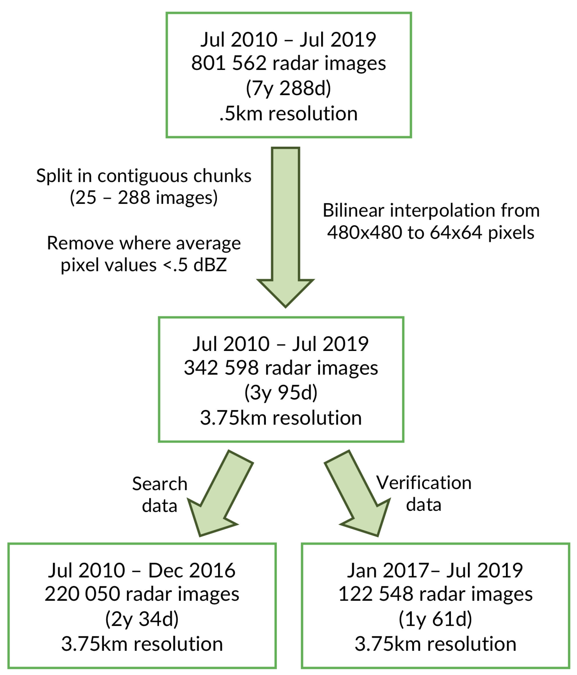
The product chosen for this study is the 2D MAX(Z) reflectivity (maximum on the vertical section) at 500 mt horizontal resolution that is currently in use by the civil protection for alerting and assessment purposes. The use of MAX(Z) is preferred over the more common constant altitude plain position indicators (CAPPI) because of the high operating altitude of the receiver, which would cause a constant altitude product to miss all precipitation events lower than the radar altitude. The range of recorded reflectivity values for the MAX(Z) product is 0 to 55 dBZ. Every scan is represented as a 480 × 480 floating point matrix over the bounding box coordinates: N47°12’39.9168”, S45°46’08.6412”, E12°19’45.3593”, W10°07’12.7347”. To guarantee a more homogenized product we considered the dates between July 2010 and July 2019, a time span where the radar setup and the quality of the product have been consistent. The total number of radar images in the period is , spanning seven years and 228 days, after accounting for missing data acquisition during the time period.
At least of the data in the archive consists of radar scans with no precipitation that its not interesting for the purpose of analog retrieval, so we removed most of it. This choice has also the effect of reducing the computation time of the analysis, and avoid data imbalance, even if UMAP is usually fairly robust against this issue. As the analog sequence retrieval process expects temporal continuity in the data, we developed a strategy to remove most of the empty data while keeping the temporal discontinuity of the resulting dataset to a usable level. Instead of working on single radar images, we divide the data in chunks of contiguous images by splitting the data by day. Due to missing scans we can obtain more than one chunk of contiguous data for the same day. Chunks longer than 2 h are kept, the rest is discarded, so each chunk contains at least 25 and at most 288 contiguous scans. Finally, we thresholded all chunks with no or few precipitation events: the sum of all pixel values of all images of each chunk is computed, and all chunks with an average pixel value dBZ are discarded. After these cleaning steps, the total number of samples in the dataset amounts to radar images, corresponding to three years and 95 days of precipitation data. For the reason stated above, and to avoid temporal overlapping, we split the dataset temporally between search space and verification: the data from the years 2010 to 2016 was used as archive (search space), and the years 2017–2019 as verification (query data). The final result is (two years and 34 days) images for search space and (one year and 61 days) for verification.
A simple bilinear resize was applied to all the selected data to obtain 64 × 64 pixel images, corresponding to a resolution of 3.75 × 3.75 km. This was chosen for similar reasons to the ones described in [16]: to reduce the computational time of the experiments and extend the range of tested parameters combinations; to remove small scale variability; and, in our case, to also remove any possible residual noise and scatter in the MAX(Z) product. Figure 1 summarizes the data preprocessing pipeline.
2.4. MASS-UMAP Workflow
The workflow of our method follows two phases: dimensionality reduction phase and search phase.
In the first phase we used UMAP to reduce the dimensionality of each image in the radar archive to a vector of length d (embedding), such that where p is the number of pixels in one image. UMAP will learn a transformation that maps closer together in a geometric space the input images that are closer according to a specified . In our experiment, we chose the Euclidean distance as indicator to compare the images (more details for this choice are discussed in Section 2.6), but more specialized metrics are possible. The embeddings are generated for both the search space data and the query data.
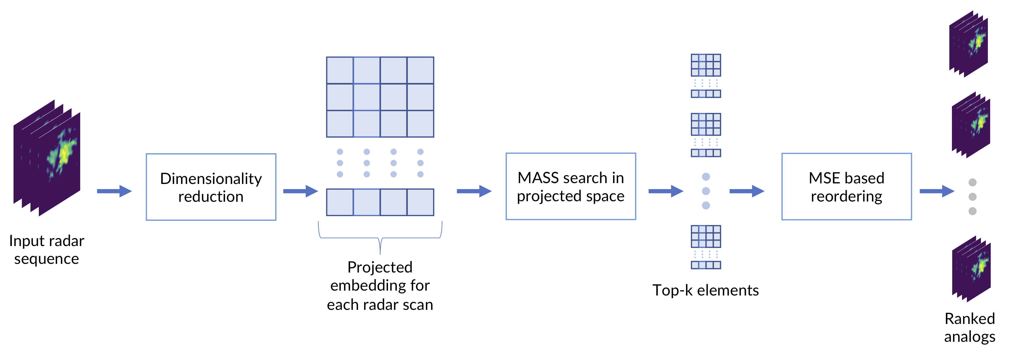
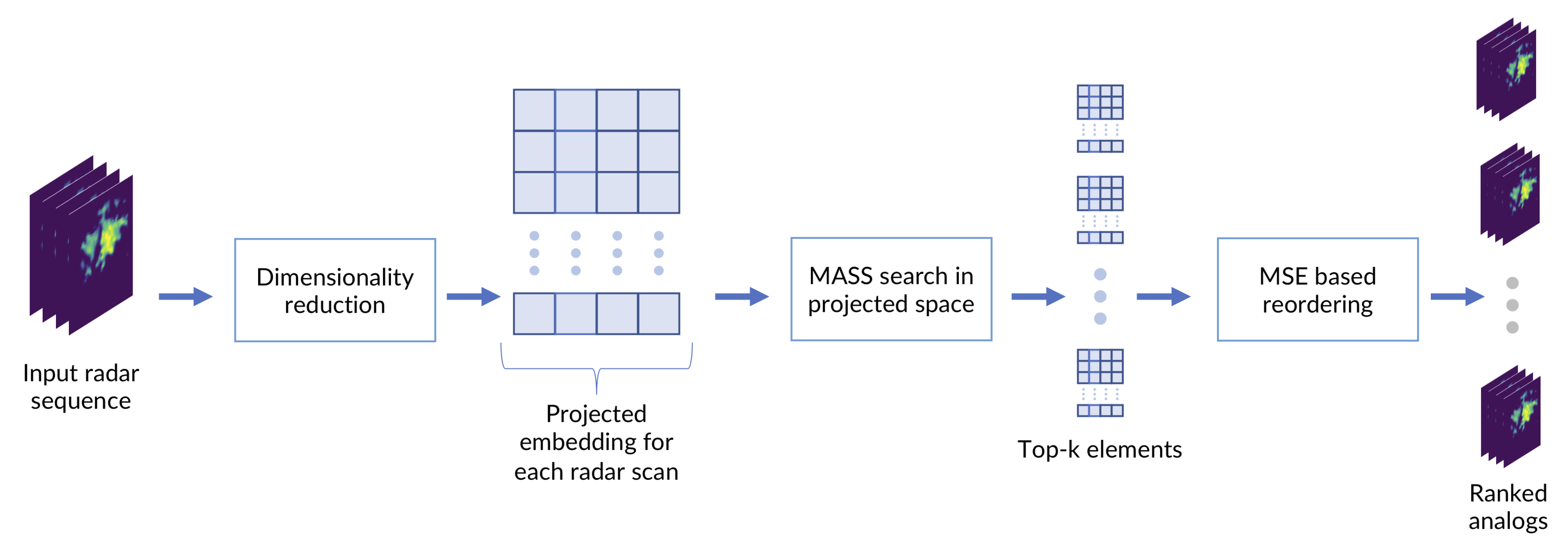
The second phase uses the MASS algorithm to search through the embedding search space and find the closest matches for the query data. To this aim, the embedded vectors of all the images in the search space are concatenated together following their natural time order. The result is a vector of length × . The embeddings of the queries are concatenated in the same fashion, generating vectors of size × t for each query, where t is the time length of the search query (the number of images in the sequence). The MASS algorithm is used to compare the query vector with the search space vector and extract the indexes of a desired number k of closest Euclidean profiles. The use of the Euclidean search is possible because the embeddings are projected by UMAP into a geometric space. As last step, the image sequences corresponding to the indexes of the top k profiles are compared and reordered by computing the MSE with respect to the query image sequence (in the low-res 64 × 64 image space), generating the final analog ranking. The desired number of final analogs can be selected by slicing the MSE reordered k analog vector to the final desired size of top-a analogs, with . There are two reasons why performing a partial reorder of the top k results in image space before selecting the final analogs is useful: first, even if the dimensionality reduction method works ideally on all cases and always returns the same top k items that an MSE search (the expressions “MSE search” and “MSE reorder” in the text, are always to be considered as operations computed by comparing radar images in the low-resolution 64 × 64 image space) would, there is hardly any guarantee that those will be returned in the same order (this is discussed in Section 2.6 and Section 3.2). The second reason is that MASS can perform such a fast search because it compares the vector profiles in the frequency domain; although the computed rankings for the profiles are exact, it may match a sequence with a very similar profile of the query vector but with a constant shift on all coordinates. This is indeed a rare occasion, but the partial MSE reordering is overall useful to move those spurious matches at the bottom of the ranking. Therefore, although we want to avoid computing MSE between the query and all the image archive, we can afford a small configurable number of MSE comparisons that can greatly improve the quality of the final ranking. The scheme of all steps of the workflow is summarized in Figure 2.
In an ideal setting, we want the embedding length d to be as small as possible (to reduce the memory requirements and the search time) and keep k as close as possible to a, to minimize the computation needed by the partial reorder step. For these reasons, we tested the performance of our method with different values of k and d with regard to the ability to return analogs in the same order that an MSE search would.
2.5. Evaluation Framework
To better highlight the contribution of the two phases to the overall result, we divided our evaluation in two parts. In the first part (Section 2.6) we evaluate the impact of dimensionality reduction methods (UMAP at different parameter configurations and PCA) on finding analogues in terms of MSE on single images. We assessed this ability using two different metrics (Section 2.6.1 and Section 2.6.2). In the second part (Section 2.7) we used MASS in conjunction with the best performing dimensionality reduction models, to test the ability of the overall solution in finding analogs of different length (t), using the error computed with respect to sequences found by MSE search in the original (64 × 64 pixels image) space as ground truth. Computational and memory requirements were also considered.
2.6. Evaluation Part I: Dimensionality Reduction Training and Verification
In Section 2.1, we discussed the four parameters driving the UMAP dimensionality reduction algorithm. For the purpose of this study, we are especially interested in testing two of them: number of components d (that corresponds to the embedding length) and number of neighbors n. Default settings were used for the two other parameters (metric = Euclidean and ). The rationale for this choice is that for the aim of analog retrieval we were not interested in the absolute distance values, but our objective is to keep the same ranking distance between the elements in the original and the embedded space. This means that any distance function that preserves ranking with regard to MSE can be used, such as the default Euclidean distance used by UMAP. The same holds true for the minimum distance between the points where the projected data will lie. This allowed us to concentrate our effort on the remaining parameters where we chose to setup a grid of six values for and 6 values of for the model optimization.
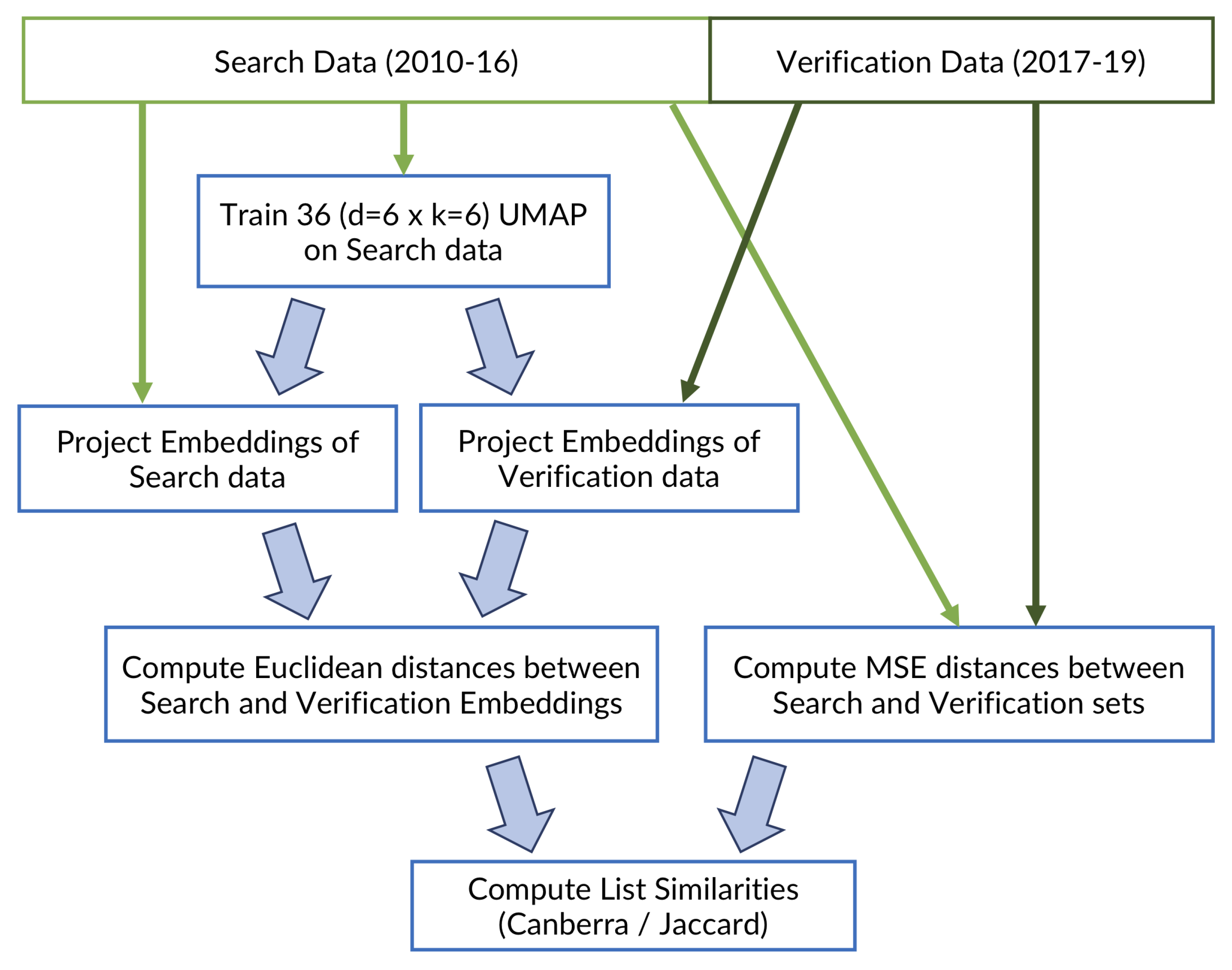
Using as input the whole set of search data, we fit 36 UMAP transformations with different parameters, given by the cartesian product of six choices of d and n. We then proceed to produce the embeddings of all the UMAPs for both the search data and the query data.
To evaluate the impact of UMAP to preserve rankings, we took the daunting task of computing the MSE distance matrix between all the images in the archive vs all the images in the query set, thus generating a matrix of distances. This matrix allowed us to create an extensive and accurate verification setup of the ability of UMAP to rank and find the same analogs compared to MSE, considering different thresholds of top k elements.
Figure 3 illustrates the workflow of the UMAP model training and verification.
As a baseline comparison method, we considered the embedding space generated with Principal Component Analysis (PCA) [19]: its use as dimensionality reduction technique for radar analog search has been proposed in [16]. Like UMAP, the PCA embedding maps the original space to a geometric space, so we can use Euclidean calculation to compute the distances. All the steps described for UMAP were applied also for PCA with only two notable differences: first, we had to train only one configuration, as PCA is nonparametric; second, we had to apply more normalization steps to our data archive before computing the PCA, because of the variance maximization used to find the principal components is extremely sensitive to unbalanced values. For this step, we followed the same workflow described in [16]: we applied Box-Cox transformation [28] adding a 0.01 offset to the rainfall rate of each radar scan, and centered each element by removing the corresponding mean before computing the PCA.
We tested all the trained dimensionality reduction configurations methods by introducing two evaluation metrics that helped us to measure the characteristics of the ranking results returned by UMAP/PCA against the ideal rankings found via MSE. The first metric is a weighted ranking correctness measure (Section 2.6.1), the second measures the proportion of correct elements found in the nearest top k (Section 2.6.2).
2.6.1. Stability of Ranked Lists
The Canberra stability indicator [29] is a group-theoretical measure for assessing the similarity of a set of ranked lists of n shared items. The indicator is based on the Canberra distance [30], a weighted version of the L1 norm whose main features is to penalize more the differences occurring in the top part of the ranked list rather than those occurring at lists’ bottom. The indicator is normalized by the expectation E of the Canberra distance on the whole permutation group of cardinality , so that , with denotes a set of very similar lists, whereas indicate that is a randomly ranked set of lists [31]. By using the locator parameter k [31], the same measure can be restricted to evaluate the similarity of the top-k sublists of including only the highest ranked items. We used this measure to evaluate how well the top k embedding elements are ranked compared to the MSE ranking.
2.6.2. Jaccard Distance
The Jaccard distance is a dissimilarity measure between two sets. The Jaccard distance () is the complementary of the Jaccard index (J) [32], and it is defined as
where A and B are two set of elements and ∩/∪ are the intersection/union operators.
Intuitively, this distance helps to understand what is the proportion of items that are present in both sets, normalized by the total number of distinct elements. A value of is obtained between two identical sets, whereas a value of corresponds to two disjoint sets. We used this measure to evaluate how many of the top k elements found by searching the embedding space corresponded to elements returned by the top k MSE search. The comparison is also useful to assess and compare the performances between PCA and UMAP for analog retrieval. As with the Canberra stability indicator, the Jaccard distance is used to evaluate the similarity of the top-k sublists of .
2.7. Evaluation Part II: Sequence Search Evaluation
In the second part of the evaluation, we assessed the complete workflow: we combined UMAP and MASS to test the retrieval of analog sequences of different lengths (t) and different number of top-k sequences. For this part, we evaluated the solution by comparing the straight cumulative MSE error between the sequences found by MASS-UMAP and MASS-PCA and the sequences retrieved by MSE. We found this comparison to be a more faithful representation of the performances of the overall solution than using the two metrics introduced in part I. Indeed, as the testing occurs with sequences of different lengths, the total number of possible matches available between the query data and the archive is different for every value of t: this makes the interpretation of the metrics much less straightforward. We also benchmark the use of computing resources required both theoretically and experimentally. Wall execution times are reported when available and discussed.
3. Results
3.1. Exploration of UMAP Embeddings
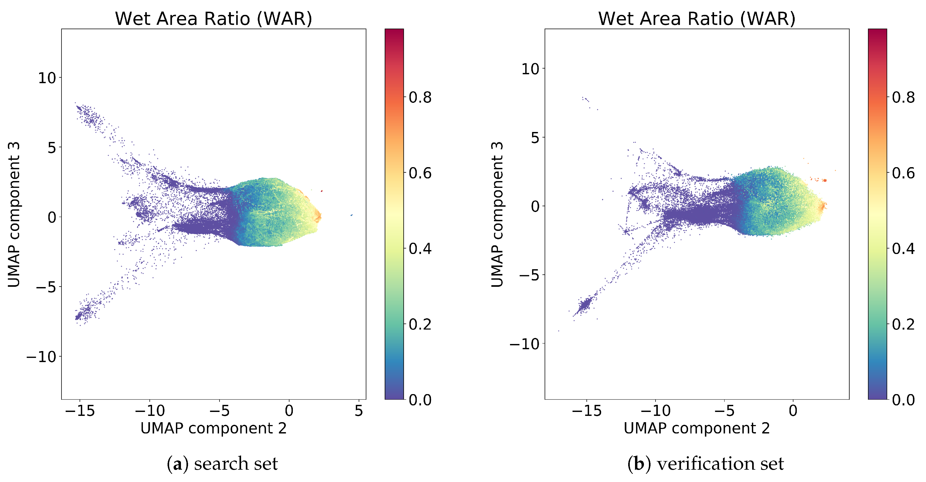
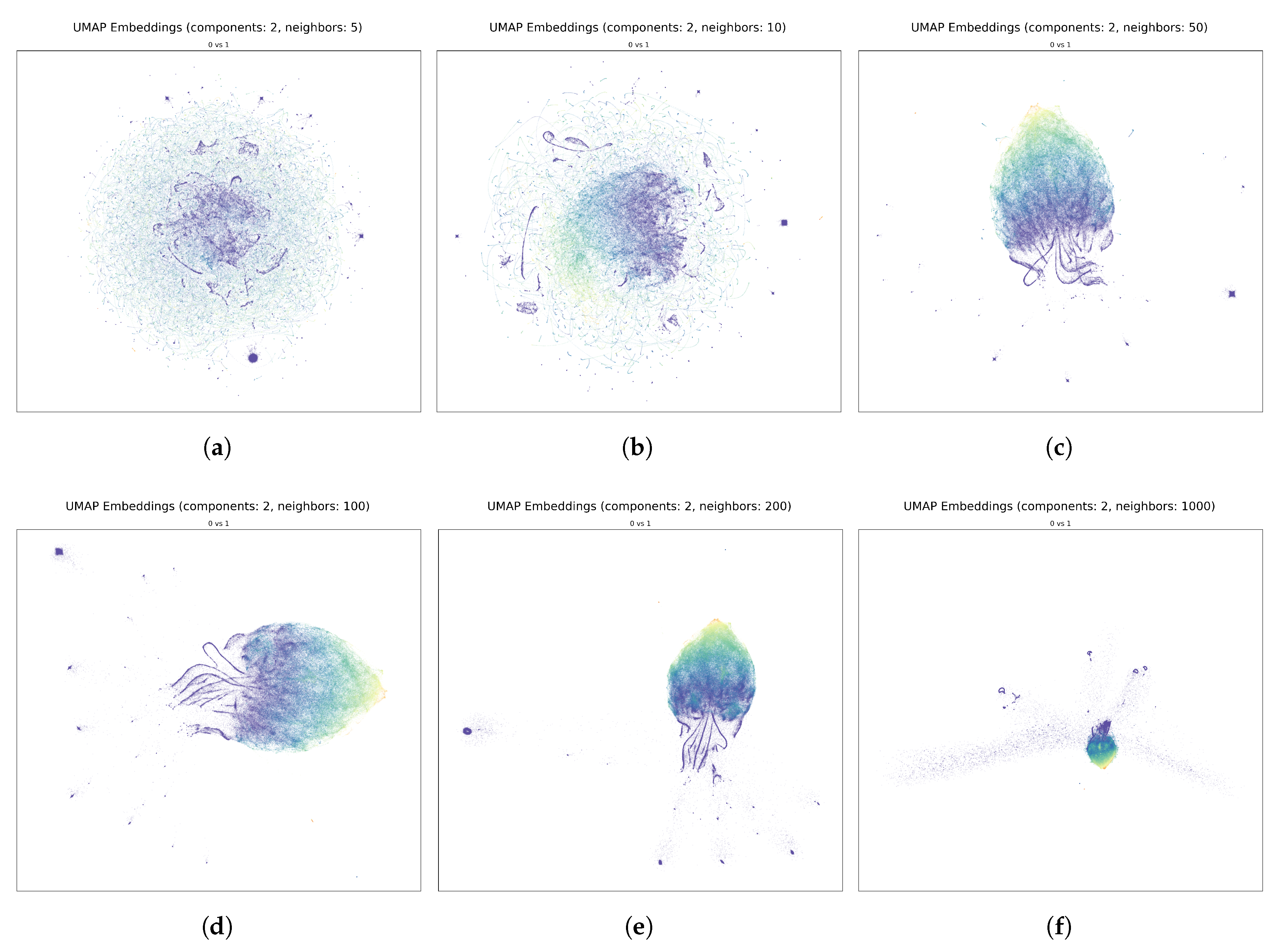
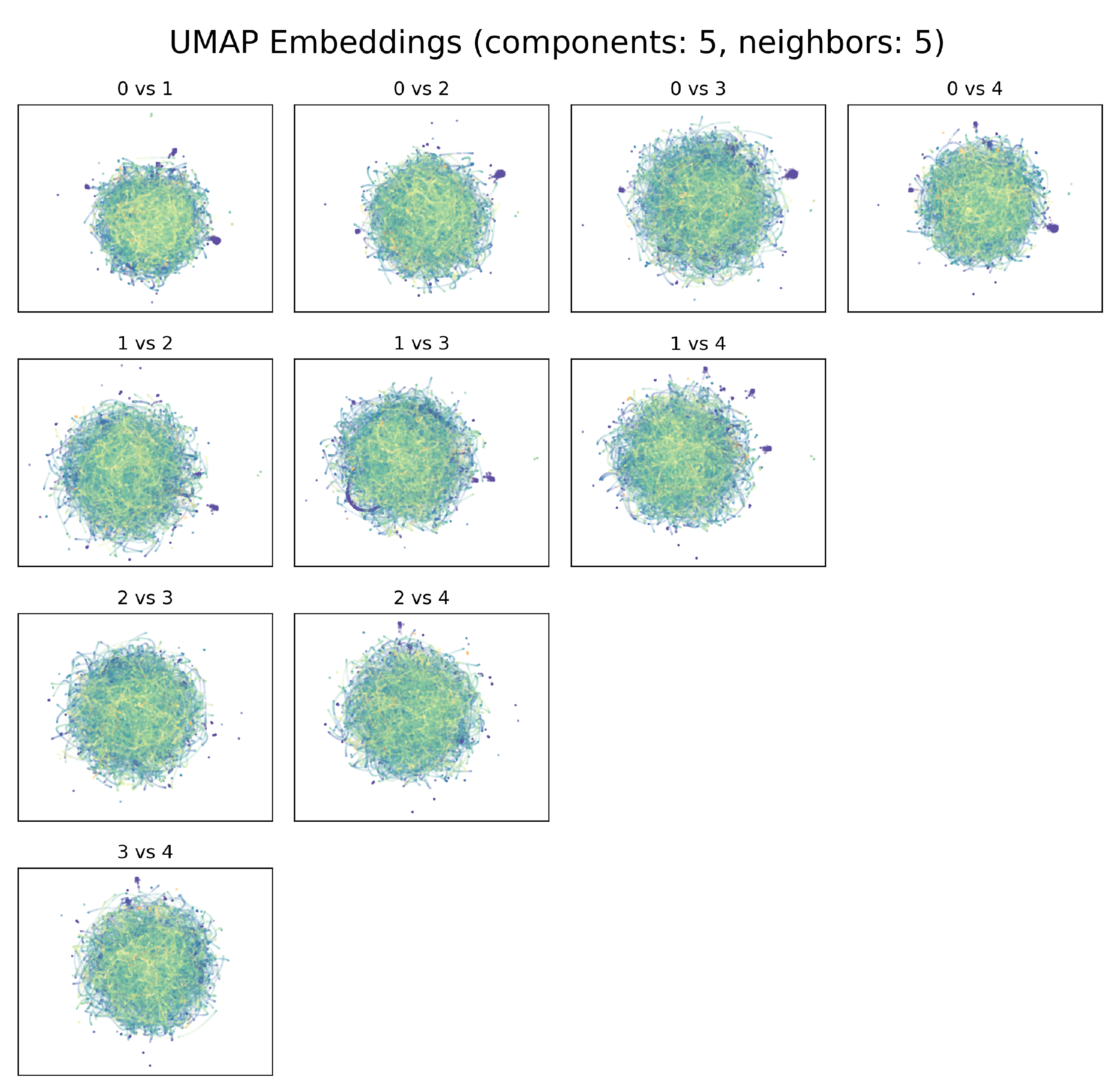
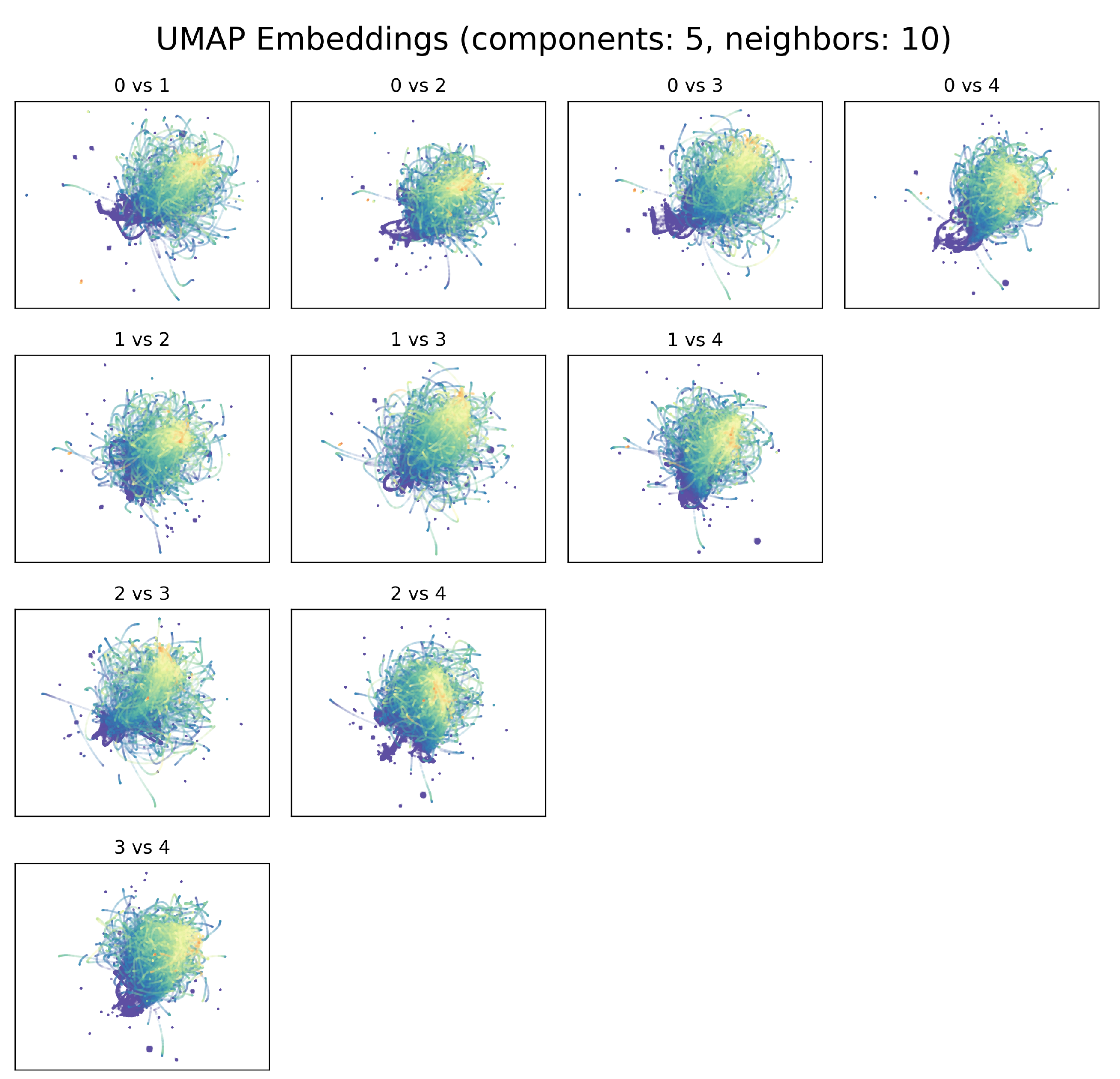
We investigated some of the manifolds generated by UMAP projections and plotted the resulting embeddings for the search and the verification sets (Figure 4). The hyperparameters for the represented model are the one found for the best model in Section 3.2, with number of components and the number of neighbor . If we consider for example the second and third components, the visualization of the two embeddings belonging to the search set (on which the UMAP is constructed) and the verification set are quite similar, where the embedding points are colored by the Wet Area Ratio (WAR), defined as the percentage of pixels with a rain rate higher than mm/h. The stability analysis shows that UMAP is able to project the space maintaining the general distances between radar scans with different rain rates. Notably, the two sets are composed of radar scans collected from 2010 to 2016 for the search set, and from 2017 to 2019 for the verification set. UMAP generalizes well across the two years, and it is applicable to scans from future time windows without the need for retrain.
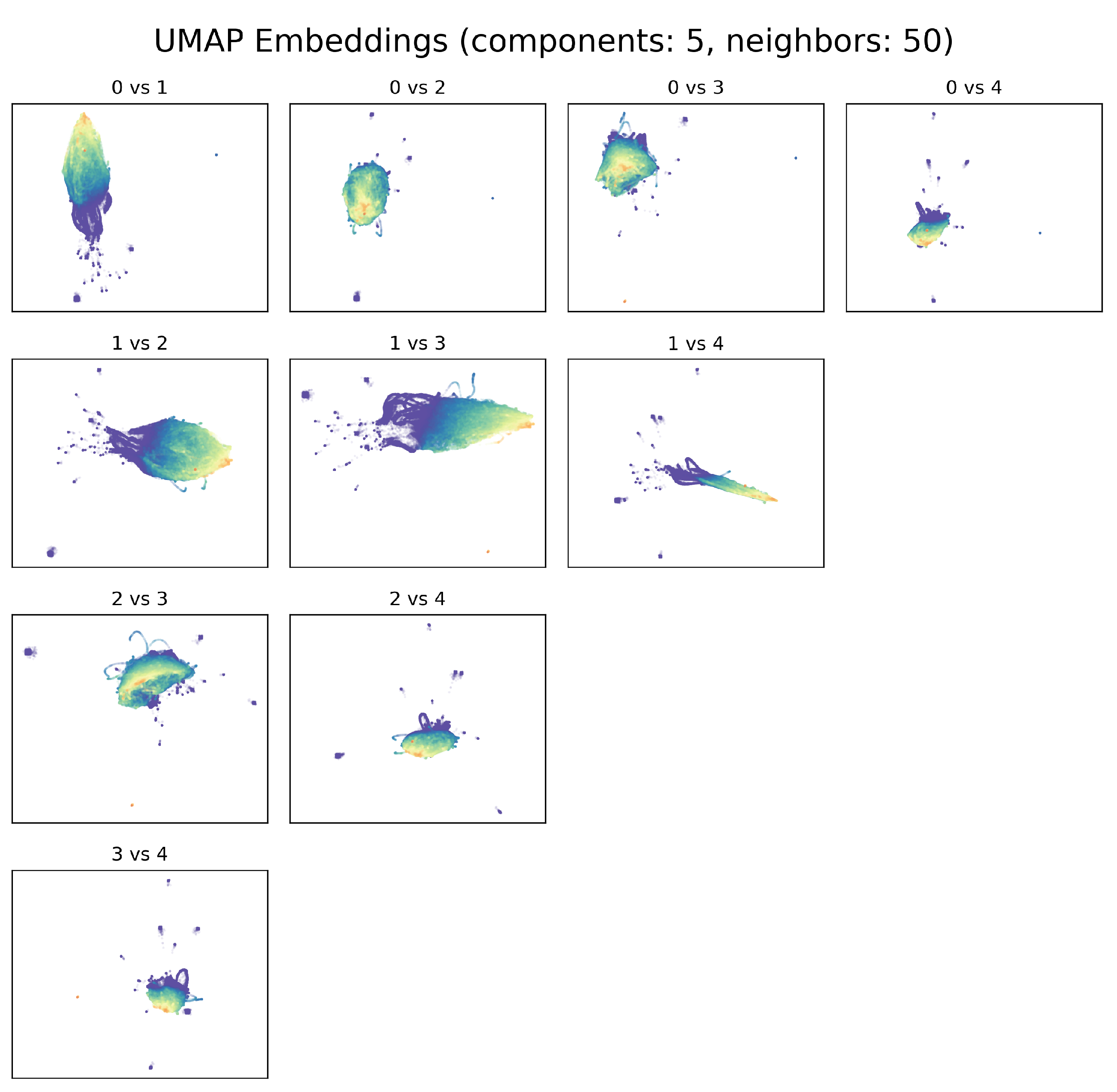
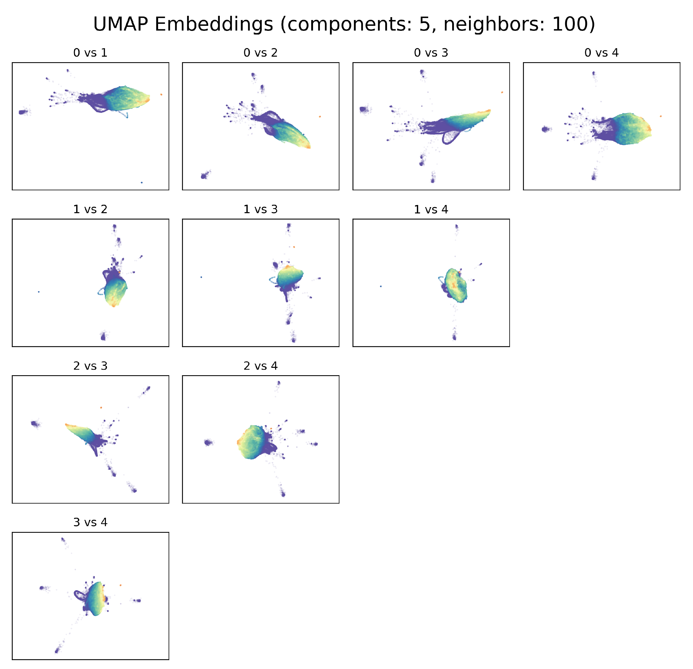
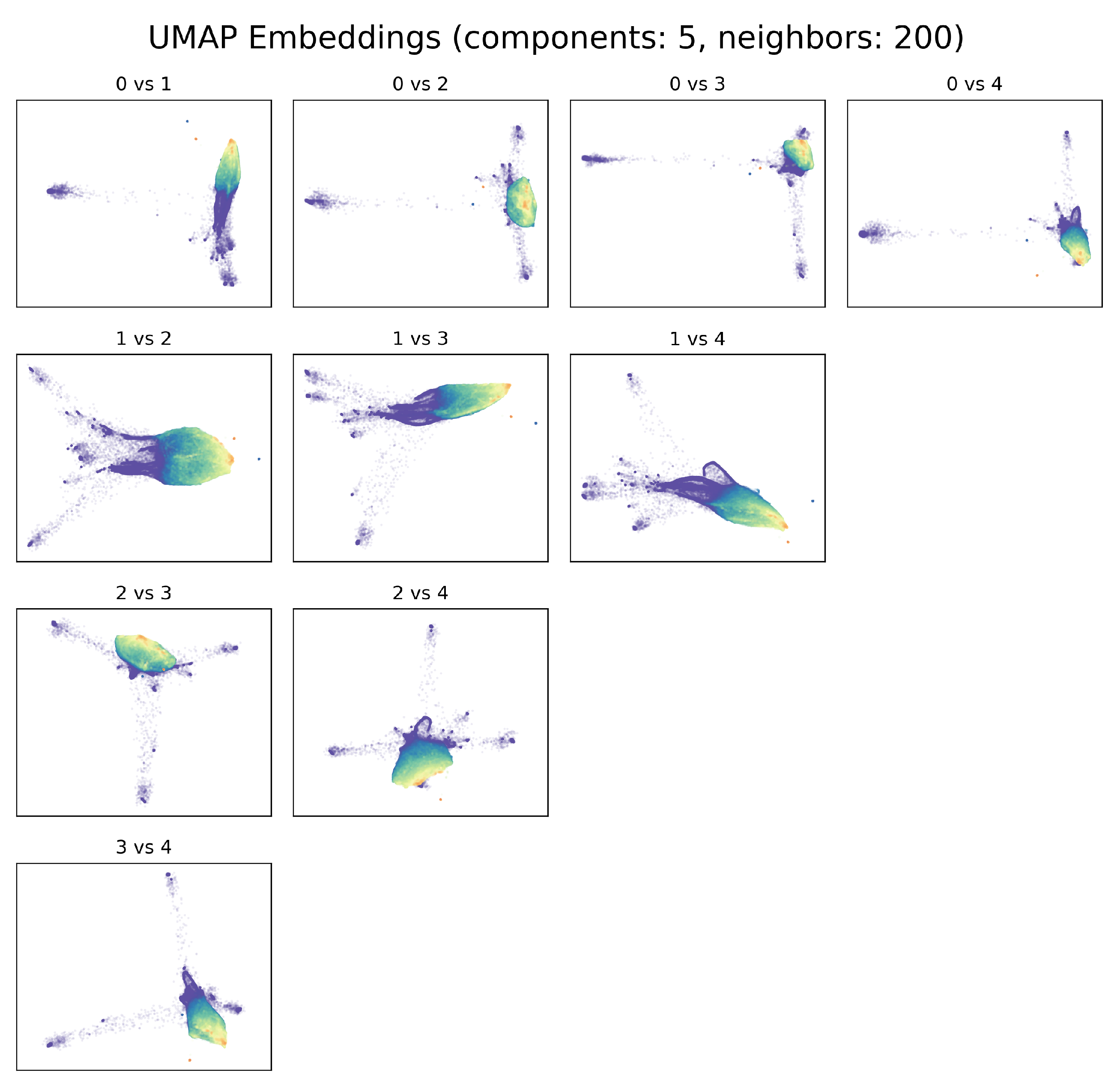
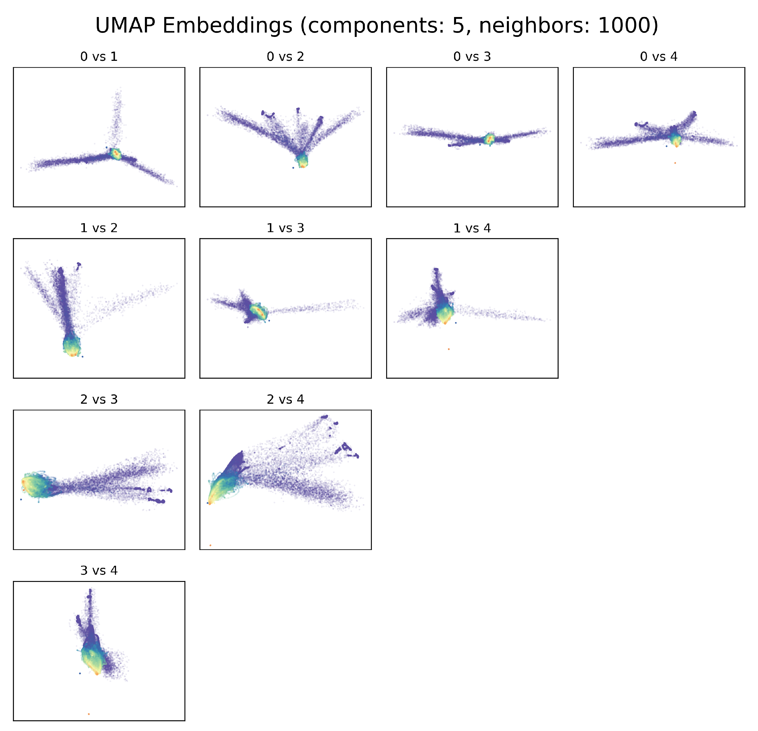
In Appendix A.2, we report the plots for several configurations of UMAP and we show the impact of different choices of number of components and neighbors on the radar dataset.
3.2. Evaluation Part I: Dimensionality Reduction
The evaluation of the dimensionality reduction step was implemented as explained in Section 2.6. Thirty-six UMAP configurations were fitted on the search data, and the embedding of both search and verification data were generated. The UMAP embeddings were used to compute on the fly the ranking distances for all the verification images and compared with the MSE ranking to compute the cardinality of the set intersections and the Canberra indicator for a number of top-k results. The average and standard deviation for Jaccard and Canberra distances on all validation images were then computed for all possible permutations of k (limits), d (components) and n (neighbors). The final number of computed results is given by the cross product of the configuration space built with the following parameters.
- limits: with configurations
- components: with configurations
- neighbors: with configurations
The total number of parameters tested for the UMAP projection is . Conversely, for PCA the size of the tested configuration space was , where D is mapped to limit the number of principal components used by the PCA decomposition to the same number of components of UMAP.
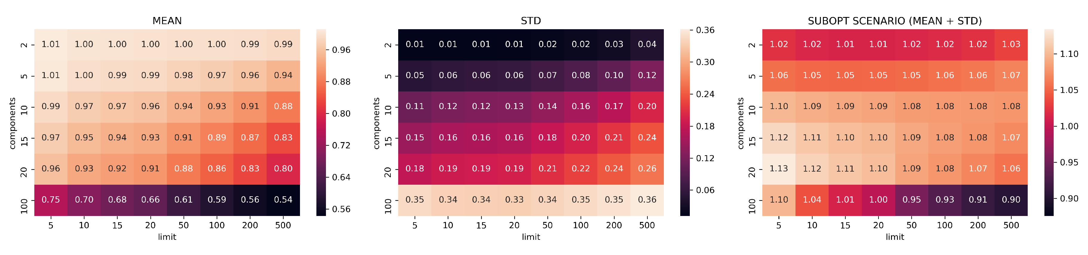
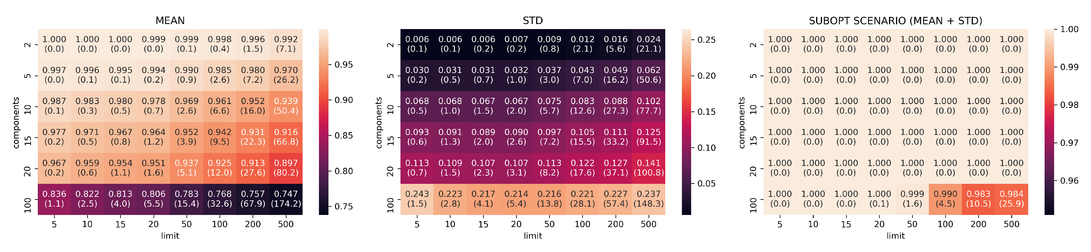
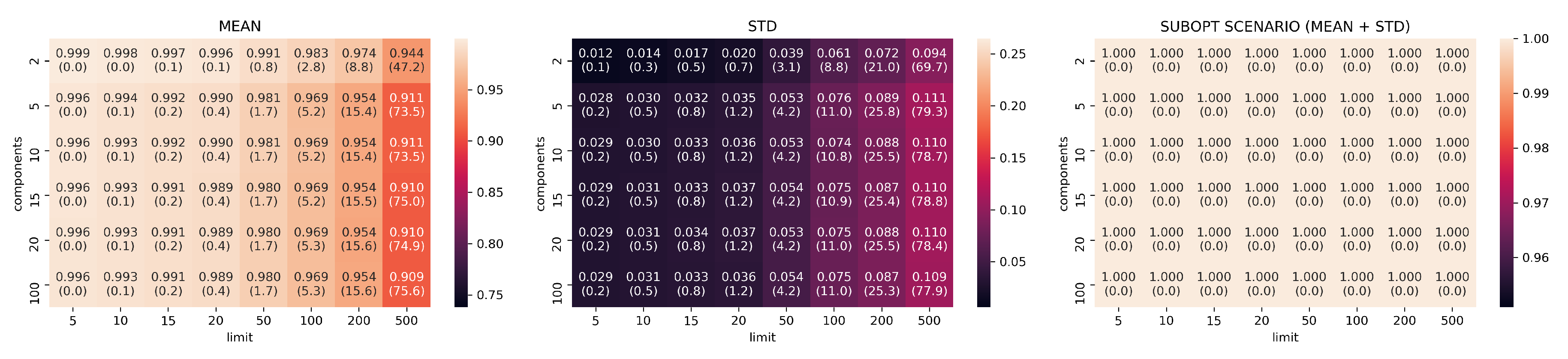
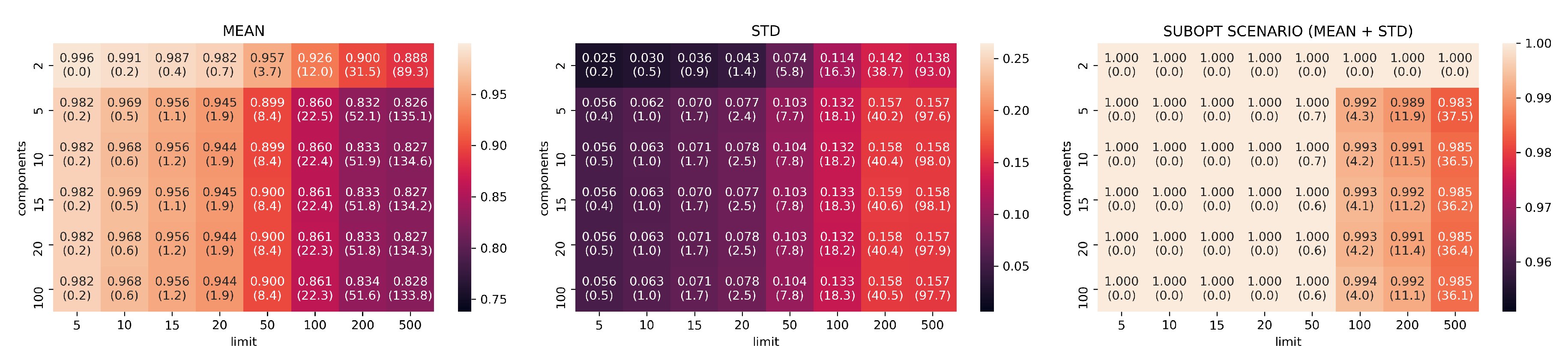
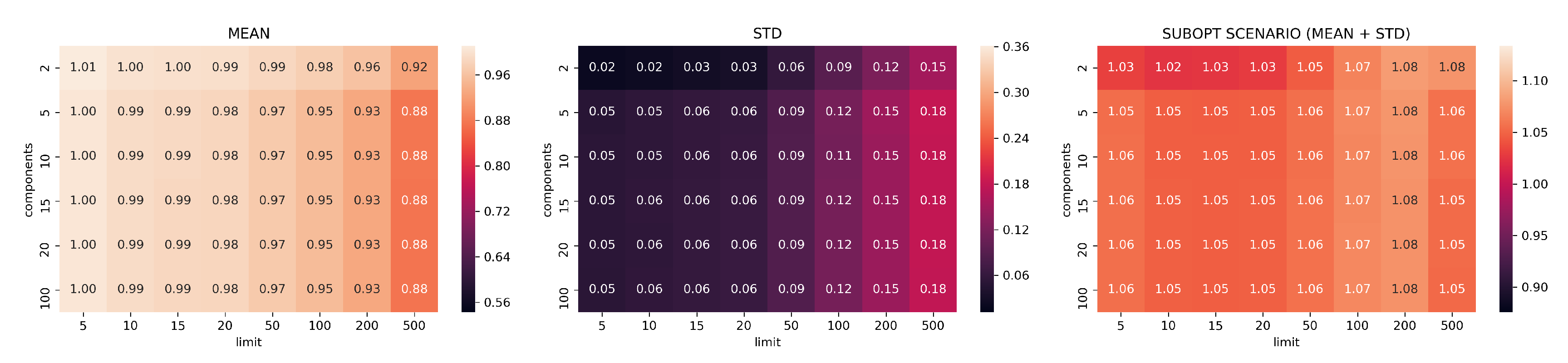
The results of the 48 configurations tested on PCA are reported in Figure 5 for Canberra stability index and in Figure 6 for Jaccard. For each configuration we group together the means, the standard deviations, and the suboptimal scenario, namely, the sum of mean and standard deviation, describing the retrieval performance of the dimensionality reduction with suboptimal results.
Reduction by PCA is consistent and predictable: it shows systematic linear improvements in both Canberra and Jaccard metrics by adding more components and extending the size of top-k considered elements. On the other hand, PCA needs to use at least 20-components and 500 top-k elements to start showing consistently good ranking results (an average of 80 elements in common with the top 500 MSE elements).
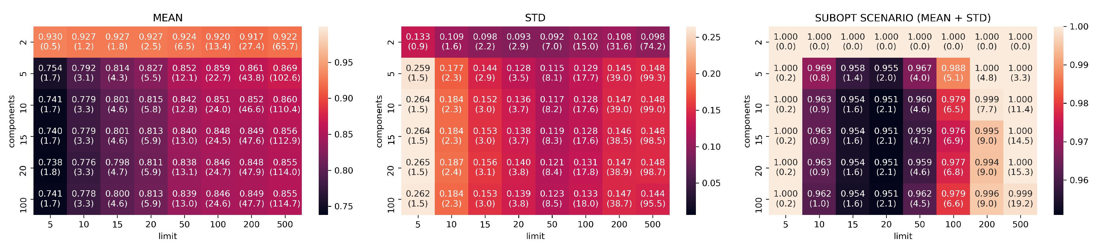
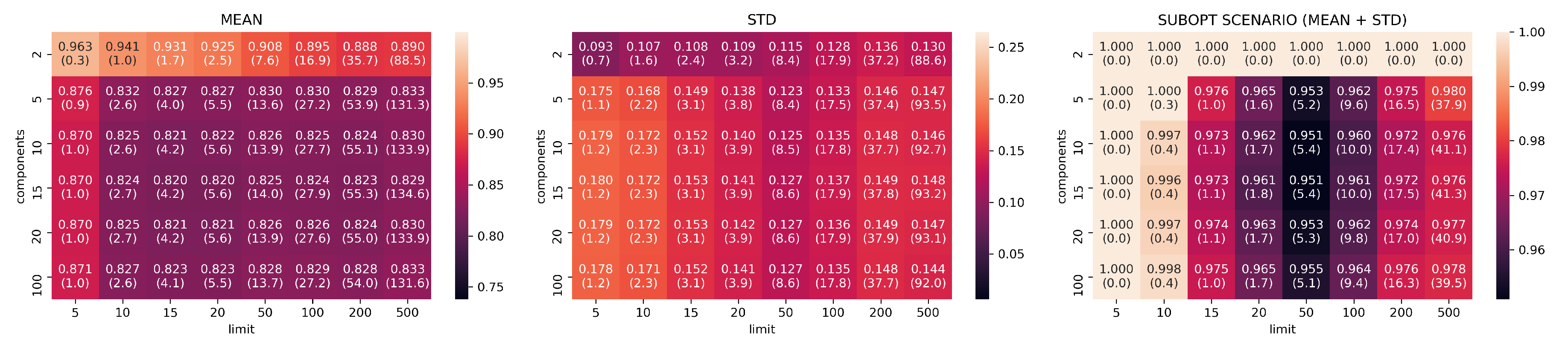
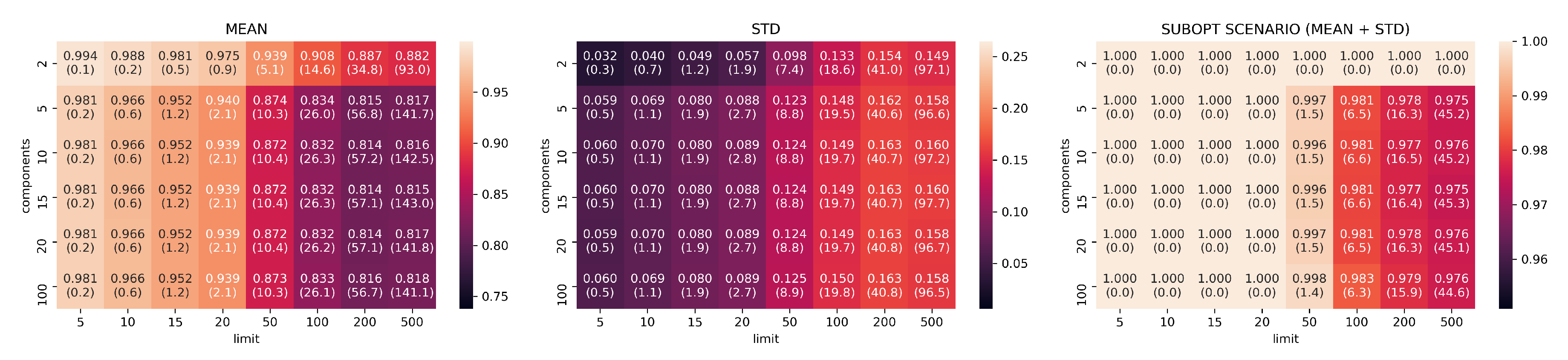
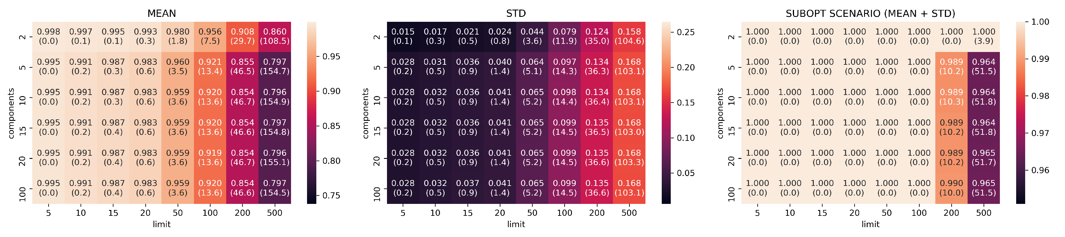
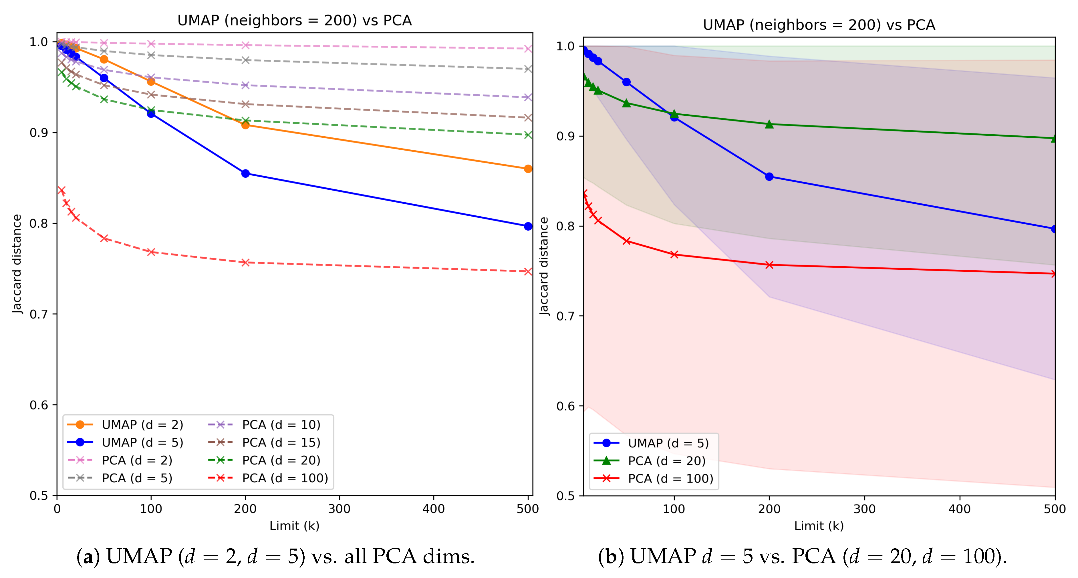
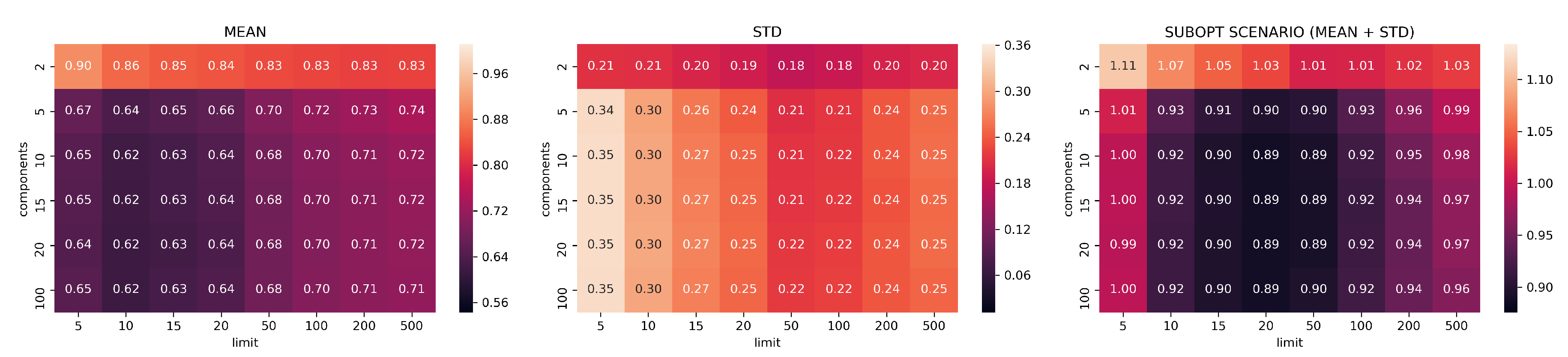
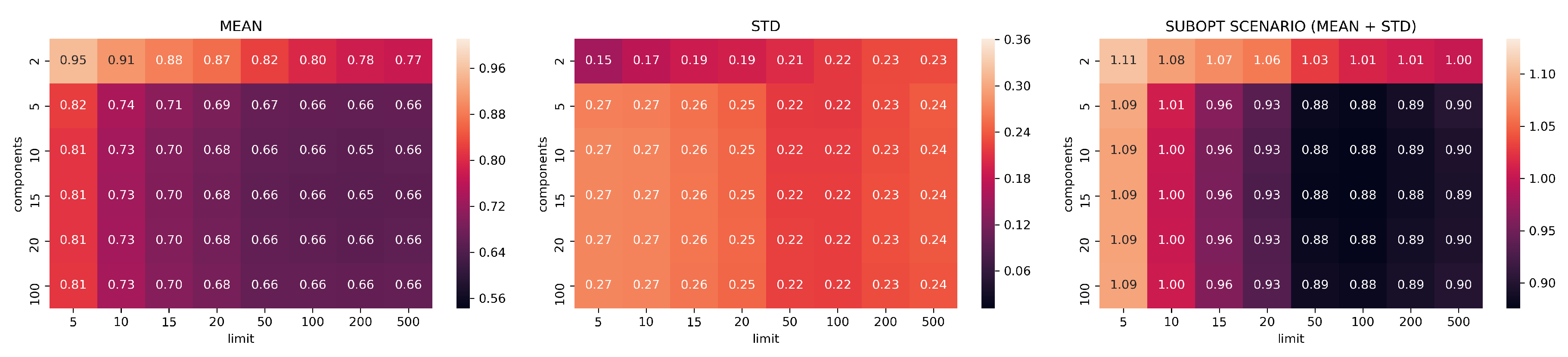
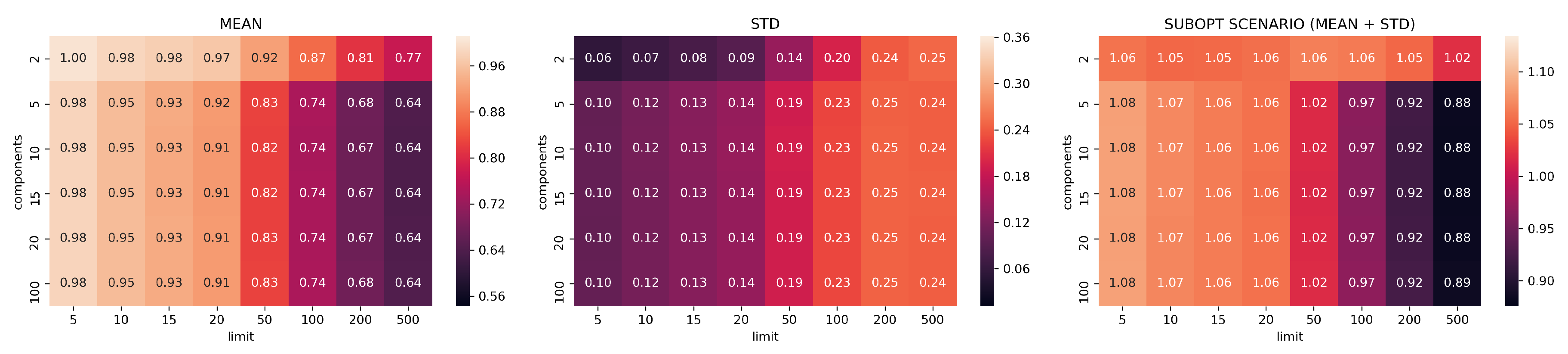
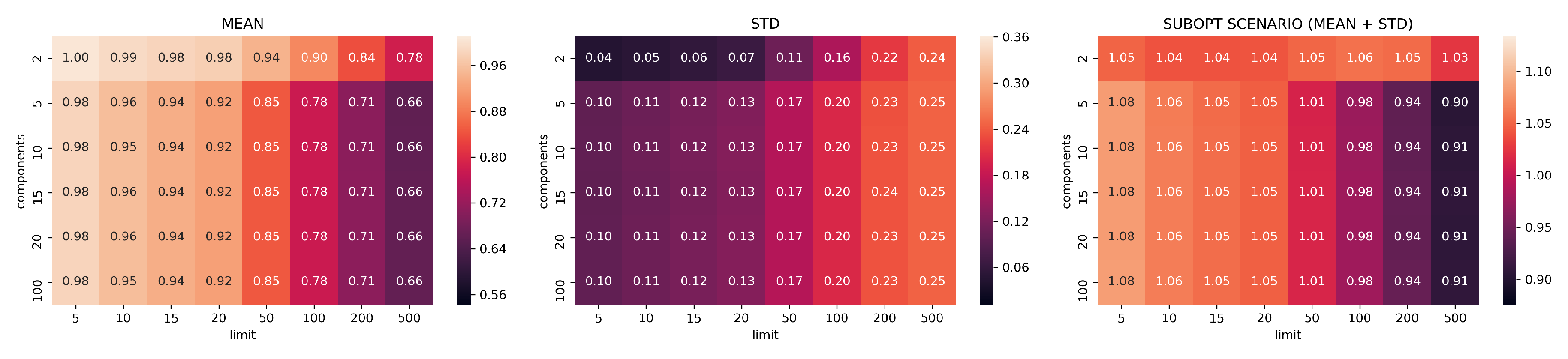
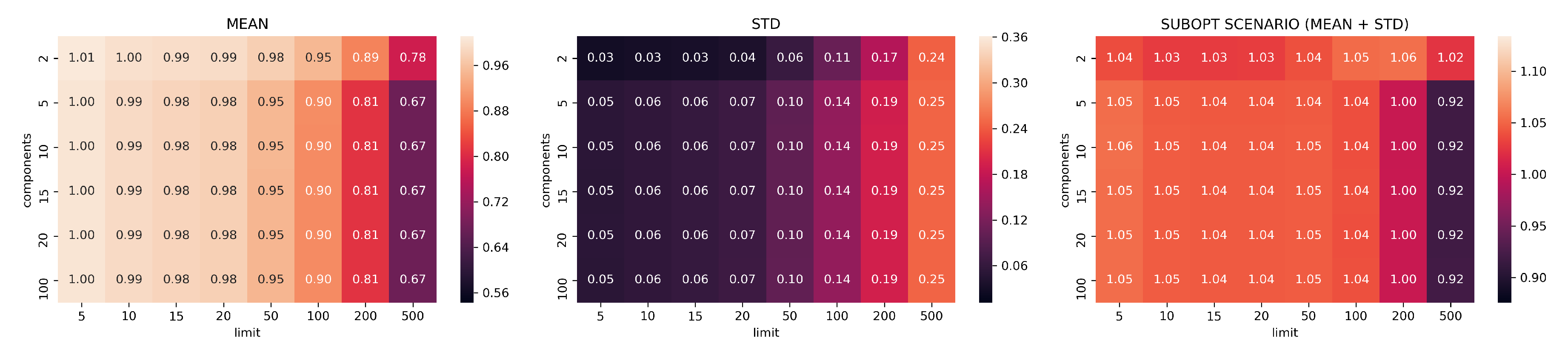
In Figure 7, Figure 8, Figure 9, Figure 10 and Figure 11, the analysis of search reduction by Jaccard distance for different values of n of UMAP are reported. The first observation is that UMAP does not follow a linear trend: the algorithm improves dramatically ( 40%) between 2 and 5 components, to then subsequently plateau. Going from 5 to 100 dimensions makes hardly any difference in the ability to find better analogs, and this behavior is consistent even with different values of n. Thus, we conjecture that this saturation in the dimensionality is dataset dependent, and that UMAP has already maximized its ability to describe the data manifold using 5 components. On the other hand, choosing a different value for n drastically changes the performance of UMAP with regard to the choice of k. The two values appear to be positively correlated: to train a transformation that finds a consistent number of good analogs in the top-k, we need to set n around the value of k (usually a step lower).
Given the consistently good results that UMAP showed using just five dimensions and the positive correlation between n and k, we choose the configuration with , , and as a benchmark for the second part of our evaluation. Figure 12 summarizes the findings for the chosen values. In Appendix A.1, we report the plots for all the remaining configurations not included in this section.
3.3. Evaluation Part II: Spatiotemporal Analog Search Performance
3.3.1. Analog Quality
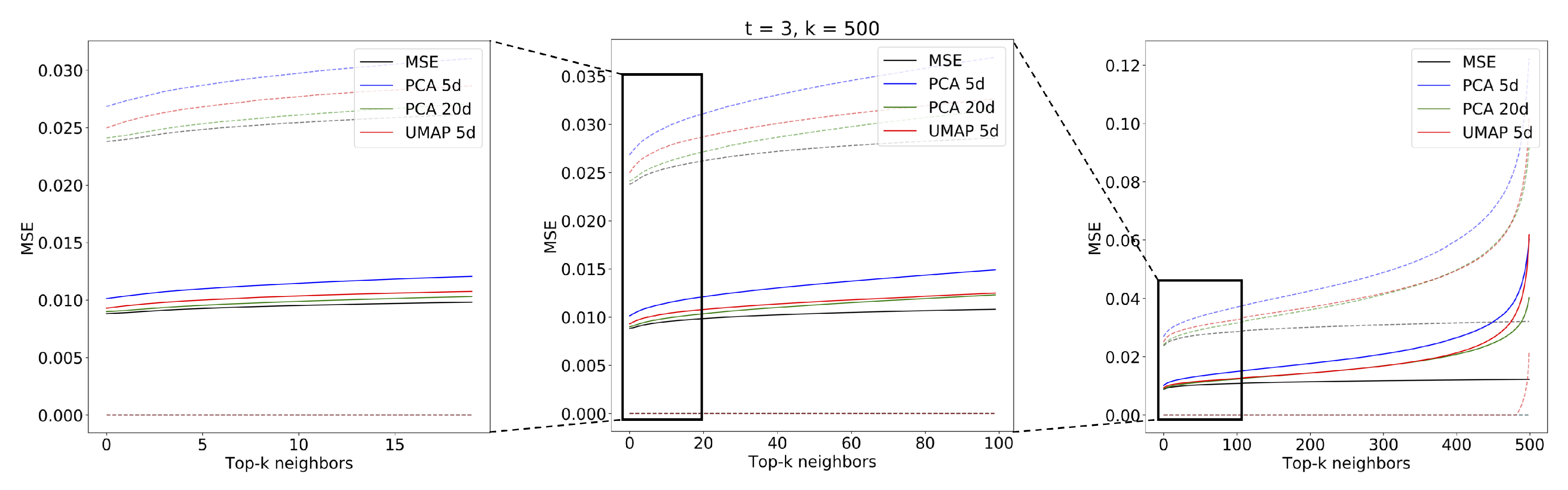
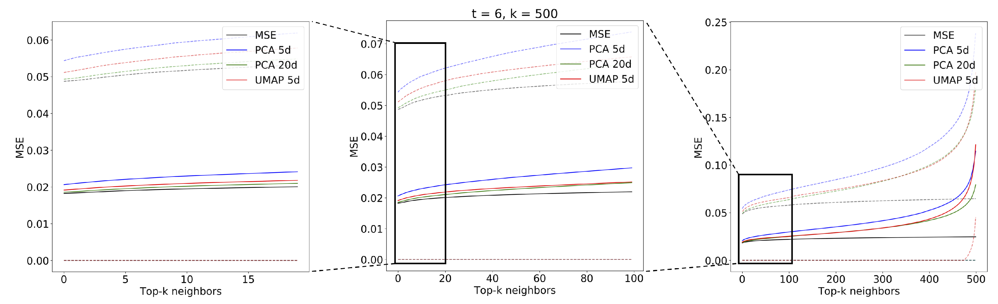
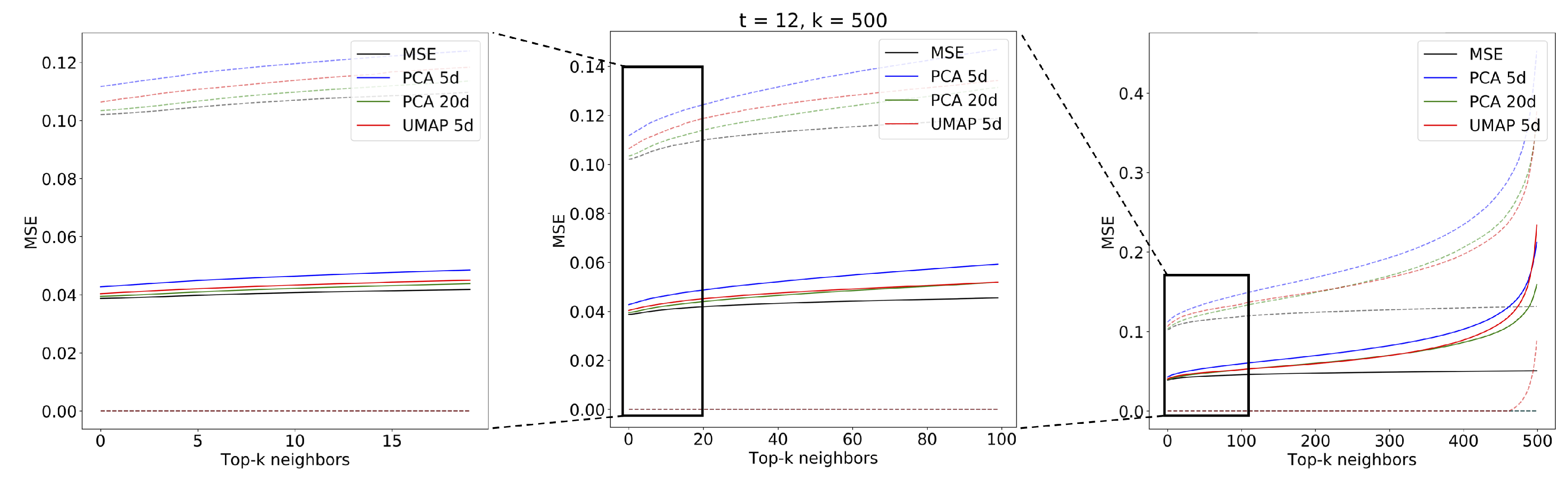
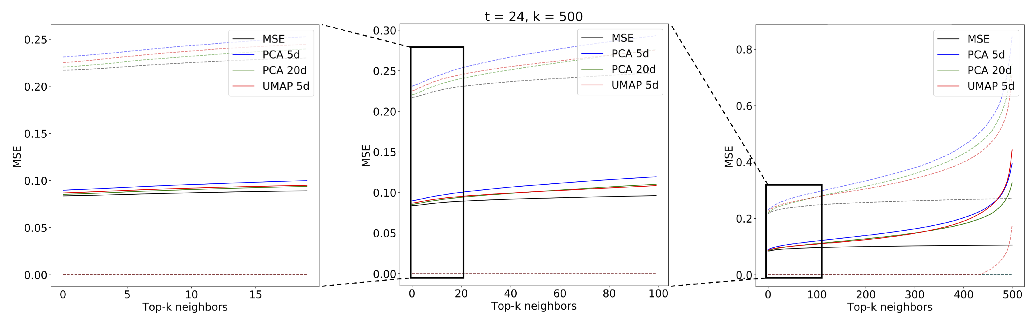
The evaluation of the spatiotemporal analog search performance was implemented as explained in Section 2.7. We used the combination of UMAP and MASS (MASS-UMAP) to find analogs for sequences of different lengths. We tested values corresponding to sequences of 15, 30, 60, and 120 min, respectively. For comparability, we used the same number of sequences with the same start times for all values of t. The sequences were chosen from the query set, starting from the first index and leaving whenever possible 100 images of gap between the beginning of the next sequence: this avoided sequence overlapping and also such a gap was sufficiently long to guarantee complete spatiotemporal decorrelation between the chosen sequences. The total number of extracted sequences after such processing was 1226. We compared the best UMAP configuration (, ) with respect to the sequences found by MSE and the sequences found by PCA with 5 and 20-components. Figure 13, Figure 14, Figure 15 and Figure 16 show the mean MSE of the models with different values of t and a MSE reorder on the top elements.
The figures show the plot of the average MSE error between the query sequences and the top sequences for each i-th analog in the ranked list. The results are consistent with the performance on single images: the 5-component UMAP consistently outperforms 5-component PCA on all T by a wide margin. The UMAP results are actually on par with 20-component PCA, where UMAP accounts for slightly higher MSE error for and an lower for and . Results of the top two most similar sequences found given a query sample (Figure 17) of radar scans are shown for the three compared methods: using MSE on the original scans (Figure 18) and using MASS and MSE-based reordering on the top-500 closer embeddings on PCA (Figure 19), and on UMAP (Figure 20) embeddings.
In Appendix A.3, we discuss the effect on analog quality when using different query lengths (t).
3.3.2. Execution Times and Memory Requirements
We tested the execution times of MASS-UMAP on our dataset first by benchmarking each component of the method separately and then by executing the whole workflow end to end. Table 2 shows the result of our benchmarking. The UMAP configuration chosen for the test is the same used in Section 3.3.1 with parameters , and .
All reported tests were executed ten times; confidence intervals are reported. The test platform used was a non-burstable cloud instance with processor Intel(R) Xeon(R) E5-2673 v4 running at 2.30 GHz and 425 GB of RAM. For a fair comparison, all algorithms were executed in single thread mode. The speedups given by MASS-UMAP against linear MSE search were computed by preloading all the image archive and query images in memory, so the reported results for the linear MSE search are the fastest possible, with no disk access. Although this approach is useful for testing purposes, in real applications, this is usually not possible because of memory limits or operational choices, and thus the gap between MASS-UMAP and MSE search will skew even more in favor of the former because of less or no needs of disk access. We remark that the entire archive and query embeddings can fit in 342,598 × 5 × 4 bytes = 6.5 MB of memory, while the original radar scans account for more than 5 GB of data even after the 64 × 64 pixel resize.
4. Discussion
The MASS-UMAP method proved to be a flexible and effective method: it not only allows for searching analog sequences of arbitrary length in a few seconds over several years of data archive, but it also improves accuracy over published results [16]. Although in this work we focused our analysis only on the minimization of MSE as objective, any positive distance measure can be used to tune the UMAP dimensionality reduction. An example of this would be using a distance measure that is robust to a certain degree of rotation or translation, like the Complex wavelet structural similarity [33], allowing finding analogs accounting for a certain degree of displacements or rotation [14]. The MASS-UMAP method allows also the integration of external variables: synoptic or seasonality descriptors can be integrated by concatenating the desired variables to the UMAP embedding generated for each image and weighted during MASS search. We also envision the possibility to test functions different from Euclidean distance to search the projected space. Finally, the UMAP neighbors parameter n allows to derive the embedding distribution that fine tunes the search results for a specific number of top k analogs. We believe that our verification setup was extensive enough that our findings about the optimal values of d, n and k can be reused as baseline parameters at least for other radar datasets, but we envision the use of the method also for any other remote sensing applications where spatiotemporal search is needed.
The drawback of our solution is that its flexibility comes with a price: some combination of parameters can give worse result than PCA. To avoid these edge cases, a proper verification like the setup proposed in this paper is needed. We show UMAP gives substantially better results than PCA on all reasonable number of dimensions in this setup. The same warning holds for MASS: to avoid search results with spurious matches we provide the top-k MSE reordering mechanism to filter spurious matches as analogs. Another aspect that could be investigated is the effect of the use of different spatial resolutions in the training of UMAP: although the image resolution we used was sufficient to describe the variability [34] for the general task we presented, specific applications may require the use of radar images at higher resolution, for example to characterize specific type of precipitation in convective rain cells.
As future research directions we plan to use this methodology as an operational application in probabilistic precipitation nowcasting. Another possibility we envision the usage of ensembles of UMAP trained with different configurations and metric functions to improve the retrieval of analogs in embedded space.
5. Conclusions
In this work, we presented an approach to reduce the computational complexity of analog search. Instead of computing the MSE between a search query and the whole historical archive set we demonstrated the efficiency of a combined approach based on three steps: dimensionality reduction, fast search in constant time in the embedding space with MASS and MSE-based reordering on a subset of potential candidates, reducing the computational burden by a factor of 20. We also assessed the performances of MASS-UMAP when searching for sequences of different length. In addition compared UMAP against PCA, showing that UMAP can use a much smaller number of components, leading to superior performance and less memory requirements. These results make the MASS-UMAP approach appliable for nowcasting applications, where efficiency in finding analogs can lead to more accurate and precise predictions in very short time windows.
Author Contributions
conceptualization, G.F.; methodology, G.F. and G.J.; software, G.F.; validation, G.F. and L.C.; formal analysis, G.F.; investigation, G.F.; resources, C.F.; data curation, M.P.; writing—original draft preparation, G.F., L.C. and G.J.; writing—review and editing, C.F.; visualization, L.C.; supervision, C.F.; project administration, C.F.; funding acquisition, C.F.
Funding
Computing resources partially funded by the Microsoft Azure Grant AI for Earth “Modeling crop-specific impact of heat waves by deep learning” assigned to C.F.
Acknowledgments
We thank the Civil Protection Departments of the provinces of Trento and Bolzano for their help and their daily commitment in the maintenance of all weather data collection systems.
Conflicts of Interest
The authors declare no conflicts of interest.
Abbreviations
The following abbreviations are used in this manuscript.
| MSE | Mean Squared Error |
| PCA | Principal Component Analysis |
| UMAP | Uniform Manifold Approximation and Projection |
| MASS | Mueen’s Algorithm for Similarity Search |
| AnEn | Analog Ensemble |
Appendix A
Appendix A.1
Figure A1.
Jaccard results for UMAP models trained with neighbors .

Figure A2.
Canberra results for UMAP models trained with neighbors .

Figure A3.
Canberra results for UMAP models trained with neighbors .

Figure A4.
Canberra results for UMAP models trained with neighbors .

Figure A5.
Canberra results for UMAP models trained with neighbors .

Figure A6.
Canberra results for UMAP models trained with neighbors .

Figure A7.
Canberra results for UMAP models trained with neighbors .

Appendix A.2
Figure A8.
Example of UMAP Embeddings that show the effect of using different neighbors parameters (n) in two dimensions () on the training set, colored by wet area ratio.
Figure A8.
Example of UMAP Embeddings that show the effect of using different neighbors parameters (n) in two dimensions () on the training set, colored by wet area ratio.

Figure A9.
UMAP Embeddings of the training set colored by Wet Area Ratio for and .

Figure A10.
UMAP Embeddings of the training set colored by wet area ratio for and .

Figure A11.
UMAP Embeddings of the training set colored by Wet Area Ratio for and .

Figure A12.
UMAP Embeddings of the training set colored by wet area ratio for and .

Figure A13.
UMAP Embeddings of the training set colored by Wet Area Ratio for and .

Figure A14.
UMAP Embeddings of the training set colored by wet area ratio for and .

Appendix A.3. Effect of Different Query Lengths on Analog Retrieval
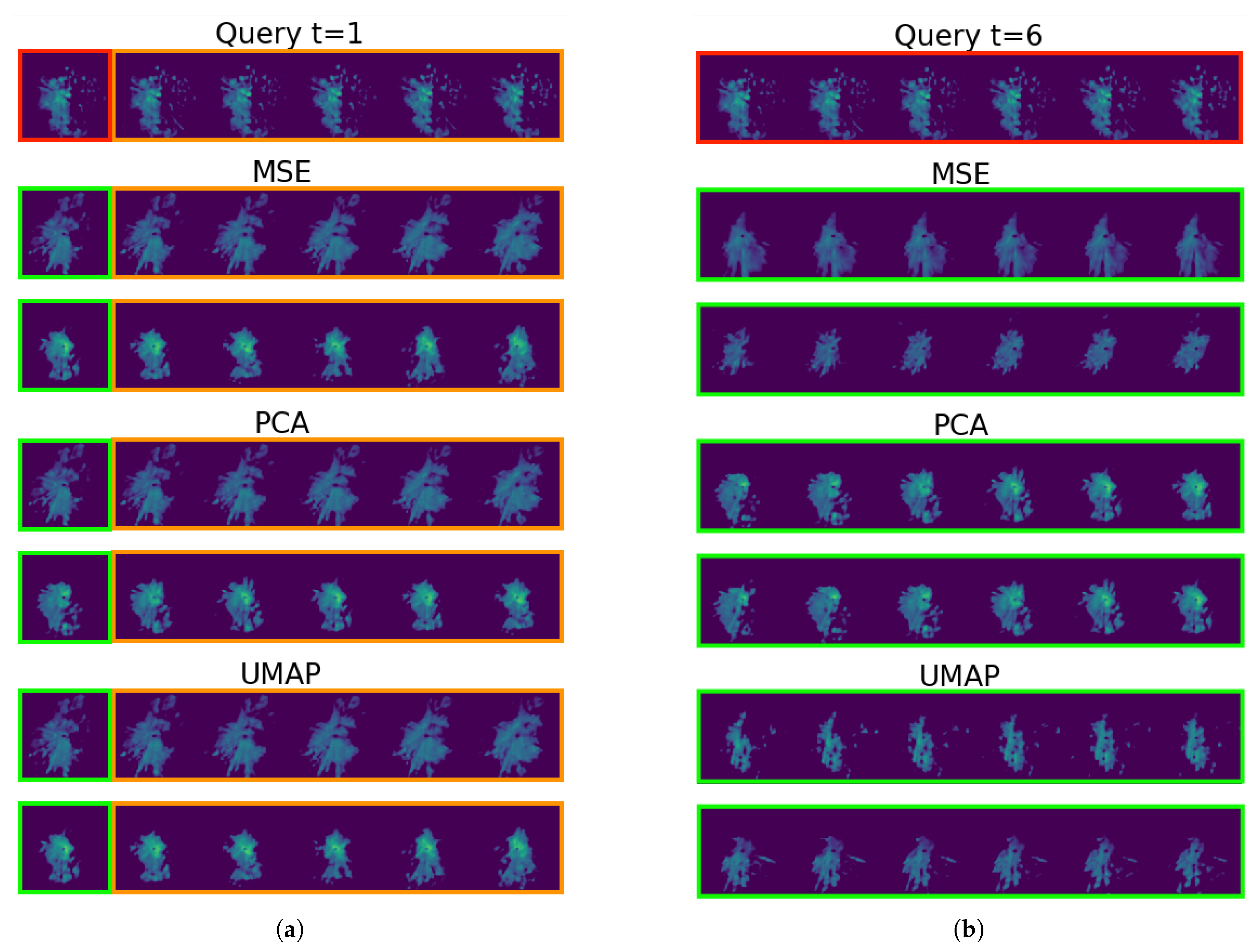
To assess the improvement in analog retrieval, given by using sequence of images instead of extending in time the results from single frame search, we computed, for the 1226 sequences used in Section 3.3, the average MSE score difference between the queries and the top-50 results at and considering the whole sequence or only the first image for the match: we found that using sequences to query reduces the average MSE of the analogs by 4.6% and 10.9% for and respectively. Figure A15 shows an example of this behavior: a longer query helps to better match the evolution of the precipitation patterns.
Figure A15.
Example of a query result for frames when using as input (red box) a single radar scan (a) or the whole sequence (b). The matching sequences are marked in green, while in orange are highlighted the time extensions.
Figure A15.
Example of a query result for frames when using as input (red box) a single radar scan (a) or the whole sequence (b). The matching sequences are marked in green, while in orange are highlighted the time extensions.

References
- Lorenz, E.N. Atmospheric predictability as revealed by naturally occurring analogues. J. Atmos. Sci. 1969, 26, 636–646. [Google Scholar] [CrossRef] [Green Version]
- Delle Monache, L.; Nipen, T.; Liu, Y.; Roux, G.; Stull, R. Kalman filter and analog schemes to postprocess numerical weather predictions. Mon. Weather Rev. 2011, 139, 3554–3570. [Google Scholar] [CrossRef] [Green Version]
- Zorita, E.; Von Storch, H. The analog method as a simple statistical downscaling technique: Comparison with more complicated methods. J. Clim. 1999, 12, 2474–2489. [Google Scholar] [CrossRef]
- Lguensat, R.; Tandeo, P.; Ailliot, P.; Pulido, M.; Fablet, R. The analog data assimilation. Mon. Weather Rev. 2017, 145, 4093–4107. [Google Scholar] [CrossRef] [Green Version]
- Tandeo, P.; Ailliot, P.; Ruiz, J.; Hannart, A.; Chapron, B.; Cuzol, A.; Monbet, V.; Easton, R.; Fablet, R. Combining analog method and ensemble data assimilation: Application to the Lorenz-63 chaotic system. In Machine Learning and Data Mining Approaches to Climate Science; Springer: Berlin, Germany, 2015; pp. 3–12. [Google Scholar]
- Shahriari, M.; Cervone, G.; Clemente-Harding, L.; Monache, L.D. Using the analog ensemble method as a proxy measurement for wind power predictability. Renew. Energy 2020, 146, 789–801. [Google Scholar] [CrossRef]
- Bergen, R.E.; Harnack, R.P. Long-range temperature prediction using a simple analog approach. Mon. Weather Rev. 1982, 110, 1083–1099. [Google Scholar] [CrossRef] [Green Version]
- Delle Monache, L.; Eckel, F.A.; Rife, D.L.; Nagarajan, B.; Searight, K. Probabilistic Weather Prediction with an Analog Ensemble. Mon. Weather Rev. 2013, 141, 3498–3516. [Google Scholar] [CrossRef] [Green Version]
- Alessandrini, S.; Delle Monache, L.; Sperati, S.; Nissen, J. A novel application of an analog ensemble for short-term wind power forecasting. Renew. Energy 2015, 76, 768–781. [Google Scholar] [CrossRef]
- Alessandrini, S.; Delle Monache, L.; Sperati, S.; Cervone, G. An analog ensemble for short-term probabilistic solar power forecast. Appl. Energy 2015, 157, 95–110. [Google Scholar] [CrossRef] [Green Version]
- Van den Dool, H. Searching for analogues, how long must we wait? Tellus A 1994, 46, 314–324. [Google Scholar] [CrossRef]
- Panziera, L.; Germann, U.; Gabella, M.; Mandapaka, P.V. NORA–Nowcasting of Orographic Rainfall by means of Analogues. Q. J. R. Meteorol. Soc. 2011, 137, 2106–2123. [Google Scholar] [CrossRef]
- Sokol, Z.; Mejsnar, J.; Pop, L.; Bližňák, V. Probabilistic precipitation nowcasting based on an extrapolation of radar reflectivity and an ensemble approach. Atmos. Res. 2017, 194, 245–257. [Google Scholar] [CrossRef]
- Atencia, A.; Zawadzki, I. A Comparison of Two Techniques for Generating Nowcasting Ensembles. Part II: Analogs Selection and Comparison of Techniques. Mon. Weather Rev. 2015, 143, 2890–2908. [Google Scholar] [CrossRef]
- Sun, J.; Xue, M.; Wilson, J.W.; Zawadzki, I.; Ballard, S.P.; Onvlee-Hooimeyer, J.; Joe, P.; Barker, D.M.; Li, P.W.; Golding, B.; et al. Use of NWP for nowcasting convective precipitation: Recent progress and challenges. Bull. Am. Meteorol. Soc. 2014, 95, 409–426. [Google Scholar] [CrossRef] [Green Version]
- Foresti, L.; Panziera, L.; Mandapaka, P.V.; Germann, U.; Seed, A. Retrieval of analogue radar images for ensemble nowcasting of orographic rainfall. Meteorol. Appl. 2015, 22, 141–155. [Google Scholar] [CrossRef]
- McInnes, L.; Healy, J.; Saul, N.; Großberger, L. UMAP: Uniform Manifold Approximation and Projection. J. Open Source Softw. 2018, 3, 861. [Google Scholar] [CrossRef]
- Mueen, A.; Zhu, Y.; Yeh, M.; Kamgar, K.; Viswanathan, K.; Gupta, C.; Keogh, E. The Fastest Similarity Search Algorithm for Time Series Subsequences under Euclidean Distance. 2017. Available online: http://www.cs.unm.edu/~mueen/FastestSimilaritySearch.html (accessed on 18 November 2019).
- Jolliffe, I. Principal Component Analysis; Springer: Berlin, Germany, 2011. [Google Scholar]
- Becht, E.; McInnes, L.; Healy, J.; Dutertre, C.A.; Kwok, I.W.H.; Ng, L.G.; Ginhoux, F.; Newell, E.W. Dimensionality reduction for visualizing single-cell data using UMAP. Nature Biotechnology, 3 February 2018. [Google Scholar]
- McInnes, L. How UMAP Works. Available online: https://umap-learn.readthedocs.io/en/latest/how_umap_works.html (accessed on 18 November 2019).
- Yeh, C.C.M.; Zhu, Y.; Ulanova, L.; Begum, N.; Ding, Y.; Dau, A.; Silva, D.; Mueen, A.; Keogh, E. Matrix Profile I: All Pairs Similarity Joins for Time Series: A Unifying View That Includes Motifs, Discords and Shapelets. In Proceedings of the 2016 IEEE 16th International Conference on Data Mining (ICDM), Barcelona, Spain, 12–15 December 2016; pp. 1317–1322. [Google Scholar] [CrossRef]
- Yeh, C.C.M. Towards a Near Universal Time Series Data Mining Tool: Introducing the Matrix Profile. arXiv 2018, arXiv:1811.03064. [Google Scholar]
- Dau, H.A.; Keogh, E. Matrix Profile V: A Generic Technique to Incorporate Domain Knowledge into Motif Discovery. In Proceedings of the 23rd ACM SIGKDD International Conference on Knowledge Discovery and Data Mining, KDD ’17, Halifax, NS, Canada, 13–17 August 2017; ACM: New York, NY, USA, 2017; pp. 125–134. [Google Scholar] [CrossRef]
- Gharghabi, S.; Ding, Y.; Yeh, C.C.M.; Kamgar, K.; Ulanova, L.; Keogh, E. Matrix profile VIII: Domain agnostic online semantic segmentation at superhuman performance levels. In Proceedings of the 2017 IEEE International Conference on Data Mining (ICDM), New Orleans, LA, USA, 18–21 November 2017; pp. 117–126. [Google Scholar]
- Zhu, Y.; Yeh, C.C.M.; Zimmerman, Z.; Kamgar, K.; Keogh, E. Matrix profile XI: SCRIMP++: Time series motif discovery at interactive speeds. In Proceedings of the 2018 IEEE International Conference on Data Mining (ICDM), Singapore, 17–20 November 2018; pp. 837–846. [Google Scholar]
- Yang, D.; Alessandrini, S. An ultra-fast way of searching weather analogs for renewable energy forecasting. Sol. Energy 2019, 185, 255–261. [Google Scholar] [CrossRef]
- Erdin, R.; Frei, C.; Künsch, H.R. Data Transformation and Uncertainty in Geostatistical Combination of Radar and Rain Gauges. J. Hydrometeorol. 2012, 13, 1332–1346. [Google Scholar] [CrossRef]
- Jurman, G.; Merler, S.; Barla, A.; Paoli, S.; Galea, A.; Furlanello, C. Algebraic stability indicators for ranked lists in molecular profiling. Bioinformatics 2008, 24, 258–264. [Google Scholar] [CrossRef]
- Lance, G.; Williams, W. Computer programs for hierarchical polythetic classification (“similarity analysis”). Comput. J. 1966, 9, 60–64. [Google Scholar] [CrossRef]
- Jurman, G.; Riccadonna, S.; Visintainer, R.; Furlanello, C. Canberra distance on ranked lists. In Proceedings of the Advances in Ranking NIPS 2009 Workshop, Vancouver, BC, Canada, 11 December 2009; pp. 22–27. [Google Scholar]
- Jaccard, P. The distribution of the flora in the alpine zone. 1. New Phytol. 1912, 11, 37–50. [Google Scholar] [CrossRef]
- Sampat, M.P.; Wang, Z.; Gupta, S.; Bovik, A.C.; Markey, M.K. Complex wavelet structural similarity: A new image similarity index. IEEE Trans. Image Process. 2009, 18, 2385–2401. [Google Scholar] [CrossRef] [PubMed]
- Von Hardenberg, J.; Ferraris, L.; Provenzale, A. The shape of convective rain cells. Geophys. Res. Lett. 2003, 30. [Google Scholar] [CrossRef]
Figure 1.
Data preprocessing pipeline. The whole dataset is first filtered to remove data chunks that do not contain a interesting amount of signal. A bilinear interpolation filter is applied to the images to reduce the resolution from 480 × 480 to 64 × 64 pixels. The transformed dataset is then split into search and verification sets.

Figure 2.
The MASS-UMAP workflow.

Figure 3.
Workflow of the model development for the UMAP training and verification. The same workflow is used for training and verification of the principal component analysis (PCA), which is used as a comparison method.
Figure 3.
Workflow of the model development for the UMAP training and verification. The same workflow is used for training and verification of the principal component analysis (PCA), which is used as a comparison method.

Figure 4.
UMAP embedding visualization of the second and third components for search space (a) and for verification space (b). The embeddings are colored by wet area ratio (WAR).
Figure 4.
UMAP embedding visualization of the second and third components for search space (a) and for verification space (b). The embeddings are colored by wet area ratio (WAR).

Figure 5.
Canberra stability indicator results for PCA with different values of limit k and components d (darker/lower is better). Lower values indicates that the configuration better preserves the rankings found computing MSE on the original images. The mean, standard deviation, and suboptimal scenario, given by the sum of mean and standard deviation, are reported.

Figure 6.
Jaccard values for PCA with different values of limit k and components d (darker/lower is better). The number in parentheses is the cardinality of the intersections between the top-k PCA list and the top k MSE list. Mean, standard deviation, and the “suboptimal scenario”. given by the sum of mean and standard deviation. are reported.

Figure 7.
Jaccard results for UMAP models trained with neighbors .

Figure 8.
Jaccard results for UMAP models trained with neighbors .

Figure 9.
Jaccard results for UMAP models trained with neighbors .

Figure 10.
Jaccard results for UMAP models trained with neighbors .

Figure 11.
Jaccard results for UMAP models trained with neighbors .

Figure 12.
UMAP Jaccard score for the chosen value of neighbor vs. PCA. Only and are drawn for UMAP, as the values are overlapping for d from 5 to 100. In panel (b), the shade represents the standard deviation.
Figure 12.
UMAP Jaccard score for the chosen value of neighbor vs. PCA. Only and are drawn for UMAP, as the values are overlapping for d from 5 to 100. In panel (b), the shade represents the standard deviation.

Figure 13.
Mean MSE values for analog sequences of obtained with PCA ( and components), UMAP ( components) and MSE search in original space. Dotted lines represent the standard deviation of the MSE.
Figure 13.
Mean MSE values for analog sequences of obtained with PCA ( and components), UMAP ( components) and MSE search in original space. Dotted lines represent the standard deviation of the MSE.

Figure 14.
Mean MSE values for analog sequences of obtained with PCA ( and components), UMAP ( components) and MSE search in original space. Dotted lines represent the standard deviation of the MSE.
Figure 14.
Mean MSE values for analog sequences of obtained with PCA ( and components), UMAP ( components) and MSE search in original space. Dotted lines represent the standard deviation of the MSE.

Figure 15.
Mean MSE values for analog sequences of obtained with PCA ( and components), UMAP ( components) and MSE search in original space. Dotted lines represent the standard deviation of the MSE.
Figure 15.
Mean MSE values for analog sequences of obtained with PCA ( and components), UMAP ( components) and MSE search in original space. Dotted lines represent the standard deviation of the MSE.

Figure 16.
Mean MSE values for analog sequences of obtained with PCA ( and components), UMAP ( components) and MSE search in original space. Dotted lines represent the standard deviation of the MSE.
Figure 16.
Mean MSE values for analog sequences of obtained with PCA ( and components), UMAP ( components) and MSE search in original space. Dotted lines represent the standard deviation of the MSE.

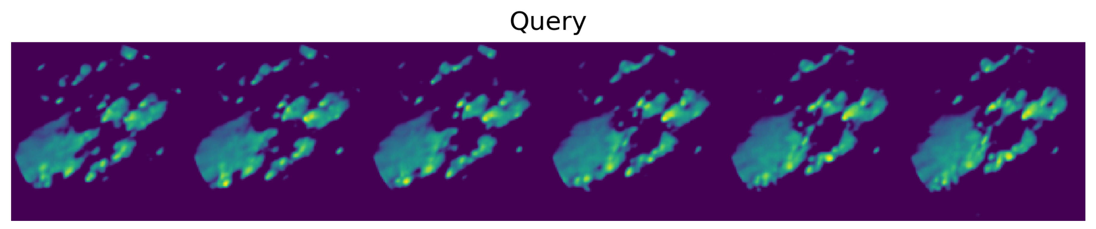
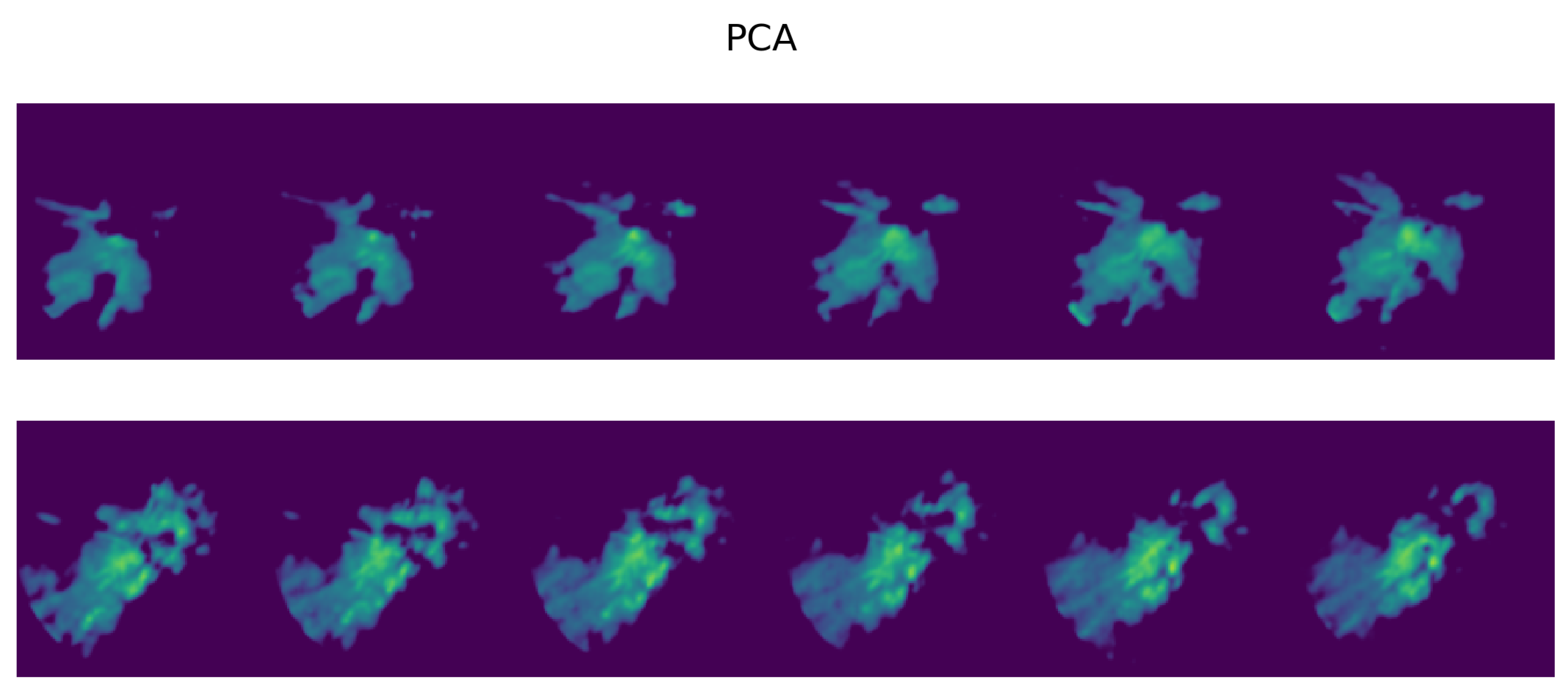
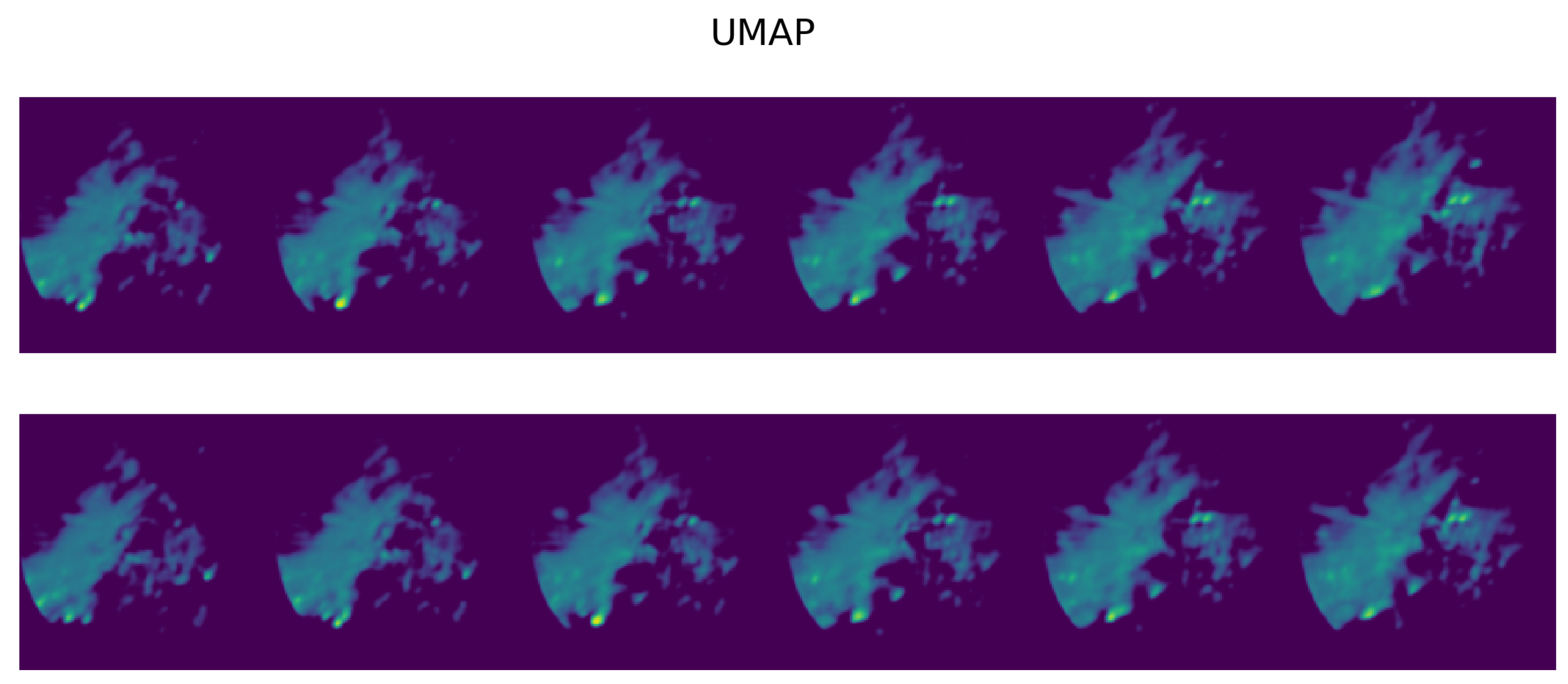
Figure 17.
Sample query sequence of radar scans sampled from the verification set.

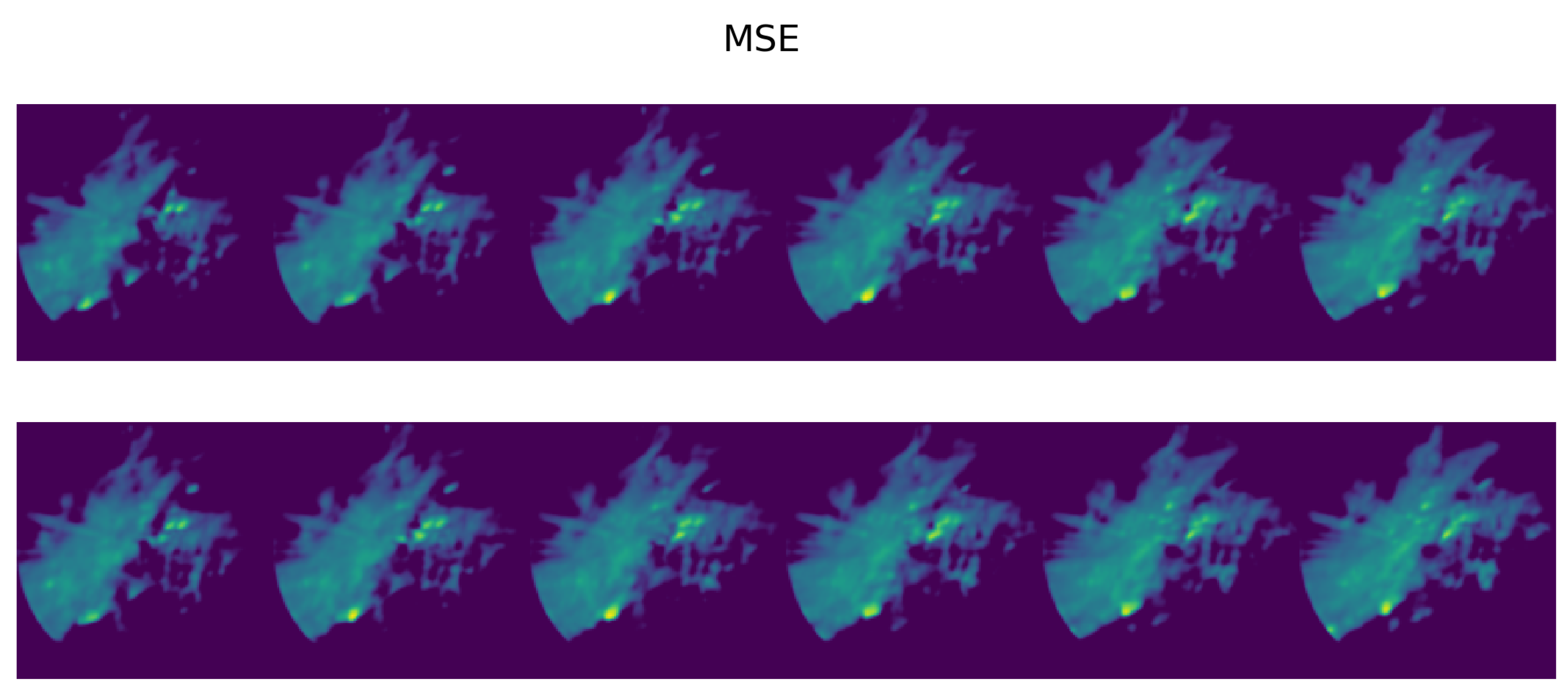
Figure 18.
Top-2 most similar sequences found in training set for the query sequence shown in Figure 17 using MSE comparison on the original radar scans.
Figure 18.
Top-2 most similar sequences found in training set for the query sequence shown in Figure 17 using MSE comparison on the original radar scans.

Figure 19.
As in Figure 18, but searching PCA embeddings () with MASS. PCA embeddings fail to provide any correspondence with the reference sequences found by MSE.
Figure 19.
As in Figure 18, but searching PCA embeddings () with MASS. PCA embeddings fail to provide any correspondence with the reference sequences found by MSE.

Figure 20.
As in Figure 18, but searching UMAP embeddings () with MASS. Although the match is not perfect, UMAP sequences provide at least a partial match with the reference ones in Figure 18.


Table 1.
Table of parameters.
| UMAP training parameter used to define a minimum distance between elements in the low dimensional representation. In our study this value is fixed to . | |
| UMAP training parameter used to compare images in original space. In this study we use the Euclidean distance (the Euclidean distance is rank invariant with respect to the MSE). | |
| n | UMAP training parameter used to define the number of nearest neighbors to build the local distance function. N is the set of all tested values of n. |
| d | Number of components (dimensions) used by the dimensionality reduction (UMAP/PCA). D is the set of all tested values of d. |
| t | Length of the query sequence (number of consecutive radar images) to match. T is the set of all tested values of t. |
| k | Number of closest analogues to consider for further processing. K is the set of all tested values of k. |
| Number of radar images in the search set (archive). The search set contains all the valid data from 2010 to 2016. | |
| Number of radar images in the verification set (query data). The verification set contains all the valid data from 2017 to 2019. |
Table 2.
MASS-UMAP execution times comparison with linear MSE search.
| Sequence Length | 3 | 6 | 12 | 24 |
|---|---|---|---|---|
| (1) UMAP Transform | 194 ms ± 6.72 ms | 303 ms ± 8.87 ms | 451 ms ± 11.3 ms | 745 ms ± 15.5 ms |
| (2) MASS search | 1.01 s ± 9.11 ms | 1.05 s ± 13.4 ms | 1.12 s ± 23.1 ms | 1.31 s ± 25 ms |
| (3) top-k MSE reorder | 11.1 ms ± 0.12 ms | 43.6 ms ± 0.72 ms | 86.4 ms ± 1.27 ms | 172 ms ± 1.11 ms |
| MASS-UMAP (1 + 2 + 3) | 1.22 s ± 15.6 ms | 1.37 s ± 23.0 ms | 1.66 s ± 35.7 ms | 2.23 s ± 35.67 ms |
| MASS-UMAP end-to-end | 1.18 s ± 22.5 ms | 1.37 s ± 48.4 ms | 1.65 s ± 82.9 ms | 2.3 s ± 11.9 ms |
| linear MSE search | 9.59 s ± 1.08 s | 20.4 s ± 1.6 s | 39.5 s ± 3.74 s | 1min 24s ± 1.02 s |
| MASS-UMAP speedup | 8.1× | 14.9× | 23.9× | 36.5× |
© 2019 by the authors. Licensee MDPI, Basel, Switzerland. This article is an open access article distributed under the terms and conditions of the Creative Commons Attribution (CC BY) license (http://creativecommons.org/licenses/by/4.0/).
Share and Cite
MDPI and ACS Style
Franch, G.; Jurman, G.; Coviello, L.; Pendesini, M.; Furlanello, C. MASS-UMAP: Fast and Accurate Analog Ensemble Search in Weather Radar Archives. Remote Sens. 2019, 11, 2922. https://0-doi-org.brum.beds.ac.uk/10.3390/rs11242922
AMA Style
Franch G, Jurman G, Coviello L, Pendesini M, Furlanello C. MASS-UMAP: Fast and Accurate Analog Ensemble Search in Weather Radar Archives. Remote Sensing. 2019; 11(24):2922. https://0-doi-org.brum.beds.ac.uk/10.3390/rs11242922
Chicago/Turabian StyleFranch, Gabriele, Giuseppe Jurman, Luca Coviello, Marta Pendesini, and Cesare Furlanello. 2019. "MASS-UMAP: Fast and Accurate Analog Ensemble Search in Weather Radar Archives" Remote Sensing 11, no. 24: 2922. https://0-doi-org.brum.beds.ac.uk/10.3390/rs11242922
Note that from the first issue of 2016, this journal uses article numbers instead of page numbers. See further details here.