Hyperspectral Anomaly Detection with Harmonic Analysis and Low-Rank Decomposition


1
School of Physics and Optoelectronic Engineering, Xidian University, No. 2, South Taibai Road, Xi’an 710071, China
2
National Institute of Informatics, Tokyo 101-8340, Japan
*
Authors to whom correspondence should be addressed.
Remote Sens. 2019, 11(24), 3028; https://0-doi-org.brum.beds.ac.uk/10.3390/rs11243028
Submission received: 22 October 2019
/
Revised: 5 December 2019
/
Accepted: 13 December 2019
/
Published: 16 December 2019
Abstract
:Hyperspectral anomaly detection methods are often limited by the effects of redundant information and isolated noise. Here, a novel hyperspectral anomaly detection method based on harmonic analysis (HA) and low rank decomposition is proposed. This paper introduces three main innovations: first and foremost, in order to extract low-order harmonic images, a single-pixel-related HA was introduced to reduce dimension and remove redundant information in the original hyperspectral image (HSI). Additionally, adopting the guided filtering (GF) and differential operation, a novel background dictionary construction method was proposed to acquire the initial smoothed images suppressing some isolated noise, while simultaneously constructing a discriminative background dictionary. Last but not least, the original HSI was replaced by the initial smoothed images for a low-rank decomposition via the background dictionary. This operation took advantage of the low-rank attribute of background and the sparse attribute of anomaly. We could finally get the anomaly objectives through the sparse matrix calculated from the low-rank decomposition. The experiments compared the detection performance of the proposed method and seven state-of-the-art methods in a synthetic HSI and two real-world HSIs. Besides qualitative assessment, we also plotted the receiver operating characteristic (ROC) curve of each method and report the respective area under the curve (AUC) for quantitative comparison. Compared with the alternative methods, the experimental results illustrated the superior performance and satisfactory results of the proposed method in terms of visual characteristics, ROC curves and AUC values.
1. Introduction
Hyperspectral image (HSI), which is an image cube that simultaneously acquires spatial information and rich spectral information of the objects, has high spectral resolution (10 nm or less) and a wide spectral coverage (from visible to short-wave infrared) [1]. The recorded spectral reflection characteristics of the objects can fully reflect the inherent nature of the objects [2,3]. Therefore, target detection and recognition can be performed by the spatial-spectral information provided by the HSI [4,5]. According to whether priori information is used, the target detection methods are classified into two categories: supervised and unsupervised [6]. Anomaly detection is an unsupervised method, which is more practical than supervised target detection because it does not require the prior information of the target. Anomaly detection has been widely applied to the fields of maritime search and rescue, geological survey, fire disaster monitoring and battlefield target detection [7].
At present, many anomaly detection methods have been developed. The iconic hyperspectral anomaly detection method is proposed by Reed-Xiaoli (RX) [8,9], and its variant, the local RX (LRX) method [10]. However, its assumptions on the background model are too simple, which limits the detection performance [11]. Moreover, it is difficult to avoid the contamination of the anomaly and noise when calculating the statistical distribution characteristics of the background. As a result, many improved methods have been proposed [12]. For example, the subspace-based RX (SSRX) method [13] made the background statistical characteristic evaluation more robust by a projection transformation of the covariance matrix. The random-selection-based anomaly detector (RSAD) [14] iteratively selected a set of robust background feature pixels in HSI by adopting a random approach. The method could obtain background statistical characteristic evaluation parameters that exclude the interference of anomaly. Due to the fact that anomaly and background are linearly inseparable, Kown et al. [15] suggested that the kernel method was worked to project the traditional RX (KRX) method into the high-dimensional kernel feature space. Then, the anomaly could be separated from the background. Traditional RX-based improved methods typically model the background before performing the complex calculations. Therefore, the performance of such methods was limited due to anomaly and noise contamination that may violate the assumption on background. As a consequence, other types of methods have also been explored.
In recent years, harmonic analysis (HA) [16], which was first proposed by Jakubauskas et al., has attracted broad attention in the image process area. In the field of remote sensing data processing, HA was initially exploited to analyze time series data [17]. A curve fitting method based on HA [18] was proposed to better understand the change of natural land cover. In hyperspectral unmixing, a mixture model based on harmonic combination description was introduced [19]. An HSI classification method called HA-PSO-SVM [20] was proposed by combining HA and particle swarm optimization (PSO) optimized support vector machine (SVM). It is shown that, through the above analysis, harmonic analysis can be used for hyperspectral anomaly detection.
More recently, filtering-based methods have been introduced into anomaly detection. To solve the unreasonable problem of the assumptions of the RX method, whitening spatial correlation filtering (WSCF) [21] was described by Gaucel et al. Anomaly detector based on attribute and edge-preserving filters (AED) [22] was examined by Kang et al. The AED method detected anomalies by introducing local morphological attribute filtering after dimensionality reduction. The domain transform recursive filter as a follow-up operation had been proved to be able to remove the noise and maintain the edges. Multiscale attribute and edge preserving filters-based method [23] was discussed by Li et al. to consider multiscale information in HSI. This method concentrated on the spatial structure information of anomaly targets in HSI. To solve redundant data and noise bands in HSI, structure tensor and guided filtering (STGF)-based anomaly detection method [24] was proposed by combining attribute filtering.
In addition to the above methods, the representation based has gained much attention of researchers. For the first time, Chen et al. [25] introduced sparse representations into the hyperspectral target detection and achieved extraordinary results. This method represented the pixel under test by a few pixels in the neighborhood. After this, Li et al. originally proposed a collaborative representation-based [26] anomaly detection method (CRD). Unlike the sparse representation, the pixels under test were represented by all the pixels in the neighborhood in the collaborative representation. Another type of representation-based approach that has been applied to anomaly detection is based on low-rank decomposition. Xu et al. [27] separated the anomaly from the low rank background through robust principal component analysis (RPCA) [28]. In order to take advantage of neglected low rank background information and reduce false alarm rate, Zhang et al. [29] combined low-rank and sparse decomposition based on Go Decomposition (GoDec) with Mahalanobis distance (LSMAD). The difference between this method and others is that the statistical characteristic of the decomposed low-rank component was added to the Mahalanobis distance detection. Xu et al. first developed an anomaly detection method based on low-rank and sparse representation (LRASR) [30] by combining local and global structure information in HSI. The LRASR method established a background dictionary by k-means clustering. Niu et al. [31] argued that the background dictionary constructed by adding a random selection method to the iterative update of dictionary exhibits more excellent performance in low-rank decomposition. This one made low-rank decomposition more robust by avoiding the contamination of anomaly. To alleviate the effect of noise and mixed pixels, Qu et al. [32] performed abundance and dictionary-based low-rank decomposition (ADLR) to obtain the residual matrix. Thus, anomaly was detected from the residual matrix. The advantage of the ADLR method was that the abundance vector obtained by spectral unmixing, whose low-rank decomposition was more accurate. However, most anomaly detection methods do not take into account the redundant information and isolated noise in HSI.
In this paper, we propose a novel hyperspectral anomaly detection method based on HA and low rank decomposition (HALR) to overcome the above problems. There are three main contributions in the proposed HALR method. Initially, low-order harmonic images of the HSI are extracted by performing HA in a single pixel. The HA can reduce the dimension of HSI and remove the redundant information in HSI. Moreover, in order to reduce the effects of isolated noise and suppress background, the low-order harmonic images are filtered by the guided filtering (GF). Hence, the initial smoothed images that were obtained by the differential operation replace the original HSI to detect anomalies. At the same time, a novel background dictionary construction method is proposed. The extracted background dictionary can fully represent background features. Eventually, anomalies can be obtained by performing dictionary-based low-rank decomposition on the initial smoothed images. The low-rank decomposition takes full advantage of the fact that the background is low-rank and the anomaly is sparse. The experimental results verify the superiority of the proposed HALR method in terms of detection performance.
The rest of this paper is organized as follows. The second part describes the proposed HALR method. The third part illustrates the experimental results. The fourth part is the parameter setting discussion. The fifth draws the conclusions.
2. Harmonic Analysis and Low-Rank Decomposition
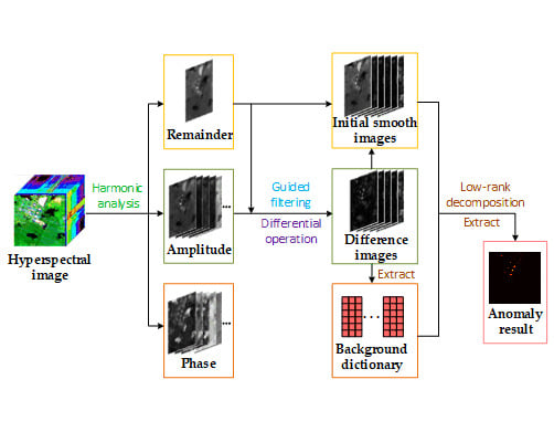
The flowchart of the proposed HALR-based method is shown in Figure 1. The proposed HALR method mainly includes three strategies. In the beginning, low-order harmonic images are obtained by HA. Then, the initial smooth images are gained by GF and differential operation. At the same time, a background dictionary is obtained through a new background dictionary construction method. Finally, anomaly can be acquired by the low-rank decomposition.
2.1. Hyperspectral Harmonic Analysis
HSI has a lot of redundant information because of the high correlation of adjacent bands. Due to the influence of noise and the atmosphere, not all bands can provide valid information [33]. Because of this, the hyperspectral data are regarded as the timing signal from the perspective of time domain signals. Then, HA is introduced to perform time-frequency space conversion on the timing signal. The theory of HA is to represent any time-series function f(t) with respect to time t by superposition of sine or cosine waves (harmonics) [34].
Different from the traditional Fourier transform [35] than from the spatial domain to the frequency domain, HA utilizes spectral information and correlation between bands in the HSI to transform from time domain to spatial domain. By making full use of the hyperspectral spectral characteristics, the hyperspectral data is transformed into a set of components that is composed of energy spectral characteristic components by the harmonic analysis, while the spatial characteristics of the hyperspectral data remain unchanged. Specifically for a single pixel, multiple harmonic analysis can express the spectral information of each pixel as the sum of the superposition of the sine waves (cosine waves), which is composed of a series of harmonic energy characteristic parameter components. In this way, the spectrum of each pixel can be represented as a complex, continuous and smooth curve.
When HA is employed to process spectral data, the approximately continuous spectral curve composed of B bands can be treated as a function of period B. After harmonic decomposition, the spectral curve of each pixel in the HSI can be expressed as the sum of the superposition of the sine waves (cosine waves) composed of a series of harmonic energy characteristic parameter components, including harmonic remainder, amplitude and phase [20]. If it is known that the spectral vector consisting of B bands can be represented as Yi = [y1, y2, …, yn, …, yB]T, the spectral value of each band is recorded as yn, where n is the band serial number (n = 1, 2, …, B). Therefore, the harmonic decomposition expansion of the h-th harmonic analysis of the spectral vector Yi is:
The harmonic energy characteristic parameter components of the h-th harmonic decomposition of Yi are calculated as:
where h (h = 1, 2, 3, …) is the number of harmonic decompositions; Re is the remainder of the harmonic; is the h-th harmonic component; Ch, Sh, Hh and Ph are the cosine amplitude, sine amplitude, harmonic component amplitude and harmonic component phase of the h-th harmonic decomposition, respectively. Here, the remainder represents the average of the spectral, the amplitude and phase respectively reflect energy changes in different bands and the position of the band where the amplitude of the energy appears [36]. The detailed steps of hyperspectral HA are described in Algorithm 1.
In the HA, the lower harmonics contain the main energy characteristics of the spectral and the higher harmonics are usually mixed with noise information. Therefore, harmonic analysis has better noise cancellation and main energy extraction capabilities, and it can also preserve the spatial feature information of hyperspectral data.
Since the low-order harmonics contain most of the energy of the HSI, not all harmonic images can provide crucial information. As such, we can select the first few low-order harmonic images as the subsequent test images. However, not all images in low-order harmonic images are suitable for anomaly detection. As shown in Figure 2, it can be clearly seen that the phase in low-order harmonic images contains a lot of interference and useless information. Thus, the phase in low-order harmonic images is directly discarded. The remainder and amplitude are preserved. Finally, the remainder and the first five amplitude images are adopted for subsequent test images. In this way, the ultimate goal of hyperspectral HA in this part is to reduce dimensionality and remove redundant information.
| Algorithm 1. Harmonic analysis |
| 1. Input: Hyperspectral matrix Y = [Y1, Y2, …, YM] ∈ RB×M, maximum harmonic number hmax. |
| 2. Transformation process |
| for each pixel Yi do |
| (1) calculate remainder Re by Equation (2); |
| for h = 1 to hmax do |
| (2) Calculate coefficients of HA by Equations (3)–(6); |
| end for |
| (3) Get the reconstructed pixel Y′i by Equayion (1); |
| end for |
| 3. Output: remainder Re, amplitude Hh and phase Ph. |
2.2. Guided Filtering and Dictionary Construction
Although HA achieves dimensionality reduction and removes redundant information in the HSI, the resulting image still retains some isolated noise. Next, GF and differential operation is applied to further reduce the isolated noise and enhance the detail in the image [37,38]. In addition, it should be mentioned that the GF can also smooth the background to a certain extent.
2.2.1. Guided Filtering
In GF, it is crucial to choose the guidance image sensibly [39]. The guidance image directly affects the result of the filtered output. In this part, the remainder Re is taken as the guide image. The five amplitude images Hj (j = 1, 2, …,5) are recorded as input images, and Gj are recorded as output images. The GF output images Gj can be obtained as follows:
where Wk represents a window of (2r + 1) × (2r + 1); k is the center of the window Wk; x is the pixel index in window Wk; ak and bk are the fixed coefficients of the linear function in the window Wk, respectively.
In order to minimize the difference between the output image and the input image, the minimum cost function expression is as follows:
where ε is the regularization coefficient. The expressions for ak and bk are as follows:
where uk and δk are the mean and variance of the image Re in the window Wk; |w| is the total number of elements in the window Wk; Vk is the mean of the image Hj in the window Wk, respectively.
Some examples of GF are illustrated in Figure 3. Figure 3a shows the remainder Re as a guide image. Figure 3b,d show the first-order amplitude image H1 and H2 as GF input images, respectively. Figure 3c,e denote the output images G1 and G2 of Figure 3b,d, respectively. It can be seen from Figure 3 that the background is smoothed by the GF.
After getting the output images Gj of the GF, differential operation is introduced to calculate the difference between the input images Hj and the output images Gj:
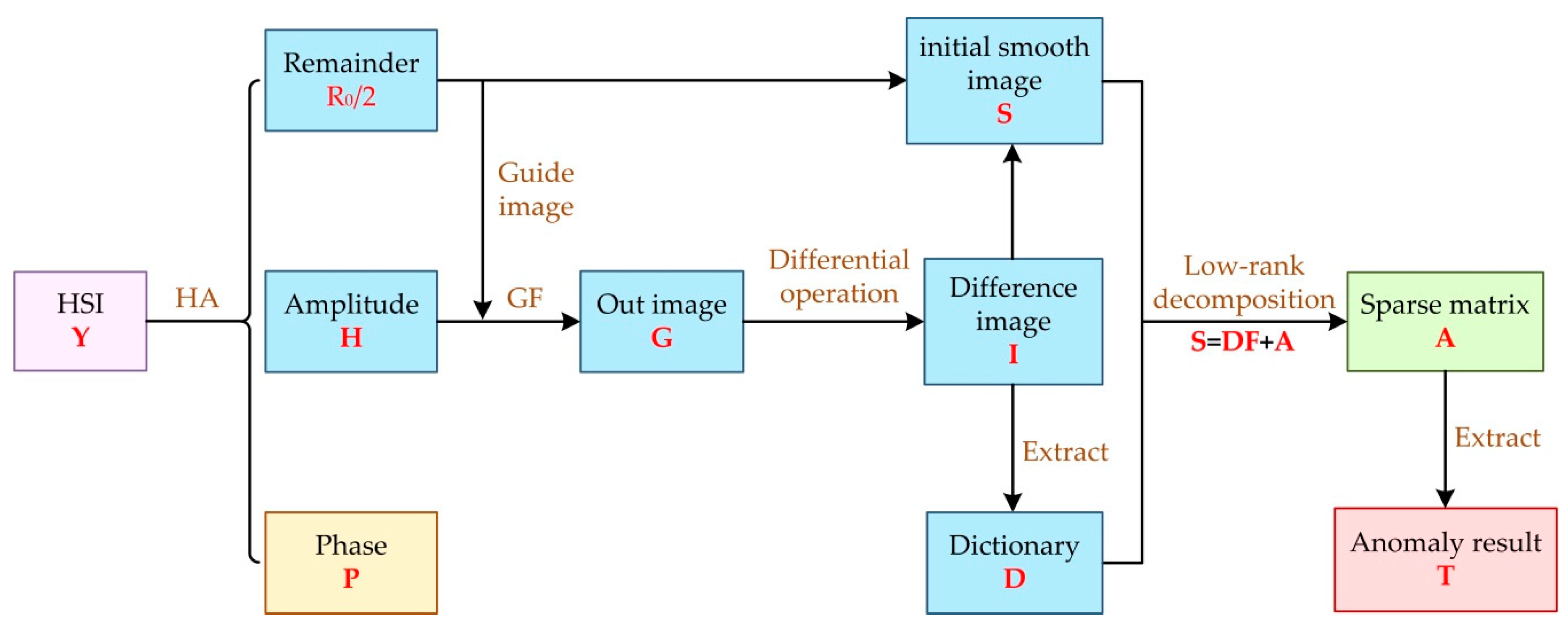
where Ij is the difference image. This differential operation can alleviate the isolated noise [40,41] in the input image to a certain extent. Although anomalies are also suppressed after GF and differential operations, background and isolated noise are simultaneously suppressed. It can highlight anomaly and enhance the detail while suppressing the background. A wealth of information with respect to anomaly is to be found in the difference image. Figure 4 is shown as an example, where Figure 4a,d are difference images I1 and I2, respectively.
In order to make use of distinctive characteristics of differential images in detecting anomalies, the harmonic remainder Re and the difference image Ij replaces the original HSI as initial smooth images S Rl×M for low rank decomposition. l indicates that each pixel in the initial smooth images S is an l-dimensional column vector.
Figure 5 reveals an example of the formation of the initial smooth images S. The initial smooth images S can be obtained by transforming the three-dimensional cube composed of the harmonic remainder Re and the difference image Ij into a two-dimensional matrix.
2.2.2. Dictionary Construction
In the low-rank decomposition, the background dictionary is of great importance. A satisfactory background dictionary usually contains various background categories in the image under test, while eliminating interference from anomaly and noise [42,43]. In this section, a rational method is studied instead of directly using original HSI or dictionary learning method to establish a background dictionary.
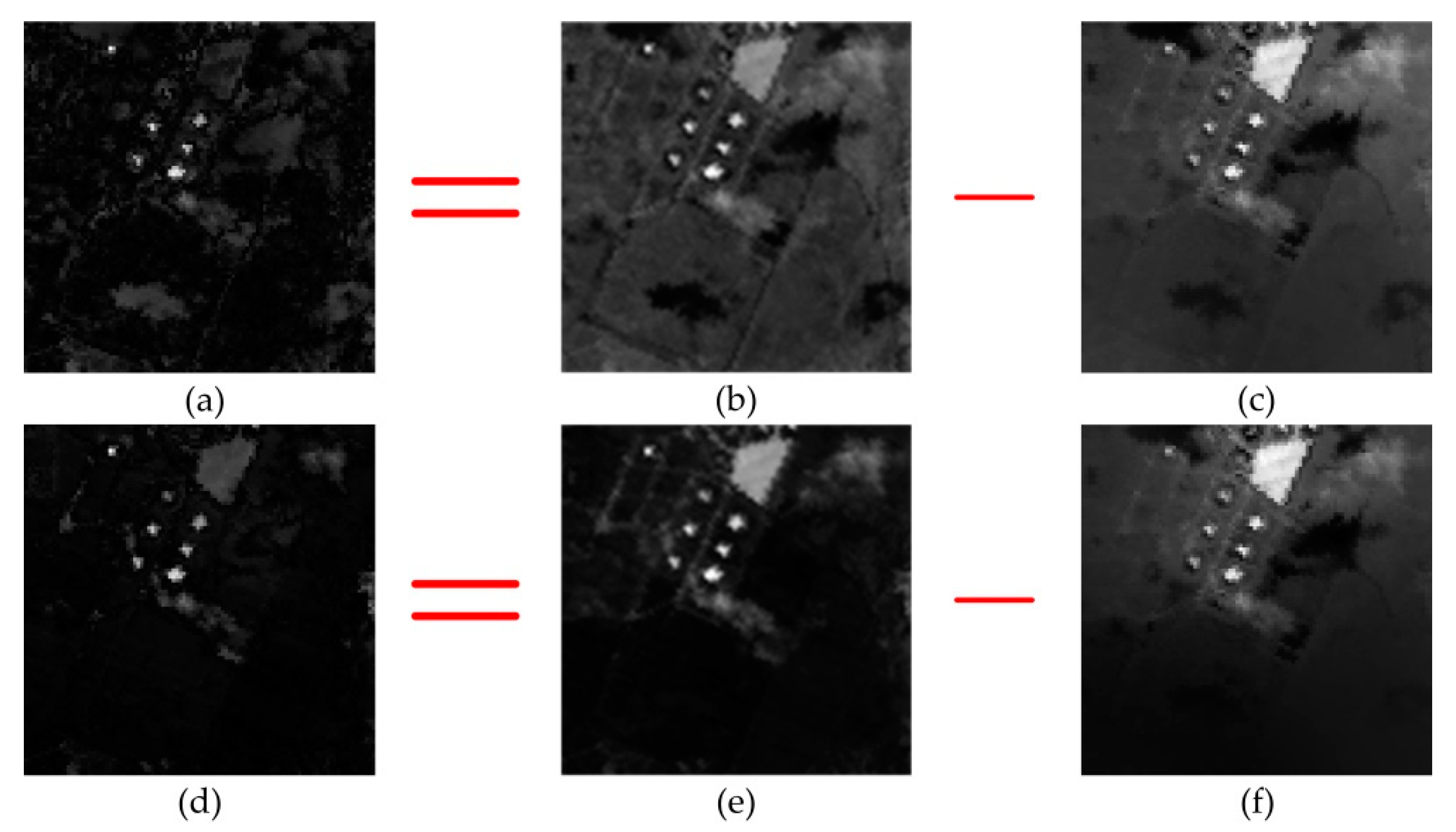
In order to extract a suitable background dictionary from the initial smooth images S, the difference image I is first fused. To further reduce the interference of anomalies and noise on the background dictionary, pixels in the fused image are sorted in ascending order and segmented. Then, for the sorted pixels after segmentation, the part with a large pixel value is considered to be an anomaly and noise pixel set, and the part with a small pixel value is considered to be a background pixel set. Finally, in order to ensure that the background dictionary atoms contain as many different background categories as possible, we randomly select some pixels from the background pixel set as representative and discriminative background dictionary atoms. The extracted background dictionary is applied for subsequent low-rank decomposition.
We take the column vectors of the initial smooth images S as samples. Firstly, the resulting difference images are merged together. The fusion method is denoted as:
where d is the merged image, which will be used as the basis for dictionary extraction.
After merging, anomaly pixels and edges in the image will be highlighted. Consequently, these highlighted points in the image will be numerically larger than background values. After that, the pixels in the fused image d are sorted in ascending order. For sorted pixels, the background pixels will be more forward.
Finally, a part of the pixels φ is randomly selected from the first ξ of the sorted pixels to build background dictionary, where φ is dictionary atom selection percentage and ξ is separated value. Both φ and ξ are percentages. Among them, the value of φ is not fixed, and the value of ξ is 90%. The number of the selected pixels and the value of ξ will be analyzed later. The main objective of random selection is to choose as many categories of background pixels as possible. An example of the background dictionary constructed is displayed in Figure 6.
Through this method, a representative background dictionary DRl×m is obtained, where m represents the total number of atoms in the background dictionary D.
2.3. Low-Rank Decomposition
Since the anomaly is sparse and the background is low-rank in hyperspectral data, the low-rank decomposition in the field of visible light image processing is also applicable to HSI [44,45,46]. However, most of these methods directly implement low-rank decomposition on the original HSI without considering the redundant information of HSI, the correlation between bands and the isolated noise. In this respect, we proposed a novel low-rank decomposition strategy. Here, instead of the original HSI, we performed the low-rank decomposition on the initial smooth images S, which is identified as the object of low-rank decomposition. Then, the decomposition formula is represented as follows:
where FRm×M is a m × M coefficient matrix of all pixels in S; ARl×M is a l × M sparse matrix, respectively. Here, m represents the total number of atoms in the background dictionary D, M represents the total number of pixels in the HIS, and l indicates that each pixel in the initial smooth images S is a l-dimensional column vector.
For the low-rank decomposition problem, there are several solutions. RPCA [28] could decompose the hyperspectral data into the low rank part and the sparse residual part. However, RPCA does not consider the noise of hyperspectral data making the detection results prone to false alarms. The GoDec method [47,48] divides the hyperspectral data into low rank matrix, sparse matrix and noise matrix, taking into account the noise. The LRASR method [30] solves the low rank representation (LRR) [49] problem with low rank and sparse regularization constraints by the linearized alternating direction method with adaptive penalty (LADMAP) [50]. This method implants the l21 regularization constraint to make the majority of the columns in matrix F equal to 0. However, due to the characteristic difference of anomaly in practice, there are some non-zero values in the column of the sparse matrix A. Therefore, the ADLR method [32] replaces the l21 regularization constraint with the l1 regularization constraint. In addition, this l1 regularization constraint can further reduce the impact of isolated noise on anomaly detection. Since the isolated noise has no sparse attributes in the image, they will be clustered into a group because of their similar coefficients. The l21 regularization is the l21 norm of a matrix, which is defined as the sum of the l2 norm of each column in the matrix. The l1 regularization is the l1 norm of a matrix, which is defined as the sum of the absolute values of all the elements of the matrix.
Through the above analysis and comparison, we exploited the ADLR method with the l1 regularization constraint for the low-rank decomposition. In the low-rank decomposition, the coefficient matrix F is low-rank and the sparse matrix A is sparse. After introducing the l1 regularization constraint, the objective function is as follows:
where rank(·) represents the rank function; λ > 0 is the tradeoff parameter used to adjust the low rank part and the sparse part; ||·||1 is the l1 norm, respectively. The abbreviation s.t. refers to “subject to”, which indicating that the constraint is S = DF + A. ||A||1 is specifically expressed as:
where l indicates that each pixel in the initial smooth images S is a l-dimensional column vector, M represents the total number of pixels in the HIS and is the absolute value of the element in the row-th row and col-th column of the matrix A.
To solve the objective function, the rank function is replaced by the matrix nuclear norm ||·||* [51]. Therefore, the objective function can be optimized to:
In order to decouple the objective function (15), an auxiliary variable U is introduced instead of F [52]. The Lagrange equation of the objective function is;
where tr[·] represents the trace of matrix, which is the sum of the diagonal elements of matrix; L1 and L2 are Lagrange multipliers; τ > 0 is the penalty parameter; ||·||F is the F norm, respectively. Since Equation (16) contains multiple variables, it can be solved by alternate iterative update methods. When solving one of the variables, keep the other variables unchanged. Accordingly, the solution process can be broken down into the following form.
(1) Update U when keeping F and A unchanged, the objective function can be reformulated as:
where arg is the abbreviation of argument. The arg min refers to the value of the variable U when the equation behind it reaches the minimum value.
(2) Update F when keeping U and A unchanged, the objective function can be reformulated as:
(3) Update A when keeping F and U unchanged, the objective function can be reformulated as:
Equations (17) and (19) can be optimized by utilizing the singular value thresholding operator [53] and Lemma 1 in literature [54], respectively. In the iterative process, the Lagrange multipliers update formulas are as follows:
The iterative convergence condition is expressed as:
where η is the decomposition error; ||·||∞ is the infinite norm. After the sparse matrix A is obtained by low-rank decomposition, we get the anomaly by the l2 norm. The l2 norm is the square root of the sum of the squares of all the elements in each column of pixels in the matrix. The specific equation is as follows:
where T(i) represents the anomaly detection result of the i-th pixel. A:,i represents the i-th column of pixels in the matrix A, and M represents the total number of pixels in the HSI.
The complete steps of the low-rank decomposition are presented in Algorithm 2.
| Algorithm 2. Low-rank Decomposition |
| Input: Initial smooth image S, background dictionary D. |
| Initialization: Give λ according to different input data, τ = 10−6, η = 10−6, τmax = 1010, ζ = 1.1, F = U = A = L1 = L2 = 0. |
| while not satisfy the convergence condition (21) do |
| (1) Update variable U according to Equation (17); |
| (2) Update variable F according to Equation (18); |
| (3) Update variable A according to Equation (19); |
| (4) Update Lagrange multipliers L1 and L2 according to Equation (20); |
| (5) Update variable τ, where τ = min(τmax, τ*ζ); |
| end while |
| Return: Coefficient matrix F, sparse matrix A. |
| Calculate anomaly result T according to Equation (22); |
| Output: Anomaly result T. |
3. Experimental Results
To verify the validity of the proposed HALR method, the following methods, including the RX method [8], LRX method [10], WSCF method [21], LSMAD method [29], CRD method [26], RPCA-RX method [55] and AED method [22], are selected for comparison. In order to evaluate the detection results quantitatively, the receiver operating characteristic (ROC) and the area under the curve (AUC) are adopted [56]. The ROC curve shows the corresponding relationship between the false alarm rate and the probability of detection under each threshold segmentation result. The AUC value is obtained by calculating the area under the ROC curve of anomaly detector. At the same false alarm rate, the larger the value of AUC is, the better the performance of the detector. In addition, we select the optimal parameters of the alternative methods from original author in term of AUC value or the parameters. Since the background dictionary is randomly chosen, we repeated it 10 times for each experiment and reported the averaged result. Moreover, in order to verify the stability of the proposed HALR method, we also provided the standard deviation of the results of 10 experiments.
3.1. Data Sets
Synthetic Data Set: the synthetic data is generated by a real-world HSI Salinas [44]. This Salinas scene is acquired by the Airborne Visible/Infrared Imaging Spectrometer (AVIRIS). Some parameters of this HSI are shown in Table 1. As shown in Figure 7a, a 150 × 150 size area is selected from the original image of 512 × 217 size as the background of the synthetic data. 204 bands (1–107, 113–153, 168–223) were retained after removing water absorption bands and low signal-to-noise ratio (SNR) bands in the experiment. In the synthetic data, the anomaly target is embedded by the target implantation method [57]. Anomaly Xea is specifically embedded as follows:
where Jbg represents the spectral of the background pixel at the implantation location; Xia indicates the spectral of the implanted anomaly; p is the percentage coefficient of the anomaly. In the synthetic data, the embedded anomaly spectral is also extracted from the Salinas scene. As shown in Figure 7b, six rows and three columns of targets with different size have been embedded obliquely. From left to right, the corresponding p values for each column are 0.6, 0.8 and 1, respectively. The ground truth map of the synthetic data is shown in Figure 7c. The ground truth is labeled with the help of the Environment for Visualizing Images (ENVI) software.
San Diego Data Set: one of the real-world test image in the experiment is a 100 × 100 image cropped from the original 400 × 400 San Diego HSI [46]. The HSI has a spectral range from 0.37 um to 2.51 um. 189 bands (7–32, 36–96, 98–106, 114–152, 167–220) were retained after removing water absorption bands and low SNR bands in the experiment. Other parameters about the San Diego data set are illustrated in Table 1. Three aircraft in the scene are considered to be anomaly targets to detect. The image under test and the corresponding ground truth map are shown in Figure 8. The ground truth is labeled with the help of the ENVI software.
Beach Data Set: this HSI [22,24] was taken by Reflective Optics System Imaging Spectrometer (ROSIS) sensor. Its wavelength ranges from 0.43 um to 0.86 um. Additional information about this data set is displayed in Table 1. In the experiment, a 100 × 100 area is chosen for the experiment. As shown in Figure 9, the background in the scene is mainly water and bridge. The vehicles on the bridge are considered to be anomaly targets. The ground truth is labeled with the help of the ENVI software.
3.2. Detection Performance Analysis
For the synthetic HSI, the visual detection results of different anomaly detection methods are displayed in Figure 10. It is obvious that the RX method, the WSCF method, the RPCA-RX method and the LSMAD method have poor detection performance in visual effect. We could see in Figure 10 that the RX method, the WSCF method, the RPCA-RX method and the LSMAD method have failed to separate the anomaly from background. Moreover, there are many false alarms in the results of the RPCA-RX method. The visual effect of the AED and CRD detection results are roughly close to the proposed HALR method. However, the false alarm of the proposed HALR method and the CRD method are slightly less than the AED method. The background suppression effect of the CRD method is also similar to that of the AED method and the HALR method. In terms of the ROC curves in Figure 11, the proposed HALR method is still excellent. The AUC values of the respective methods are reported in Table 2. The AUC values of the CRD method and the HALR method both reach a maximum value of 0.9998. The AUC value of the AED method reaches 0.9997, which is substantially equal to the AUC value of the HALR method. From the AUC values in Table 2, the RX method has the worst detection effect. Combined with visual detection results, ROC curves and AUC values, our proposed HALR method is a significant and effective method.
For the San Diego HSI, the false color maps of the detection results of different methods are illustrated in Figure 12. The LRX method has the worst detection result in Figure 12. The size of the aircraft is one of the main reasons that affect the detection result of the LRX method. The RX, WSCF, CRD and RPCA-RX method are not very effective in suppressing background. In consequence, there are numerous false targets in their detection results. The detection results of the proposed HALR method has clearer outline and fewer false alarms than the LSMAD method and the AED method. In Figure 13 shows that the ROC curves of the RX method, the WSCF method, the CRD method, the RPCA-RX method the LSMAD method and the AED method are almost same, while the performance of the HALR method is more remarkable. Above all, the ROC curve of the proposed HALR method is mostly higher than the other curves. Moreover, Table 2 indicates that the AUC value of the proposed HALR method, 0.9939, is the largest. In brief, the proposed HALR method achieved exceptional performance.
For the Beach HSI, the false color maps of the detection results of different methods are illustrated in Figure 14. In terms of visual effects, the CRD method yields the worst detection result. The AED method and the WSCF method do not separate the anomaly targets from the background very well. The detection results of the LSMAD method and the RPCA-RX method are stable, but some false alarms also exist for the RPCA-RX method. The detection results of the RX method, the LRX method and the LSMAD method are similar. Compared to them, the proposed HALR method not only effectively detects the vehicle, but also successfully suppresses the bridge and other backgrounds. We could see that the separation of background and anomaly in the detection result of the proposed HALR method are successful. It is obvious from the ROC curves in Figure 15 that the performance of the AED method is the worst. The ROC curve of the proposed HALR method is lower than the curves of the WSCF method and the RPCA-RX method in a small region. However, under the same false alarm rate, the detection probability of the proposed HALR method reaches 1 the first. Additionally, the curves show that the proposed HALR method has a higher detection probability at a lower false alarm rate than other methods. The AUC values of different methods are presented in Table 2. The AUC value of the proposed HALR method is 0.9920, the largest among all. In summary, the performance of the proposed HALR method is very outstanding.
We reintroduced the standard deviation to further evaluate the effectiveness and stability of the proposed HALR method. In another set of experiment, the AUC value is still the average of the 10 results. At the same time, the standard deviation is calculated. Table 1 shows the 10 AUC values, average AUC values, and standard deviations of the proposed HALR method on three datasets. In the original paper, the average values of AUC on the three datasets were 0.9998, 0.9939 and 0.9920, respectively. As shown in Table 3, the average AUC of the 10 results in another experiment were 0.9998, 0.9926 and 0.9922, respectively. They are very close to the results in the first set of experiments. In addition, the standard deviations of the 10 results on each dataset are 0.00011, 0.0043 and 0.002, respectively. It can be seen from the standard deviations that the performance of our proposed HALR method is still relatively stable.
4. Discussion
The proposed HALR method contains a total of four sensitive parameters. They are the window radius r and the regularization coefficient ε in GF, dictionary atom selection percentage φ, and the tradeoff parameter λ in low-rank decomposition, respectively. The AUC value will be utilized to distinguish the influence of each sensitive parameter on the performance of the HALR method. When analyzing one parameter, the others are fixed as default parameters. As has been noted, the atoms in the background dictionary are selected randomly. Hence, to eliminate the effects of random dictionary, we repeated the test for each value 10 times to report the average score.
For the synthetic hyperspectral dataset, the default parameters are r = 60, ε = 1, φ = 0.001 and λ = 6 × 10⁻⁴, respectively. For the San Diego dataset, the default parameters are r = 20, ε = 0.12, φ = 0.002 and λ = 3 × 10⁻³, respectively. For the Beach dataset, the default parameters are r = 2, ε = 0.32, φ = 0.001 and λ = 1 × 10⁻¹, respectively. The default parameters were selected in order to make the HALR method to achieve optimal performance on the corresponding dataset.
The influence of each sensitive parameter on the AUC performance of the HALR method is demonstrated in Figure 16. When the window radius r parameter is analyzed, due to the different image sizes, the parameter r shows values of only up to 40 in the San Diego HSI and the Beach HSI. For the tradeoff parameter λ, when the parameter λ is greater than or equal to 0.01 while other parameters are fixed, the iterative process of the low-rank decomposition does not converge in the Synthetic HSI and the San Diego HSI. Though there is some variance due to randomness in selecting the atoms in the background dictionary, in general, it can be verified from Figure 16 that the HALR method achieves optimal detection performance under the default parameter settings.
For the parameter hmax, it determines the number of harmonic analysis. In the hyperspectral harmonic analysis, the parameter hmax determines the number of lower harmonics that we should choose. When analyzing the parameter hmax, the other parameters are fixed, the AUC value is used as the evaluation standard. Figure 17 shows the impact of the parameter hmax on the detection results. It can be seen that, for the synthetic dataset, when the parameter hmax is equal to 3 or 5, the detection performance of the proposed HALR method is optimal. For the San Diego and Beach datasets, when the parameter hmax is equal to 3 or 7, respectively, the AUC value of the proposed HALR method reaches the maximum. However, they are slightly larger than the AUC values when the parameter hmax is equal to 5. In order to unify the parameters, the parameter hmax is set as 5. Hence, we finally select the first 5 amplitude images of lower harmonics in the experiment.
Finally, the effect of the separated value ξ on the performance of the proposed HALR method is analyzed. As shown in Figure 18, when the separated value ξ is 90%, the proposed HALR method has the highest performance on all three data sets.
In the experiment, these uncertain parameters are empirically selected which limits the application of the proposed HALR method to some extent. In the future, we will work on the adaptive determination of the various parameters of the proposed HALR method.
5. Conclusions
In this paper, we proposed a novel hyperspectral anomaly detection based on harmonic analysis (HA) and low-rank decomposition. The proposed approach mainly comprises three stages, i.e., HA, guided filter (GF) and low-rank decomposition. In order to deal with large data and redundant information in the original hyperspectral image (HSI), we applied a single-pixel-based HA. Subsequently, we introduced GF on the images after HA, not only to reduce the impact of isolated noise to some extent, but also to make the dictionary more discriminative on the low-rank decomposition. Ultimately, the low-rank decomposition was adopted to extract anomaly objects. The primary goal of this low-rank decomposition was to consider the low-rank features of background and the sparse features of anomaly. Furthermore, both the visual and the quantitative results (receiver operating characteristic (ROC) curves and area under the curve (AUC)) indicate that the proposed approach achieves a more competitive detection performance than alternatives. In the future, we will work on the automatic determination of the optimal parameter.
Author Contributions
Conceptualization, P.X.; methodology, P.X. and H.L.; software, P.X. and J.S.; validation, J.S., H.L. and L.G.; investigation, P.X. and H.L.; resources, P.X.; data curation, L.G.; writing—original draft preparation, P.X., J.S. and H.L.; writing—review and editing, L.G. and H.Z.; visualization, P.X.; supervision, H.Z.; funding acquisition, J.S., H.L. and H.Z.
Funding
This research was funded by the Fundamental Research Funds for the Central Universities under grant number XJS17106 and JB180502, the National Natural Science Foundation of China under grant number 51801142, the Natural Science Foundation of Shaanxi Province under grant number 2018JQ5022.
Conflicts of Interest
The authors declare no conflict of interest.
Abbreviations
| ADLR | Abundance and dictionary-based low-rank decomposition |
| AED | Anomaly detector based on attribute and edge-preserving filters |
| AUC | Area under the curve |
| AVIRIS | Airborne Visible/Infrared Imaging Spectrometer |
| CRD | Collaborative representation-based anomaly detection |
| ENVI | Environment for Visualizing Images |
| GF | Guided filter |
| GoDec | Go Decomposition |
| HA | Harmonic analysis |
| HALR | Harmonic analysis and low-rank decomposition |
| HA-PSO-SVM | Harmonic analysis-particle swarm optimization-support vector machine |
| KRX | Kernel RX |
| LADMAP | Linearized alternating direction method with adaptive penalty |
| LRASR | Low-rank and sparse representation |
| LRR | Low rank representation |
| LRX | Local RX |
| LSMAD | Low-rank and sparse matrix decomposition-based mahalanobis distance method for hyperspectral anomaly detection |
| PSO | Particle swarm optimization |
| ROC | Receiver operating characteristic |
| ROSIS | Reflective Optics System Imaging Spectrometer-03 |
| RPCA | Robust principal component analysis |
| RSAD | Random-selection-based anomaly detector |
| RX | Reed-Xiaoli |
| SNR | Signal-to-noise ratio |
| SSRX | Subspace-based RX |
| STGF | Structure tensor and guided filtering |
| SVM | Support vector machine |
| WSCF | Whitening spatial correlation filtering |
References
- Bioucas-Dias, J.M.; Plaza, A.; Camps-Valls, G.; Scheunders, P.; Nasrabadi, N.; Chanussot, J. Hyperspectral remote sensing data analysis and future challenges. IEEE Geosci. Remote Sens. Mag. 2013, 1, 6–36. [Google Scholar] [CrossRef] [Green Version]
- Ma, D.; Yuan, Y.; Wang, Q. Hyperspectral anomaly detection via discriminative feature learning with multiple-dictionary sparse representation. Remote Sens. 2018, 10, 745. [Google Scholar] [CrossRef] [Green Version]
- Zhu, L.; Wen, G.; Qiu, S. Low-rank and sparse matrix decomposition with cluster weighting for hyperspectral anomaly detection. Remote Sens. 2018, 10, 707. [Google Scholar] [CrossRef] [Green Version]
- Matteoli, S.; Diani, M.; Corsini, G. A tutorial overview of anomaly detection in hyperspectral images. IEEE Aerosp. Electron. Syst. Mag. 2010, 25, 5–28. [Google Scholar] [CrossRef]
- Chang, C.; Chang, S.S. Anomaly detection and classification for hyperspectral imagery. IEEE Trans. Geosci. Remote Sens. 2002, 40, 1314–1325. [Google Scholar] [CrossRef] [Green Version]
- Manolakis, D.; Shaw, G. Detection algorithms for hyperspectral imaging applications. IEEE Signal Proc. Mag. 2002, 19, 29–43. [Google Scholar] [CrossRef]
- Manolakis, D.; Truslow, E.; Pieper, M.; Cooley, T.; Brueggeman, M. Detection algorithms in hyperspectral imaging systems: An overview of practical algorithms. IEEE Signal Proc. Mag. 2014, 31, 24–33. [Google Scholar] [CrossRef]
- Reed, I.S.; Yu, X. Adaptive multiple-band cfar detection of an optical pattern with unknown spectral distribution. IEEE Trans. Acoust. Speech Signal Process. 1990, 38, 1760–1770. [Google Scholar] [CrossRef]
- Liu, W.M.; Chang, C.I. Multiple-Window Anomaly Detection for Hyperspectral Imagery. In Proceedings of the 2008 IEEE International Geoscience and Remote Sensing Symposium (IGARSS), Boston, MA, USA, 7–11 July 2008; pp. 41–44. [Google Scholar]
- Zhang, X.; Wen, G.; Dai, W. A tensor decomposition-based anomaly detection algorithm for hyperspectral image. IEEE Trans. Geosci. Remote Sens. 2016, 54, 5801–5820. [Google Scholar] [CrossRef]
- Matteoli, S.; Diani, M.; Corsini, G. Hyperspectral anomaly detection with kurtosis-driven local covariance matrix corruption mitigation. IEEE Geosci. Remote Sens. Lett. 2011, 8, 532–536. [Google Scholar] [CrossRef]
- Li, F.; Zhang, X.; Zhang, L.; Jiang, D.; Zhang, Y. Exploiting structured sparsity for hyperspectral anomaly detection. IEEE Trans. Geosci. Remote Sens. 2018, 56, 4050–4064. [Google Scholar] [CrossRef]
- Schaum, A. Hyperspectral anomaly detection beyond rx. Proc. SPIE 2007, 6565, 1–13. [Google Scholar]
- Du, B.; Zhang, L. Random-selection-based anomaly detector for hyperspectral imagery. IEEE Trans. Geosci. Remote Sens. 2011, 49, 1578–1589. [Google Scholar] [CrossRef]
- Kwon, H.; Nasrabadi, N.M. Kernel rx-algorithm: A nonlinear anomaly detector for hyperspectral imagery. IEEE Trans. Geosci. Remote Sens. 2005, 43, 388–397. [Google Scholar] [CrossRef]
- Jakubauskas, M.E.; Legates, D.R.; Kastens, J.H. Harmonic analysis of time-series avhrr ndvi data. Photogramm. Eng. Remote Sens. 2001, 67, 461–470. [Google Scholar]
- Jakubauskas, M.E.; Legates, D.R.; Kastens, J.H. Crop identification using harmonic analysis of time-series avhrr ndvi data. Comput. Electron. Agric. 2002, 37, 127–139. [Google Scholar] [CrossRef]
- Bradley, B.A.; Jacob, R.W.; Hermance, J.F.; Mustard, J.F. A curve fitting procedure to derive inter-annual phenologies from time series of noisy satellite ndvi data. Remote Sens. Environ. 2007, 106, 137–145. [Google Scholar] [CrossRef]
- Marinoni, A.; Plaza, A.; Gamba, P. Harmonic mixture modeling for efficient nonlinear hyperspectral unmixing. IEEE J. Sel. Top. Appl. Earth Obs. Remote Sens. 2016, 9, 4247–4256. [Google Scholar] [CrossRef]
- Xue, Z.; Du, P.; Su, H. Harmonic analysis for hyperspectral image classification integrated with pso optimized svm. IEEE J. Sel. Top. Appl. Earth Obs. Remote Sens. 2014, 7, 2131–2146. [Google Scholar] [CrossRef]
- Gaucel, J.M.; Guillaume, M.; Bourennane, S. Whitening spatial correlation filtering for hyperspectral anomaly detection. In Proceedings of the 2005 IEEE International Conference on Acoustics, Speech and Signal, Philadelphia, PA, USA, 23–23 March 2005; pp. 333–336. [Google Scholar]
- Kang, X.; Zhang, X.; Li, S.; Li, K.; Li, J.; Benediktsson, J.A. Hyperspectral anomaly detection with attribute and edge-preserving filters. IEEE Trans. Geosci. Remote Sens. 2017, 55, 5600–5611. [Google Scholar] [CrossRef]
- Li, S.; Zhang, K.; Hao, Q.; Duan, P.; Kang, X. Hyperspectral anomaly detection with multiscale attribute and edge-preserving filters. IEEE Geosci. Remote Sens. Lett. 2018, 15, 1605–1609. [Google Scholar] [CrossRef]
- Xie, W.; Jiang, T.; Li, Y.; Jia, X.; Lei, J. Structure tensor and guided filtering-based algorithm for hyperspectral anomaly detection. IEEE Trans. Geosci. Remote Sens. 2019, 57, 4218–4230. [Google Scholar] [CrossRef]
- Chen, Y.; Nasrabadi, N.M.; Tran, T.D. Sparse representation for target detection in hyperspectral imagery. IEEE J. Sel. Top. Signal Process. 2011, 5, 629–640. [Google Scholar] [CrossRef]
- Li, W.; Du, Q. Collaborative representation for hyperspectral anomaly detection. IEEE Trans. Geosci. Remote Sens. 2015, 53, 1463–1474. [Google Scholar] [CrossRef]
- Xu, Y.; Wu, Z.; Chanussot, J.; Wei, Z. Joint reconstruction and anomaly detection from compressive hyperspectral images using mahalanobis distance-regularized tensor rpca. IEEE Trans. Geosci. Remote Sens. 2018, 56, 2919–2930. [Google Scholar] [CrossRef]
- Gao, L.; Yao, D.; Li, Q.; Zhuang, L.; Zhang, B.; Bioucas-Dias, J.M. A new low-rank representation based hyperspectral image denoising method for mineral mapping. Remote Sens. 2017, 9, 1145. [Google Scholar] [CrossRef] [Green Version]
- Zhang, Y.; Du, B.; Zhang, L.; Wang, S. A low-rank and sparse matrix decomposition-based mahalanobis distance method for hyperspectral anomaly detection. IEEE Trans. Geosci. Remote Sens. 2015, 54, 1376–1389. [Google Scholar] [CrossRef]
- Xu, Y.; Wu, Z.; Li, J.; Plaza, A.; Wei, Z. Anomaly detection in hyperspectral images based on low-rank and sparse representation. IEEE Trans. Geosci. Remote Sens. 2016, 54, 1990–2000. [Google Scholar] [CrossRef]
- Niu, Y.; Wang, B. Hyperspectral anomaly detection based on low-rank representation and learned dictionary. Remote Sens. 2016, 8, 289. [Google Scholar] [CrossRef] [Green Version]
- Qu, Y.; Wang, W.; Guo, R.; Ayhan, B.; Kwan, C.; Vance, S.; Qi, H. Hyperspectral anomaly detection through spectral unmixing and dictionary-based low-rank decomposition. IEEE Trans. Geosci. Remote Sens. 2018, 56, 4391–4405. [Google Scholar] [CrossRef]
- Gu, Y.; Liu, Y.; Zhang, Y. A selective kpca algorithm based on high-order statistics for anomaly detection in hyperspectral imagery. IEEE Geosci. Remote Sens. Lett. 2008, 5, 43–47. [Google Scholar] [CrossRef]
- Donoho, D.L.; Vetterli, M.; Devore, R.A.; Daubechies, I. Data compression and harmonic analysis. IEEE Trans. Inf. Theory 1998, 44, 2435–2476. [Google Scholar] [CrossRef] [Green Version]
- Dong, Y.; Jiao, W.; Long, T.; He, G.; Gong, C. An extension of phase correlation-based image registration to estimate similarity transform using multiple polar Fourier transform. Remote Sens. 2018, 10, 1719. [Google Scholar] [CrossRef] [Green Version]
- Thomson, D.J. Spectrum estimation and harmonic analysis. Proc. IEEE 2005, 70, 1055–1096. [Google Scholar] [CrossRef] [Green Version]
- Tan, W.; Zhou, H.; Rong, S.; Qian, K.; Yu, Y. Fusion of multi-focus images via a gaussian curvature filter and synthetic focusing degree criterion. Appl. Opt. 2018, 57, 10092–10101. [Google Scholar] [CrossRef] [PubMed]
- Li, S.; Kang, X.; Hu, J. Image fusion with guided filtering. IEEE Trans. Image Process. 2013, 22, 2864–2875. [Google Scholar] [PubMed]
- He, K.; Sun, J.; Tang, X. Guided image filtering. IEEE Trans. Pattern Anal. 2013, 35, 1397–1409. [Google Scholar] [CrossRef]
- Guan, J.; Lai, R.; Xiong, A. Wavelet Deep Neural Network for Stripe Noise Removal. IEEE Access 2019, 7, 44544–44554. [Google Scholar] [CrossRef]
- Guan, J.; Lai, R.; Xiong, A. Learning Spatiotemporal Features for Single Image Stripe Noise Removal. IEEE Access 2019, 7, 144489–144499. [Google Scholar] [CrossRef]
- Song, S.; Zhou, H.; Zhou, J.; Qian, K.; Cheng, K.; Zhang, Z. Hyperspectral anomaly detection based on anomalous component extraction framework. Infrared Phys. Technol. 2019, 96, 340–350. [Google Scholar] [CrossRef] [Green Version]
- Li, Y.; Zhang, H.; Zhang, L.; Ma, L. Hyperspectral anomaly detection by the use of background joint sparse representation. IEEE J. Sel. Top. Appl. Earth Obs. Remote Sens. 2015, 8, 2523–2533. [Google Scholar] [CrossRef]
- Chakrabarti, A.; Zickler, T. Statistics of real-world hyperspectral images. In Proceedings of the 2011 IEEE Conference on Computer Vision and Pattern Recognition (CVPR 2011), Colorado Springs, CO, USA, 20–25 June 2011; pp. 193–200. [Google Scholar]
- Yang, Y.; Zhang, J.; Song, S.; Liu, D. Hyperspectral anomaly detection via dictionary construction-based low-rank representation and adaptive weighting. Remote Sens. 2019, 11, 192. [Google Scholar] [CrossRef] [Green Version]
- Tan, K.; Hou, Z.; Ma, D.; Chen, Y.; Du, Q. Anomaly detection in hyperspectral imagery based on low-rank representation incorporating a spatial constraint. Remote Sens. 2019, 11, 1578. [Google Scholar] [CrossRef] [Green Version]
- Sun, W.; Liu, C.; Li, J.; Lai, Y.M.; Li, W. Low-rank and sparse matrix decomposition-based anomaly detection for hyperspectral imagery. J. Appl. Remote Sens. 2014, 8, 083641. [Google Scholar] [CrossRef]
- Guo, K.; Xu, X.; Tao, D. Discriminative godec+ for classification. IEEE Trans. Signal Process. 2017, 65, 3414–3429. [Google Scholar] [CrossRef]
- Li, B.; Liu, R.; Cao, J.; Zhang, J.; Lai, Y.K.; Liu, X. Online low-rank representation learning for joint multi-subspace recovery and clustering. IEEE Trans. Image Process. 2018, 27, 335–348. [Google Scholar] [CrossRef] [Green Version]
- Ren, X.; Lin, Z. Linearized alternating direction method with adaptive penalty and warm starts for fast solving transform invariant low-rank textures. Int. J. Comput. Vis. 2013, 104, 1–14. [Google Scholar] [CrossRef] [Green Version]
- Fazel, M.; Hindi, H.; Boyd, S.P. A rank minimization heuristic with application to minimum order system approximation. In Proceedings of the 2001 IEEE Proceedings of American Control Conference, Arlington, VA, USA, 25–27 June 2001; pp. 4734–4739. [Google Scholar]
- Zheng, Y.; Zhang, X.; Yang, S.; Jiao, L. Low-rank representation with local constraint for graph construction. Neurocomputing 2013, 122, 398–405. [Google Scholar] [CrossRef]
- Cai, J.F.; Candès, E.J.; Shen, Z. A singular value thresholding algorithm for matrix completion. SIAM J. Optim. 2010, 20, 1956–1982. [Google Scholar] [CrossRef]
- Wei, L.; Wang, X.; Wu, A.; Zhou, R.; Zhu, C. Robust subspace segmentation by self-representation constrained low-rank representation. Neural Process. Lett. 2018, 48, 1671–1691. [Google Scholar] [CrossRef]
- Chen, S.Y.; Yang, S.; Kalpakis, K.; Chang, C.I. Low-rank decomposition-based anomaly detection. Proc. SPIE 2013, 8743, 1–7. [Google Scholar]
- Zhao, C.; Wang, Y.; Qi, B.; Wang, J. Global and local real-time anomaly detectors for hyperspectral remote sensing imagery. Remote Sens. 2015, 7, 3966–3985. [Google Scholar] [CrossRef] [Green Version]
- Stefanou, M.S.; Kerekes, J.P. A method for assessing spectral image utility. IEEE Trans. Geosci. Remote Sens. 2009, 47, 1698–1706. [Google Scholar] [CrossRef]
Figure 1.
Basic flowchart of the proposed harmonic analysis and low-rank decomposition (HALR)-based method in this paper. The three-dimensional hyperspectral image (HSI) can form a two-dimensional matrix Y = [Y1, Y2, …, YM] RB×M, where Yi = [y1, y2, …, yB]T (i = 1, 2, …, M) is the i-th pixel vector in the HSI, B is the number of bands and M represents the total number of pixels in the HSI.

Figure 2.
Examples of HA of HSI, the first five low-order harmonic images.

Figure 3.
Examples of GF: (a) the guide image Re; (b) GF input image H1; (c) filtered output image G1 of input image H1; (d) GF input image H2; (e) filtered output image G2 of input image H2.
Figure 3.
Examples of GF: (a) the guide image Re; (b) GF input image H1; (c) filtered output image G1 of input image H1; (d) GF input image H2; (e) filtered output image G2 of input image H2.

Figure 4.
Examples of differential operation: (a) difference image I1; (b) GF input image H1; (c) filtered output image G1 of input image H1; (d) difference image I2; (e) GF input image H2; (f) filtered output image G2 of input image H2. (a,d) is obtained by subtracting (c,f) from (b,e).
Figure 4.
Examples of differential operation: (a) difference image I1; (b) GF input image H1; (c) filtered output image G1 of input image H1; (d) difference image I2; (e) GF input image H2; (f) filtered output image G2 of input image H2. (a,d) is obtained by subtracting (c,f) from (b,e).

Figure 5.
An example of the initial smooth images S combination process diagram: (a) the harmonic remainder Re; (b) the difference image Ij; (c) 3-dimensional cube composed of the harmonic remainder Re and the difference image Ij.
Figure 5.
An example of the initial smooth images S combination process diagram: (a) the harmonic remainder Re; (b) the difference image Ij; (c) 3-dimensional cube composed of the harmonic remainder Re and the difference image Ij.

Figure 6.
An example of the background dictionary construction: (a) the fused image d; (b) the ascending sorted image d is divided into two regions, the first 90% of the pixels are shown in red, and the last 10% of the pixels are shown in green. Taking initial smooth images S as samples, the pixels in the red area are randomly selected to form the background dictionary D.

Figure 7.
Synthetic HSI: (a) false color image of Salinas scene; (b) false color image of synthetic HSI; (c) ground truth.
Figure 7.
Synthetic HSI: (a) false color image of Salinas scene; (b) false color image of synthetic HSI; (c) ground truth.

Figure 8.
San Diego HSI: (a) false color image; (b) ground truth.

Figure 9.
Beach HSI: (a) false color image; (b) ground truth.

Figure 10.
Color maps of the detection results of different anomaly detection methods on synthetic HSI: (a) RX: Reed-Xiaoli; (b) LRX: local RX; (c) WSCF: whitening spatial correlation filtering; (d) CRD: collaborative representation-based anomaly detection; (e) RPCA-RX: robust principal component analysis-RX; (f) LSMAD: low-rank and sparse matrix decomposition-based mahalanobis distance method for hyperspectral anomaly detection; (g) AED: anomaly detector based on attribute and edge-preserving filters; (h) HALR: harmonic analysis and low-rank decomposition-based anomaly detection.

Figure 11.
Receiver operating characteristic (ROC) curve performance comparison of different anomaly detection methods on the Synthetic HSI.
Figure 11.
Receiver operating characteristic (ROC) curve performance comparison of different anomaly detection methods on the Synthetic HSI.

Figure 12.
Color maps of the detection results of different anomaly detection methods on San Diego HSI.
Figure 12.
Color maps of the detection results of different anomaly detection methods on San Diego HSI.

Figure 13.
ROC curve performance comparison of different anomaly detection methods on the San Diego HSI.
Figure 13.
ROC curve performance comparison of different anomaly detection methods on the San Diego HSI.

Figure 14.
Color maps of the detection results of different anomaly detection methods on Beach HSI.

Figure 15.
ROC curve performance comparison of different anomaly detection methods on the Beach HSI.
Figure 15.
ROC curve performance comparison of different anomaly detection methods on the Beach HSI.

Figure 16.
The effect of sensitive parameters on the performance of the HALR method.

Figure 17.
The effect of the parameter hmax on the performance of the HALR method.

Figure 18.
The effect of the separated value ξ on the performance of the HALR method.


Table 1.
HSI data parameters.
| Data Set | Salinas | San Diego | Beach |
|---|---|---|---|
| Sensor | AVIRISa | AVIRISa | ROSISb |
| Captured place | Salinas Valley, CA, USA | San Diego, CA, USA | Pavia, Italy |
| Spatial resolution | 3.7 m | 3.5 m | 1.3 m |
| Total band | 224 | 224 | 102 |
| Available band | 204 | 189 | 102 |
| Test image size | 150 × 150 | 100 × 100 | 100 × 100 |
a AVIRIS is Airborne Visible/Infrared Imaging Spectrometer. b ROSIS is Reflective Optics System Imaging Spectrometer.
Table 2.
Performance evaluation based on AUC values corresponding to different anomaly detection methods.
Table 2.
Performance evaluation based on AUC values corresponding to different anomaly detection methods.
| Datasets | Methods | |||||||
|---|---|---|---|---|---|---|---|---|
| RX | LRX | WSCF | CRD | RPCA-RX | LSMAD | AED | HALR | |
| Synthetic | 0.1370 | 0.9823 | 0.9072 | 0.9998 | 0.9602 | 0.9836 | 0.9997 | 0.9998 |
| San Diego | 0.9832 | 0.8467 | 0.9855 | 0.9875 | 0.9799 | 0.9867 | 0.9871 | 0.9939 |
| Beach | 0.9855 | 0.9347 | 0.9819 | 0.9716 | 0.9758 | 0.9828 | 0.7594 | 0.9920 |
Table 3.
Performance evaluation based on AUC value and standard deviation on the Synthetic, the San Diego and the Beach datasets.
Table 3.
Performance evaluation based on AUC value and standard deviation on the Synthetic, the San Diego and the Beach datasets.
| Datasets | Synthetic | San Diego | Beach | |
|---|---|---|---|---|
| AUC | 1 | 0.9999 | 0.9934 | 0.9899 |
| 2 | 0.9996 | 0.9969 | 0.9949 | |
| 3 | 0.9998 | 0.9886 | 0.9899 | |
| 4 | 0.9999 | 0.9832 | 0.9939 | |
| 5 | 0.9998 | 0.9956 | 0.9928 | |
| 6 | 0.9997 | 0.9944 | 0.9915 | |
| 7 | 0.9998 | 0.9939 | 0.9932 | |
| 8 | 0.9999 | 0.9936 | 0.9898 | |
| 9 | 0.9997 | 0.9898 | 0.9942 | |
| 10 | 0.9999 | 0.9968 | 0.9931 | |
| Average AUC | 0.9998 | 0.9926 | 0.9922 | |
| Standard deviation | 0.00011 | 0.0043 | 0.002 | |
© 2019 by the authors. Licensee MDPI, Basel, Switzerland. This article is an open access article distributed under the terms and conditions of the Creative Commons Attribution (CC BY) license (http://creativecommons.org/licenses/by/4.0/).
Share and Cite
MDPI and ACS Style
Xiang, P.; Song, J.; Li, H.; Gu, L.; Zhou, H. Hyperspectral Anomaly Detection with Harmonic Analysis and Low-Rank Decomposition. Remote Sens. 2019, 11, 3028. https://0-doi-org.brum.beds.ac.uk/10.3390/rs11243028
AMA Style
Xiang P, Song J, Li H, Gu L, Zhou H. Hyperspectral Anomaly Detection with Harmonic Analysis and Low-Rank Decomposition. Remote Sensing. 2019; 11(24):3028. https://0-doi-org.brum.beds.ac.uk/10.3390/rs11243028
Chicago/Turabian StyleXiang, Pei, Jiangluqi Song, Huan Li, Lin Gu, and Huixin Zhou. 2019. "Hyperspectral Anomaly Detection with Harmonic Analysis and Low-Rank Decomposition" Remote Sensing 11, no. 24: 3028. https://0-doi-org.brum.beds.ac.uk/10.3390/rs11243028
Note that from the first issue of 2016, this journal uses article numbers instead of page numbers. See further details here.