Mapping Grassland Frequency Using Decadal MODIS 250 m Time-Series: Towards a National Inventory of Semi-Natural Grasslands

Abstract

Semi-natural grasslands are perennial ecosystems and an important part of agricultural landscapes that are threatened by urbanization and agricultural intensification. However, implementing national grassland conservation policies remains challenging because their inventory, based on short-term observation, rarely discriminate semi-natural permanent from temporary grasslands. This study aims to map grassland frequency at a national scale over a long period using Moderate Resolution Imaging Spectroradiometer (MODIS) 250 m satellite time-series. A three-step method was applied to the entire area of metropolitan France (543,940 km²). First, land-use and land-cover maps—including grasslands—were produced for each year from 2006–2017 using the random forest classification of MOD13Q1 and MYD13Q1 products, which were calibrated and validated using field observations. Second, grassland frequency from 2006–2017 was calculated by combining the 12 annual maps. Third, sub-pixel analysis was performed using a reference layer with 20 m spatial resolution to quantify percentages of land-use and land-cover classes within MODIS pixels classified as grassland. Results indicate that grasslands were accurately modeled from 2006–2017 (F1-score 0.89–0.93). Nonetheless, modeling accuracy varied among biogeographical regions, with F1-score values that were very high for Continental (0.94 ± 0.01) and Atlantic (0.90 ± 0.02) regions, high for Alpine regions (0.86 ± 0.04) but moderate for Mediterranean regions (0.62 ± 0.10). The grassland frequency map for 2006–2017 at 250 m spatial resolution provides an unprecedented view of stable grassland patterns in agricultural areas compared to existing national and European GIS layers. Sub-pixel analysis showed that areas modeled as grasslands corresponded to grassland-dominant areas (60%–94%). This unique long-term and national monitoring of grasslands generates new opportunities for semi-natural grassland inventorying and agro-ecological management.

1. Introduction

Grasslands are one of the most extensive terrestrial ecosystems on Earth and a source of food for livestock [1]. Definitions of “grassland” differ among disciplines and include a wide variety of land-use and land-cover (LULC) types. Temporary grasslands, which are part of crop rotations, are composed of seeded vegetation [2] and mostly have a life span of less than 5 years [3]. Conversely, permanent grasslands that are not part of crop rotations can be defined as “land on which vegetation is composed of perennial or self-seeding annual forage species which may persist indefinitely” [2]. They include semi-natural grasslands, which are defined as a “managed ecosystem dominated by indigenous or naturally occurring grasses and other herbaceous species” [2]. From a legal point of view, permanent grasslands in Europe have a life span of more than 5 years, with the knowledge that the longer the grassland duration, the higher the proportion of spontaneous species [3]. In this sense, from an ecological viewpoint, semi-natural grasslands can be considered as permanent grasslands that have existed for at least 10 years [3]. Semi-natural grasslands efficiently support ecosystem services such as biodiversity maintenance [4], water resources [5], carbon storage and forage supply [6]. They are often related to agricultural systems with high nature value [7] but are threatened by urbanization and agricultural intensification [6]. In this context, inventorying and monitoring semi-natural grasslands is a major objective for conservation, in particular within the framework of European programs and legislation such as the European Union (EU) Rural Development Program, Habitat Directive [8], Water Framework Directive [9], Common Agricultural Policy (CAP) [10] and land use and forestry regulation for 2021–2030 [11]. However, the lack of a comprehensive, inter-annual and parcel-scale map of semi-natural grasslands makes their conservation challenging [12,13].

Several field databases describe grasslands across Europe. They include (i) Land Use and Coverage Area Frame Survey (LUCAS) observations, which have described land use (including grasslands) at sampling points surveyed every 3 years since 2001 [14]; (ii) the Land Parcel Information System (LPIS), which has reported crop types (including “permanent” and “temporary” grasslands) on thousands of parcel blocks every year since 2006 (i.e., adjacent parcels managed on the same farm) based on farmers’ statements; and (iii) the European Vegetation Archive (EVA), which includes several million phytosociological surveys [15]. The main disadvantage of these data is that they contain only approximate geographical locations. Hence, using these field databases alone is not suitable for mapping semi-natural grasslands extensively at the parcel scale [16]. For example, LUCAS and LPIS data were used to model LULC changes, including those of “grasslands”, without discriminating semi-natural grasslands at the scale of agricultural districts [17] or parcel blocks [18], respectively. Similarly, EVA data were used to map semi-natural grasslands across Europe but at a broad scale using a 10 × 10 km grid [19].

Unlike field databases, remote sensing databases are produced from continuous and repeated observations of agricultural land and are essential for mapping and monitoring grasslands [1,20]. For example, the European CORINE Land Cover layer, which is produced every 6 years at a 1:100,000 scale by visual analysis of high spatial resolution Landsat or Sentinel images [21], was used to model farms with high nature value in Europe using a 1 × 1 km grid [7] and semi-natural grasslands in France using a 5 × 5 km grid [22]. Beyond these broad-scale maps based on the CORINE Land Cover layer, many studies based on automatic and fine-scale analyses have demonstrated the contribution of multi-temporal and high-spatial-resolution satellite data in discriminating grasslands from other LULC types [16,23,24,25], characterizing forage quality [20], identifying agricultural practices [26] and mapping floristic variation in semi-natural grasslands [27,28,29]. However, discriminating semi-natural and temporary grasslands accurately remains a concern [23,30] due to the lack of temporal depth in remote sensing time-series and because a one-year observation is insufficient to discriminate between semi-natural and temporary grasslands [31]. For instance, the French national land use map as well as the European high-resolution layer (HRL) for “grassland”, both derived from multi-temporal Sentinel and Landsat data, combine semi-natural and temporary grasslands into a single “grassland” class. The use of inter-annual time-series for the long-term monitoring of LULC types, including grasslands, remains unexplored [32].

Moderate Resolution Imaging Spectroradiometer (MODIS) data represent the best trade-off among remote sensing data since they have (i) a high temporal resolution (to discriminate grasslands from other LULC types), (ii) a decadal acquisition period (to discriminate permanent from temporary grasslands) and (iii) a spatial resolution similar to parcel sizes. Since 2002, the two MODIS sensors have observed the Earth with different overpass times, providing nominal global coverage every two days. The finest spatial resolution (250 m) bands on MODIS capture upwelling radiation in red (620–670 nm) and near infrared (841–876 nm) wavelengths, which are optimal for identifying vegetated land surfaces. Hence, many studies have shown the relevance of MODIS 250 m time-series for characterizing the conservation status of semi-natural grasslands, such as the net primary production [33], impacts of climate change on vegetation growth [34] and quantification of mowing events [35,36] or grazing pressure [37]. However, these studies were performed on grasslands previously located from thematic layers. Conversely, identifying semi-natural grasslands among other LULC types remains poorly studied. Nonetheless, Nitze et al. [38] identified semi-improved grasslands over 10,000 km² in the Midlands Region of Ireland using a 9-year MODIS 250 m time-series, and Lasseur et al. [39] mapped permanent alpine grasslands over 4,450 km² using a 4-year MODIS 250 m time-series. Although these two regional-scale studies are promising, their application at a national scale and consideration of a wider diversity of environments remain to be demonstrated. In contrast, LULC mapping from MODIS data has been widely studied: as examples, global LULC maps have been produced annually since 2001 from MODIS MCD43A4 products [40] but computed at twice the spatial resolution (500 m); or a pan-European LULC map was derived for 2009 from an annual NDVI MODIS 250 m time series but without discriminating between permanent and temporary grasslands [41]. In addition, using MODIS data to monitor grasslands in heterogeneous landscapes is controversial: some authors argue that MODIS’s spatial resolution (250 m) is too low compared to parcel sizes [1,16,24], while others stress that MODIS data can be used to identify areas dominated by grasslands but do not demonstrate it [36,39].

Beyond the characteristics of remote sensing data, the selection of the classifier and the reference data is crucial for successful LULC classification [42]. Semi-natural grasslands encompass a diversity of habitats [19] whose spectral response varies greatly according to agricultural practices [26], flood duration [43], snow duration [44], phenological stage [45] or percentage of bare soil cover [1]. Parametric classifiers, such as the maximum likelihood classifier, are generally of limited value for identifying grasslands [1]. Conversely, the random forest (RF) classifier addresses multimodal classes such as grasslands [1] and properly manages high-dimensional data such as MODIS time-series [46]. Nevertheless, the advantage of the RF classifier for grassland mapping over several years is often restricted by the scarcity of field datasets that can be used for calibration [1,47]. In Europe, since LPIS parcel data have identified crop type by parcel block since 2006, they may provide valuable reference data for the calibration and validation of the RF classifier for LULC mapping [23].

This study used MODIS 250 m satellite time-series to map grassland frequency at a national scale from 2006–2017. Three questions were addressed: (i) Can MODIS 250 m time-series combined with the RF classifier discriminate grasslands from other LULC types at the national scale? (ii) Can a decadal MODIS 250 m time-series identify semi-natural grasslands based on a grassland frequency map? (iii) Is the 250 m spatial resolution of MODIS data adequate for identifying grasslands in fragmented landscapes?

2. Materials and Methods

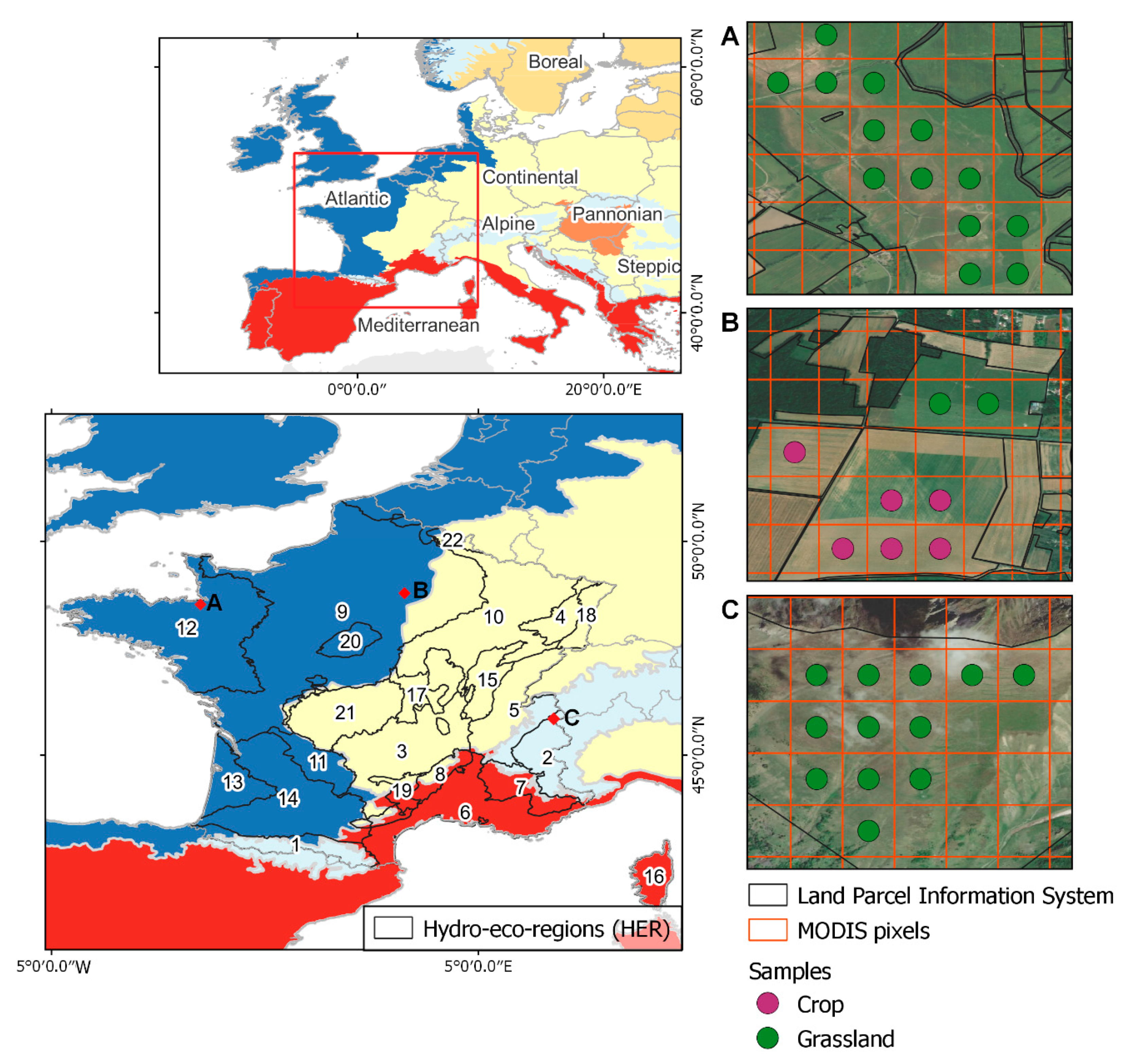
2.1. Study Site

The study focuses on metropolitan France (western Europe), which covers an area of ca. 550,000 km² (Figure 1). National agricultural statistics indicate that, in 2016, grasslands covered nearly 23% of the country [48], representing ca. 42% of the usable agricultural area, compared to 54% in 1970 [3]. France contains much of the diversity in semi-natural European grasslands in the Atlantic, Continental, Mediterranean and Alpine biogeographical regions [49]. For finer delineation, biogeographical regions in France have been divided into 22 “hydro-eco-regions” (HERs) based on the analysis of climatic, geological and topographic layers [50]. The area and fragmentation of grasslands vary among HERs, ranging from small contiguous parcels of a few ha in size separated by hedges in the northwestern wooded landscapes of the Armorican massif (HER 12) or the Central massif (HER 21), to more extended but scattered parcels in the open-field landscapes in the Parisian basin (HER 9), to the extensive mountain pasturelands several hundred ha in size in the Alps (HER 2).

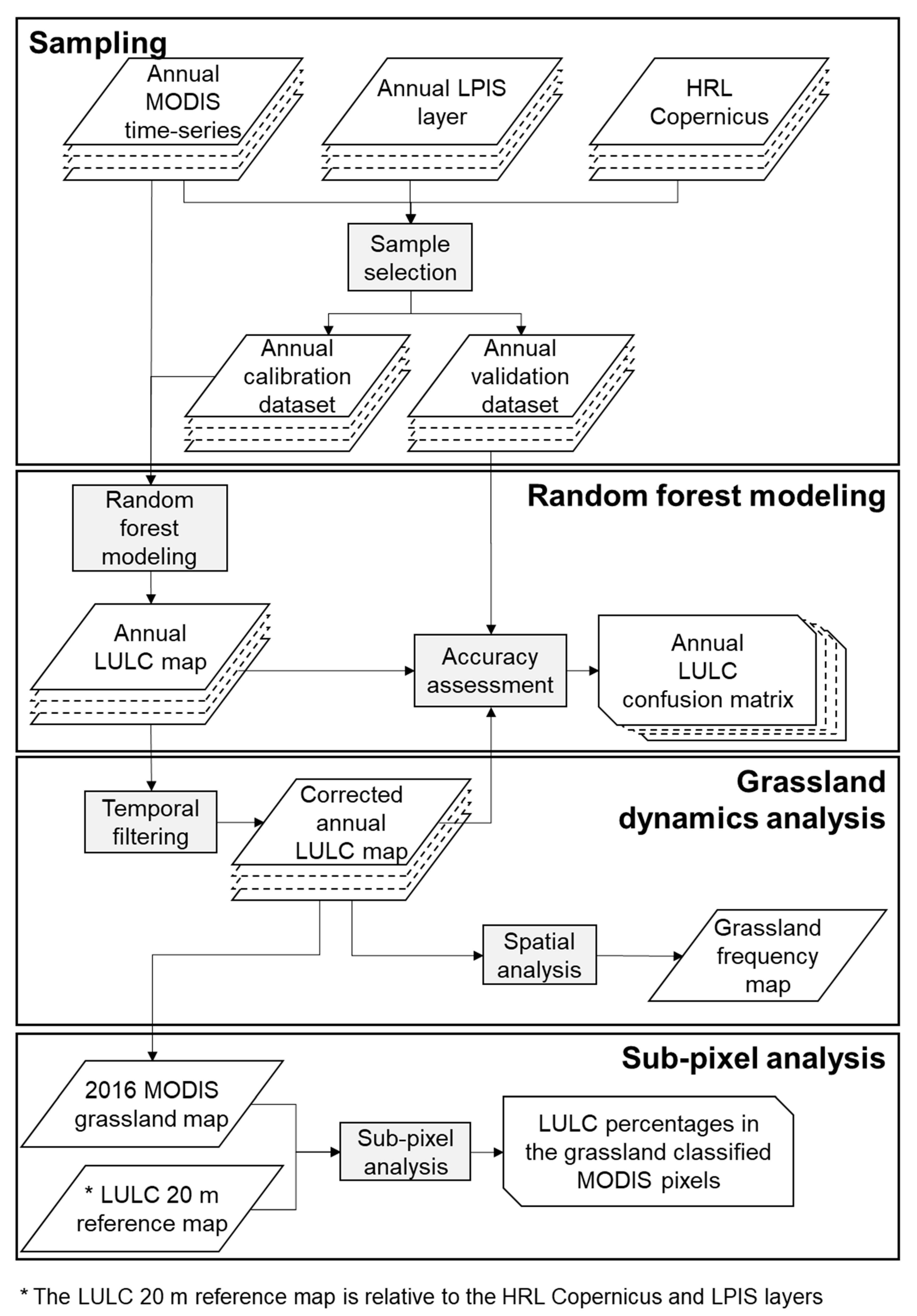
2.2. Rationale of the Approach

The approach first uses RF modeling to identify grasslands each year among the other LULC classes and then combines the annual LULC maps to characterize the spatio-temporal dynamics of grasslands from 2006–2017 (Figure 2). Multi-class modeling (water, woods, urban, crop and grassland) was used instead of single-class modeling (grassland) to prevent arbitrarily selecting a probability threshold for discretizing the grassland class and to quantify over-detection errors [51].

2.3. Data Collection

2.3.1. Satellite Data

The satellite data include MODIS MOD13Q1 and MYD13Q1 composites for the period 2006–2017 (12 years), providing a combined temporal resolution of 8 days [52]. MODIS data from 2003–2005 were not used due to the unavailability of reference data before 2006. These MODIS data were downloaded for the whole of France in WGS84 (EPSG 4326) projection using the USGS Application for Extracting and Exploring and Extracting Analysis Ready Samples (AppEEARS) [53]. We used the red (620–670 nm) and near-infrared (841–876 nm) spectrum bands with a spatial resolution of 250 m. We did not use vegetation indices such as normalized difference vegetation index (NDVI) or enhanced vegetation index (EVI) since they do not increase modeling accuracy significantly [42]. To generate annual grassland maps, MODIS satellite data were stacked by vegetative year, ranging from November 1 of year n to October 30 of year n+1.

Although MOD13Q1 and MYD13Q1 products are cloudless, some pixels had missing values on specific dates, especially in winter, when the days are short and cloudy. To ensure continuous time-series for all pixels, a time interpolation step was required. In this study, the nearest neighbor interpolation method was applied, where missing (NA) values were replaced with the values of the closest date. While the smoothing of the time series restores vegetation phenological profiles [54], the use of raw data was preferred because (i) the dataset consists of a dense time series (8 days) with therefore less missing data than in the 16-day series, (ii) it is still a challenge to discriminate noise from natural variations in vegetation, and part of the information contained in raw time series is lost after filtering [55], and (iii) the contribution of smoothing to the accuracy of LULC classification remains marginal or even negative [56]. The range of pixel values varied with dates and spectral bands, which could lead to the dominance of certain bands in the RF model. Hence, all MODIS pixel values were standardized by setting the overall mean of each spectral band to 0 and the standard deviation to 0.25.

2.3.2. Reference Data

Reference data came from LPIS and Copernicus HRL GIS files (

Table 1. Satellite and reference data used per vegetative year to model land use and land cover (HRL: high-resolution layer).

MOD13Q1 MYD13Q1	Land Parcel Identification System	Water & Wetness HRL	Tree Cover Density HRL	Imperviousness HRL
2005–2006	2006	2015	2012	2006
2006–2007	2007	2015	2012	2006
2007–2008	2008	2015	2012	2006
2008–2009	2009	2015	2012	2009
2009–2010	2010	2015	2012	2009
2010–2011	2011	2015	2012	2009
2011–2012	2012	2015	2012	2012
2012–2013	2013	2015	2012	2012
2013–2014	2014	2015	2012	2012
2014–2015	2015	2015	2015	2015
2015–2016	2016	2015	2015	2015
2016–2017	2017	2015	2015	2015

). The LPIS vector data were collected for each year from 2006–2017 to calibrate and validate modeling of the crop and grassland classes. Unambiguous crop labels 1–15, 20–23 and 25 in the LPIS were assigned to the crop class, while labels 18 (permanent grasslands, more than 5 years old [3]) and 19 (temporary grasslands, 5 years old or less) were assigned to the grassland class (Table S1). In addition, the Copernicus HRL raster data “Water & Wetness”, “Tree Cover Density” and “Imperviousness” were collected to calibrate and validate modeling of the water, woods and urban classes, respectively. These layers, which show the dynamics of LULC in the EU since the 2000s, are produced at a 20 × 20 m spatial resolution from satellite data, such as Landsat-8 or Sentinel, with an overall accuracy above 80% [25]. The “Tree Cover Density” and “Imperviousness” HRLs are expressed as a density of occupancy ranging from 0–1, while the “Water & Wetness” HRL is composed of four classes: (1) permanent water, (2) temporary water, (3) permanent wetness and (4) temporary wetness.

2.4. Data Processing

2.4.1. Sampling

The sampling step aimed to identify and select “pure” MODIS pixels for use as calibration and validation samples for modeling grasslands. First, the footprint of each MODIS pixel was vectorized and overlaid on the reference data. Then, samples were selected for each year from MODIS pixels covering a homogeneous (i.e., single) LULC class (Figure 1). More precisely, the following rules defined the homogeneity criterion:

(i)

A sample of the grassland or crop class is a MODIS pixel strictly included within a parcel block that contains only grassland or one crop type (i.e., it covers >80% of the pixel’s area), respectively [57];

(ii)

A sample of the woods or urban class is a MODIS pixel with >85% of its area covered by a density of “Tree Cover Density” or “Imperviousness” HRL >0.8, respectively. Indeed, since “Tree Cover Density” and “Imperviousness” HRL products are expressed in density values from 0 to 1, a threshold value (0.8) was set to discriminate between wooded (or urban) areas and non-wooded (or non-urban) areas;

(iii)

A sample of the water class is a MODIS pixel with >90% of its area covered by the (1) permanent water class of the “Water & Wetness” HRL. Temporary water (2), permanent wetness (3) and temporary wetness (4) classes were discarded because they can characterize either water areas or grasslands.

The sample spatial density was very heterogeneous throughout France, which could lead to over-representation of some regions in RF modeling. To overcome this issue, sub-sampling was used, with only one sample being kept per mesh of 5 × 5 km per class and per year. For each sample of year n, spectral values were extracted from the MODIS pixels of year n. The number of samples used per year ranged from 21,703–24,565 for all LULC classes, of which 4394–5974 were of the grassland class (Table S2). Then, for each year, the samples were divided randomly and equally per class into a calibration and a validation dataset.

2.4.2. Random Forest Modeling

The RF modeling step identified areas covered by grassland each year. To this end, the five LULC classes (water, urban, woods, crop and grassland) were modeled annually from 2006–2017. For each year, a RF model was applied to the annual MODIS time-series and calibrated with the calibration dataset using a 10-fold approach with three repeats [58]. The maximum number of trees (ntree) was set to 500. Tuning was applied to define the optimal number of variables used for each branch of the RF model tree (mtry) based on the highest Kappa value [59]. Independent validation was performed for each year by applying the RF model to the validation set and calculating three metrics: overall accuracy, the Kappa index and the F1-score of the grassland class. To highlight spatial variation in modeling accuracy, the F1-score of the grassland class was also calculated by biogeographical region.

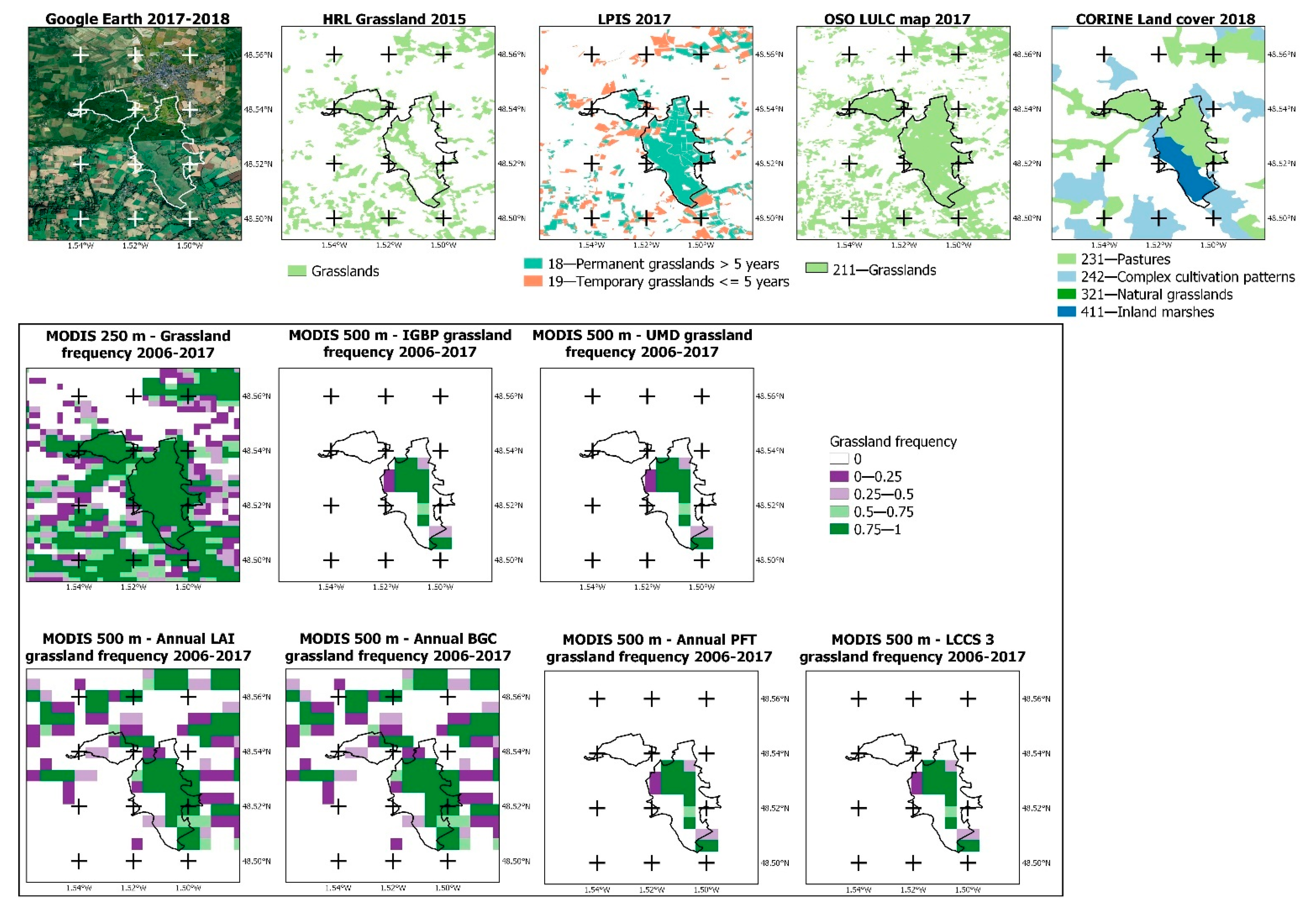
2.4.3. Grassland Dynamics Analysis

The next step analyzed the spatio-temporal dynamics of grasslands by combining the annual LULC maps derived from the RF modeling. To identify and correct illogical LULC transitions, we applied a temporal filter using the approach developed by Clark et al. [60]. For example, it is impossible for a pixel classified as crop one year to be classified as urban the next year and then to return to the crop class two years later. Conversely, a pixel can change from grassland to crop and then back to grassland, depending on the agricultural practices. To this end, we applied transition rules in a 3-year moving window (year n, n+1, and n+2) for each pixel starting in 2006 and repeating it annually until 2017 (

Table 2. Transitional rules used in the temporal filtering. The filter was a 3-year moving window through each map pixel, starting in 2006 and ending in 2017. “Yes” indicates a possible class transition in year n+1, while “No” indicates an illogical class transition.

Years	Class	Year n+1
		Urban	Water	Wood	Crop	Grassland
n and n+2	Urban	Yes	No	No	No	No
	Water	No	Yes	No	No	No
	Woods	No	No	Yes	No	No
	Crop	No	No	No	Yes	Yes
	Grassland	No	No	No	Yes	Yes

). In detail, the filter inspected each pixel to determine whether it had the same class in years n and n+2; if so, and if the class in year n+1 created an illogical transition, then the class in year n+1 was corrected to equal the class in year n. The filter was then advanced by one year in the time-series and the corrected classes of previous years were considered when applying the transition rules.

A pixel’s grassland frequency was calculated by summing the number of years that it was classified as grassland from 2006–2017, and the frequency values were then scaled to a [0–1] range to facilitate result interpretation (12). To visualize this layer’s thematic contribution, its grassland classification was compared to those of national, European and global LULC layers for the lower Couesnon marshes, a Natura 2000 site near Mont-Saint-Michel (HER 12). This site is dominated by natural grassland habitats [43]. In total, five GIS layers were collected:

(i)

The components “231—Pastures”, “242—Complex cultivation patterns”, “321—Natural grasslands” and “411—Inland marshes” of the 2018 CORINE Land Cover layer;

(ii)

The “grassland” HRL of the 2015 Copernicus layers;

(iii)

The “18—Permanent grasslands” and “19—Temporary grasslands” components of the 2016 LPIS layer;

(iv)

The “211—Grasslands” component of the 2018 French national LULC layer (“OSO”) [23];

(v)

The grassland frequency maps, calculated for the period 2006–2017 for each of the six MODIS MCD12Q1 v6 products at 500 m spatial resolution (“IGBP”,”UDM”, “Annual LAI”, “Annual BGC”, “Annual PFT”, and “LCCS 3”) [40].

2.4.4. Sub-Pixel Analysis

Since MODIS data have a coarse spatial resolution (250 m), the pixels classified as grassland have, at a finer scale, LULC diversity that varies according to the landscape. The objective of the sub-pixel analysis step was to quantify the LULC composition of MODIS pixels classified as grassland from a fine-scale reference LULC layer. This reference layer was generated in raster format at 20 m resolution by combining (i) the parcels identified as crop and grassland (i.e., permanent and temporary grasslands) classes in the 2016 LPIS, (ii) the areas classified as permanent and temporary water in the 2015 “Water & Wetness” HRL, (iii) the urban areas classified with a density >0.8 in the 2015 “Imperviousness” HRL and (iv) the woody areas classified with a density >0.8 in the 2015 “Tree Cover Density” HRL. Areas without information in the reference layer (e.g., a woods density <0.8, agricultural parcels not described by the LPIS) were described as mixed. For each pixel of the 20 m reference map, the majority LULC class relative to the HRL Copernicus and LPIS layer has been assigned. The reference layer was then intersected with the grassland layer modeled from the 2016 MODIS data corrected by the temporal filter. MODIS 250 m pixels modeled as grassland with a mixed percentage >20% were discarded. The LULC composition of MODIS pixels classified as grassland was measured as a percentage of MODIS pixel area per HER.

All analyses were performed with R software (version 3.4.3) [28] using the “caret” [59], “raster” [61], “velox” [62] and “rgdal” [63] packages.

3. Results

3.1. Identification of Grasslands

The accuracy of RF modeling of the five LULC classes from 2006–2017 was high, regardless of the year considered (overall accuracy ranging from 0.93 to 0.96, Kappa index ranging from 0.91 to 0.94), especially for the grassland class (F1-score ranging from 0.89 to 0.93) (

Table 3. Overall accuracy, Kappa index and F1-score for the grassland class per year before and after temporal filtering (the highest value for each year and each accuracy metric is in bold).

Year	Overall Accuracy		Kappa Index		F1-Score
	Before Filtering	After Filtering	Before Filtering	After Filtering	Before Filtering	After Filtering
2006	0.96	NA	0.94	NA	0.94	NA
2007	0.95	0.96	0.94	0.94	0.93	0.93
2008	0.92	0.93	0.89	0.91	0.89	0.90
2009	0.93	0.95	0.91	0.92	0.90	0.91
2010	0.93	0.94	0.90	0.92	0.89	0.90
2011	0.93	0.94	0.91	0.92	0.90	0.91
2012	0.93	0.94	0.90	0.92	0.88	0.89
2013	0.93	0.95	0.91	0.92	0.90	0.91
2014	0.93	0.94	0.90	0.92	0.89	0.90
2015	0.94	0.94	0.92	0.92	0.90	0.90
2016	0.93	0.95	0.91	0.93	0.88	0.90
2017	0.94	NA	0.91	NA	0.89	NA

). Temporal filtering increased the accuracy of the five LULC classes slightly (+ 0–0.02 for overall accuracy, + 0–0.02 for the Kappa index), specifically of the grassland class (+ 0–0.02 for the F1-score). Analysis of the 12 annual confusion matrices highlighted confusion among the grassland, crop and woods classes. More precisely, most under-detections of the grassland class (producer’s accuracy 87.8% ± 2.3) were due to confusion with the crop (6.5% ± 1.6) and woods (5.1% ± 1.0) classes, as were most of the over-detections (user’s accuracy 93.8% ± 1.0) (crop 3.2% ± 0.6, woods 1.0% ± 0.2) (Table S7)

From a geographical perspective, the modeling accuracy of the grassland class differed by biogeographical region, with an excellent mean F1-score for the Continental (0.94 ± 0.01) and Atlantic (0.90 ± 0.02) regions, a very good score for the Alpine (0.86 ± 0.04) region and a moderate score (0.62 ± 0.10) for the Mediterranean region. Specifically, grasslands were slightly under-detected (producer’s accuracy 88% ± 3.0) in the Atlantic region, mainly due to confusion with the crop class (9.0% ± 2.2), and rarely over-detected (user’s accuracy 91.8% ± 1.6), again mainly due to the crop class (3.1% ± 0.7) (Table S8). The modeling accuracy for grasslands was similar for the Continental region, with little under-detection error (producer’s accuracy 92.2% ± 1.4), mainly due to confusion with the woods class (5.0% ± 0.9), and little over-detection error (user’s accuracy 96.0% ± 0.6), mainly due to confusion with the crop class (3.6% ± 0.9) (Table S9). The classes confused differed for the Alpine region, with a slightly higher under-detection error for grasslands (producer’s accuracy 79% ± 5.0), mainly due to confusion with the woods class (18.7% ± 4.4), and little over-detection error (user’s accuracy 94.0% ± 2.0), mainly due to confusion with the water class (2.7% ± 2.8) (Table S10). Conversely, the Mediterranean region had distinct results, with a high under-detection error for grasslands (producer’s accuracy 49.4% ± 11.9), mainly due to confusion with the urban (6.6% ± 3.1), woods (17.7% ± 3.8) and crop (25.0% ± 8.5) classes, but little over-detection error (user’s accuracy 86.9% ± 5.0), mainly due to confusion with the crop class (3.8% ± 1.9) (Table S11).

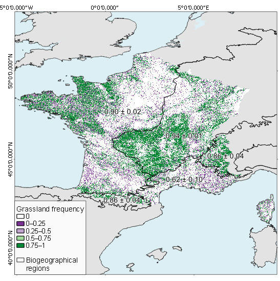
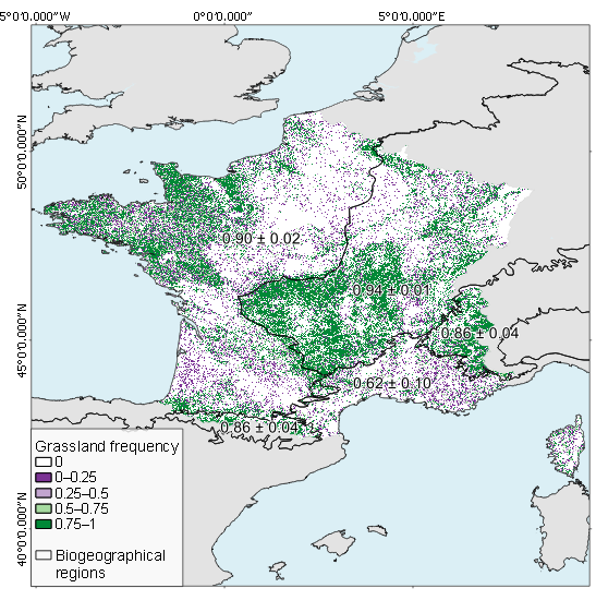
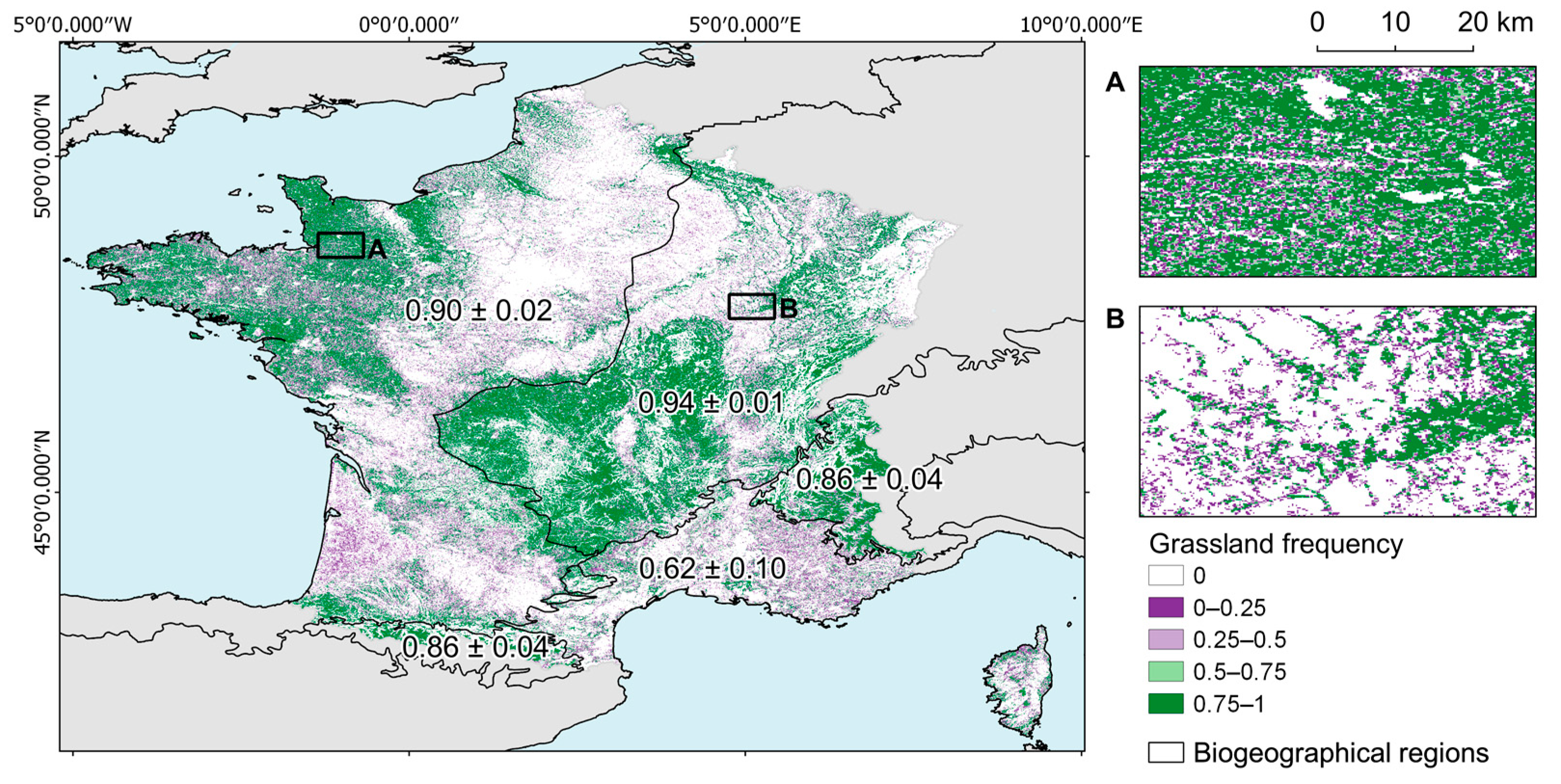
3.2. Characterization of Grassland Frequency

The map of grassland frequency in France derived from annual LULC maps from 2006–2017 illustrates areas where grassland frequency was high, such as hedged landscapes in the Armorican massif (HER 12), the Ardennes (HER 22) and the Central massif (HER 21), and mountain pastures in the Pyrenees (HER 2) and the Alps (HER 1) (Figure 3). Conversely, grassland frequency was low on large cereal plains, such as Alsace (HER 18), the Paris basin (HER 9) and the Aquitaine basin (HER 14). In detail, the map also indicated spatial imbrication of permanent (frequency >0.8) and temporary (frequency <0.5) grasslands in the Normandy bocage (HER 12, Figure 3A) and the residual occurrence of permanent grasslands along valleys in the open-field landscape of the Coteaux calcaires de l’Est (HER 10, Figure 3B).

The grassland frequency map for the lower Couesnon Natura 2000 site consistently showed that it had a high frequency of grassland, although edges of the marshes were unclear due to the low spatial resolution of the MODIS data (Figure 4). In comparison, the CORINE Land Cover layer adequately identified the natural grasslands of the lower Couesnon, but ambiguously classified them as “231—Pastures”, “242—Complex cultivation patterns” or “411—Inland marshes” and not as “321—Natural grasslands”. The grassland HRL under-detected most natural grasslands, especially those that are flooded several months each year, and did not discriminate between temporary and natural grasslands. The LPIS correctly classified natural grasslands as “18—Permanent grasslands”, but with incomplete mapping, since the western end of the marshes (48.54°N, 1.54°W)—not under the EU CAP—is missing. Finally, the national land cover layer “OSO” best identified grasslands, but its classification (“211—Grasslands”) could not discriminate between semi-natural and temporary grasslands. The comparison of the grassland frequency maps derived from the MCD12Q1 v6 products with the Google Earth image and CORINE Land Cover map (Figure 4) points out—beyond the coarse spatial resolution of the MCD12Q1 v6 products—a very strong under-detection of grasslands of the IGBP, UMD, Annual FTP and LCCS 3 maps, and a strong under-detection and strong over-detection of grasslands for the Annual LAI and Annual BGC maps.

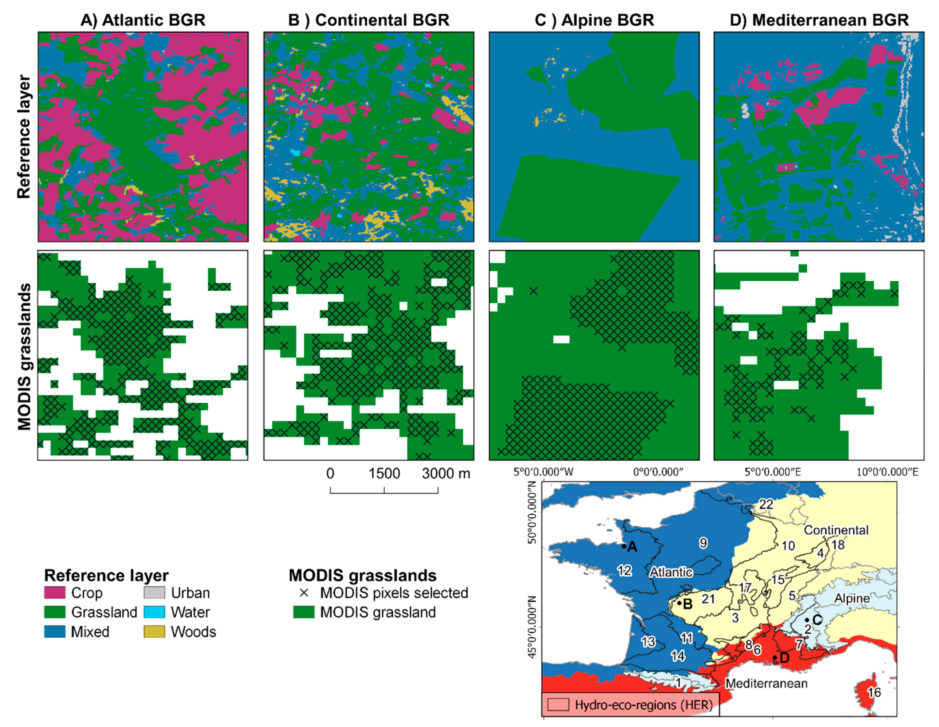
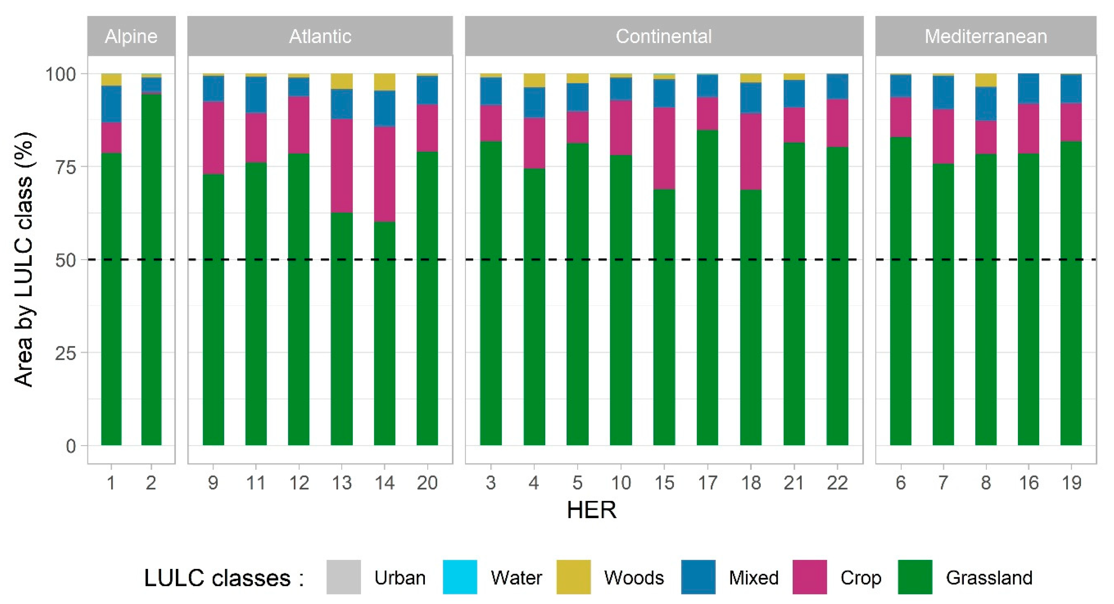
3.3. Land Cover Percentages in MODIS Pixels Classified as Grassland

Comparing the 2016 LULC classification at 250 m spatial resolution to the reference layer at 20 m spatial resolution resulted in the selection of 1,612,318 MODIS pixels—ca. 18% of the total area of France (Figure 5). In the MODIS pixels classified as grassland throughout France in 2016, the grassland class was dominant on all HERs (60%–94%), followed by the crop (0%–25%), mixed (4%–10%) and woods classes (0%–4%). The water and urban classes were negligible (<1%) (Figure 6).

Nonetheless, analysis by biogeographical region identified differences in grassland area among HERs. The Alpine region had the highest percentages of grassland area, both in the Pyrenees (HER 1) and the Alps (HER 2) (77% and 94%, respectively). The percentage of crop area was low (8%) in the Pyrenees and negligible (<1%) in the Alps. The Atlantic region had less grassland dominance and a relatively high percentage of crop area. Specifically, the Landes (HER 13) and Aquitaine coteaux (HER 14) had the lowest percentage of grassland area (62% and 60%, respectively) but the highest percentage of crop and wooded areas (25% and 4%, respectively). Conversely, the percentage of grassland area was higher in the Armorican massif (HER 12) and Sologne (HER 20) (78% each). The Continental region had a high percentage of grassland area, especially in the Central massif (HER 3, 17 and 21; 82%, 81% and 85%, respectively) and the Ardennes (HER 22; 80%). The percentage of crop area was low (8%–15%), except in Alsace (HER 18) and the Saône plain (HER 15) (20% and 22%, respectively). The percentage of wooded area was generally low (0%–2%), except in the Jura (HER 5) and Vosges (HER 4) mountains (4% and 3%, respectively). MODIS pixels classified as grassland in the Mediterranean region had a high percentage of grassland area (76%–83%), while the percentage of crop area was moderate (9%–15%). The wooded area was smallest (<1%), excluding the Cévennes massif (HER 8) (4%).

4. Discussion

4.1. Can MODIS 250 m Time-Series Combined with the RF Classifier Discriminate Grasslands from Other LULC Types at the National Scale?

Overall, the RF classification of MODIS 250 m time-series accurately mapped grasslands each year from 2006–2017 at the scale of France (F1-score 0.89–0.93). These results confirm the advantage of using the RF classifier to discriminate between grasslands [1], which in France are of different types (temporary, wet, mesic, dry or alpine) and thus have different spectral patterns, as well as to manage high-dimensional data (2 spectral bands × 46 dates per year) [46]. For comparison, the overall accuracy of the RF classification applied at the national scale (0.93–0.96) is similar to that obtained using annual MODIS time-series at the regional scale for the Midlands Region of Ireland (0.92) [38] or the Grenoble Alpine region (0.88) [39]. Due to the very high temporal resolution of MODIS images (46 dates/year), the general error rate of classification between grassland and crop classes was low (± 5%) (Table S7). However, the confusion between grassland and crop classes, which was the main source of error at the national scale, reflects the strong similarity in spectral patterns between certain crops and temporary grasslands sown throughout the year [26]. Moreover, the dates of the reference data for the Water & Wetness HRL (2015) and Tree Cover Density HRL (2012 and 2015) differ up to 10 years from the dates of MOD13Q1 and MYD13Q1 products (2006–2017). Although forests, rivers and water bodies are relatively stable over time, changes in LULCs could have occurred between 2006 and 2015, which may lead to classification errors.

The use of “pure” pixels for validation may lead to a slight overestimation of the classification accuracy. However, the use of “mixed” pixels would probably underestimate the classification accuracy. In any case, given the large number of samples used per year (± 12,000), the sample quality (farmers’ declarations), sample independence (from training samples) and their homogeneous distribution throughout the territory (sub-sampling 5 × 5 km), the estimated classification accuracy is considered reliable.

At the regional scale, while grasslands were classified with great accuracy in the Atlantic and Continental biogeographical regions (F1-score 0.90 and 0.94, respectively)—which cover most of France—more errors were observed in the Alpine (F1-score 0.86) and Mediterranean (F1-score 0.62) regions. In the Alpine region, confusion was observed mainly between the grassland and woods classes (± 18%). This could be because many parcels described as “grassland” in this region in the LPIS include moorland facies with a strong mixture of grassland and woods, which are difficult to discriminate using remote sensing [23]. The Mediterranean region was the least accurately modeled, with a significant under-detection of grasslands. The facies of many Mediterranean grasslands are similar to those of scrubland with a low percentage of ground cover and sometimes the presence of many shrubs [64]. This would explain why some Mediterranean grasslands were under-estimated due to confusion with the urban and woods classes (Table S11). The confusion between crops and grasslands in the Mediterranean region can be explained by the high proportion of vineyards and orchards that have herbaceous vegetation between the rows of vines or fruit trees. The highly distinctive landscape of the Mediterranean region requires a specific RF model with an adapted nomenclature [65].

The quality of MODIS products used in this study could also explain some of the errors in the grassland classification. The modeling was based on the red and NIR bands of the MOD13Q1 and MYD13Q1 products, which may lead a lower modeling accuracy of grasslands in the Alpine biogeographical region compared to those achieved in the Atlantic and continental lowland regions, since these two spectral bands are sensitive to terrain distortions. However, we chose to use the red and NIR bands rather than the NDVI and EVI of the MOD13Q1 product, because these vegetation indices have some limitations: (i) they reduce spectral dimension from two features (red and NIR bands) to one (NDVI or EVI), which can reduce class separability; (ii) the EVI is computed using the 500 m blue band, which can generate artifacts in images at 250 m spatial resolution; (iii) the NDVI index saturates in high values, while grasslands have high reflectance values in spring and summer. Besides, MOD13Q1 and MYD13Q1 products—which are 16-day composite products—contain inconsistencies in pixel values related to differences in incidence angles and albedo values between the images used to create the composite products. These spectral biases can generate errors in LUCL classification—especially in winter, when atmospheric disturbances are more important. More consistent spectral products with observations every 8 days—time series of globally distributed spectral MODIS NBARs (nadir bidirectional reflectance distribution function adjusted surface reflectance)—are available [66]. However, the low spatial resolution of this product (500 m) would not be appropriate for the detection of the majority of grasslands that were detected using the MOD13Q1 and MYD13Q1 products (250 m).

Sampling can also explain the regional differences in the accuracy of the RF model. Despite the application of 5 × 5 km grid sub-sampling, the Atlantic and Continental regions had more samples than the Alpine and Mediterranean regions since they cover the largest area in France (Tables S3, S4, S5 and S6). As a result, the RF model, which is calibrated with the highest Kappa index [59], discriminated between grasslands in the Atlantic and Continental regions better, since their larger number influenced overall accuracy more than the smaller number of grasslands in the Alpine and Mediterranean regions. The accuracy of RF models is also strongly influenced by the quality of the sampling [46,67]. One of the challenges when analyzing data with moderate spatial resolution, such as MODIS, is selecting enough samples that correspond to “pure” pixels. Samples selected from “mixed” MODIS pixels have a negative influence on classification accuracy [68]. For this reason, we carefully selected only MODIS pixels covering >80% of the same LULC class. This strong sample selection was possible because the LPIS contains a large amount of reference data (i.e., more than 200,000 polygons across France for each year since 2006). Applying this approach outside the EU would be more difficult due to the scarcity of availability of field databases [1,47]. However, using expert-rule classification methods based on annual NDVI time profiles could be an alternative solution to discriminate grasslands from other LULC types in regions where field data are not widely available [47,69].

The grassland maps included in the global MCD12Q1 v6 products were obviously less accurate than the one obtained from MOD13Q1 and MYD13Q1 composites. While the six LULC maps of the MCD12Q1 v6 product were generated by a single RF model applied throughout the planet using about 3,000 reference samples selected by visual interpretation of very high spatial resolution images [40], the MODIS 250 m LULC map was computed at a national scale with one RF model calibrated using about 12,000 reference samples validated in the field. We visually compared these LULC maps on a Natura 2000 site. A thorough statistical comparison performed at a national scale would deserve a dedicated study. The reference data—i.e., pure MODIS pixels at 250 m spatial resolution—produced over the period 2006–2017 from LPIS are publicly available [57] and can be integrated for future global LULC classification.

4.2. Can a Decadal MODIS 250 m Time-Series Identify Semi-Natural Grasslands Based on a Grassland Frequency Map?

The grassland frequency map was derived from MODIS 250 m satellite time-series from 2006–2017. To our knowledge, this is the first study conducted to identify “permanent” grasslands using satellite remote sensing for such a long period (12 years); in comparison, Garcia-Feced et al. [6] and Lasseur et al. [39] monitored grasslands over a 5 or 4-year period, respectively. Given the temporal depth of the analysis (12 years), grasslands identified as permanent (i.e., a frequency close to 1) have a high probability of being semi-natural [2]. Nevertheless, certain 12-year permanent grasslands may be long-term “temporary” grasslands that have not yet restored the floristic composition of semi-natural grasslands [3]. Adding new MODIS images to the time-series (>2017) would yield a longer time-series (20 years) that could address this uncertainty.

The two major limitations of current national and international LULC maps for monitoring semi-natural grasslands are their (i) coarse spatial resolution and (ii) low thematic resolution, which hinder clear correspondence between semi-natural and temporary grasslands [13]. The national grassland frequency map addresses these limitations and improves knowledge about semi-natural grasslands in two ways. First, its 250 m resolution identifies semi-natural grasslands more accurately than maps produced from LPIS or CORINE Land Cover at a spatial resolution of 5 km [22] or from the EVA database at a spatial resolution of 10 km [19]; second, it uses long-term monitoring to discriminate between semi-natural and temporary grasslands, which is something that LULC maps derived from annual time-series analysis of remote sensing data do not do [23,25,30].

However, this grassland frequency map should be read carefully. While interpreting the extreme values (0 and 1) is straightforward, this is less true for intermediate values. First, the analysis does not consider damage to semi-natural grasslands from 2006–2017 that would affect the grassland frequency. For example, a semi-natural grassland converted into an urban area in 2011 would be classified as grassland only from 2006–2010 and would have a frequency of ca. 0.5. Second, although annual grassland modeling was highly successful (F1-score 0.89–0.93), the few errors generated each year may have accumulated when calculating grassland frequency as a aggregation of annual LULC maps [39,70]. Given these issues, the grassland frequency map should be used to help pre-locate semi-natural grasslands rather than as an inventory per se. For example, pre-locating semi-natural grasslands could improve implementation of restoration strategies for agricultural systems and biodiversity in Europe [6].

4.3. Is the 250 m Spatial Resolution of MODIS Data Adequate for Identifying Grasslands in Fragmented Landscapes?

Results of the sub-pixel analysis for 2016 reveal that MODIS images at 250 m spatial resolution successfully identified grassland-dominated areas. These results confirm that MODIS images can detect grasslands in homogeneous landscapes [36,39], such as mountain pastures, and in more fragmented landscapes such as the Armorican massif. Although grassland percentage predominated in all HERs (60%–94%), it may be more appropriate to use the term “grassland landscape” rather than “grassland”. A MODIS pixel classified as grassland generally included 15% of crop area. Conversely, it is likely that some “isolated” and small semi-natural grasslands were classified as crop or woods. Although these results are based on a large sample (ca. 18% of the area of France), they may be biased slightly by (i) the quality and spatial resolution of the reference layers (HRL, LPIS), which do not represent small elements of LULC (e.g. hedges, small water bodies, roads), and (ii) the low—but existing—rates of modeling error (producer’s accuracy 87.8%, user’s accuracy 97.8%).

5. Conclusions

Analysis of MODIS 250 m time-series from 2006–2017 (12 years) for the whole of France revealed the presence of permanent grasslands. This map is a new aid for pre-locating semi-natural grasslands at the national scale. Results demonstrate that a single RF model correctly discriminates between different types of grassland in the Atlantic, Continental and Alpine biogeographical regions, but identifying semi-natural grasslands in the Mediterranean region requires a specific RF model and nomenclature. Although the spatial resolution of MODIS data is coarse compared to parcels sizes, sub-pixel analysis highlights that areas modeled as grassland correspond to grassland-dominant areas. Perspectives of this approach include (i) characterizing grasslands by temporally analyzing their inter-annual spectral profiles using deep-learning approach, (ii) identifying grasslands at a finer scale using Sentinel-1/2 time-series and (iii) monitoring grasslands over a longer period and for the whole of Europe.

References

1. Ali, I.; Cawkwell, F.; Dwyer, E.; Barrett, B.; Green, S. Satellite remote sensing of grasslands: From observation to management. J. Plant Ecol. 2016, 9, 649–671. [Google Scholar] [CrossRef] [Green Version]
2. Allen, V.G.; Batello, C.; Berretta, E.J.; Hodgson, J.; Kothmann, M.; Li, X.; McIvor, J.; Milne, J.; Morris, C.; Peeters, A.; et al. An international terminology for grazing lands and grazing animals. Grass Forage Sci. 2011, 66, 2–28. [Google Scholar] [CrossRef]
3. Plantureux, S.; Pottier, E.; Carrère, P. Permanent grassland: New challenges, new definitions? Fourrages 2012, 2012, 181–193. [Google Scholar]
4. Huguenin-Elie, O.; Delaby, L.; Klumpp, K.; Lemauviel-Lavenant, S.; Ryschawy, J.; Sabatier, R. The role of grasslands in biogeochemical cycles and biodiversity conservation. In Improving Grassland and Pasture Management in Temperate Agriculture; Marshall, A., Collins, R., Eds.; Burleigh Dodds Science Publishing: Cambridge, UK, 2019; p. 486. ISBN 978-1-78676-200-9. [Google Scholar]
5. Maltby, E.; Barker, T. The Wetlands Handbook; Wiley-Blackwell: Oxford, UK, 2009. [Google Scholar]
6. García-Feced, C.; Weissteiner, C.J.; Baraldi, A.; Paracchini, M.L.; Maes, J.; Zulian, G.; Kempen, M.; Elbersen, B.; Pérez-Soba, M. Semi-natural vegetation in agricultural land: European map and links to ecosystem service supply. Agron. Sustain. Dev. 2015, 35, 273–283. [Google Scholar] [CrossRef] [Green Version]
7. Paracchini, M.L.; Petersen, J.-E.; Hoogeveen, Y.; Bamps, C.; Burfield, I.; van Swaay, C. High Nature Value Farmland in Europe—An Estimate of the Distribution Patterns on the Basis of Land Cover and Biodiversity Data; JRC Scientific &Technical Report; European Commission: Luxemburg, 2008; p. 87. [Google Scholar]
8. Council Directive 92/43/EEC Conservation of natural habitats and of wild flora and fauna. Int. J. Eur. Communities 1992, 206, 7–50.
9. Kallis, G.; Butler, D. The EU water framework directive: Measures and implications. Water Policy 2001, 3, 125–142. [Google Scholar] [CrossRef]
10. European Parliament Regulation (EU) No 1307/2013 of the European Parliament and of the Council of 17 December 2013 establishing rules for direct payments to farmers under support schemes within the framework of the common agricultural policy and repealing Council Regulation (EC) No 637/2008 and Council Regulation (EC) No 73/2009. Off. J. Eur. Communities 2013, 347, 608–670.
11. European Parliament Regulation (EU) 2018/841 of the European parliament and of the council of 30 May 2018 on the inclusion of greenhouse gas emissions and removals from land use, land use change and forestry in the 2030 climate and energy framework, and amending Regulation (EU) No 525/2013 and Decision No 529/2013/EU. Off. J. Eur. Union 2018, 156, 1–25.
12. Levin, G. Applying parcel-specific land-use data for improved monitoring of semi-natural grassland in Denmark. Environ. Monit. Assess. 2013, 185, 2615–2625. [Google Scholar] [CrossRef]
13. Lomba, A.; Guerra, C.; Alonso, J.; Honrado, J.P.; Jongman, R.; McCracken, D. Mapping and monitoring High Nature Value farmlands: Challenges in European landscapes. J. Environ. Manag. 2014, 143, 140–150. [Google Scholar] [CrossRef]
14. EUROSTAT Land Use and Coverage Area Frame Survey (LUCAS). 2017. Available online: https://ec.europa.eu/eurostat/web/products-catalogues/-/KS-01-17-069 (accessed on 13 December 2019).
15. Chytrý, M.; Hennekens, S.M.; Jiménez-Alfaro, B.; Knollová, I.; Dengler, J.; Jansen, F.; Landucci, F.; Schaminée, J.H.; Aćić, S.; Agrillo, E.; et al. European Vegetation Archive (EVA): An integrated database of European vegetation plots. Appl. Veg. Sci. 2016, 19, 173–180. [Google Scholar] [CrossRef] [Green Version]
16. Esch, T.; Metz, A.; Marconcini, M.; Keil, M. Combined use of multi-seasonal high and medium resolution satellite imagery for parcel-related mapping of cropland and grassland. Int. J. Appl. Earth Obs. Geoinf. 2014, 28, 230–237. [Google Scholar] [CrossRef]
17. Xiao, Y.; Mignolet, C.; Mari, J.-F.; Benoît, M. Characterizing historical (1992–2010) transitions between grassland and cropland in mainland France through mining land-cover survey data. J. Integr. Agric. 2015, 14, 1511–1523. [Google Scholar] [CrossRef]
18. Zimmermann, J.; González, A.; Jones, M.B.; O’Brien, P.; Stout, J.C.; Green, S. Assessing land-use history for reporting on cropland dynamics—A comparison between the Land-Parcel Identification System and traditional inter-annual approaches. Land Use Policy 2016, 52, 30–40. [Google Scholar] [CrossRef]
19. Schaminée, J.H.; Chytrý, M.; Hennekens, S.M.; Janssen, J.A.; Jiménez-Alfaro, B.; Knollová, I.; Marceno, C.; Mucina, L.; Rodwell, J.S.; Tichý, L. Review of Grassland Habitats and Development of Distribution Maps of Heathland, Scrub and Tundra Habitats of EUNIS habitats Classification. Alterra Institute. 2016. Available online: https://www.google.com/url?sa=t&rct=j&q=&esrc=s&source=web&cd=2&cad=rja&uact=8&ved=2ahUKEwinwPez_7nmAhWYFMAKHSg3BQ8QFjABegQIAxAC&url=https%3A%2F%2Fforum.eionet.europa.eu%2Fnrc-biodiversity%2Flibrary%2Feunis_classification%2Freports%2Freport-2016-eunis-grasslands-review-and-heathland-scrub-tundra-maps%2Fdownload%2Fen%2F2%2FReport%25202016%2520EUNIS%2520grasslands%2520review%2520and%2520heathland-scrub-tundra%2520maps.pdf&usg=AOvVaw3hyAEmebXU3IXHxj9Ylng5 (accessed on 13 December 2019).
20. Wachendorf, M.; Fricke, T.; Möckel, T. Remote sensing as a tool to assess botanical composition, structure, quantity and quality of temperate grasslands. Grass Forage Sci. 2018, 73, 1–14. [Google Scholar] [CrossRef]
21. Feranec, J.; Soukup, T.; Hazeu, G.; Jaffrain, G. European Landscape Dynamics: CORINE Land Cover Data; CRC Press: Boca Raton, FL, USA, 2016; ISBN 1-4822-4468-3. [Google Scholar]
22. Violle, C.; Choler, P.; Borgy, B.; Garnier, E.; Amiaud, B.; Debarros, G.; Diquelou, S.; Gachet, S.; Jolivet, C.; Kattge, J.; et al. Vegetation ecology meets ecosystem science: Permanent grasslands as a functional biogeography case study. Sci. Total Environ. 2015, 534, 43–51. [Google Scholar] [CrossRef]
23. Inglada, J.; Vincent, A.; Arias, M.; Tardy, B.; Morin, D.; Rodes, I. Operational High Resolution Land Cover Map Production at the Country Scale Using Satellite Image Time Series. Remote Sens. 2017, 9, 95. [Google Scholar]
24. Lopes, M.; Fauvel, M.; Girard, S.; Sheeren, D. Object-based classification of grasslands from high resolution satellite image time series using Gaussian mean map kernels. Remote Sens. 2017, 9, 688. [Google Scholar] [CrossRef] [Green Version]
25. Büttner, G.; Maucha, G.; Kosztra, B. High-Resolution Layers. In European Landscape Dynamics: CORINE Land Cover Data; CRC Press: Boca Raton, FL, USA, 2016; pp. 61–70. [Google Scholar]
26. Dusseux, P.; Vertès, F.; Corpetti, T.; Corgne, S.; Hubert-Moy, L. Agricultural practices in grasslands detected by spatial remote sensing. Environ. Monit Assess. 2014, 186, 8249–8265. [Google Scholar] [CrossRef]
27. Schuster, C.; Schmidt, T.; Conrad, C.; Kleinschmit, B.; Förster, M. Grassland habitat mapping by intra-annual time series analysis – Comparison of RapidEye and TerraSAR-X satellite data. Int. J. Appl. Earth Obs. Geoinf. 2015, 34, 25–34. [Google Scholar] [CrossRef]
28. Franke, J.; Keuck, V.; Siegert, F. Assessment of grassland use intensity by remote sensing to support conservation schemes. J. Nat. Conserv. 2012, 20, 125–134. [Google Scholar] [CrossRef]
29. Xu, D.; Chen, B.; Shen, B.; Wang, X.; Yan, Y.; Xu, L.; Xin, X. The Classification of Grassland Types Based on Object-Based Image Analysis with Multisource Data. Rangel. Ecol. Manag. 2019, 72, 318–326. [Google Scholar] [CrossRef]
30. Palchowdhuri, Y.; Valcarce-Diñeiro, R.; King, P.; Sanabria-Soto, M. Classification of multi-temporal spectral indices for crop type mapping: A case study in Coalville, UK. J. Agric. Sci. 2018, 156, 24–36. [Google Scholar] [CrossRef]
31. Rapinel, S.; Fabre, E.; Dufour, S.; Arvor, D.; Mony, C.; Hubert-Moy, L. Mapping potential, existing and efficient wetlands using free remote sensing data. J. Environ. Manag. 2019, 247, 829–839. [Google Scholar] [CrossRef] [PubMed]
32. Bégué, A.; Arvor, D.; Bellon, B.; Betbeder, J.; De Abelleyra, D.; P. D. Ferraz, R.; Lebourgeois, V.; Lelong, C.; Simões, M.; R. Verón, S. Remote Sensing and Cropping Practices: A Review. Remote Sens. 2018, 10, 99. [Google Scholar]
33. Rapinel, S.; Dusseux, P.; Bouzillé, J.-B.; Bonis, A.; Lalanne, A.; Hubert-Moy, L. Structural and functional mapping of geosigmeta in Atlantic coastal marshes (France) using a satellite time series. Plant. Biosyst. Int. J. Deal. All Asp. Plant Biol. 2018, 152, 1101–1108. [Google Scholar] [CrossRef]
34. Dabrowska-Zielinska, K.; Budzynska, M.; Gatkowska, M.; Kowalik, W.; Bartold, M.; Kiryla, M. Importance of grasslands monitoring applying optical and radar satellite data in perspective of changing climate. In Proceedings of the 2017 IEEE International Geoscience and Remote Sensing Symposium (IGARSS), Fort Worth, TX, USA, 23–28 July 2017; pp. 5782–5785. [Google Scholar]
35. Estel, S.; Mader, S.; Levers, C.; Verburg, P.H.; Baumann, M.; Kuemmerle, T. Combining satellite data and agricultural statistics to map grassland management intensity in Europe. Environ. Res. Lett. 2018, 13, 074020. [Google Scholar] [CrossRef]
36. Halabuk, A.; Mojses, M.; Halabuk, M.; David, S. Towards Detection of Cutting in Hay Meadows by Using of NDVI and EVI Time Series. Remote Sens. 2015, 7, 6107–6132. [Google Scholar] [CrossRef] [Green Version]
37. Fassnacht, F.E.; Schiller, C.; Qu, J.; Kattenborn, T.; Zhao, X. Modis-Based Grassland Trends Within and Around the Kekexili Core Protection Zone of the Sanjiangyuan Nature Reserve. In Proceedings of the IGARSS 2018—2018 IEEE International Geoscience and Remote Sensing Symposium, Valencia, Spain, 22–27 July 2018; pp. 2880–2882. [Google Scholar]
38. Nitze, I.; Barrett, B.; Cawkwell, F. Temporal optimisation of image acquisition for land cover classification with Random Forest and MODIS time-series. Int. J. Appl. Earth Obs. Geoinf. 2015, 34, 136–146. [Google Scholar] [CrossRef] [Green Version]
39. Lasseur, R.; Vannier, C.; Lefebvre, J.; Longaretti, P.-Y.; Lavorel, S. Landscape-scale modeling of agricultural land use for the quantification of ecosystem services. J. Appl. Remote Sens. 2018, 12, 046024. [Google Scholar] [CrossRef]
40. Sulla-Menashe, D.; Gray, J.M.; Abercrombie, S.P.; Friedl, M.A. Hierarchical mapping of annual global land cover 2001 to present: The MODIS Collection 6 Land Cover product. Remote Sens. Environ. 2019, 222, 183–194. [Google Scholar] [CrossRef]
41. Vuolo, F.; Atzberger, C. Improving Land Cover Maps in Areas of Disagreement of Existing Products using NDVI Time Series of MODIS–Example for Europe. Photogramm. Fernerkund. Geoinf. 2014, 2014, 393–407. [Google Scholar] [CrossRef]
42. Khatami, R.; Mountrakis, G.; Stehman, S.V. A meta-analysis of remote sensing research on supervised pixel-based land-cover image classification processes: General guidelines for practitioners and future research. Remote Sens. Environ. 2016, 177, 89–100. [Google Scholar] [CrossRef] [Green Version]
43. Betbeder, J.; Rapinel, S.; Corpetti, T.; Pottier, E.; Corgne, S.; Hubert-Moy, L. Multitemporal classification of TerraSAR-X data for wetland vegetation mapping. J. Appl. Remote Sens 2014, 8, 083648. [Google Scholar] [CrossRef]
44. Dedieu, J.-P.; Carlson, B.Z.; Bigot, S.; Sirguey, P.; Vionnet, V.; Choler, P. On the Importance of High-Resolution Time Series of Optical Imagery for Quantifying the Effects of Snow Cover Duration on Alpine Plant Habitat. Remote Sens. 2016, 8, 481. [Google Scholar] [CrossRef] [Green Version]
45. Féret, J.B.; Corbane, C.; Alleaume, S. Detecting the Phenology and Discriminating Mediterranean Natural Habitats With Multispectral Sensors—An Analysis Based on Multiseasonal Field Spectra. IEEE J. Sel. Top. Appl. Earth Obs. Remote Sens. 2015, 8, 2294–2305. [Google Scholar] [CrossRef]
46. Belgiu, M.; Drăguţ, L. Random forest in remote sensing: A review of applications and future directions. ISPRS J. Photogramm. Remote Sens. 2016, 114, 24–31. [Google Scholar] [CrossRef]
47. Massey, R.; Sankey, T.T.; Congalton, R.G.; Yadav, K.; Thenkabail, P.S.; Ozdogan, M.; Sánchez Meador, A.J. MODIS phenology-derived, multi-year distribution of conterminous U.S. crop types. Remote Sens. Environ. 2017, 198, 490–503. [Google Scholar] [CrossRef]
48. AGRESTE. Enquête Prairies-Résultats. 2017. Available online: http://agreste.agriculture.gouv.fr/conjoncture/grandes-cultures-et-fourrages/prairies/ (accessed on 13 December 2019).
49. European Environment Agency. Biogeographical Regions. 2016. Available online: https://www.eea.europa.eu/data-and-maps/data/biogeographical-regions-europe-3 (accessed on 13 December 2019).
50. Wasson, J.G.; Chandesris, A.; Pella, H.; Blanc, L. Les hydro-écorégions: Une approche fonctionnelle de la typologie des rivières pour la Directive cadre européenne sur lèau. Ingénieries EAT 2004, 40, 3–10. [Google Scholar]
51. Stenzel, S.; Feilhauer, H.; Mack, B.; Metz, A.; Schmidtlein, S. Remote sensing of scattered Natura 2000 habitats using a one-class classifier. Int. J. Appl. Earth Obs. Geoinf. 2014, 33, 211–217. [Google Scholar] [CrossRef]
52. Solano, R.; Didan, K.; Jacobson, A.; Huete, A. MODIS Vegetation Index User’s Guide (MOD13 Series). Vegetation Index and Phenology Lab. The University of Arizona. 2010, pp. 1–38. Available online: https://vip.arizona.edu/documents/MODIS/MODIS_VI_UsersGuide_01_2012.pdf (accessed on 13 December 2019).
53. Neeley, S. Analyzing Earth Data with NASA’s AppEEARS Tool to Improve Research Efficiency. In Proceedings of the AGU Fall Meeting Abstracts, Washington, DC, USA, 10–14 December 2018. [Google Scholar]
54. Atkinson, P.M.; Jeganathan, C.; Dash, J.; Atzberger, C. Inter-comparison of four models for smoothing satellite sensor time-series data to estimate vegetation phenology. Remote Sens. Environ. 2012, 123, 400–417. [Google Scholar] [CrossRef]
55. Picoli, M.C.A.; Camara, G.; Sanches, I.; Simões, R.; Carvalho, A.; Maciel, A.; Coutinho, A.; Esquerdo, J.; Antunes, J.; Begotti, R.A. Big earth observation time series analysis for monitoring Brazilian agriculture. ISPRS J. Photogramm. Remote Sens. 2018, 145, 328–339. [Google Scholar] [CrossRef]
56. Shao, Y.; Lunetta, R.S.; Wheeler, B.; Iiames, J.S.; Campbell, J.B. An evaluation of time-series smoothing algorithms for land-cover classifications using MODIS-NDVI multi-temporal data. Remote Sens. Environ. 2016, 174, 258–265. [Google Scholar] [CrossRef]
57. Hubert-Moy, L.; Thibault, J.; Fabre, E.; Rozo, C.; Arvor, D.; Corpetti, T.; Rapinel, S. Time-series spectral dataset for croplands in France (2006–2017). Data Brief 2019, 27, 104810. [Google Scholar] [CrossRef] [PubMed]
58. Kuhn, M.; Johnson, K. Applied Predictive Modeling; Springer: New York, NY, USA, 2013; ISBN 978-1-4614-6848-6. [Google Scholar]
59. Kuhn, M. Caret package. J. Stat. Softw. 2008, 28, 1–26. [Google Scholar]
60. Clark, M.L.; Aide, T.M.; Grau, H.R.; Riner, G. A scalable approach to mapping annual land cover at 250 m using MODIS time series data: A case study in the Dry Chaco ecoregion of South America. Remote Sens. Environ. 2010, 114, 2816–2832. [Google Scholar] [CrossRef]
61. Hijmans, R.J. Raster: Geographic Data Analysis and Modeling; R Package Version 3.0. 2019. Available online: https://cran.r-project.org/web/packages/raster/index.html (accessed on 13 December 2019).
62. Hunziker, P. Velox: Fast Raster Manipulation and Extraction, R Package Version 0.2. 0. 2017. Available online: https://cran.r-project.org/web/packages/velox/velox.pdf (accessed on 13 December 2019).
63. Bivand, R.; Keitt, T.; Rowlingson, B. Rgdal: Bindings for the Geospatial Data Abstraction Library. 2015. Available online: https://cran.r-project.org/web/packages/rgdal/index.html (accessed on 13 December 2019).
64. Davies, C.E.; Moss, D.; Hill, M.O. EUNIS Habitat Classification Revised 2004. European Environment Agency European Topic Centre on Nature Protection and Biodiversity. 2004. Available online: https://inpn.mnhn.fr/docs/ref_habitats/Davies_&_Moss_2004_EUNIS_habitat_classification.pdf (accessed on 13 December 2019).
65. Pelletier, C.; Valero, S.; Inglada, J.; Champion, N.; Dedieu, G. Assessing the robustness of Random Forests to map land cover with high resolution satellite image time series over large areas. Remote Sens. Environ. 2016, 187, 156–168. [Google Scholar] [CrossRef]
66. Schaaf, C.B.; Gao, F.; Strahler, A.H.; Lucht, W.; Li, X.; Tsang, T.; Strugnell, N.C.; Zhang, X.; Jin, Y.; Muller, J.-P. First operational BRDF, albedo nadir reflectance products from MODIS. Remote Sens. Environ. 2002, 83, 135–148. [Google Scholar] [CrossRef] [Green Version]
67. Maxwell, A.E.; Warner, T.A.; Fang, F. Implementation of machine-learning classification in remote sensing: An applied review. Int. J. Remote Sens. 2018, 39, 2784–2817. [Google Scholar] [CrossRef] [Green Version]
68. Pouliot, D.; Latifovic, R.; Zabcic, N.; Guindon, L.; Olthof, I. Development and assessment of a 250 m spatial resolution MODIS annual land cover time series (2000–2011) for the forest region of Canada derived from change-based updating. Remote Sens. Environ. 2014, 140, 731–743. [Google Scholar] [CrossRef]
69. Nguyen, L.H.; Henebry, G.M. Characterizing Land Use/Land Cover Using Multi-Sensor Time Series from the Perspective of Land Surface Phenology. Remote Sens. 2019, 11, 1677. [Google Scholar] [CrossRef] [Green Version]
70. Mueller-Warrant, G.W.; Sullivan, C.; Anderson, N.; Whittaker, G.W. Detecting and correcting logically inconsistent crop rotations and other land-use sequences. Int. J. Remote Sens. 2016, 37, 29–59. [Google Scholar] [CrossRef]
Figure 1. Study site and data description, showing (left) borders of the four European biogeographical regions and 22 hydro-eco-regions (HER) covering France and (right) selection of crop and grassland class samples within Moderate Resolution Imaging Spectroradiometer (MODIS) 250 m pixels and parcels boundaries in (A) a hedged landscape, (B) an open-field landscape and (C) an Alpine landscape.
Remotesensing 11 03041 g001
Figure 2. Methodological flowchart (LPIS: Land Parcel Information System, HRL: hgigh-resolution layer, LULC: land-use and land-cover).
Remotesensing 11 03041 g002
Figure 3. Frequency of grassland years from 2006–2017 across France derived from 250 m MODIS satellite data, ranging from 1 (permanent grasslands) to zero (non-grassland areas). Values on the map show the mean and standard deviation of F1-scores for each biogeographical region. Inset maps show detail of (A) the Normandy bocage and (B) the Coteaux calcaires de l’Est.
Remotesensing 11 03041 g003
Figure 4. Comparison of the grassland frequency map derived from MODIS data (2006–2017) to existing GIS layers that identify grasslands for the Natura 2000 site of the Couesnon low marshes (black outlines) (in FR2510048) (see Betbeder et al. [43] for a detailed description).
Remotesensing 11 03041 g004
Figure 5. Illustration of MODIS pixels classified as grassland in four biogeographical regions (BGR) in 2016 and selected for sub-pixel analysis. Boxes A, B, C, and D refer to representative sub-sites of each of the four bio-geographical regions.
Remotesensing 11 03041 g005
Figure 6. Percent of the area of land-use and land-cover (LULC) classes by hydro-eco-region (HER) among MODIS pixels classified as grassland in 2016.
Remotesensing 11 03041 g006