Ultrasonic Arrays for Remote Sensing of Pasture Biomass


1
Department of Mechanical and Electrical Engineering, Massey University, 229 Dairy Flat Highway, Auckland 0632, New Zealand
2
Inverse Acoustics Ltd., 2 Rata Street, Auckland 0600, New Zealand
*
Author to whom correspondence should be addressed.
Remote Sens. 2020, 12(1), 111; https://0-doi-org.brum.beds.ac.uk/10.3390/rs12010111
Submission received: 17 October 2019
/
Revised: 13 December 2019
/
Accepted: 26 December 2019
/
Published: 30 December 2019
(This article belongs to the Special Issue Advances of Remote Sensing in Pasture Management)
Abstract
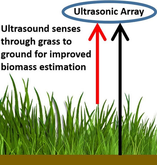
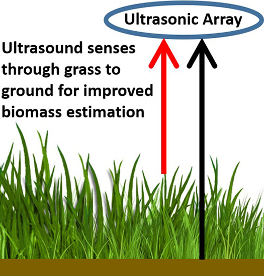
:The profitability of agricultural industries that utilise pasture can be strongly affected by the ability to accurately measure pasture biomass. Pasture height measurement is one technique that has been used to estimate pasture biomass. However, pasture height measurement errors can occur if the sensor is mounted to a farm vehicle that experiences tilting or bouncing. This work describes the development of novel low ultrasonic frequency arrays for pasture biomass estimation. Rather than just measuring the distance to the top of the pasture, as previous ultrasonic studies have done, this hardware is designed to also allow ultrasonic measurements to be made vertically through the pasture to the ground. The hardware was mounted to a farm bike driving over pasture at speeds of up to 20 km/h. The analysed results show the ability of the hardware to measure the ground location through the grass. This allowed pasture height measurement to be independent of tilting and bouncing of the farm vehicle, leading to 20 to 25% improvement in the value obtained for biomass estimation compared with the traditional technique. This corresponded to a reduction in root mean squared error of predicted biomass from about 350 to 270 kg/ha, where the average biomass of the pasture was 1915 kg/ha.
1. Introduction
Accurate estimation of biomass can provide significant improvement in the productivity of agricultural industries that utilise pasture [1]. Biomass may be measured by cutting, drying, and weighing quadrants of pasture. However, this is time-consuming and not a practical option for farmers. An emerging area of research is the use of satellite or areal based remote sensing for biomass estimation [2,3]. However, there is still a need for ground based remote sensing of pastures. There is a range of other technologies that have been used for ground based measurement of pasture biomass, which include optical spectral measurements, capacitance and grass height or compressed grass height measurement [4,5,6,7,8,9].
There has been a range of studies which have used capacitance to measure pasture biomass [5,10]. However, it has been reported that the accuracy of capacitance readings can be affected by moisture due to rain. Optical sensors, such as the GreenSeeker (https://agriculture.trimble.com/product/greenseeker-system/), have also been used to measure a range of parameters of crops and pastures including biomass. These obtain vegetation indices (VI) through calculating the ratio of different spectra of light [11]. Normalised difference vegetation index (NDVI) is the most commonly used vegetation index. While NDVI shows a correlation with biomass, it has been reported that saturation occurs as the biomass increases [8,12,13]. This appears to be related to upper leaves not allowing light to penetrate through the pasture depth. Improved biomass estimation accuracy has been reported when NDVI measurements are used with pasture height measurements [14,15,16,17,18,19]. Modified versions of NDVI have been developed to reduced this saturation effect [13,20].
Pasture biomass is also commonly obtained from measured pasture height, which is the difference between the top of the grass and the ground location. There is a range of techniques that measure pasture height or compressed height by making physical contact with the ground. Examples are manual tape or sward stick (HFRO) height measurements [21], LIDAR [22], rising or falling plate measurements [4,6], and the ultrasonic sward stick [23,24,25]. These techniques require manual measurements and an automated technique that can be used with a farm vehicle is desirable. The C-DAX (http://www.c-dax.co.nz) measures grass height uses a photo diode array mounted in a sled-like structure that is towed over the ground behind a farm vehicle [26]. However, a system that can be mounted directly to a farm vehicle and simultaneously measure both the top of the grass and the ground locations using non-contact (remote sensing) techniques would be desirable.
LIDAR have been mounted to vehicles and used to measure pasture height [27]. This would appear to be able to measure the ground through thin grass. However, there have been reports of LIDAR not detecting ground through more dense pastures [22]. Ultrasonic sensors have also been mounted onto farm vehicles [28]. The height of the grass is then obtained by measuring the distance from the sensor to the top of the grass and assuming that the ground is a set distance from the sensor. However, tilting or bouncing of the vehicle can lead to grass height estimate errors due to the actual ground location not corresponding to the assumed ground location. Schaare describes in a patent an idea of automatically detecting the top of pasture and ground using an ultrasonic sensor [29]. However, no other references has been found in the literature where this technique has been applied for pasture biomass estimation. Reusch used a similar technique for biomass estimation of winter wheat [30]. However, it should be noted that wheat will have much wider spacing between individual plants meaning ground detection using ultrasound is likely to be easier for wheat than for pastures.
Previous work using ultrasound for pasture biomass estimation has only used the first arrival time of the ultrasonic echo from the top of the grass. In reference [31], the authors presented the first study to use ultrasonic echoes from throughout the vertical depth of the pasture to improve biomass estimation by including pasture density information. This was able to be achieved due to novel ultrasonic hardware that was developed for this purpose. The current paper extends the above work by first providing a detailed description of the development of this hardware. It is then shown through farm bike field trials that the hardware can simultaneously detect the top of the pasture and the ground location. To the best of the authors knowledge, this is the first pasture height measurement system that has shown the ability to measure the location of the ground through pasture using non-contact (remote sensing) methods. Also, the hardware developed is the first to use ultrasonic arrays for pasture biomass estimation.
The structure of this work is as follows. The techniques used to design the arrays for pasture profiling are described in Section 2. Section 3 describes the transducer selected to build these arrays. A description of the array hardware developed and the setup for a farm vehicle is then provided in Section 4. Example field trial results investigating the ability of the hardware to detect ground through pasture are then presented in Section 5. Finally the conclusion is given in Section 6.
2. Simulation of Arrays
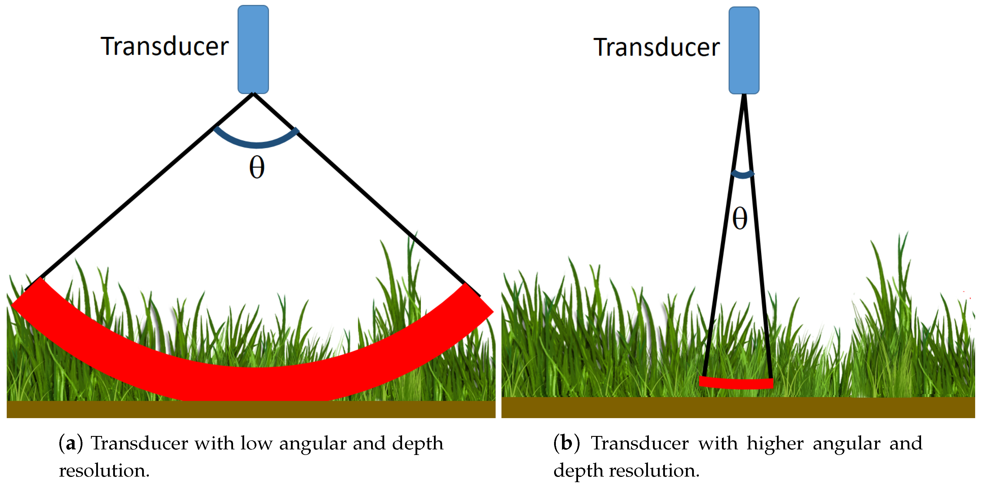
Ultrasound will provide echoes from grass leaves at different layers throughout the pasture depth to the ground. For a given height of the transducer above the ground, reducing the transducer’s angular beamwidth increases the spatial and depth resolution but reduces the sampling area for each ultrasonic pulse, see Figure 1. Also, wider ultrasonic beamwidths may cause errors due to higher segments of grass being detected to the side. To address this, one option could be to move to high ultrasonic frequency (>150 kHz) air coupled transducers, which have a narrower beamwidth and shorter duration pulses. However, this would not be desirable, as higher frequencies would be likely to have poorer ability to penetrate through the grass and obtain echoes from the ground. Frequencies below about 20 kHz are also not desirable because of farm vehicle noise extending into this range. A frequency range of about 20 to 40 kHz, therefore, seemed optimal. However, commercial air coupled ultrasonic transducers, which operate in this frequency range, have poor angular beamwidths and depth resolutions. Ultrasonic phased arrays have been used to reduce the angular beamwidth of ultrasonic transmission. However, ultrasonic arrays have not been used before for pasture biomass estimation.
Most low ultrasonic frequency array studies found in the literature have used commercially available transducers (such as that used for car reversing) for building their arrays. Also, they have generally used tightly packed 2D grid or hexagon layout for transducer array locations. A problem with using these types of dense arrays is that a large number of array elements are required to avoid grating lobes and achieve a desired beamwidth, which is proportional to array diameter. Rather than using dense arrays such as a hexagon or grid array, an alternative is to use sparse arrays such as spiral arrays. These can provide good results for a significantly reduced number of array sensor elements. The arrays developed in this work appear to be the first low ultrasonic frequency (about 20–50 kHz) arrays to have combined both transmission and reception and to have utilised sparse spiral array geometries.
Beam Pattern Properties
The properties of an array may be simulated using beamforming [32]. In the near-field, this beamforming would be a grid of 3D scan points. For far-field beamforming, a grid of scan points may be defined on a hemisphere using spherical polar coordinates. These may be converted to unit vectors in Cartesian coordinates using
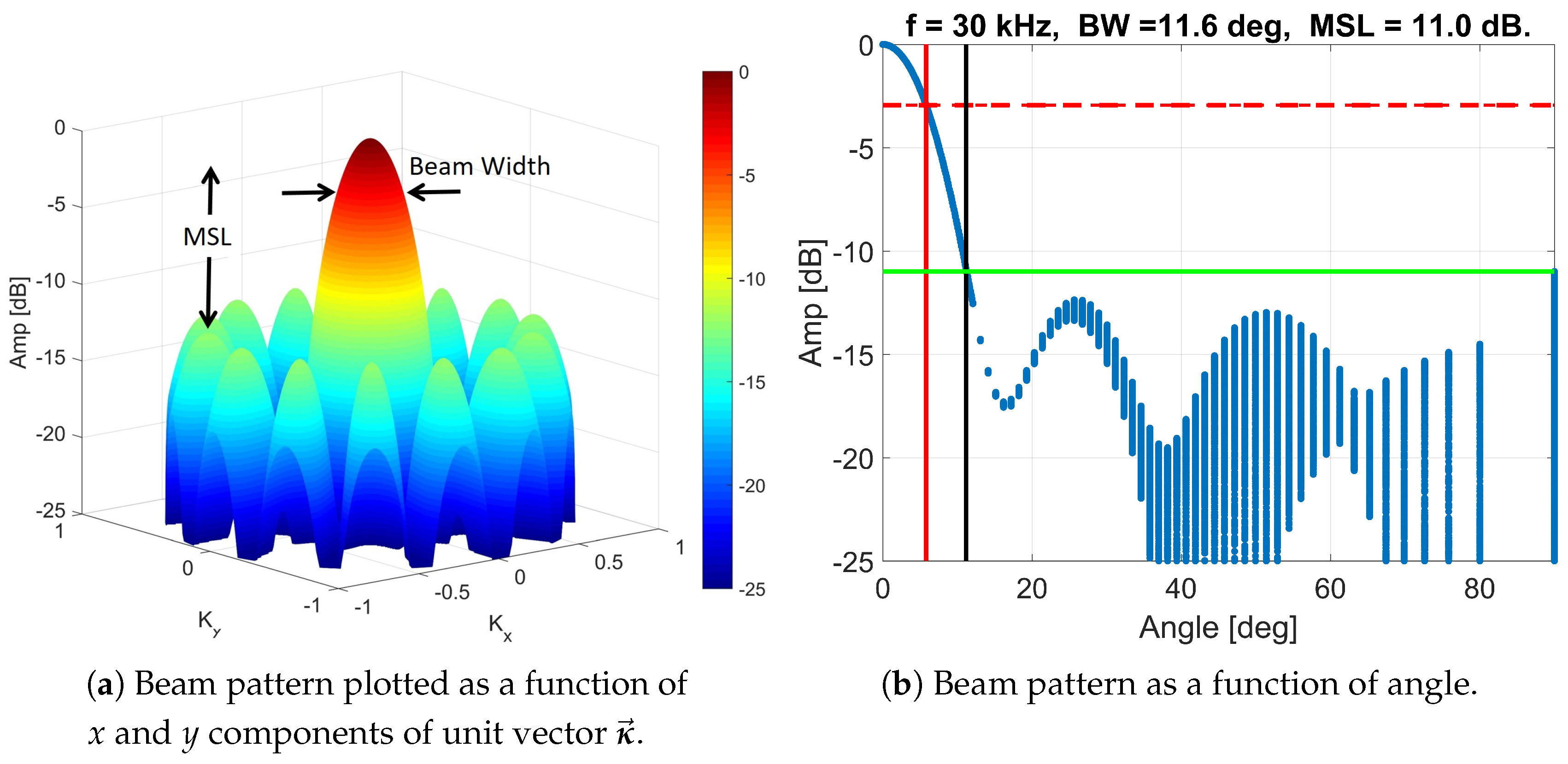
where and are polar coordinate angles. The beamforming map may then be plotted as a function of the x and y components of , as shown in Figure 2. The point spread function for the array is the beamforming map that would occur for a point source located directly in front of the array. Ideally this will be composed of a single main lobe with side lobes, see Figure 2.
The angular resolution of an array is given by the beamwidth (BW) of the array, which is the width of the main lobe at −3 dB down from the peak. In the near-field, the beamwidth is usually given as a distance while in far-field it is expressed as an angle. The beamwidth of an array may be approximated using
where z is the distance from the array, is the wavelength of the ultrasound, and D is the diameter of the array. The dynamic range of the array may be defined as the difference in dB from the peak of the main lobe to the peak of the highest side lobe. This is referred to as the maximum side lobe level (MSL). This is related to the number and placement of ultrasonic sensors in the array. Note that to convert the amplitude MSL (used in this work) into an intensity MSL (traditionally used for microphone array literature), one should double the amplitude MSL value. For example, an amplitude MSL of 10 dB is equivalent to an intensity MSL of 20 dB. The BW values will also be different when compared with those measured using intensity.
Instead of just having a single main lobe, multiple main-lobes referred to as grating lobes can occur. These are undesirable for imaging applications as they result in sound being transmitted/received in multiple directions. These occur as a result of spatial aliasing caused by the minimum spacing between array elements being greater than half of the wavelength. If the ultrasonic sensors have a gain that varies with angle, the side lobes and any grating lobes may be attenuated compared with what would be expected for omnidirectional sensors.
3. Transducer Selection
There are a range of characteristics that should be considered when choosing a transducer. These include the transducer’s frequency response, transient response, and directivity pattern. To evaluate which transducer was the best choice, a range of commercially available transducers were purchased for evaluation.
3.1. Transducer Characteristics
The desired frequency of transmission was a factor when choosing the transducer for this work. High ultrasonic frequencies were not used as it was believed these would provide poor penetration of the signal through the pasture. Similarly, frequencies below about 20 kHz are also not seen as desirable because of farm vehicle noise extending into this range. Figure 3 shows an example measurement of farm bike noise made with a broad band microphone. A transducer which could operate in the frequency range of about 20 to 40 kHz, therefore, seemed optimal.
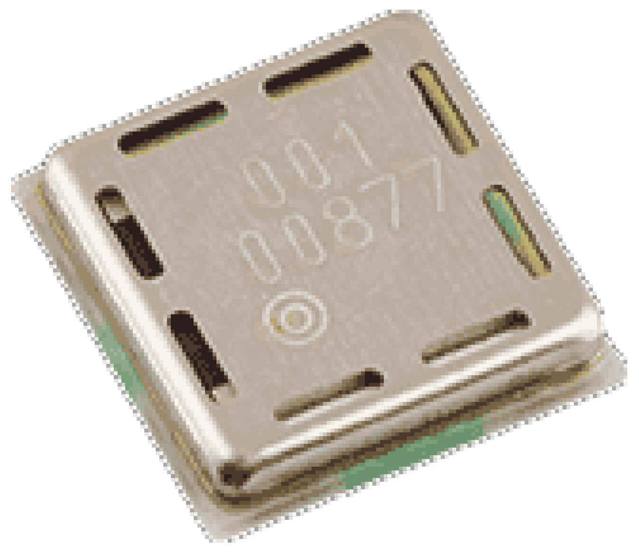
One of the transducers identified as being suitable was the Murata MA40H1S-R surface mount transducer, shown in Figure 4, which operated at 40 kHz. No other works have been found where this transducer has been used for arrays apart from those using a few transducers [33]. (Manufacture of this transducer appears to have been stopped since this work started.)
3.2. Transducer Transient Response
Transducer ringing is the tendency of a transducer to oscillate (usually at its resonance frequency) after the excitation signal had stopped. Most low ultrasonic air coupled transducers are designed for measuring the distance to an object (e.g., a car reversing transducer). In this case, one is only interested in the first arrival time of the ultrasonic echo. Increased sensitivity of the transducer at its operating frequency is beneficial as it increases the echo strength, even though this increases ringing. However, for the application of profiling down through pasture, ringing is an issue as it reduces depth resolution.
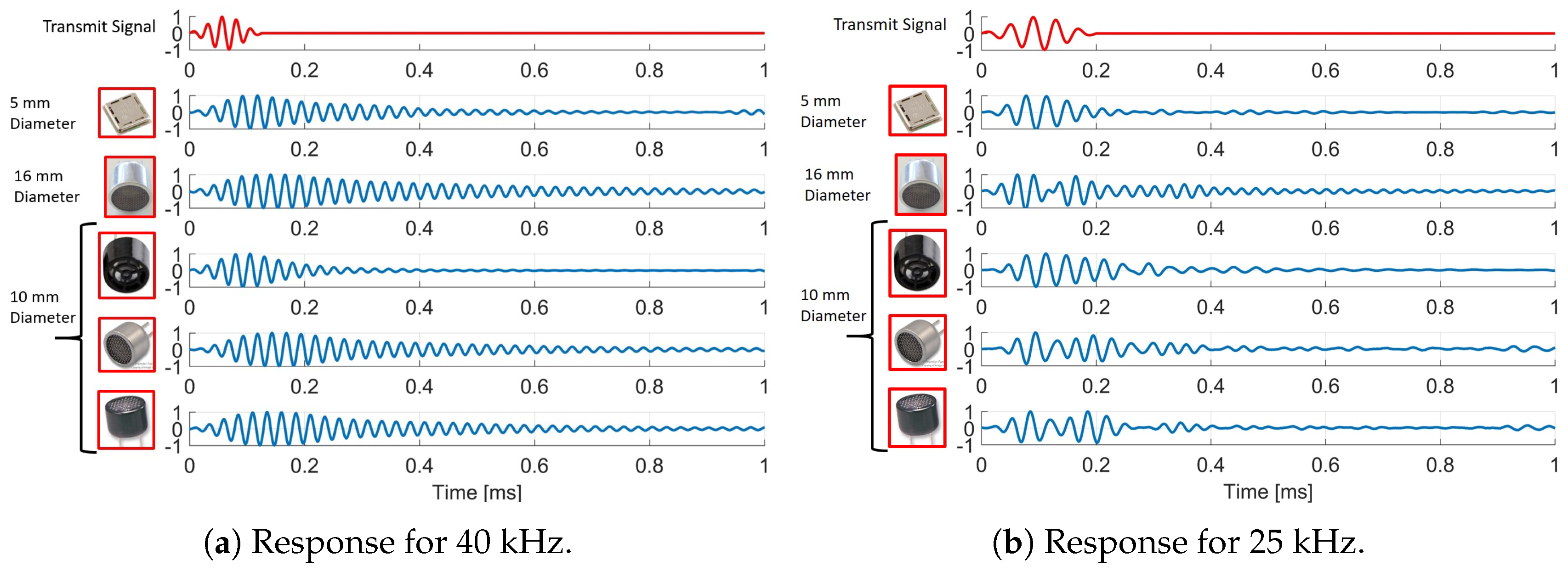
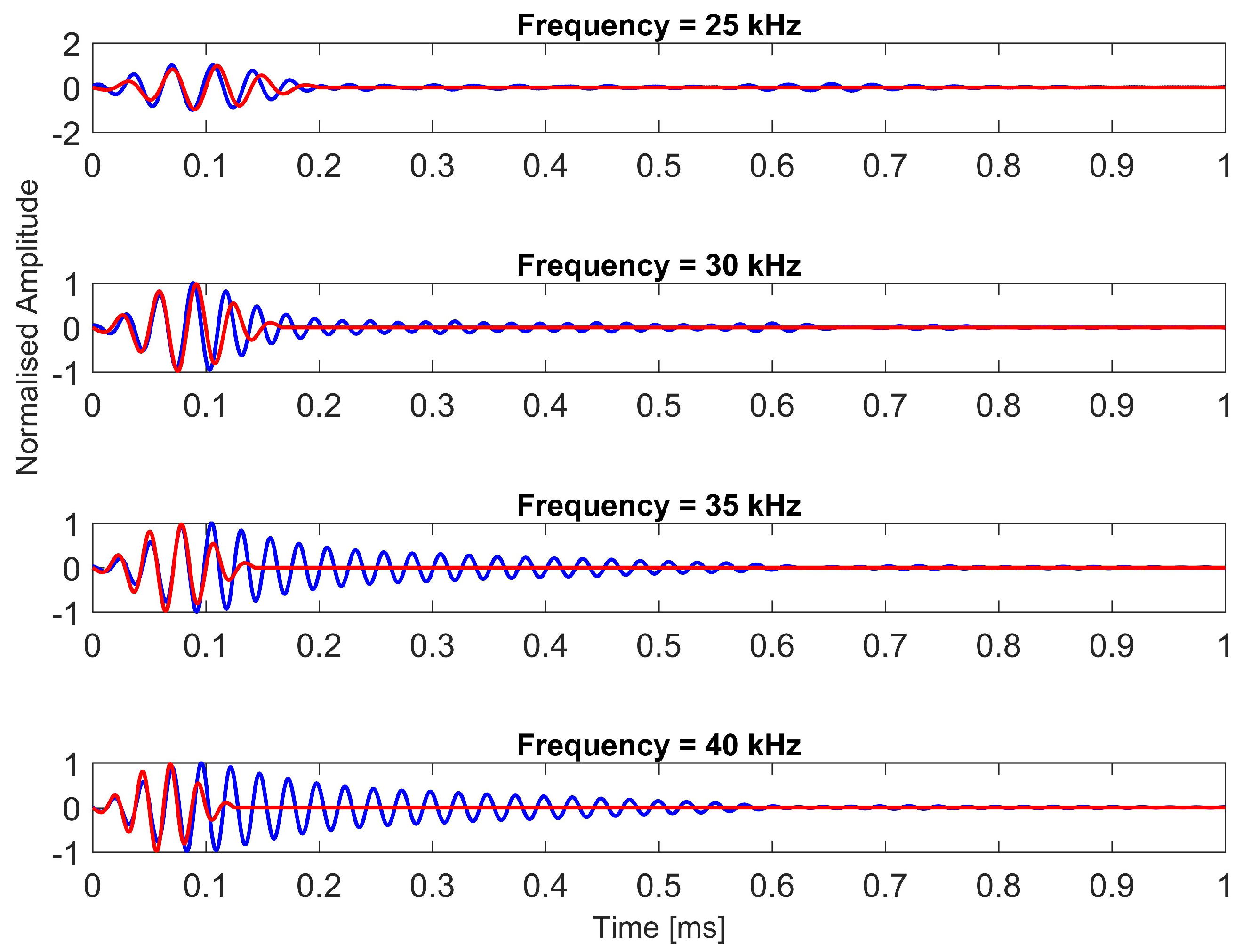
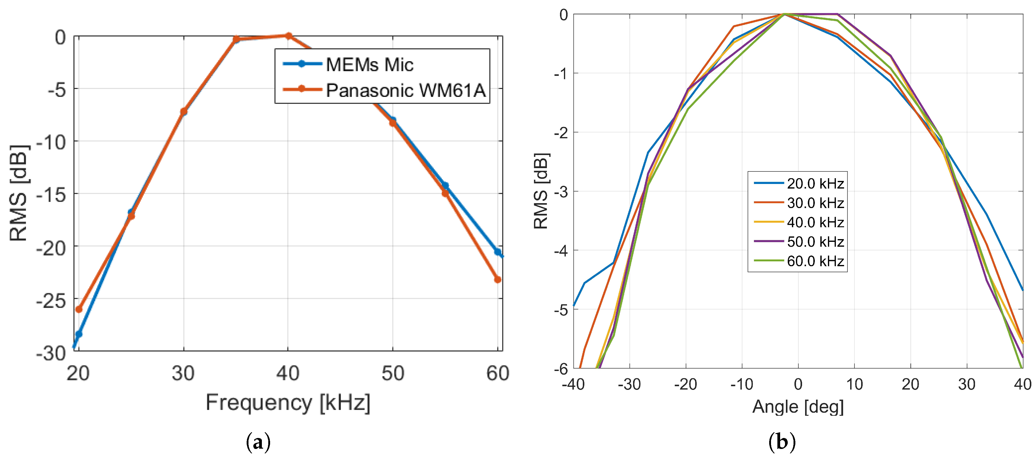
Measurements were made to investigate the ringing of a range of transducers. Figure 5 shows examples of the received signal measured by a microphone (Panasonic WM61A with preamplifier) when transducers were excited by 5 cycles of a Hamming windowed sine wave. The Murata MA40H1S-R surface mount transducer exhibits comparatively low ringing compared with the other transducers investigated. Figure 6 shows its response for several transmit frequencies from 25 to 40 kHz. The ringing reduces as the transmit frequency moves away from the resonant frequency (40 kHz). However, this comes at the cost of reduced gain, see Figure 7a. The measured variation of gain of the transducer with angle is shown in Figure 7b.
Tests were also made using the MA40H1S-R transducer for both transmission and reception. However, it was found that the gain was lower and ringing was increased compared with using a microphone for reception. Ringing was occurring on the transducer for both transmission and reception. Based on these results and the size of the transducer, it was decided to use the Murata MA40H1S-R transducer for transmission but use a MEMs microphone for reception. This MEMS microphone can be used for ultrasonic frequencies and its measurement of the frequency response of the transducer is similar to the WM61A microphone, see Figure 7a. It is a surface mount component and uses a hole through the printed circuit board (PCB) to detect the sound. Since the MA40H1S-R transducer and the MEMS microphone were on opposite sides of the PCB, they can be closely spaced. This information was able to be fed back into the array design simulations described in Section 2.
4. Array Hardware Developed
Two main hardware versions were developed for investigating ultrasonic pasture biomass measurement. These are described here as “Version 1” (V1) and “Version 2” (V2). The V1 hardware had a fixed beamwidth and was the main tool to be used for field trials. The V2 hardware was developed to investigate the effect of using different beamwidths and numbers of transducers and microphones. It was a research tool and not viewed as a potential commercial product.
These array boards were designed using simulations with the process described in Section 2. Rather than using a dense array design, a sparse array design based on the multi-arm spiral array was used. This type of array design allows significantly fewer array elements to be used compared with a dense array like a grid, while maintaining good MSL values over a wide frequency range. An iterative approach was used to optimise the array design for a desired MSL, beamwidth and number of microphones and transducers. Key parameters of these two hardware versions are given in Table 1.
4.1. Version 1 Array
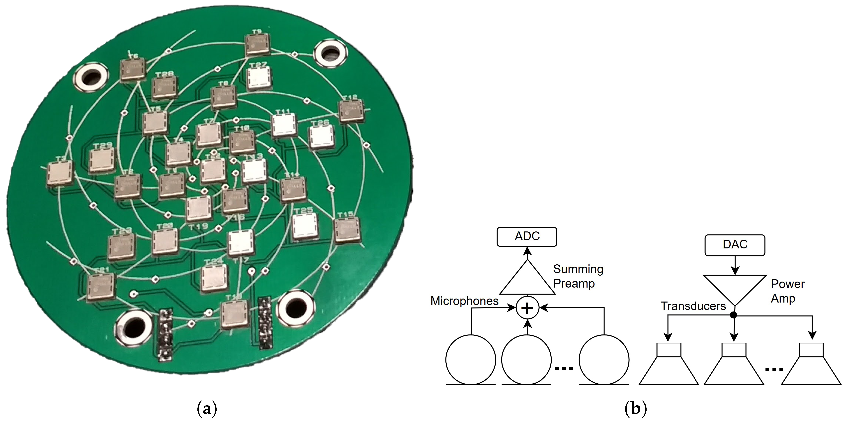
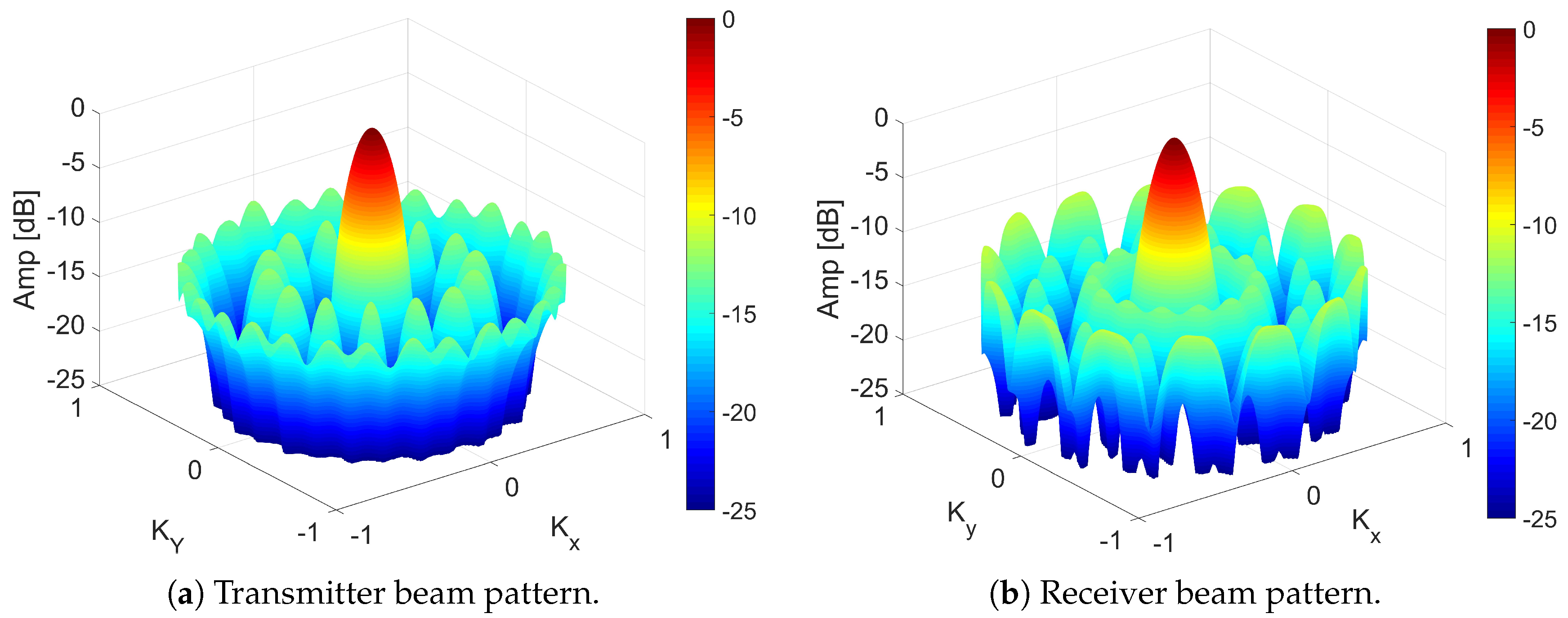
The Version 1 (V1) ultrasonic array PCB is shown in Figure 8a. The surface mount transducers were placed onto the front side (facing the pasture) of the PCB. They were all wired in parallel and driven by a single amplifier and a DAC channel of a Data Translation DT9836-12-2-BNC board, see Figure 8b. The MEMS microphones were positioned on the back side of the board and the ultrasonic signal was sampled through holes in the PCB. The signals from the microphones were summed into a single channel using a summing pre-amplifier/filter circuit and connected to a single ADC channel of the DT9836 board. This meant that the array was directed in a single direction (perpendicular to the array) and was equivalent to a transducer with a directivity pattern given by the point spread function of the array. Examples of the simulated amplitude beam pattern (point spread function) for transmit and receive at 30 kHz are shown in Figure 9.
4.2. Version 2 Hardware—High Resolution Array
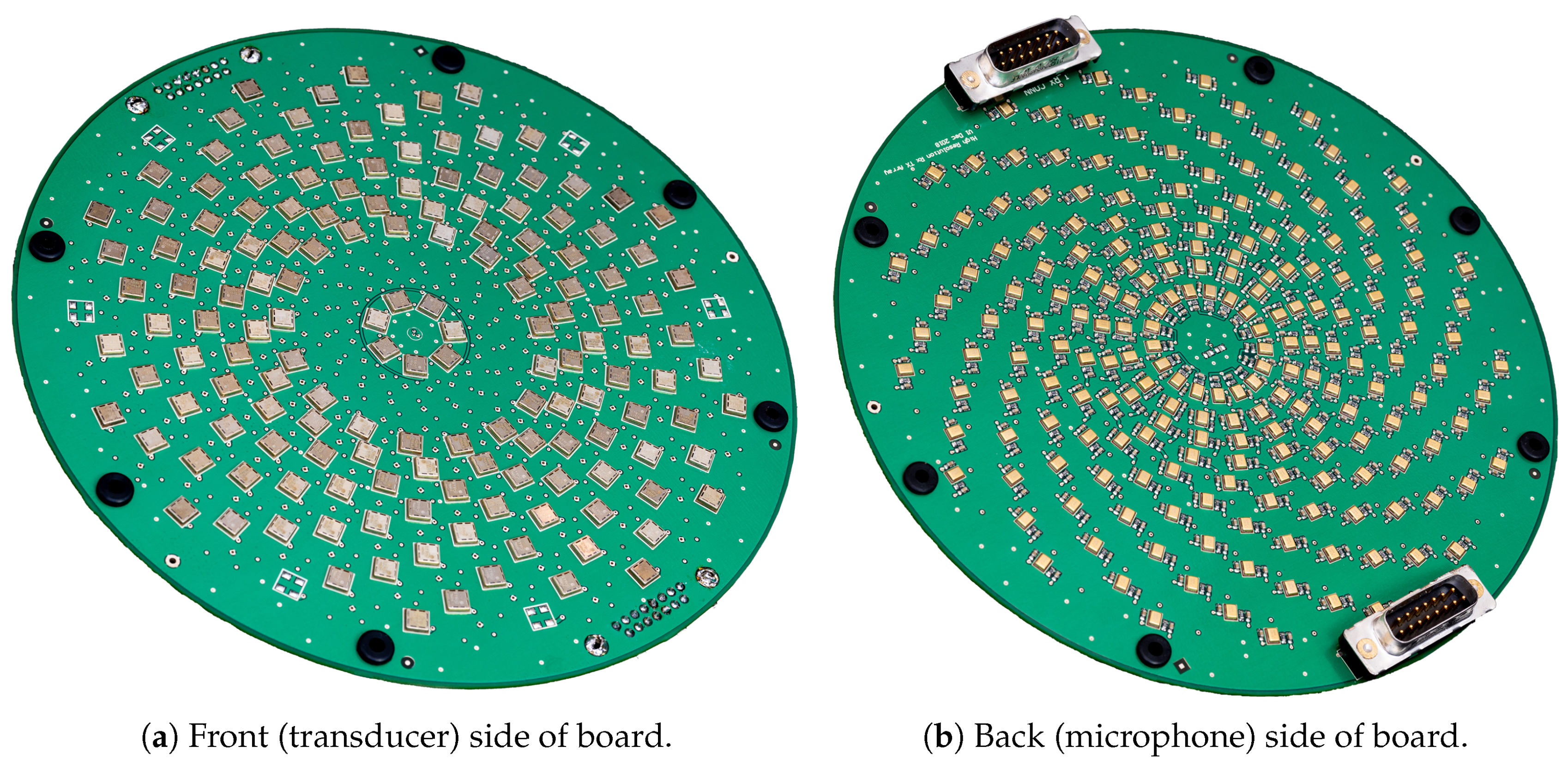
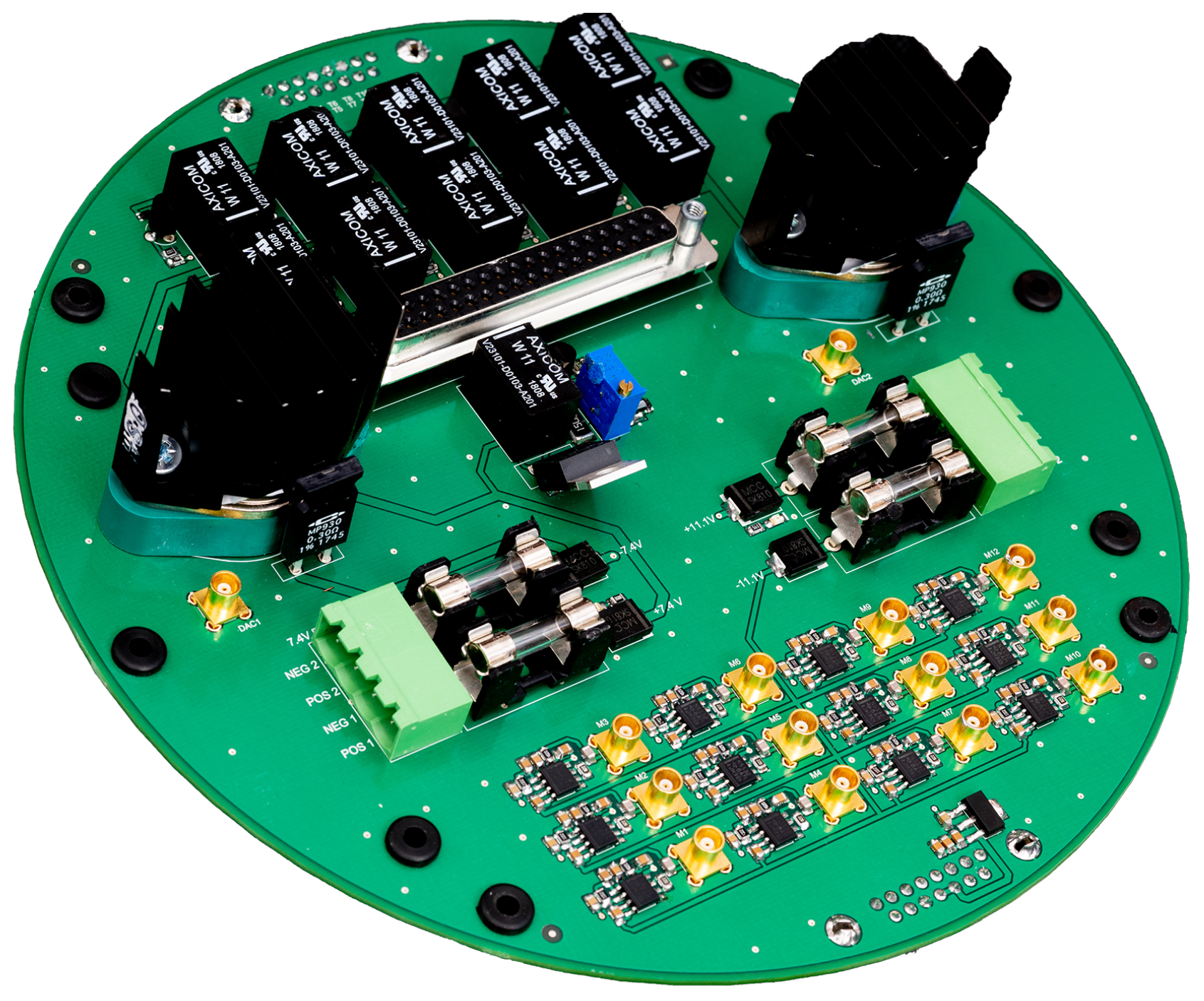
The Version 2 array PCB board is shown in Figure 10. This array was designed for 160 Murata MA40H1S-R surface mount ultrasonic transducers (six of these were not populated) and 204 MEMS microphones. With associated components (SMD resistors and capacitors), there were about 1000 components to be positioned on a 180 mm diameter PCB. Accurate localisation of all component was required as this determined the array geometry. Manual placement of all these components would have been difficult. Therefore, a technique was developed that automated the positioning and orientation of all components and via points using Matlab and Altium Designer. The array PCB board plugged into another PCB containing amplifiers, relays and connections to the ADC and DAC channels, see Figure 11.
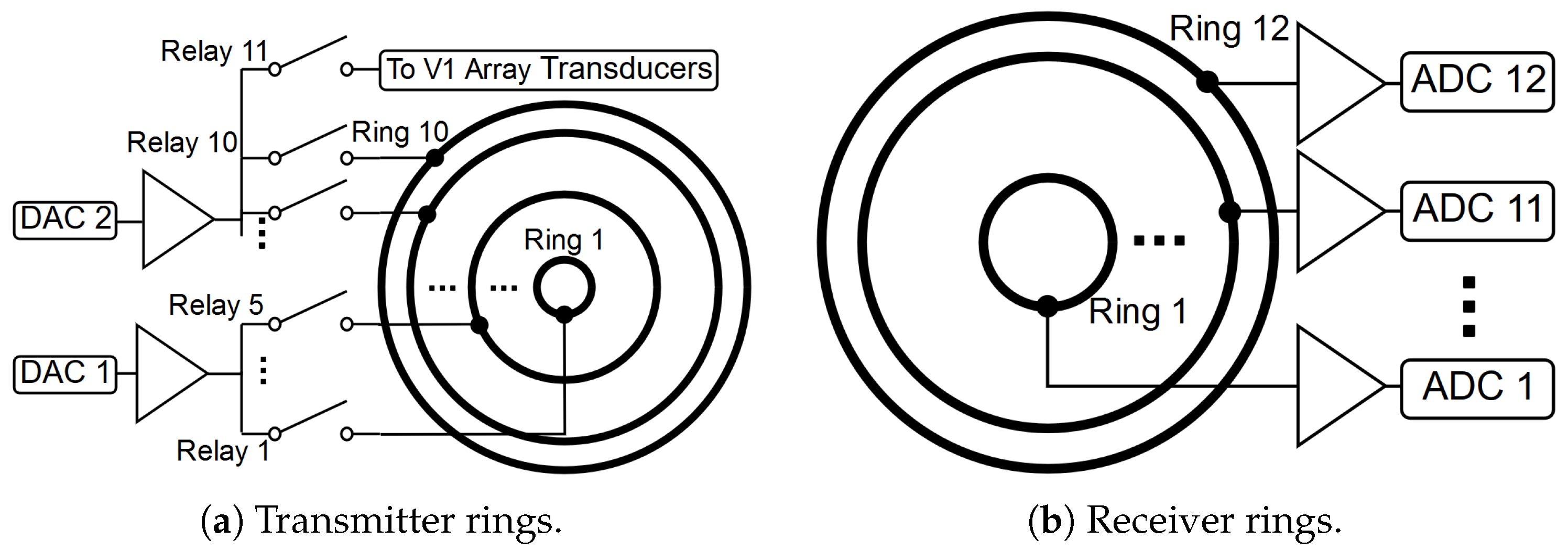
The V2 board’s transmit and receiver arrays were both based on a 17 arm multi-arm spiral. The receiver array contains 12 rings each containing 17 microphones. For each of these rings, the signal from all the microphones in a ring are combined using a summing preamplifier and the output passed to one of the 12 ADC channels of a Data Translation DT9836-12-2-BNC board. Similarly, there are 9 transmitter rings each containing 17 transducers plus an inner transmitter ring of seven transducers. The transducers in each ring are wired in parallel and driven through a relay by one of two power amplifier/DAC channels of the DT9836 board. The relays were controlled by the digital outputs of the DT9836 board, refer to Figure 12 for a diagram of this configuration. An additional relay was added to allow the output of one of the power amplifiers to also drive the V1 board transducer array.
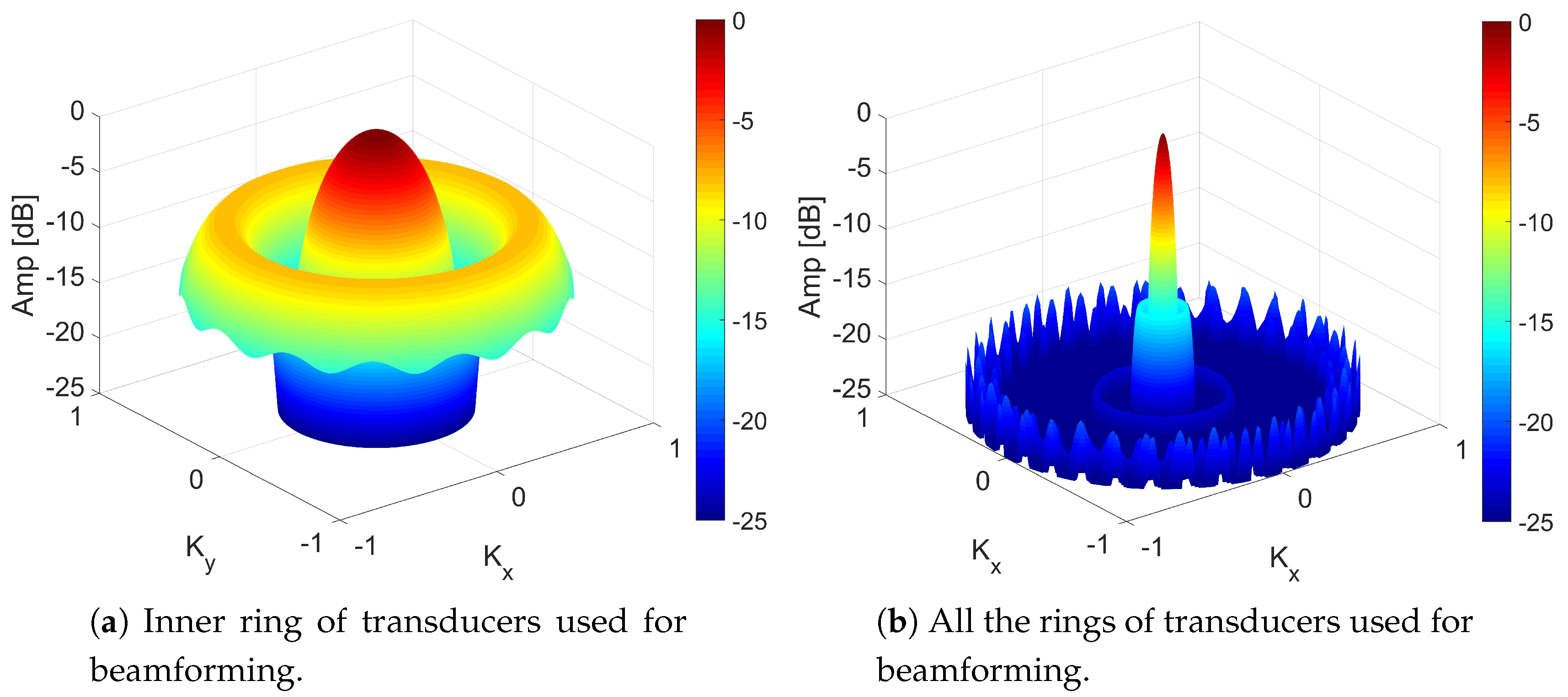
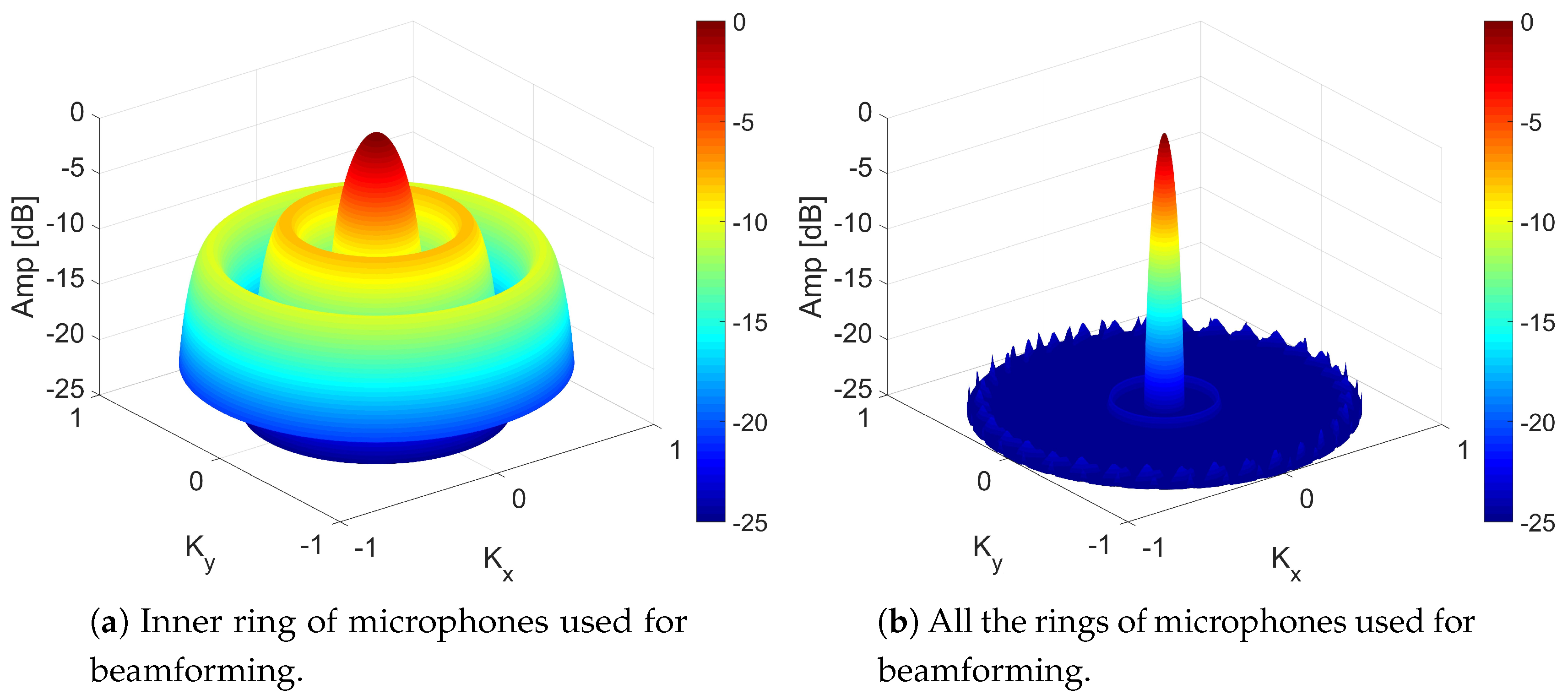
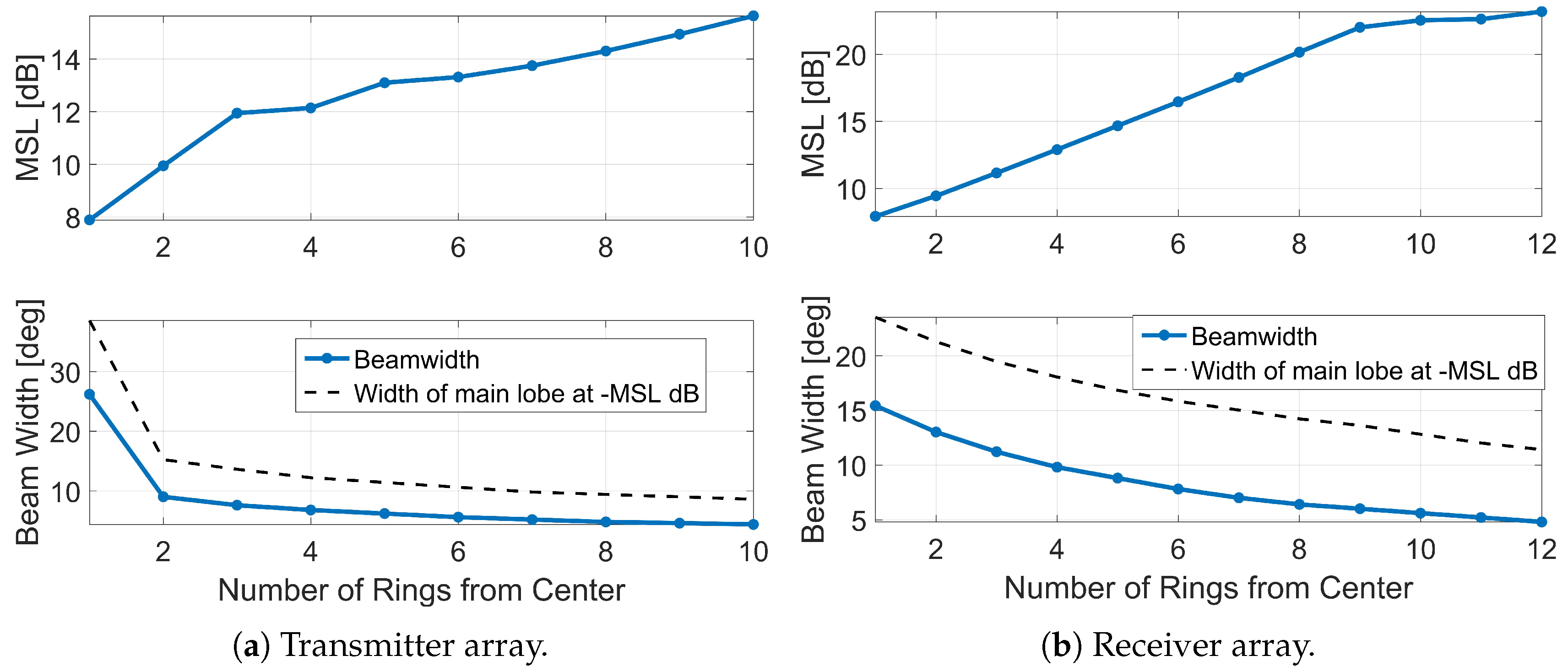
This design of multiple independent transducer and microphone rings was done to allow the beamwidth of the array to be adjusted. From Equation (2), we know that the array beamwidth is dependant on the diameter of the array. Therefore, if all the rings are used for transmission/reception, then a high angular resolution (narrow beamwidth) would be obtained. As the number of rings used for transmission/reception is reduced (from the outside towards the center), the effective diameter of the array reduces causing the angular resolution to reduce (increased beamwidth). In addition, one would expect that the dynamic range (MSL value) would also reduce. Note that the beamwidth of the reception can be adjusted during post processing by summing different ADC recorded channels. Examples of the simulated beamwidths for the V2 array are shown in Figure 13 and Figure 14. The variation in simulated beamwidth and MSL values as a function of rings used are plotted in Figure 15. One factor to keep in mind is that, as the number of transmit/receive rings is decreased, the acoustic power will also decrease as fewer sensors are being used.
4.3. Mounting of V1 and V2 Arrays
There was concern that noise could be an issue in field trials when the arrays were operated from a farm bike. This was taken into account in the final mounting system used for farm bike trials, see Figure 16a. The V1 array was mounted directly to the aluminium support structure that was to be attached to the front of the farm bike. It was believed that vibrations generated by the farm bike would not be an issue since these would have frequencies below the ultrasonic frequency range. However, to check that this was the case, vibration dampening fittings were used to mount the V2 array’s PCBs to its metal enclosure and additionally to mount this enclosure to the support structure that would be attached to the farm bike. In addition, more rigorous electrical shielding was used for the V2 array (fully encased in a metal enclosure with an acoustically transparent wire mesh over the front of the array, etc) compared with the V1 array. Both the arrays and the data acquisition units were operated using LiPo batteries, rather than using the farm bike’s battery, to reduce the chance of electrical noise being an issue. These arrays were controlled using two data translation DT9836-12-2-BNC boards, which were mounted to the main support arm. These were operated using a transmit sampling rate of 500 kSPS, a receive sampling rate of 225 kSPS and a resolution of 16 bits. Software was written using Matlab for both data acquiring and post processing.
Initial field trials were performed and both arrays appeared to have good signal to noise ratios indicating that the extra steps described above to reduce noise in the V2 array was not needed. Hence, the mounting system for the V1 array was not changed. Acoustic noise from the farm bike did not appear to be an issue. However, acoustic foam baffles were added around both arrays to eliminate small echoes from the farm bike observed in the raw data. A temperature sensor and an IR proximity sensor were also added for, respectively, temperature-dependant speed of sound calculations and localisation of measurements made during the field trials (discussed further in Section 5).
4.4. Experimental Measurement of Beam Patterns
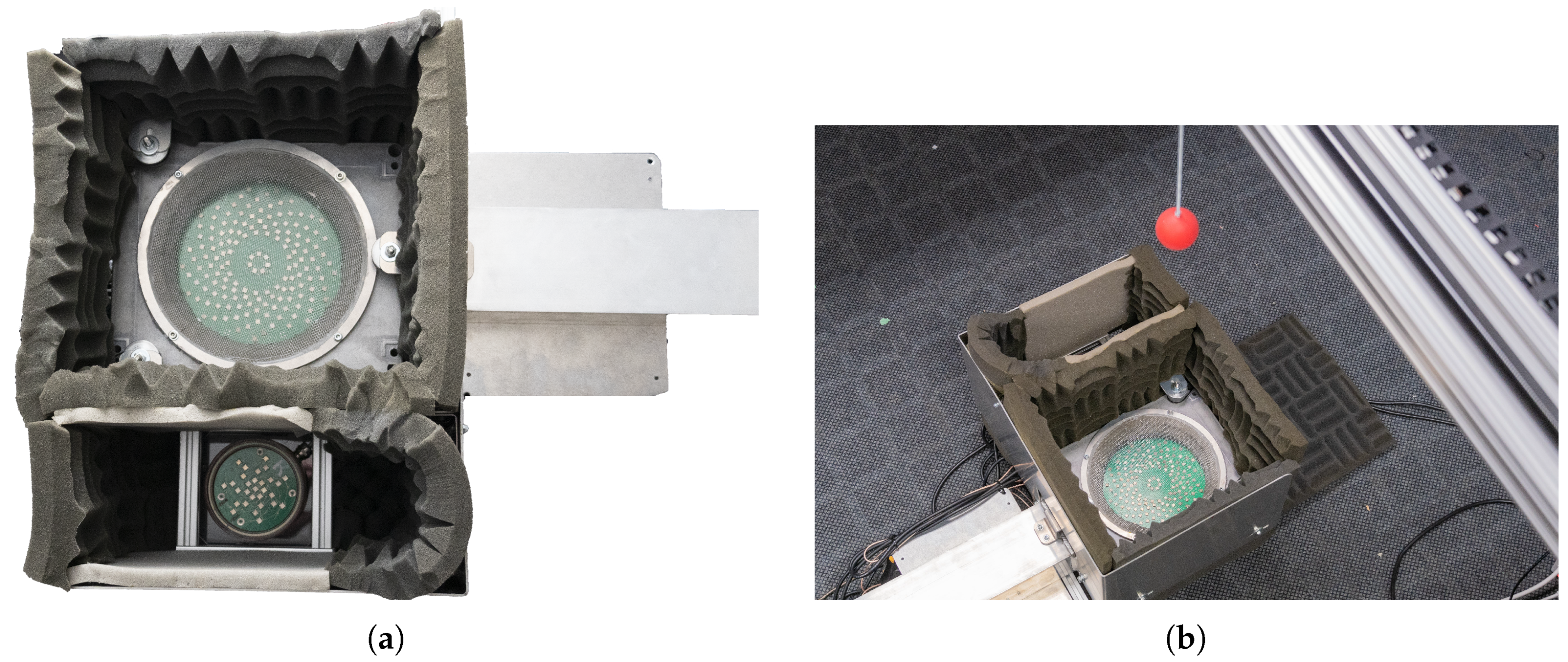
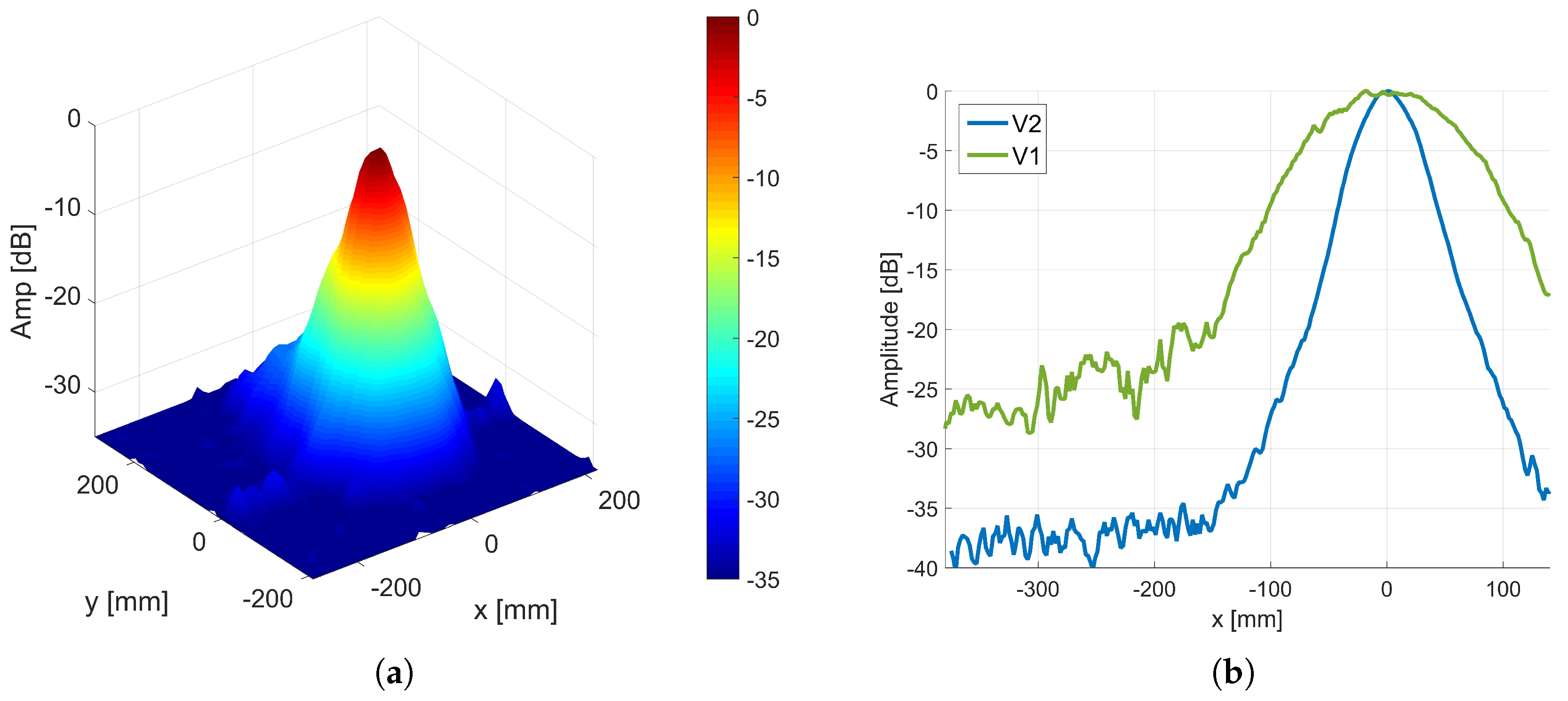
Experimental measurements were made of the combined transmit and receive beam patterns the V1 and V2 array, when they were mounted into the enclosure shown in Figure 16a. The array hardware was placed on the ground facing upwards. A 40 mm sphere (a table tennis ball) was mounted about 805 mm above the array with a thin rod to a 2D gantry motion platform, see Figure 16b. At each location of the sphere, an ultrasonic pulse was transmitted and the root mean square (RMS) of the resulting echo was obtained. By repeating this process for a 1D line of points or a 2D grid of point, the beam pattern of the arrays were able to be generated. Figure 17a shows an example of the measured 2D beam pattern for the V2 array using all the transducer and microphones in the array for a Hann windowed, five-cycle, 30 kHz sine wave pulse. There is a slight non-uniformity to the beam pattern below about 25 dB down from the peak. This appears to be related to the shape of the acoustic foam shielding around the ultrasonic array. Corresponding 1D beam pattern plots for V1 and V2 arrays are shown in Figure 17b.
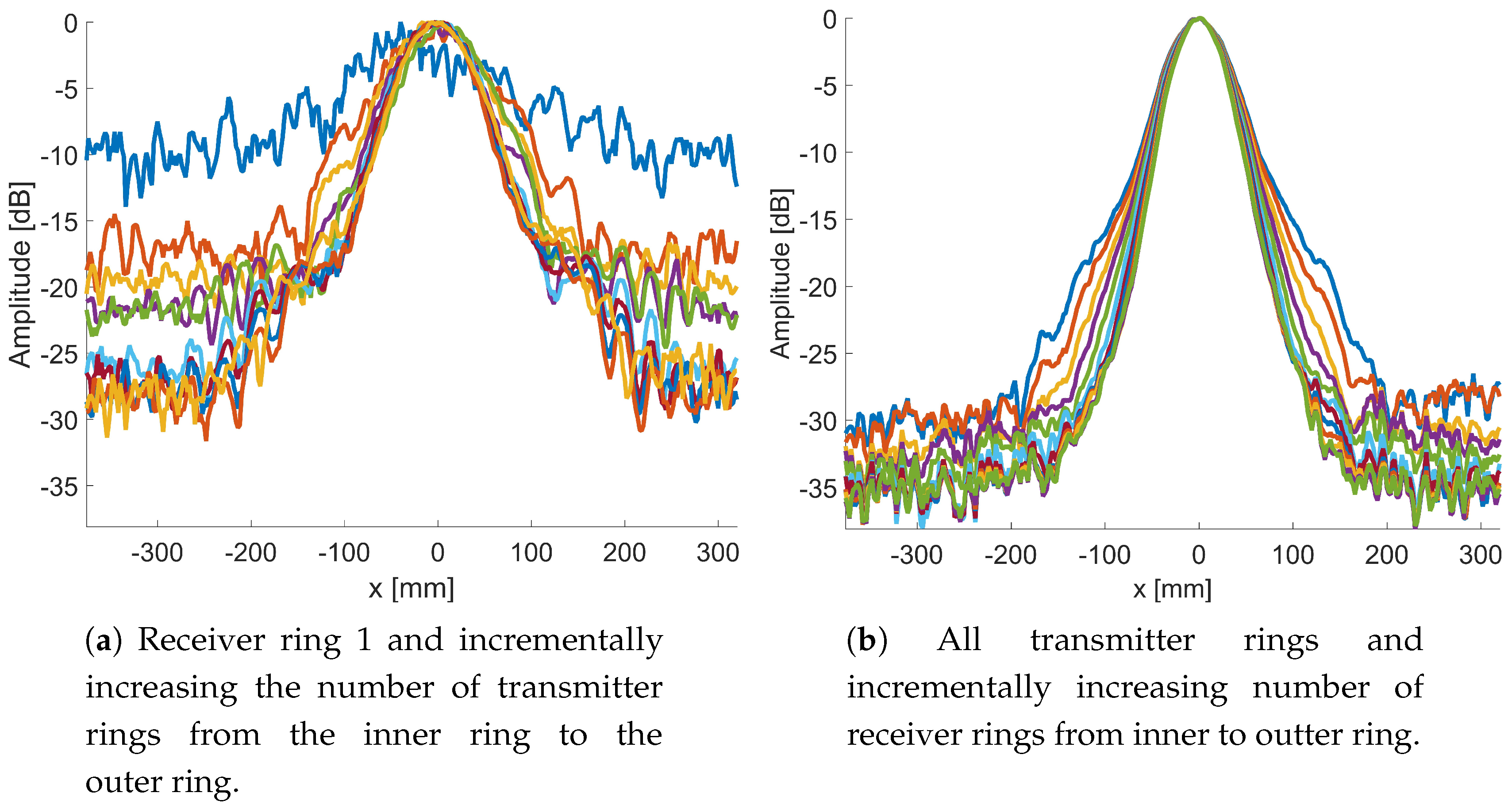
Figure 18 shows examples of the measured 1D beam patterns for the V2 array for a 0.5 ms duration linear chirp from 20 to 35 kHz. These show how the beamwidth reduces and the MLS increases as the diameter of the array and number of sensors increase. Examples of the measured beamwidths and MLS values are given in Table 2 for the V1 and different configurations of microphone and transducer rings of the V2 array.
The V1 array has a fixed beamwidth (8.7°) and MLS (25 dB). The V2 array can be used to investigate if a narrower beamwidth (down to 3.3°) and higher MLS (up to 33 dB) compared to the V1 gives any improvement of biomass estimation.
5. Example Field Trial Results
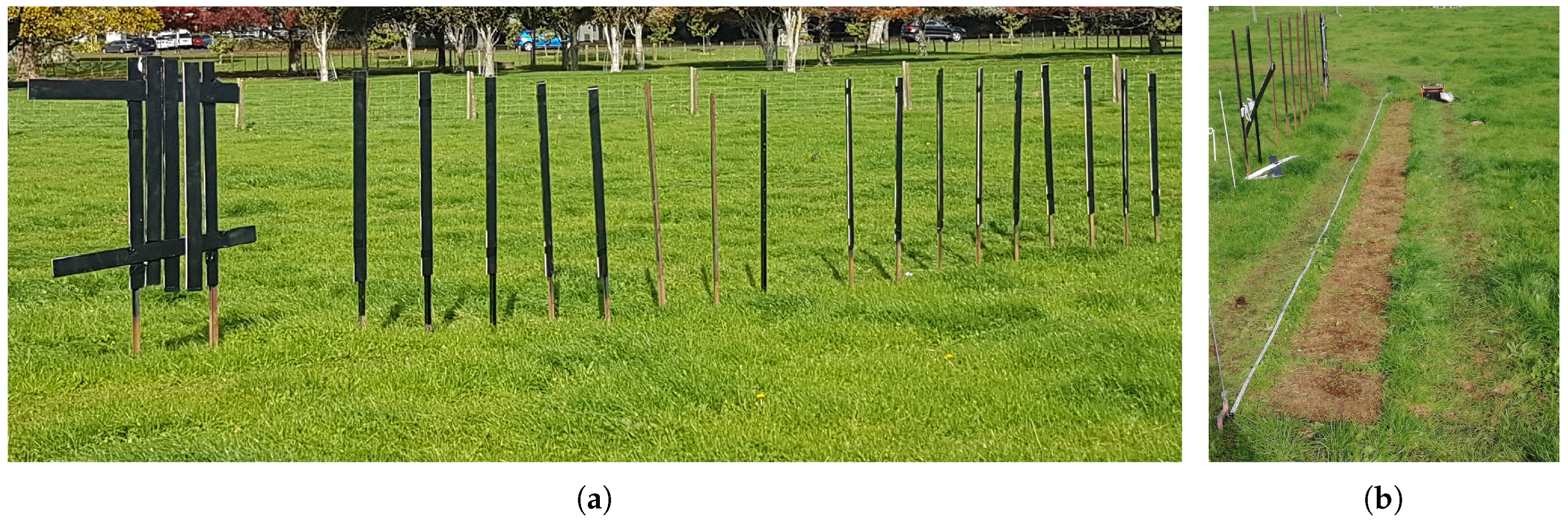
Field trials were performed to see how the hardware performed when operated from a moving vehicle over pasture. The field trials were performed at AgResearch in Ruakura, Hamilton, New Zealand in May (autumn) 2019. The pasture was predominantly comprised (>80%) of perennial ryegrass (Lolium perenne), with the remainder mostly white clover (Trifolium repens), buttercup (Ranunculus repens) and plantain (Plantago lanceolata). Figure 19 shows the V1 and V2 arrays mounted to a farm bike for field trials. The arrays were positioned side-by-side (as shown in Figure 16a) and were about 1015 mm above the ground. Measurements were made over three transects. Field trial results are provided in this work are for “Transect 2” shown in Figure 20. This transect had a slight slope in the ground near the start which flattened off near the middle. Ultrasonic measurements for both the V1 and V2 arrays were made over this transect at bike speeds of roughly 5, 10, 15, and 20 km/h. Care was taken by the driver to keep to the same tire tracks for each pass. The grass was then cut to ground using twenty 0.5 × 0.5 meter quadrants, see Figure 20b. Ultrasonic measurements were then repeated using the farm vehicle over the bare earth. AgResearch then washed and dried the cut grass for each quadrant using a temperature of about 65 °C for 24 h. These samples were then weighed to obtain biomass measurements.
Ultrasonic measurements performed from a moving farm vehicle was significantly more challenging compared with that for stationary measurements. The farm bike bounced around and experienced tilting as it moved over uneven pasture. Also, it was difficult to make comparisons with cut and weigh measurements due not knowing the position of the bike when a given ultrasonic measurement was made. A system was needed which allowed one to know where the bike was when an ultrasonic transmission occurred. This system needed to be synchronised with the ultrasonic system and be safe for the farm bike driver (non-contact) and not affect the ultrasonic measurements.
5.1. Horizontal Position Measurement using IR Sensors
A rang of options were evaluated for measuring the horizontal position of the farm bike when ultrasonic pulses were transmitted. A differential GPS system was considered but it was decided that it would be difficult to achieve the desired accuracy of about 0.1 m. Instead an IR sensor system was used which detected black painted cards attached to poles at known locations along the transect, see Figure 20. The ultrasonic transmit and received signal and the IR sensor output were recorded simultaneously for the duration of each pass of the farm bike over a transect. Transmissions were repeated every 50 ms. The position x where a transmission occurred was estimated using
where is the mean speed measured using least squares fitting and t is the time after the particular IR reflector is passed and is the horizontal position of this reflector card. This IR system appeared to provide the required position accuracy but was somewhat challenging to use due to variability of sunlight causing some IR reflectors to be missed and requiring the gain to be adjusted.
5.2. Improved Grass Height Measurements
5.2.1. New Height Measurement Technique
Traditionally grass height estimation from moving vehicles is obtained from ultrasonic sensors by measuring the distance from the sensor to top of the grass and assuming the ground is a set distance below the sensor. The grass height is then calculated using
A problem with this method is that bouncing of the farm vehicle and tilting of the farm vehicle can mean that the assumed distance to ground is not correct resulting in inaccurate grass height estimation. This error could be eliminated if the actual distance from the sensor to the ground was known. In this case, the grass height is
The ultrasonic arrays presented in this work were designed with the aim of being able to obtain echoes vertically through the grass to the ground. It was anticipated that this might allow the location of the ground to be detected through grass.
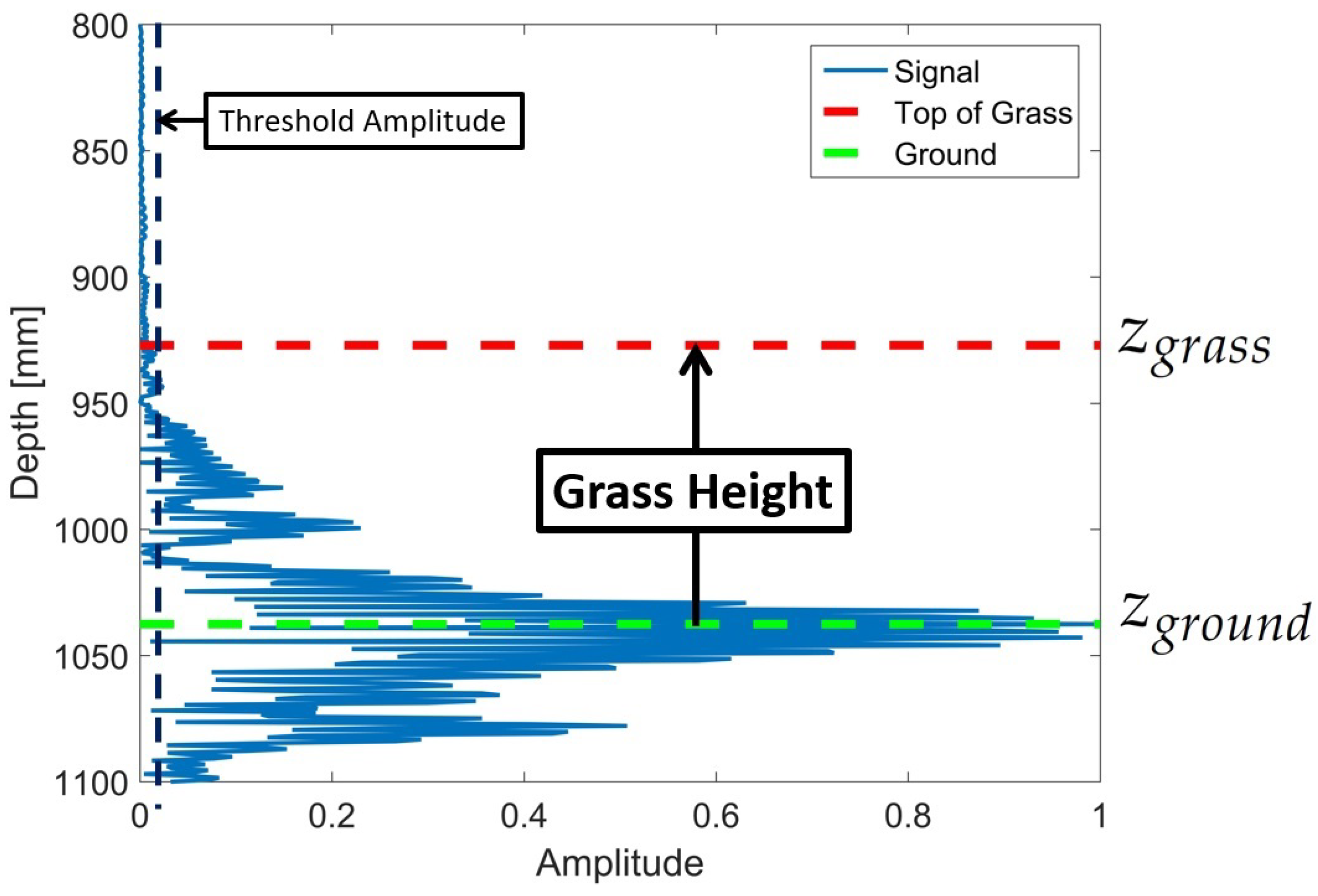
Depth measurements were made by transmitting a 20–35 kHz linear chirp with a duration of 0.5 ms. Cross-correlation of the resulting received echo signal with the transmit signal was then used to increase the temporal resolution. An example of the resulting processed signal is shown in Figure 21 for measurements made with the bike driving over pasture. The top of the grass (shown as a red dashed line in Figure 21) was assumed to be when the signal first goes over a threshold. The ground (shown as a green dashed line in Figure 21) was assumed to be the peak in the cross-correlated signal. In practice, however, often the highest peak did not correspond to the ground but the grass above. To address this, the ground was instead assumed to be the highest peak within a distance range, which was centred near where the ground was expected to be located (about 1015 mm from the array).
5.2.2. Evaluation of Height Measurement Techniques
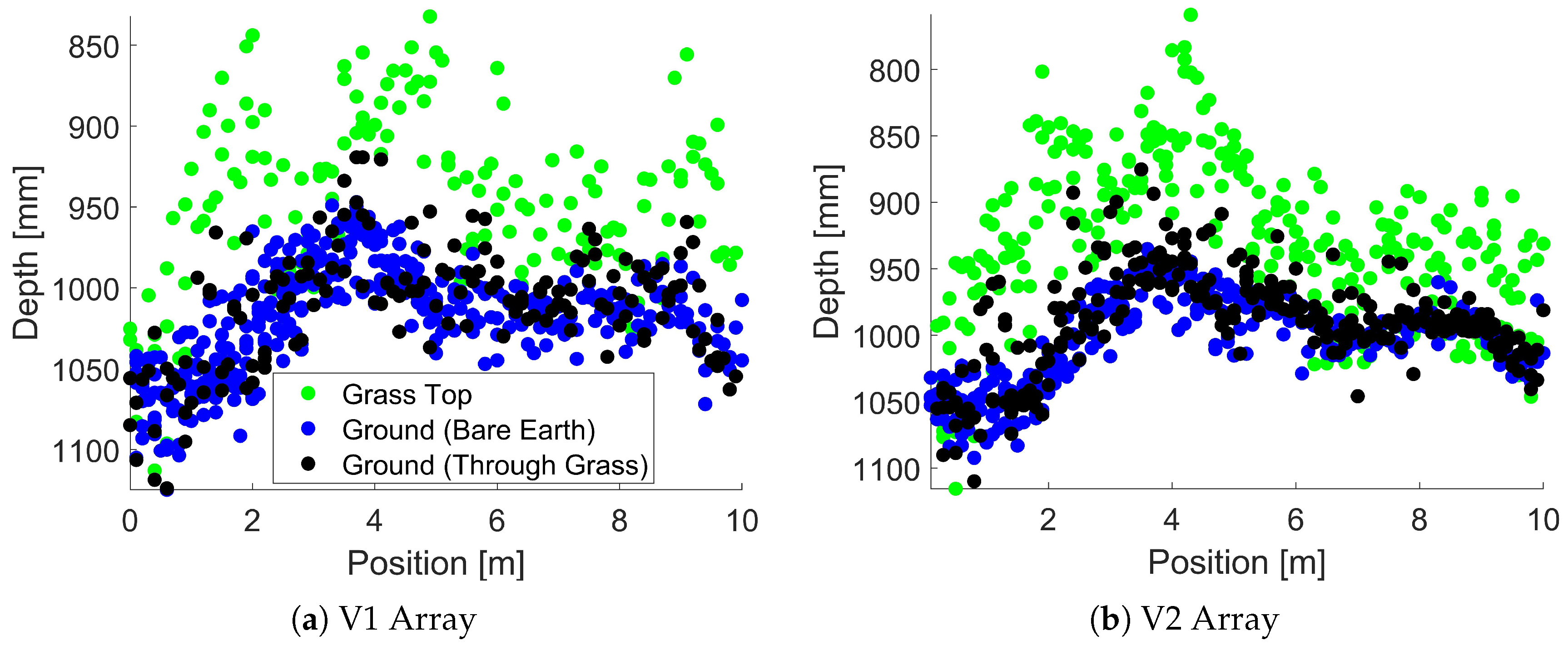
Bike trial measurements had been made for “Transect 2” for speeds of about 5, 10, 15 and 20 km/h with grass and then again after the grass had been cut to ground. The distance to the top of the grass () and ground location () was calculated for the measurements made with grass. The ground location () was then also obtained for the bare ground measurements using the same technique as that used for grass measurements. Figure 22 shows the resulting measured distances of the array from the top of the grass and to the ground. Within each half meter quadrant, there is roughly about 50 mm variation in both measurements of the ground distance. This would be expected given the bouncing of the bike and some uncertainty in horizontal distance. However, Figure 22 also shows about 10% of the ground measurements made through grass appear to be located too high (within the grass) compared with that for bare earth measurements. This appears to be due to the highest peak in the signal for these data points being from the grass rather than at the surface of the ground.
There is also a significant variation in the average measured ground level over the transect for measurements made both through grass and with bare ground. This variation is proportional to the grass height and is due to a slight slope of the ground which was amplified by the fact that the arrays were mounted a distance in front of the farm bike. This variation in distance of the array from the ground would be expected to lead to errors in the measured grass height using the traditional technique given in Equation (4).
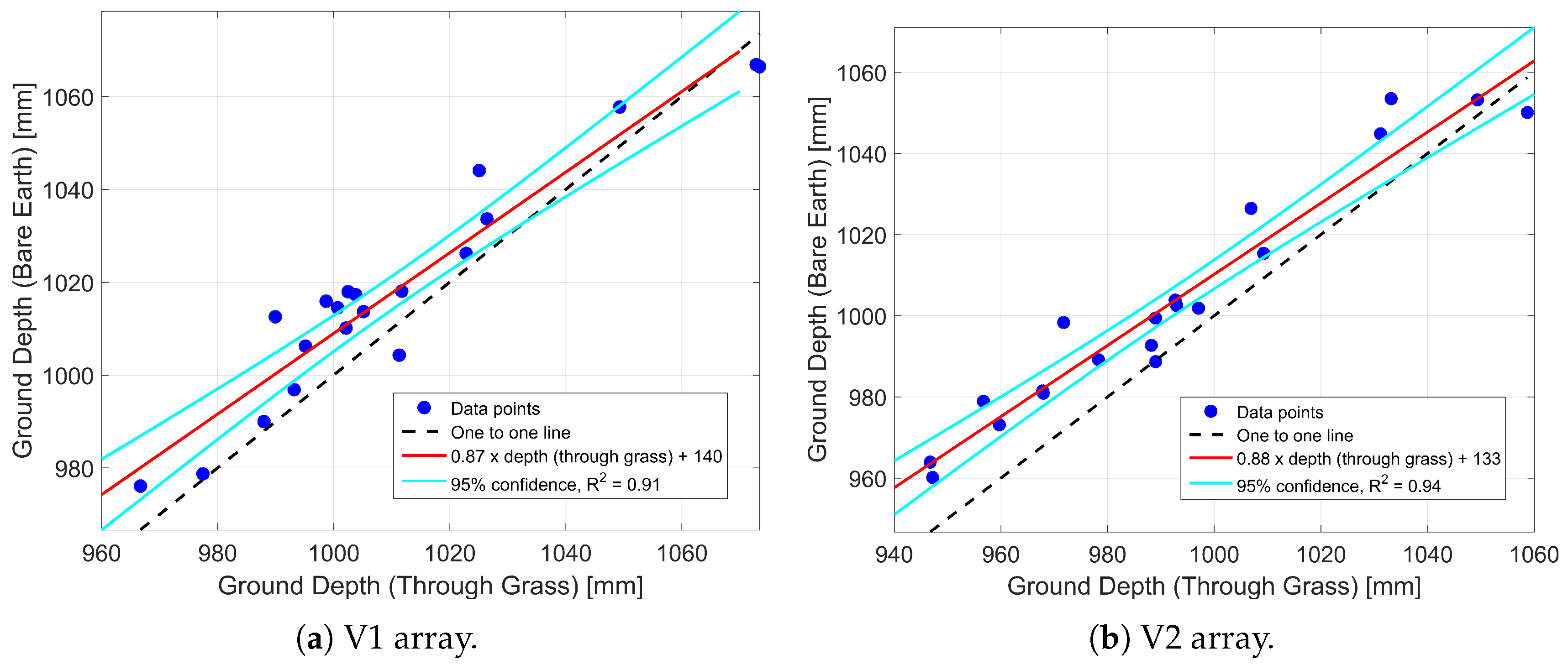
The data plotted in Figure 22 was then averaged to give a single values of , , and for each of the 20 quadrants used for biomass measurements using the cut, dry and weighing technique. Figure 23 shows a scatter plot of the averaged measured distance from the array to the ground where the measurement was made with grass or with the grass cut to bare ground. For the V2 array, these data points lie on a line of
with an value of 0.94. The V1 data points also lie on a similar line with an value of 0.91. This slight offset of the data points from the one-to-one line appears to be due to roughly 10% of the data points being incorrectly identifying as ground when they appear to be points located within the grass. This error should be able addressed using improved signal processing techniques and/or using a calibration correction such as that given in Equation (6).
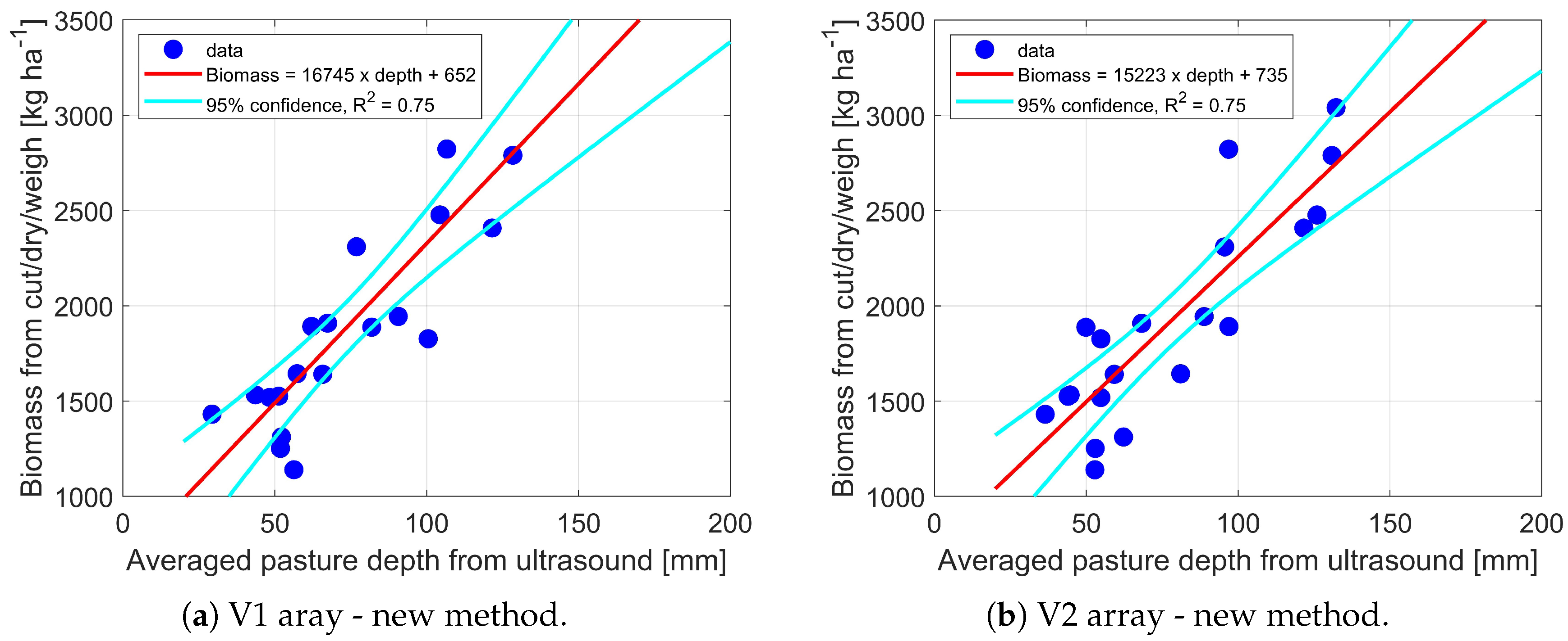
The grass height estimation was then performed. First the ground distance measurements , which were made through grass, were corrected using Equation (6). The grass height was then calculated from this using Equation (5) and averaged into twenty values, one for each 0.5 meter wide quadrant used for cut and dry biomass measurements. Figure 24 shows a scatter plot of the resulting averaged grass heights and measured biomass values for the V1 and V2 arrays. Using measurement of the actual ground location (new technique), resulted in pasture height measurements that correlated with biomass with values of 0.75 for both arrays. In contrast, when the ground height was assumed to be a set distance from the arrays, which is the traditional technique, values of 0.6 and 0.56 respectively for the V1 and V2 arrays were obtained, see Table 3. This gives roughly 25% improvement for the new technique compared with the traditional technique and gives a reduction in root mean square error (RMSE) from about 350 to 270 kg/ha.
6. Conclusions
Accurate measurement of pasture biomass is an important part of optimising the efficiency of agriculture industries that utilise pasture. Ultrasonic measurement of pasture height is one technique that can be used for estimating biomass. However, if the ultrasonic sensor is attached to a farm vehicle, tilting and bouncing of the vehicle can lead to height estimation errors. This work presents hardware that was developed to investigate if ground location could be measured directly from ultrasonic measurement of pasture. This hardware used arrays of ultrasonic transducers and microphones combined with chirp ultrasonic transmission and cross-correlation to increase the angular and depth resolution. The first version of the hardware (V1) had a fixed beamwidth of 8.7 degrees and MLS of 25 dB. However, it was not known if increased angular resolution and MLS would provide improved biomass estimation accuracy. A second version of the hardware (V2) was, therefore, developed. This was able to achieve a beamwidth of 3.3 degrees and MLS of about 33 dB.
Farm bike field trials were performed using both the V1 and V2 arrays. Example results were shown for a transect of pasture where there was variation in the slope of the ground causing the height of the ultrasonic sensors to vary over the transect. Both the V1 and V2 were able to detect the ground. Some measurements points incorrectly identified grass as ground, however, improved signal processing or calibration should be able to reduce this. We believe this paper is the first to show this ability to simultaneously measure both the pasture top and ground. The grass height was able to be measured by subtracting the ultrasonically measured distances from the sensor to the ground and to the top of the pasture. This provided an improvement of about 25% in compared for the traditional technique where the ground position was assumed to be constant. However, for flat ground, where there was no tilting of the vehicle, the benefit of measuring ground would be expected to much less.
When designing the V1 array for biomass estimation, the authors had believed that the V1 ultrasonic array had sufficient angular resolution and MLS. However, it was believed that this needed to be tested. The V2 array was, therefore, developed as a research tool to see if higher angular resolution, MLS, and ultrasonic power would improve biomass estimation performance. However, the results described above indicate that the V1 array had similar performance in terms of biomass estimation using height measurement compared to the V2 array.
7. Patents
Author Contributions
Conceptualization, S.B.; methodology, M.L. and S.B.; hardware development, M.L.; software, M.L.; validation, M.L.; formal analysis, M.L.; investigation, M.L. and S.B.; writing—original draft preparation, M.L.; writing—review and editing, M.L. and S.B.; project administration, S.B.; funding acquisition, S.B. All authors have read and agreed to the published version of the manuscript.
Funding
This work was supported by a grant from the New Zealand Ministry of Business, Innovation and Employment (MBIE) and by co-funding from Gallagher Group Ltd.
Acknowledgments
The authors would like to thank colleagues at AgResearch, particularly Warren King, for assistance with the field trials. This included cutting and drying of pasture and all driving of the farm bike. The bulk of this work was conducted at the University of Auckland where Stuart Bradley was a Professor.
Conflicts of Interest
“The authors declare no conflicts of interest”.
References
- Beukes, P.; McCarthy, S.; Wims, C.; Gregorini, P.; Romera, A. Regular estimates of herbage mass can improve profitability of pasture-based dairy systems. Anim. Prod. Sci. 2019, 59, 359–367. [Google Scholar] [CrossRef]
- Clarke, D.; Litherland, A.; Mata, G.; Burling-Claridge, R. Pasture monitoring from space. In Proceedings of the South Island Dairy Event (SIDE) Conference, Kent, UK, 26–28 June 2006; pp. 26–28. [Google Scholar]
- Ali, I.; Cawkwell, F.; Dwyer, E.; Barrett, B.; Green, S. Satellite remote sensing of grasslands: From observation to management. J. Plant Ecol. 2016, 9, 649–671. [Google Scholar] [CrossRef] [Green Version]
- Earle, D.; McGowan, A. Evaluation and calibration of an automated rising plate meter for estimating dry matter yield of pasture. Aust. J. Exp. Agric. 1979, 19, 337–343. [Google Scholar] [CrossRef]
- Angelone, A.; Toledo, J.M.; Burns, J.C. Herbage measurement in situ by electronics. 1. The multiple-probe-type capacitance meter: A brief review. Grass Forage Sci. 1980, 35, 25–33. [Google Scholar] [CrossRef]
- Murphy, W.; Silman, J.; Barreto, A.M. A comparison of quadrat, capacitance meter, HFRO sward stick, and rising plate for estimating herbage mass in a smooth-stalked, meadowgrass-dominant white clover sward. Grass Forage Sci. 1995, 50, 452–455. [Google Scholar] [CrossRef]
- López-Díaz, J.; Roca-Fernández, A.; González-Rodríguez, A. Measuring herbage mass by non-destructive methods: A review. J. Agric. Sci. Technol. 2011, 1, 303–314. [Google Scholar]
- Wachendorf, M.; Fricke, T.; Möckel, T. Remote sensing as a tool to assess botanical composition, structure, quantity and quality of temperate grasslands. Grass Forage Sci. 2018, 73, 1–14. [Google Scholar] [CrossRef]
- Chao, Z.; Liu, N.; Zhang, P.; Ying, T.; Song, K. Estimation methods developing with remote sensing information for energy crop biomass: A comparative review. Biomass Bioenergy 2019, 122, 414–425. [Google Scholar] [CrossRef]
- Sanderson, M.A.; Rotz, C.A.; Fultz, S.W.; Rayburn, E.B. Estimating forage mass with a commercial capacitance meter, rising plate meter, and pasture ruler. Agron. J. 2001, 93, 1281–1286. [Google Scholar] [CrossRef] [Green Version]
- Xue, J.; Su, B. Significant remote sensing vegetation indices: A review of developments and applications. J. Sens. 2017, 2017, 1353691. [Google Scholar] [CrossRef] [Green Version]
- Hanna, M.; Steyn-Ross, D.; Steyn-Ross, M. Estimating biomass for New Zealand pasture using optical remote sensing techniques. Geocarto Int. 1999, 14, 89–94. [Google Scholar] [CrossRef]
- Gu, Y.; Wylie, B.K.; Howard, D.M.; Phuyal, K.P.; Ji, L. NDVI saturation adjustment: A new approach for improving cropland performance estimates in the Greater Platte River Basin, USA. Ecol. Indic. 2013, 30, 1–6. [Google Scholar] [CrossRef]
- Andersson, K.; Trotter, M.; Robson, A.; Schneider, D.; Frizell, L.; Saint, A.; Lamb, D.; Blore, C. Estimating pasture biomass with active optical sensors. Adv. Anim. Biosci. 2017, 8, 754–757. [Google Scholar] [CrossRef]
- Fricke, T.; Wachendorf, M. Combining ultrasonic sward height and spectral signatures to assess the biomass of legume–grass swards. Comput. Electron. Agric. 2013, 99, 236–247. [Google Scholar] [CrossRef]
- Safari, H.; Fricke, T.; Wachendorf, M. Determination of fibre and protein content in heterogeneous pastures using field spectroscopy and ultrasonic sward height measurements. Comput. Electron. Agric. 2016, 123, 256–263. [Google Scholar] [CrossRef]
- Safari, H. Combined Use of Spectral Signatures and Ultrasonic Sward Height for the Assessment of Biomass and Quality Parameters in Heterogeneous Pastures. Ph.D. Thesis, Department of Grassland Science and Renewable Plant Resourses, University of Kassel, Witzenhausen, Germany, 2017. [Google Scholar]
- Moeckel, T.; Safari, H.; Reddersen, B.; Fricke, T.; Wachendorf, M. Fusion of ultrasonic and spectral sensor data for improving the estimation of biomass in grasslands with heterogeneous sward structure. Remote Sens. 2017, 9, 98. [Google Scholar] [CrossRef] [Green Version]
- Möckel, T.; Fricke, T.; Wachendorf, M. Multi-temporal estimation of forage biomass in heterogeneous pastures using static and mobile ultrasonic and hyperspectral measurements. In Sustainable Meat and Milk Production from Grasslands, Proceedings of the 27th General Meeting of the European Grassland Federation, Cork, Ireland, 17–21 June 2018; Teagasc, Animal & Grassland Research and Innovation Centre, Moorepark, Fermoy: Co. Cork, Ireland, 2018; pp. 813–815. [Google Scholar]
- Cao, Z.; Cheng, T.; Ma, X.; Tian, Y.; Zhu, Y.; Yao, X.; Chen, Q.; Liu, S.; Guo, Z.; Zhen, Q.; et al. A new three-band spectral index for mitigating the saturation in the estimation of leaf area index in wheat. Int. J. Remote Sens. 2017, 38, 3865–3885. [Google Scholar] [CrossRef]
- Barthram, G. Experimental Techniques: The HFRO Sward Stick; Technical Report; The Hill Farming Research Organization, Biennial Report; HFRO: Midlothian, UK, 1985. [Google Scholar]
- Cooper, S.D.; Roy, D.P.; Schaaf, C.B.; Paynter, I. Examination of the potential of terrestrial laser scanning and structure-from-motion photogrammetry for rapid nondestructive field measurement of grass biomass. Remote Sens. 2017, 9, 531. [Google Scholar] [CrossRef] [Green Version]
- Hutchings, N.; Phillips, A.; Dobson, R. An ultrasonic rangefinder for measuring the undisturbed surface height of continuously grazed grass swards. Grass Forage Sci. 1990, 45, 119–127. [Google Scholar] [CrossRef]
- Hutchings, N. Spatial heterogeneity and other sources of variance in sward height as measured by the sonic and HFRO sward sticks. Grass Forage Sci. 1991, 46, 277–282. [Google Scholar] [CrossRef]
- Hutchings, N. Factors affecting sonic sward stick measurements: The effect of different leaf characteristics and the area of sward sampled. Grass Forage Sci. 1992, 47, 153–160. [Google Scholar] [CrossRef]
- King, W.; Rennie, G.; Dalley, D.; Dynes, R.; Upsdell, M. Pasture mass estimation by the C-DAX pasture meter: Regional calibrations for New Zealand. In Proceedings of the 4th Australasian Dairy Science Symposium 2010: Meeting the Challenges for Pasture-Based Dairying, Christchurch, New Zealand, 31 August–2 September 2010; Volume 31, pp. 223–238. [Google Scholar]
- Schaefer, M.T.; Lamb, D.W. A combination of plant NDVI and LiDAR measurements improve the estimation of pasture biomass in tall fescue (Festuca arundinacea var. Fletcher). Remote Sens. 2016, 8, 109. [Google Scholar] [CrossRef] [Green Version]
- Naroaka Enterprises. Pasture Reader. Available online: http://pasturereader.com.au/ (accessed on 29 December 2019).
- Schaare, P. Improved Paster Meter. NZ Patent WO2006009472A2, 26 January 2006. [Google Scholar]
- Reusch, S. Use of ultrasonic transducers for on-line biomass estimation in winter wheat. In Precision Agriculture; Wageningen Academic Publishers: Wageningen, The Netherlands, 2009; pp. 69–175. [Google Scholar]
- Legg, M.; Bradley, S. Ultrasonic Proximal Sensing of Pasture Biomass. Remote Sens. 2019, 11, 2459. [Google Scholar] [CrossRef] [Green Version]
- Legg, M. Microphone Phased Array 3D Beamforming and Deconvolution. Ph.D. Thesis, University of Auckland, Auckland, New Zealand, 2012. [Google Scholar]
- Nakamura, K.; Gomez, R. Self-calibration of flexible microphone array for speaker localization in meeting conversations using emitters. In Proceedings of the 2018 16th International Workshop on Acoustic Signal Enhancement (IWAENC), Tokyo, Japan, 17–20 September 2018; pp. 311–315. [Google Scholar]
- Bradley, S.; Legg, M. Systems, Apparatus and Methods for Vegetation Measurement; Gallagher Group Limited: Hamilton, New Zealand, 2019; No.753949. [Google Scholar]
- Bradley, S.; Legg, M. Vegetation Measurement Apparatus, Systems, and Methods; Gallagher Group Limited: Melbourne, Australia, 2019; No.2019201425. [Google Scholar]
Figure 1.
Diagram illustrating the effect of different angular and depth resolutions on the ability to distinguish ultrasonic echoes from a particular depth in the pasture.
Figure 1.
Diagram illustrating the effect of different angular and depth resolutions on the ability to distinguish ultrasonic echoes from a particular depth in the pasture.

Figure 2.
Example of a simulated far-field beam pattern of an ultrasonic array composed of a single main lobe and sidelobes. Indicated on the plot are the key array design parameter beamwidth and maximum side lobe level (MSL) values.
Figure 2.
Example of a simulated far-field beam pattern of an ultrasonic array composed of a single main lobe and sidelobes. Indicated on the plot are the key array design parameter beamwidth and maximum side lobe level (MSL) values.

Figure 3.
Measured farm quad bike noise signal and spectra obtained using a wide frequency bandwidth microphone (Panasonic WM61A with custom built preamplifier).
Figure 3.
Measured farm quad bike noise signal and spectra obtained using a wide frequency bandwidth microphone (Panasonic WM61A with custom built preamplifier).

Figure 4.
Murata MA40H1S-R surface mount transducer.

Figure 5.
Measured transmit signals for a range of transducers obtained using a microphone for five-cycle Hamming windowed sine wave transmit signal. The top transducer in each plot is the Murata MA40H1S-R transducer.
Figure 5.
Measured transmit signals for a range of transducers obtained using a microphone for five-cycle Hamming windowed sine wave transmit signal. The top transducer in each plot is the Murata MA40H1S-R transducer.

Figure 6.
Microphone recordings showing the variation in ringing with transmit frequency of the Murata MA40H1S-R transducer output signal for a five-cycle Hamming windowed sine wave. Overlaid in red is the signal applied to the transducer.
Figure 6.
Microphone recordings showing the variation in ringing with transmit frequency of the Murata MA40H1S-R transducer output signal for a five-cycle Hamming windowed sine wave. Overlaid in red is the signal applied to the transducer.

Figure 7.
Measured normalised frequency and angular gain of the Murata MA40H1S-R transducer.

Figure 8.
(a) Photo of “version 1” ultrasonic array printed circuit board. (b) Simplified diagram of how array elements are connected to steer the array in a single direction.
Figure 8.
(a) Photo of “version 1” ultrasonic array printed circuit board. (b) Simplified diagram of how array elements are connected to steer the array in a single direction.

Figure 9.
Simulated far-field beam patterns for V1 array at 30 kHz for transmission (a) and reception (b).
Figure 9.
Simulated far-field beam patterns for V1 array at 30 kHz for transmission (a) and reception (b).

Figure 10.
Photo of the version 2 array transmit/receive PCB.

Figure 11.
V2 amplifier printed circuit board (PCB) board.

Figure 12.
Simplified diagram of the V2 hardware. Diagram (a) shows how relays are used to control which of the 10 transducer rings are used for transmission. Diagram (b) shows how an individual ADC is used for each microphone ring.
Figure 12.
Simplified diagram of the V2 hardware. Diagram (a) shows how relays are used to control which of the 10 transducer rings are used for transmission. Diagram (b) shows how an individual ADC is used for each microphone ring.

Figure 13.
Simulated far-field transmission beam patterns for the V2 hardware showing how the beamwidth and MLS can be adjusted by adjusting which transducer rings are used for transmission.
Figure 13.
Simulated far-field transmission beam patterns for the V2 hardware showing how the beamwidth and MLS can be adjusted by adjusting which transducer rings are used for transmission.

Figure 14.
Simulated far-field reception beam patterns for the V2 hardware showing how the beamwidth and MLS can be adjusted by adjusting which microphone rings are used for reception.
Figure 14.
Simulated far-field reception beam patterns for the V2 hardware showing how the beamwidth and MLS can be adjusted by adjusting which microphone rings are used for reception.

Figure 15.
Plots of simulated MSL and beamwidth for V2 arrays as a function of the number of rings (from the center) used for transmission and reception. (Simulation does not include transducer directivity).
Figure 15.
Plots of simulated MSL and beamwidth for V2 arrays as a function of the number of rings (from the center) used for transmission and reception. (Simulation does not include transducer directivity).

Figure 16.
Photo (a) shows the V1 and V2 arrays mounting for farm bike trials. Photo (b) shows the experimental setup used for beam pattern measurements.
Figure 16.
Photo (a) shows the V1 and V2 arrays mounting for farm bike trials. Photo (b) shows the experimental setup used for beam pattern measurements.

Figure 17.
Plot (a) shows the measured transmit/receive 3D beam pattern for the V2 array for 30 kHz sine wave transmit signal for all microphones and transmitter rings used. Plot (b) shows a comparison of the corresponding 1D the beam patterns for the V2 and V1 arrays.
Figure 17.
Plot (a) shows the measured transmit/receive 3D beam pattern for the V2 array for 30 kHz sine wave transmit signal for all microphones and transmitter rings used. Plot (b) shows a comparison of the corresponding 1D the beam patterns for the V2 and V1 arrays.

Figure 18.
Example of measured 1D beam patterns for the V2 array showing how the beamwidth and signal to noise ratio changes as the speaker and microphone rings used for transmission and reception are varied.
Figure 18.
Example of measured 1D beam patterns for the V2 array showing how the beamwidth and signal to noise ratio changes as the speaker and microphone rings used for transmission and reception are varied.

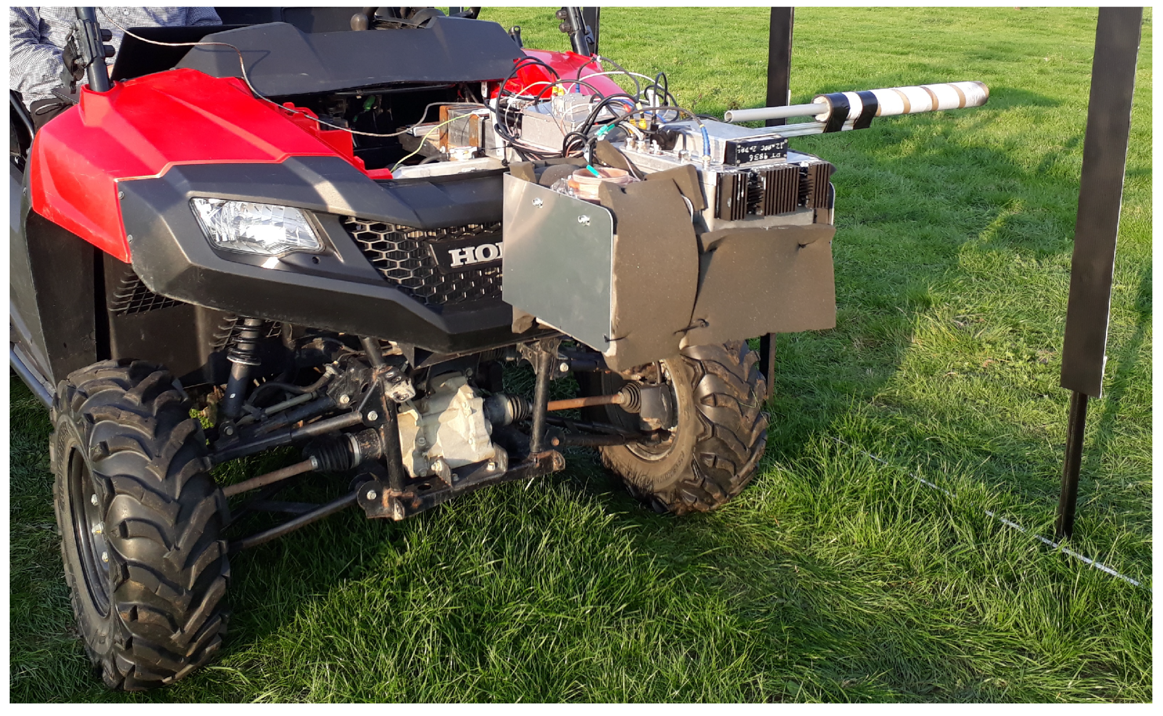
Figure 19.
V1 and V2 arrays attached to a farm bike for field trials.

Figure 20.
Photo (a) shows “Transect 2” which was used for bike field trials. The black cards on posts were used for localisation of ultrasonic measurements using the IR sensor. Photo (b) shows the same transect with the grass cut to the ground for cut, dry and weigh biomass measurements.
Figure 20.
Photo (a) shows “Transect 2” which was used for bike field trials. The black cards on posts were used for localisation of ultrasonic measurements using the IR sensor. Photo (b) shows the same transect with the grass cut to the ground for cut, dry and weigh biomass measurements.

Figure 21.
Example ultrasonic signal made while the bike was driving over pasture. The part of the signal assumed to corresponding to ground and top of the grass are indicated.
Figure 21.
Example ultrasonic signal made while the bike was driving over pasture. The part of the signal assumed to corresponding to ground and top of the grass are indicated.

Figure 22.
Plot showing individual (not averaged) measurements of the distance from the array to the grass top and to the ground for the V1 and V2 arrays. Roughly 10% of the ground measurement made through grass (black dots) appear to be located above the scatter of measurements made for bare ground (blue dots).

Figure 23.
Comparison of averaged measured distances of the V1 and V2 arrays to the ground when measured through grass or to bare earth. These measurements were averaged to give a single distance measurement twenty 0.5 × 0.5 m wide quadrants used for biomass cut and weight measurements.
Figure 23.
Comparison of averaged measured distances of the V1 and V2 arrays to the ground when measured through grass or to bare earth. These measurements were averaged to give a single distance measurement twenty 0.5 × 0.5 m wide quadrants used for biomass cut and weight measurements.

Figure 24.
Scatter plot showing the fit between biomass and averaged pasture height measurement using ground measurements.
Figure 24.
Scatter plot showing the fit between biomass and averaged pasture height measurement using ground measurements.


Table 1.
Details of versions 1 and 2 array boards. TX and RX, respectively, refer to the transmission and receiver sub-arrays.
Table 1.
Details of versions 1 and 2 array boards. TX and RX, respectively, refer to the transmission and receiver sub-arrays.
| V1 | V2 | |||
|---|---|---|---|---|
| PBC Diameter (mm) | 80 | 190 | ||
| Transmit/Receive Array | TX | RX | TX | RX |
| Array Diameter (mm) | 61 | 61 | 150 | 150 |
| Total No. of Elements | 29 | 28 | 160 | 204 |
| No. of Spiral Arms | 7 | 7 | 17 | 17 |
| No. of Rings (or No. Elements Per Arm) | 4 | 4 | 10 | 12 |
Table 2.
Measured beam pattern parameters for V1 and V2 arrays for 0.5 ms duration 20–35 kHz chirp excitation signal. Different configurations of transmit and receive rings were used for the V2 array. Note that the beamwidth was calculated from the horizontal position at a range of 805 mm.
Table 2.
Measured beam pattern parameters for V1 and V2 arrays for 0.5 ms duration 20–35 kHz chirp excitation signal. Different configurations of transmit and receive rings were used for the V2 array. Note that the beamwidth was calculated from the horizontal position at a range of 805 mm.
| Version | Transducer Rings | Receiver Rings | Beamwidth | MSL |
|---|---|---|---|---|
| V1 | – | – | 122 mm (8.7°) | 25 dB |
| V2 | 1 | 1 | 148 mm (10.5°) | 10 dB |
| V2 | All | 1 | 66 mm (4.7°) | 15 dB |
| V2 | 1 | All | 63 mm (4.5°) | 27 dB |
| V2 | All | All | 46 mm (3.3°) | 33 dB |
Table 3.
Measured and root mean square error (RMSE) values obtained for the fit between biomass and the averaged ultrasonic grass height measurements for the traditional method, where the ground location was assumed to be a fixed value and the new technique where the ground position is measured.
Table 3.
Measured and root mean square error (RMSE) values obtained for the fit between biomass and the averaged ultrasonic grass height measurements for the traditional method, where the ground location was assumed to be a fixed value and the new technique where the ground position is measured.
| Hardware Version | Traditional Method | New Method |
|---|---|---|
| V1 | ||
| RMSE = 342 kg/ha | RMSE = 272 kg/ha | |
| V2 | ||
| RMSE = 359 kg/ha | RMSE = 267 kg/ha |
© 2019 by the authors. Licensee MDPI, Basel, Switzerland. This article is an open access article distributed under the terms and conditions of the Creative Commons Attribution (CC BY) license (http://creativecommons.org/licenses/by/4.0/).
Share and Cite
MDPI and ACS Style
Legg, M.; Bradley, S. Ultrasonic Arrays for Remote Sensing of Pasture Biomass. Remote Sens. 2020, 12, 111. https://0-doi-org.brum.beds.ac.uk/10.3390/rs12010111
AMA Style
Legg M, Bradley S. Ultrasonic Arrays for Remote Sensing of Pasture Biomass. Remote Sensing. 2020; 12(1):111. https://0-doi-org.brum.beds.ac.uk/10.3390/rs12010111
Chicago/Turabian StyleLegg, Mathew, and Stuart Bradley. 2020. "Ultrasonic Arrays for Remote Sensing of Pasture Biomass" Remote Sensing 12, no. 1: 111. https://0-doi-org.brum.beds.ac.uk/10.3390/rs12010111
Note that from the first issue of 2016, this journal uses article numbers instead of page numbers. See further details here.