A Review of RFI Mitigation Techniques in Microwave Radiometry


1
Interdisciplinary Centre for Security, Reliability and Trust (SnT), University of Luxembourg, 29 Avenue John F. Kennedy, L-1855 Luxembourg, Luxembourg
2
Unidad María de Maeztu CommSensLab-UPC, Dept. of Signal Theory and Communications, Universitat Politècnica de Catalunya (UPC)—BarcelonaTech, C/Jordi Girona 1-3, 08034 Barcelona, Spain
*
Author to whom correspondence should be addressed.
Remote Sens. 2019, 11(24), 3042; https://0-doi-org.brum.beds.ac.uk/10.3390/rs11243042
Submission received: 29 October 2019
/
Revised: 3 December 2019
/
Accepted: 13 December 2019
/
Published: 17 December 2019
(This article belongs to the Special Issue Radio Frequency Interference (RFI) in Microwave Remote Sensing)
Abstract
:Radio frequency interference (RFI) is a well-known problem in microwave radiometry (MWR). Any undesired signal overlapping the MWR protected frequency bands introduces a bias in the measurements, which can corrupt the retrieved geophysical parameters. This paper presents a literature review of RFI detection and mitigation techniques for microwave radiometry from space. The reviewed techniques are divided between real aperture and aperture synthesis. A discussion and assessment of the application of RFI mitigation techniques is presented for each type of radiometer.
1. Introduction
Radio frequency interference (RFI) signals are unwanted electromagnetic emissions that degrade the performance of a receiver. Currently, the concerns about RFI are increasing because of the high number of detected occurrences, and this problem is expanding because of the extensive use and abuse of wireless technologies around the world. RFI signals are emitted illegally in bands reserved for passive observations (in-band RFI), or legally in adjacent bands, but a fraction of their power leaks into the radiometer bandwidth (near-band effect), or from harmonics of emissions at a much lower frequency band or from intermodulation products (out-of-band effect). The origin of RFI signals can be from different sources. RFI can be intentional or unintentional, and it can be generated externally or by the same device (self-interference), although self-interference should be minimized by proper design. RFI signals can even be intentional emissions (jamming) designed to override a particular frequency band. According to [1], the allocated bands provide a statutory protection, with no guarantees against interference occurrences from accidental out-of-band emissions to intentional jamming.
Therefore, RFI has become a dangerous threat for passive remote sensing and, in particular, for microwave radiometry (MWR), which is used to measure a large number of geophysical parameters, such as ice and snow cover, soil moisture, sea surface salinity, wind speed over the sea, sea ice concentration, rain rate, atmospheric temperature and water vapor profiles, cloud liquid water content, etc. [2]. To achieve these goals, microwave radiometers must have high sensitivity requirements, in the order of 1 Kelvin or less (see Table 1).
Although MWR operates in “protected” frequency bands, because of their high sensitivity requirements, microwave radiometers are easily affected by RFI signals. This effect is even more noticeable in secondary band allocations. As stated in [4], passive Earth observation is likely going to be affected more and more by active commercial services. A priori, any of the allocated frequency bands for Earth observation can be affected by RFI, however lower bands are more likely to be affected because of the higher density of spectrum use. The most prominent example of a contaminated band is the L-band (1.4 GHz), but RFI cases have also been reported at C-band (6.8 GHz) [4], X-band (10.7 GHz) [5], and K-band (18.7 GHz) [6].
The presence of RFI signal increases the total power in the band, which translates into a positive bias in the measured brightness temperature (BT). The final outcome of RFI contamination is that an error is introduced in the geophysical variable being observed. For example, soil moisture maps contaminated by RFI show apparent dryer soils than they actually are [7], while sea surface salinity maps affected by (small) RFI show a lower salinity. Furthermore, typical RFI power levels are much higher than the radiometric noise power, and MWR measurements are totally corrupted. According to [8], the rationale is that natural Earth emissions are not expected to produce BT measurements that exceed 330 K, but many RFI emissions are stronger than 500 K. Several publications from current missions, such as SMOS [9] and SMAP [10], show antenna temperatures larger than 1000 K from high contaminated areas such as Europe, Middle East, Eastern China, and Japan. However, weak RFI is even more disturbing, as it is more difficult to detect, and often to eliminate, and pass undetected.
RFI signals disrupt all types of microwave radiometers. The most common distinction between types of radiometers is their antenna configuration. Real aperture radiometers use a single antenna, whereas synthetic aperture radiometers have an interferometric array of antennas. The different antenna configuration distinguishes between the RFI mitigation techniques for real aperture, and afterwards, extends them to the more complex case of synthetic aperture.
This paper is structured as follows: Section 2 provides a review of RFI detection and mitigation techniques in real aperture radiometers. Section 3 presents a discussion on RFI detection and mitigation for real aperture radiometers. Section 4 provides a review of RFI detection and mitigation techniques in synthetic aperture radiometers. Section 5 presents a discussion on RFI detection and mitigation for synthetic aperture radiometers. Finally, Section 6 states the conclusions of this manuscript.
2. Review of RFI Detection and Mitigation Techniques in Real Aperture Radiometers
The literature on RFI detection and mitigation (D/M) in passive microwaves (radiometry and GNSS-R) has consolidated a number of techniques in the past years. Any RFI mitigation technique requires early detection of the presence of an RFI signal. The literature of RFI D/M covers several fields such as microwave radiometry, radio astronomy, and navigation, however D/M in active microwave sensors or communications is out of the scope of this review.
Existing D/M techniques can, first, be classified as follows:
- Parametric techniques designed to mitigate a particular type of RFI signal (e.g., a continuous wave or CW signal);
- Nonparametric techniques agnostic of the particular type of RFI signal.
These techniques can also be classified according to their domain of operation (see Figure 1) as follows:
- Time domain, such as pulse blanking or time gating;
- Frequency domain, such as frequency blanking or adaptive notch filtering;
- Statistical domain, such as normality tests and goodness-of-fit tests;
- Polarimetry domain, such as Stokes parameters test or antennas with high cross-polar isolation;
- Space domain, such as beamforming or null-steering antennas.
According to [11], the performance of each technique is highly dependent on the RFI scenario, for example, power, number of simultaneous RFI signals, direction of arrival (DOA), time repeatability, bandwidth, polarization, etc. Unfortunately, since there are many different types of RFI signals, and they can coexist simultaneously, there is no optimum technique for all signals and a combination of techniques must be implemented. Therefore, this explains the development of RFI D/M algorithms that combine several domains such as:
- Time-statistical, such as time kurtosis or amplitude domain processing (ADP) [12];
- Time-frequency, such as spectrogram blanking [13];
- Frequency-statistical, such as spectral kurtosis [14];
- Time-scale, such as wavelets [15];
- Time-frequency-scale, such as multiresolution Fourier transform [16] and wavelet packet decomposition (WPD);
In most cases, the problem of RFI involves the detection of stochastic signals with, a priori, unknown parameters. Therefore, the RFI detection criterion should be based on the Neyman–Pearson hypothesis to test the discrimination between RFI-contaminated samples and RFI-clean samples defined by a threshold value α. A tradeoff between the probability to detect RFIs (probability of detection, PD) and the probability to eliminate RFI-clean data falsely (probability of false alarm, PFA) must be accomplished. The PFA depends on the probability density function (PDF) of the received signal in the absence of RFI. Thus, it is always determined since the RFI-free signal has a Gaussian (i.e., normal) distribution in remote sensing (microwave radiometry) and almost Gaussian (SNR << 0 dB) in GNSS applications. Note that Gaussian distribution applies to either samples of real signal radiometers or each of the components of an I/Q front-end. Hence, if s[n] = s is the digital sampled signal at the receiver, s follows a Gaussian distribution, and f(s) ∼ N (0, σ2) is the PDF of s, then,
where
is the so-called Q-function defined as the tail probability of the standard normal distribution [21]. However, the undetermined parameters of the RFIs lead to a lack of knowledge of the PD.
There are several methods used to combat RFIs, but the choice of technique depends on several factors such as cost, space constraints, power consumption, and the environment where they are used [22]. A short summary of most well-known methods is presented in subsequent sections.
2.1. Time Domain Techniques
The time domain RFI mitigation algorithm is the simplest technique, because it only requires the received signal s[n] to be sampled, and its power compared to a determined threshold α, which is directly related to the power of the RFI-free signal [23]. Hence, the most straightforward case of this technique would be to assign the output signal y[n] = f(s[n], α) as
with α = σfree*f(PFA) being σfree the standard deviation of the RFI-free signal.
This type of RFI excision is most effective with strong and short (spikes) RFI bursts. Weak and long-lasting RFI signals are more problematic because temporal domain threshold methods do not work [23]. In addition, because the detected power is a smoothed (averaged) version of the instantaneous one, if the duration of the RFI peaks is shorter than the integration time, they can pass undetected [24].
2.2. Frequency Domain Techniques
RFI signals that belong to the group of CW narrowband signals, with either fixed or variable frequency, are very likely to be received in urban environments [25]. Two approaches are distinguished inside the techniques devoted to detecting these kinds of signals.
2.2.1. Non-parametric Methods
This first group of techniques includes detection algorithms based on non-parametric spectral estimation of the incoming signal, obtained by applying signal processing techniques such as the periodogram [26,27] or simply the discrete Fourier transform (DFT). In non-parametric methods, the RFI excision is typically performed by comparing the spectrum of the received signal with a theoretical threshold α usually determined according to a statistical model representing the received signal. In this context, these mitigation techniques have the same effect as notch filtering removing the interference frequency components.
Nevertheless, this approach cannot be considered the best option for non-stationary interference removal. A real interference environment is characterized by the appearance of pulsed signals, dynamics of interference, spectral characteristics changing quickly in time, and nonstationary behavior. Therefore, the use of spectral techniques that represent the signal only in spectral domain becomes an incomplete representation unable to follow the nonstationary nature of RFIs.
2.2.2. Parametric Methods
Model-based or parametric spectral estimators were proposed as a mitigation technique for jammers generating chirp signals, typical of most recently available commercial jammers [25]. The broadband nature of the chirp signal creates an average impact on the receiver similar to an increase in the thermal noise floor. However, the chirp signal is instantaneously narrowband, and this feature is exploited by a time-dependent notch filter [28]. For instance, in [29], an adaptive notch filter with transfer function
where k is the pole contraction factor and z0[n] is the filter’s zero. This approach has been simulated with successful results mitigating chirp RFIs in GNSS applications.
These adaptive notch filters are very effective for narrowband jammers and can be used in applications that require low power and small size. Their main disadvantage is that they cannot be used when the jammer does not have a predictable signal structure [18,25].
Frequently, these techniques can only track a CW signal. In [30], a two-pole notch filter coupled with a detection unit has been used as a basic element for the design of a multipole filter capable of efficiently removing more than one CW interference. The derived results provide useful information for the design of mitigation and detection units based on the adaptive notch filters that result in a computationally effective solution for CW interference mitigation.
2.3. Time-Frequency Space Techniques
Time-frequency space techniques are most widely used to detect and mitigate real nonstationary RFI signals. This approach takes into account the coexistence of the RFI signals in both time and frequency domains, thus, able to detect CW and pulsed signals simultaneously. Nevertheless, resolution in temporal domain, σt, and in frequency domain, σw, are related and constrained by the so-called Gabor limit [31] (the equivalent of the Heisenberg uncertainty principle in the context of signal processing) that satisfies
Furthermore, time-frequency space filtering tries to represent the received signal in such a way that the jammer and the signal are more easily distinguished, particularly for narrowband RFI signals due to the nature of the Fourier kernel in this transform [32]. Therefore, since the thermal noise is a low power and wideband signal, the high-power jammer signals can usually be distinguished easily in the time-frequency (TF) space [13].
Several TF distributions such as the spectrogram and Wigner–Ville distribution can be used to represent the signal in time-frequency space. The only remaining problem is the correct selection of the appropriate threshold to excise the jammer from the received signal to obtain the useful signal by transforming it back to the time domain. In [33], the calculation of the threshold according to the a priori probability of false alarm is explained. The main disadvantage of these methods is that the RFI signal or jammer can be effectively separated only if its power is sufficiently stronger than the radiometric signal itself.
2.3.1. Time-Frequency Implementations
The most common TF implementation forms are the following:
Short-time Fourier transform (STFT) STFT-based techniques are used for narrowband RFI and they can be implemented in situations that require low power and small form factor devices. The STFT [26] essentially consists of a moving window w[n] to weight a segment of the signal s[n], and then takes the DFT of the windowed region. So that,
and the so-called spectrogram is defined as
This approach can adapt rapidly to changing environments. The signal is filtered in the time-frequency space in order to remove the RFI components before being transformed back to the time domain. Furthermore, the proper choice of the window function determines the spectral leakage in the frequency-domain and the length of the temporal response [26].
Filter bank This technique has all the advantages of STFT and it can be implemented in situations that require low power consumption, small size, and poor frequency resolution. Conversely, if a high frequency resolution is desired, filter bank becomes inefficient due to the high number of filters needed, whereas STFT tends to be optimum. In [34], the filter bank technique is used in a microwave radiometer due to its good properties.
Wigner–Ville distribution (WVD) The WVD is a TF distribution that belongs to the group of quadratic time-frequency representations and it is based on the calculation of the Fourier transform (FT) of the so-called ambiguity function (AF). The AF is a general representation of the signal autocorrelation function for nonstationary stochastic processes. So that, if
the WVD yields to
The WVD does not suffer from leakage effects as the STFT does, thus, it provides the best spectral resolution. However, if the analyzed signals contain several RFI signals, the WVD suffers from the so-called cross terms. These cross terms can be partly suppressed by smoothing the WVD with low-pass two-dimensional (2D) windows [35]. Furthermore, mitigated signals cannot be retrieved directly from WVD since it is a quadratic time-frequency representation, and its implementation is not as efficient as the STFT in terms of hardware resources.
2.3.2. Time-Frequency Resolution
The amount of spectral leakage in the DFT output is determined by the selected window coefficients. To illustrate this, let us consider the non-windowed processing, which is equivalent to using a rectangular window. The Fourier transform of the rectangular window is a sinc function with the first sidelobe 13 dB below the main lobe, and subsequent sidelobes falling off at 6 dB/octave. Therefore, the signal’s energy spreads significantly across the spectrum and selecting a window with lower sidelobes reduces the amount of spectral leakage, at the expense of a wider main lobe (i.e., poorer frequency resolution).
According to [36], the Gaussian window is the most concentrated one in time and frequency, simultaneously, and it achieves the uncertainty lower bound. However, it has a wider main lobe, and thus offers poorer spectral resolution of nearby kernels. On the contrary, the rectangular window provides the best spectral resolution of nearby kernels (since it has the narrowest main lobe), but it is unusable in restricted bandwidth applications because the high sidelobe levels and spectral leakage. Several other windows such as the triangle window, trapezoidal window, Hann window, and Hamming window offer a tradeoff between the spectral resolution and spectral leakage, but they do not have a constant time amplitude like the rectangular window. Eventually, in [37], a new family of windows with minimum time-bandwidth product σt·σw for a given σt were derived from the Gaussian window, surpassing in performance all popular windows including the truncated Gaussian window.
2.4. Other Transform-Based Techniques
As mentioned above, the number of potential combinations of different domains is large. This subsection presents two of the most prominent examples beyond combinations using the frequency domain. To perform RFI excision many subspace processing techniques can be applied. In these cases, the estimation of the jammer signal can be obtained if the jammer signal is orthogonal to the useful signal in such subspace [22]. Two of the most relevant of them are the wavelet and the Karhunen–Loève transforms.
2.4.1. Wavelet Transform
Wavelet transform (WT) is a generalization of the linear transforms that have a kernel that is finite time, such as the STFT.
The set of orthogonal basis functions employed for the computation of the STFT can be understood as a set of bandpass filters with equal frequency bandwidths, representing a set of time windows with equal duration. However, it is clear that high frequency phenomena require short windows in the time domain to be observed, and low frequency phenomena require long windows. In other words, narrow windows help to effectively localize the rapidly varying portion of the signals, at the expense of a loss of information in the steady part of the signal, which is better characterized by longer windows.
In order to overcome the above issues, a set of functions is needed to better match the frequency components of the signal. Thus, a transformation is needed based on windows which are functions of both time and frequency in such a way that their bandwidths become narrower as the frequency decreases. These requirements are accomplished by using basis functions to perform the WT. Eventually, the frequency term is mostly replaced by a scaling operation to have a clear boundary to the Fourier transformation [38]. The concept of non-constant division of a signal in frequency domain is summarized in Figure 2.
2.4.2. Karhunen–Loève Transform
The Karhunen–Loève transform (KLT) is the unique subspace transform whose kernel is calculated from its own input data [41]. This approach is also known as principal component analysis (PCA) or eigenvalue decomposition (EVD). In [42,43], the performance of the KLT to detect weak RF signals is analyzed, and how this technique can be extended to the GNSS scenario offering several advantages with respect to the other approaches.
As compared to the DFT, the main advantages of the KLT are the following:
- The KLT performs equally well for narrowband and wideband signals, while the DFT is optimized for narrowband signals only;
- When comparing the base functions of the KLT and the DFT, one realizes that the KLT is a more flexible transform, as its basis functions can be of any form, resulting in a better signal decomposition. On the contrary, the DFT kernel are limited to sinusoidal functions;
- As compared to the DFT, the KLT combines deterministic and stochastic signal analyses, which is a very powerful and unique attribute. The KLT ranks the basis functions with respect to their probable power contribution, thus, efficiently distinguishing the signal from the noise. This means that the KLT can filter the signal keeping only the most interesting, non-stochastic part and omitting the rest (i.e., background noise);
- Finally, the KLT is able to detect much weaker signals than the DFT [41]. Although it still has to be confirmed in practical applications, it could have an enormous future potential.
The underlying idea of this method is the decomposition of the signal in a vector space using eigenfunctions, which can have, in principle, any shape, and therefore can better adapt to the processed signal. A noisy signal is characterized by a KLT with only small eigenvalues, therefore, the presence of larger eigenvalues indicates the presence of deterministic signals buried in the noise. Indeed, the most significant benefit of the KLT transform is its capability of successful detection. This technique increases the detection performance not only of CW, but also to narrowband, wideband, and chirp RFIs, which are usually arduous to handle.
Nevertheless, the most significant drawback of the KLT technique is its complexity and the computational burden required to extract a very large number of eigenvalues and eigenfunctions. A possible improvement is achieved by the bordered autocorrelation method KLT (BAM-KLT), which in principle reduces the complexity but limits the detection performance [42].
An example of KLT application is found in [43], where a rank tracking device based on the evaluation of the covariance matrix eigenvalues of the observed data record evaluate the number of detected RFI signals.
2.5. Statistical Domain Techniques
Since the RFI and the desired signal are assumed to be independent stochastic processes, they can have different statistical properties that can be used to separate them. The statistical domain techniques, also coined amplitude domain processing (ADP) in [44], are tools able to distinguish between samples that belong to different statistical distributions. Normality tests are the most widely used and they try to find out if a set of samples belongs (or how similar it is) to the normal (Gaussian) statistical distribution. The rationale behind the use of normality tests to detect RFI in microwave radiometry, as well as in navigation applications, is that the useful signals follow a zero mean Gaussian distribution, whereas, in general, man-made RFI are non-Gaussian.
In [45], ten different normality tests were analyzed in terms of their RFI detection capability. These tests were first validated in terms of sequence length and number of quantization bits in the absence of interference. It was found that kurtosis is the best RFI detection algorithm for almost all types of RFI, although it exhibits a blind spot for sinusoidal and chirp interfering signals of 50% duty cycle [46]. Moreover, the above-mentioned study suggests that the Anderson–Darling (A-D) test could be a complementary normality test that covers the kurtosis blind spot, and it has a very good performance for all the studied sample sizes. Other known normality tests are the Shapiro–Wilk and the Jarque–Bera, but they do not perform as well as the kurtosis test [45]. Examples of the kurtosis test in combination with time-frequency techniques are found in [34].
Nevertheless, the combination of normality test techniques with other detection and mitigation techniques can be troublesome. In addition, the Gabor limit is a well-known low boundary for the product of time and frequency resolution, statistical, and other domains are also linked in some way. This boundary is determined by the central limit theorem (CLT) [47]. For example, in [47], a normality test is applied after a DFT and a FIR filter, respectively, without taking into account that these transformations introduce a normalization effect in the original samples due to the CLT. In some way, the product between the resolution in the statistical and time domains has a lower boundary as in the TF case.
Moreover, another approach for the normality tests is shown in [44] where ADP techniques modify the amplitude of each digital sample in such a way that non-Gaussian interferences are suppressed, resulting in an improvement in SNR. The calculation of the optimal non-linear mapping is based on the statistical decision theory and acts to de-emphasize those samples in which signal detection is unlikely. To calculate the nonlinear mapping, the signal’s amplitude probability density function has to be estimated. One of the main advantages of the amplitude domain processing is that it can reject very fast sweeping interferences, as it does not need to track the interference frequency.
Statistical techniques can also be applied in the frequency-domain. For example, the spectral kurtosis is a statistical quantity that is low when data is stationary and Gaussian, and high at transients, therefore, it can be used to detect and locate nonstationary or non-Gaussian behavior. This technique has been proposed to detect or mitigate RFI in ESA CHIME mission [48].
2.6. Spatial Domain Techniques
Adaptive antennas use spatial domain filtering techniques to cancel the RFI signal. As in adaptive filtering, these techniques are based on the optimization cost function and can be adapted for narrowband and wideband RFI signals. However, they are able to handle a large number of RFI signals in different locations simultaneously, as the maximum number of nulls in the antenna pattern is determined by the number of antenna elements [49]. The two basic approaches to spatial filtering are null steering and beamforming [22] described as follows:
- Null steering uses the simple concept that remote sensing signals are much below the thermal noise level, and hence any signal that has a power above the thermal noise has to be an interfering signal. The antennas in the array are weighted so that any particular signal can be canceled. Null steering constantly computes the weights in order to minimize the received energy level. In effect, this technique attempts to steer the antenna away from the RFI source. This method has the disadvantage of potentially reducing the signal level.
- Beamforming tries to adjust the antenna in order to maximize the SNR. In effect, the antenna beam is steered in the direction of the desired signal. If the direction to the desired source is known, beamforming can effectively maximize the SNR. It is, however, possible to end up in situations where the RFI source is in the same direction as the signal source.
Spatial filters reject the interference in angle, rather than time or frequency, and they can achieve large mitigation margins against most interference waveforms, including broadband noise. Spatial filters require multi-element antenna arrays, which are significantly larger and heavier than single element antennas. This leads to a system that can cancel up to the number of elements in the antenna minus one [22]. Combining spatial and frequency filtering allows nulls to be steered in both angle and frequency.
For example, in [50], a number of requirements for GNSS antennas are derived in order to ensure that critical infrastructure timing receivers have access to a sufficient number of satellites to derive resilient time and frequency, while placing a null in the gain pattern in the direction of the horizon and around all azimuth angles to suppress ground-based interference.
2.7. Polarization Domain Techniques
Polarization domain techniques use the unique physical property of the electromagnetic fields, the polarization, to distinguish between RFI or useful signals. In conventional radiometry, the monitoring of the third and fourth elements of the Stokes parameters of the data coming from a dual-linear polarization antenna can be a very simple solution for the detection of RFI signals. As compared to spatial filters, the main advantage of this technique is that it only requires a single antenna element (with dual polarization), and therefore it is significantly lighter and cheaper. However, as in the statistical domain case, polarization techniques can only be used to eliminate an entire set of samples.
3. Discussion on Real Aperture Radiometers RFI Detection and Mitigation
3.1. Assessment of RFI Mitigation Techniques
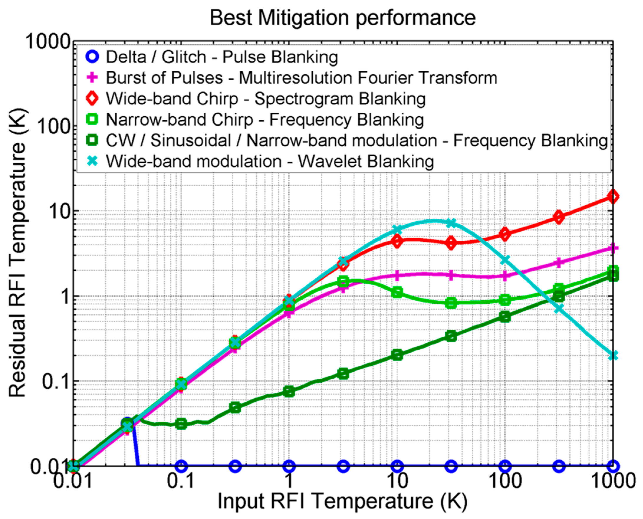
In [33], the optimum D/M technique for each type of RFI is analyzed and quantified in terms of the residual RFI temperature in Kelvin, with respect to the input RFI equivalent noise temperature in Kelvin. Results are summarized in Figure 3.
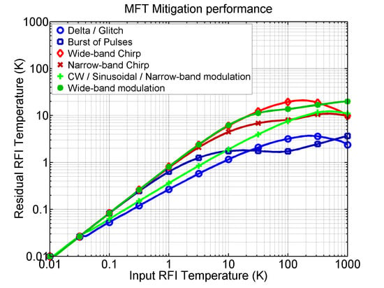
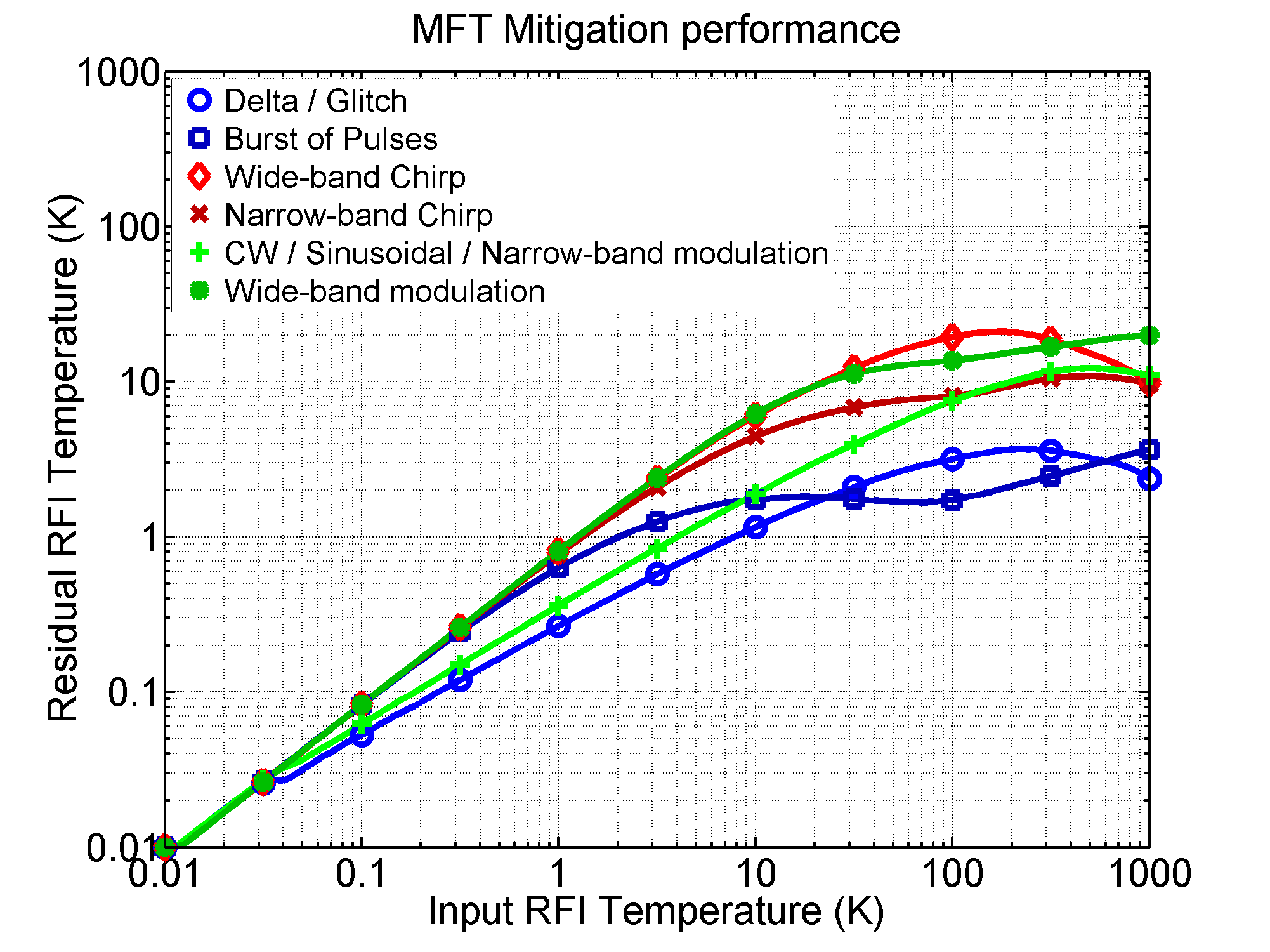
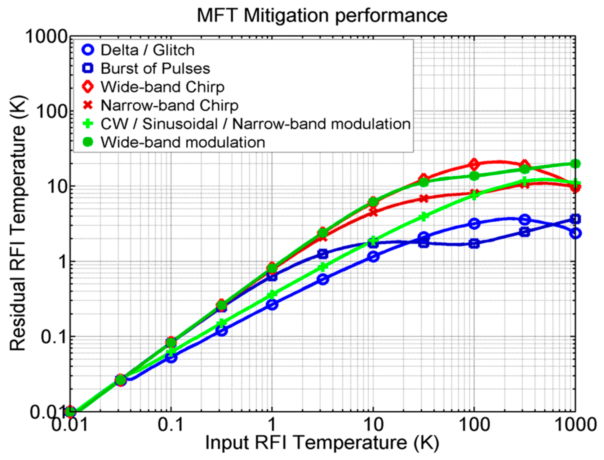
In [33], a novel method for D/M in the time, frequency, and scale domains, namely multiresolution Fourier transform (MFT), is presented as well, as a good tradeoff for all types of RFI. The results are shown in Figure 4.
The above techniques can or must be combined with two or more other domains in order to be as efficient as possible. As shown in Figure 3 and Figure 4, it is clear that to improve the overall RFI D/M performance a combination of different techniques must be included, notably the MFT, pulse blanking (for pulsed signals), and frequency blanking (for CW and narrowband signals). These can also be combined with statistical techniques (kurtosis and Anderson–Darling to avoid kurtosis blind spots [45]), and polarimetry techniques (measurement of the third and fourth Stokes parameters).
RFI D/M algorithms (usually) require real-time operation, which adds a new variable to take into account during the selection of the proper algorithm, i.e., the computational burden. It must be stated that all the above algorithms have been developed for real-aperture radiometers (or GNSS receivers) operating in real time, but, in principle, not for correlation radiometers (e.g., SMOS) that require the complex cross-correlation of two different signals. This brings another step of complexity as the signals to be correlated must be “cleaned” first, but some tests can be shared for all receivers in order to optimize the overall implementation.
3.2. Quantization and Sampling Effects
The impact of quantization and sampling has been studied in the literature separately. In [51], the impact of a general quantization scheme was expressed and analyzed as a nonlinear transformation.
It was found that, despite signal, quantization can significantly alter the value of the ideal cross-correlation (ρxy), it is possible to recover it from the measured one (Rxy) using then the function ρxy = q−1 [Rxy], which can always be computed numerically. Recall that signal power is equal to the autocorrelation value at the origin ρxx (0). In synthetic aperture radiometers (Section 4) the cross-correlation function ρxy(τ) is of outmost importance, and therefore it is very important to be able to recover the ideal correlation from the measured one for the particular quantization scheme used.
In [51] it was also found that there is an optimum configuration of the VADC/σx,y for each quantization scheme, that minimizes the correlation error. Additionally, quantization decreases the radiometric resolution, because it distorts and spreads the cross-correlation spectrum.
The spectrum of the cross-correlation function is also impacted by sampling, and depending on the sampling rate, replicas of the spectrum can overlap the main spectrum, even above the Nyquist criterion, due to spectrum spreading as a result of the nonlinear quantization process. This impacts the SNR, and therefore the radiometric resolution.
Finally, quantization and sampling were studied together to determine their impact on the variance of the measurements. Results showed that it strongly depends on the relationship between the bandwidth of the cross-correlation and the sampling rate. By increasing sampling rates, successive samples become more correlated, adding less new information, and therefore the variance decreases more slowly.
In [52], published in this Special Issue, the authors studied the impact of signal quantization on the performance of RFI mitigation algorithms. The one-bit quantization produces the strongest “clipping” of the amplitude signal, and the largest spectrum spreading. Since the amplitude information is lost, the instantaneous power information is also lost.
The optimum performance of mitigation algorithms is hampered by clipping because it affects the energy content of the signal, impairing RFI mitigation for large RFI powers. Pulse blanking is the exception to this, with a performance comparable to the unquantized case, even at high INR. Other mitigation algorithms, however, can only correct RFI up to an INR of ~6 to ~10 dB, and therefore clipping must be avoided as much as possible.
Automatic gain control systems are conceived to prevent clipping by adapting the input signal level to the dynamic range of the quantizer. However, since the number of bits is finite, as RFI power increases, quantization can no longer reproduce the radiometric signal itself, but only the RFI, degrading the performance of the mitigation technique. This effect, called ”underquantization”, strongly depends on the number of bits considered. Therefore, there is a tradeoff between system complexity and operating range of the RFI mitigation algorithms. ”Underquantization”, however, significantly degrades performance with respect to fixed VADC for three- and four-bit quantizers.
In addition, it has been demonstrated, due to clipping effects that are unavoidable using AGC systems, that one-bit quantization prevents using time and frequency mitigation methods, regardless of RFI power or other system parameters.
Figure 5, extracted [52], shows two spectrograms that illustrate the effect of spectrum spreading with one-bit quantization. In both cases, the RFI signal corresponds to a real-valued chirp-type RFI signal (symmetric with respect to the center of the frequency axis) with Gaussian band-limited noise. The vertical axis corresponds to digital frequency, the horizontal axis to samples, and the color scale is power in arbitrary dB. The first spectrogram approximates well to the ideal case (double precision in MATLAB), while the second spectrogram was obtained after the one-bit quantization of the signal. It can be observed how an RFI that could be located in the time-frequency space with certain precision is spread throughout the spectrum. It should be noted that temporary variations of power can be observed, but always after integration, therefore, the RFI signals that show fast pulsed power variations will be masked by the effect of quantization.
4. Review of RFI Detection and Mitigation Techniques in Synthetic Aperture Radiometers
The main differences between synthetic and real aperture radiometers are the following [53]:
- Real aperture radiometers refer to those that have a single antenna whose aperture determines how effective it is at receiving electromagnetic radiation power from a given direction. The antenna “effective area” is the physical area that intercepts the same amount of power from the wavefront.
- Synthetic aperture radiometers refer to those that use multiple small antennas and interferometric signal processing (basically the complex cross-correlation of the signals collected by each pair of antennas) to obtain the resolution of a single large antenna. The synthetic aperture approach overcomes the barriers that the physical size of the antenna places on passive microwave remote sensing from space, as it replaces an unrealistically large antenna with an array of small antennas, eventually even in different platforms.
Finally, both real and synthetic aperture radiometers can be fully polarimetric, or not. From the point of view of RFI D/M techniques, a synthetic aperture radiometer is seen, before the complex cross-correlations among all signal pairs are performed, as a collection of real aperture radiometers. As such, all the techniques listed above can be used. However, notably, the casuistic may be different as in a synthetic aperture radiometer the antennas have a modest directivity, and therefore, the received power from a given RFI source is smaller, although it will be “seen” during a longer period of time.
Cooperative detection approaches can also be implemented as basically the same RFI signal is collected by all antenna elements, as they are physically close, and within a maximum delay smaller than the coherence time (Tcoh ≈ 1/B, being B the noise bandwidth). For example, the simplest cooperative example may be applying pulse blanking; if an unusual large power is detected in one of the antennas, samples from all antennas are removed at the corresponding time.
However, although cooperative RFI mitigation can be applied in the simplest time, frequency, and statistical domain algorithms it is not feasible in other approaches or in a multi-domain approach. Therefore, the RFI mitigation must be applied to the signal received from each single antenna element before the cross-correlations are computed, otherwise it will contaminate all the cross-correlations pairs in which this contaminated signal is participating. It must be highlighted too that the dynamic range of the RFI signals that can be mitigated is strongly related to the number of bits used in the quantization process and the use, or not, of an AGC. For example, if the number of bits is low, and there is a strong RFI, the noise signal to be correlated is totally masked by the RFI, and either the correlation is that of the RFI signal, or if cleaned, the cross-correlation will be zero, as the noise signal will lie under the quantization noise.
Moreover, synthetic aperture radiometers allow for additional RFI mitigation techniques after correlation. If i and q are the in-phase and quadrature components of the received signals, subscripts 1 and 2 indicate the receivers’ numbers, and r and s indicate the polarization of the receiving antenna, the following properties must be satisfied if there is no RFI:
- and/or . This condition is satisfied by only Gaussian signals such as thermal noise.
- , for j = 1,2. This condition indicates that there are anomalously large third and fourth Stokes parameters either in the autocorrelation (j = 1) or in the cross-correlation (j = 2), whereas thermal emission from natural sources has a very small third Stokes parameter, and a negligible fourth Stokes one.
- must have the shape of the ideal fringe-washing function [53], if not, the inverse function used ρxy = q−1 [Rxy] is not performing.
- A last family of RFI D/M techniques can be applied after the image reconstruction process.
- An important and subtle difference between real and synthetic aperture radiometers, lies in the fact that the width of the synthetic solid angle of the synthetic aperture radiometer is much smaller than the antenna solid angles of each of the individual antennas forming the array. Therefore, when RFI signals are collected by the individual antennas of the synthetic aperture radiometer, the increase of the antenna temperature is much smaller than its real aperture antenna counterpart, and it is often hardly detected. Therefore, quantization and clipping effects are not as noticeable. For example, in the case of ESA SMOS mission, the individual antenna elements have an antenna beamwidth of ~70° [54], and in NASA SMAP mission ~2.7° [55]. Therefore, an RFI source producing a 1000 K antenna temperature increase in SMAP, would produce just a antenna temperature increase in SMOS individual antennas, as shown in Figure 3, which are hardly detectable and mitigable, except for pulsed or CW RFI signals.
Typically, the intensity of the RFI source only becomes visible after it is magnified during the image reconstruction process, and abnormal high brightness temperature spots appear in the synthetic image.
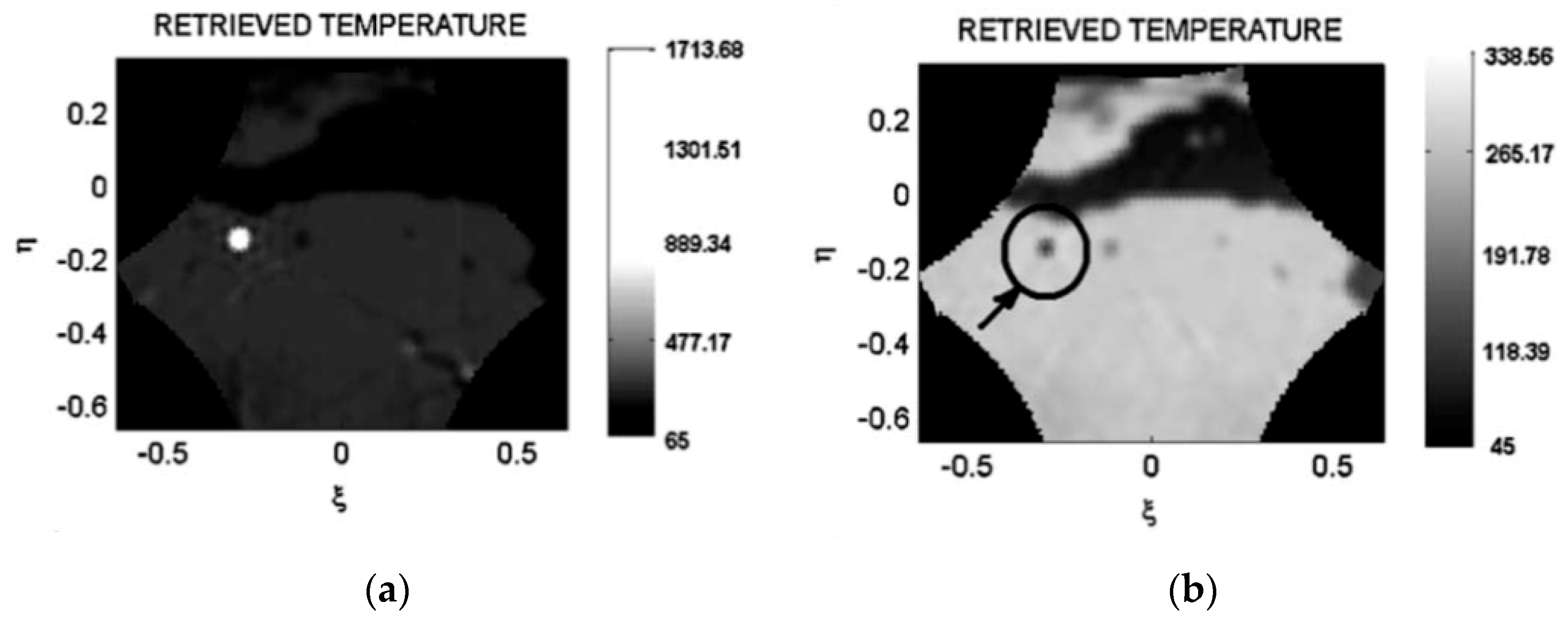
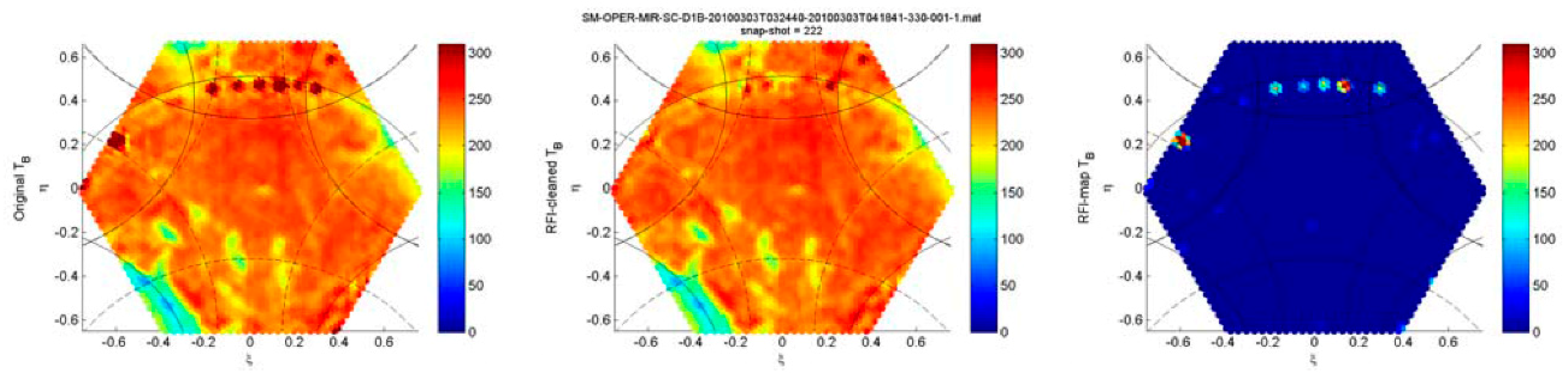
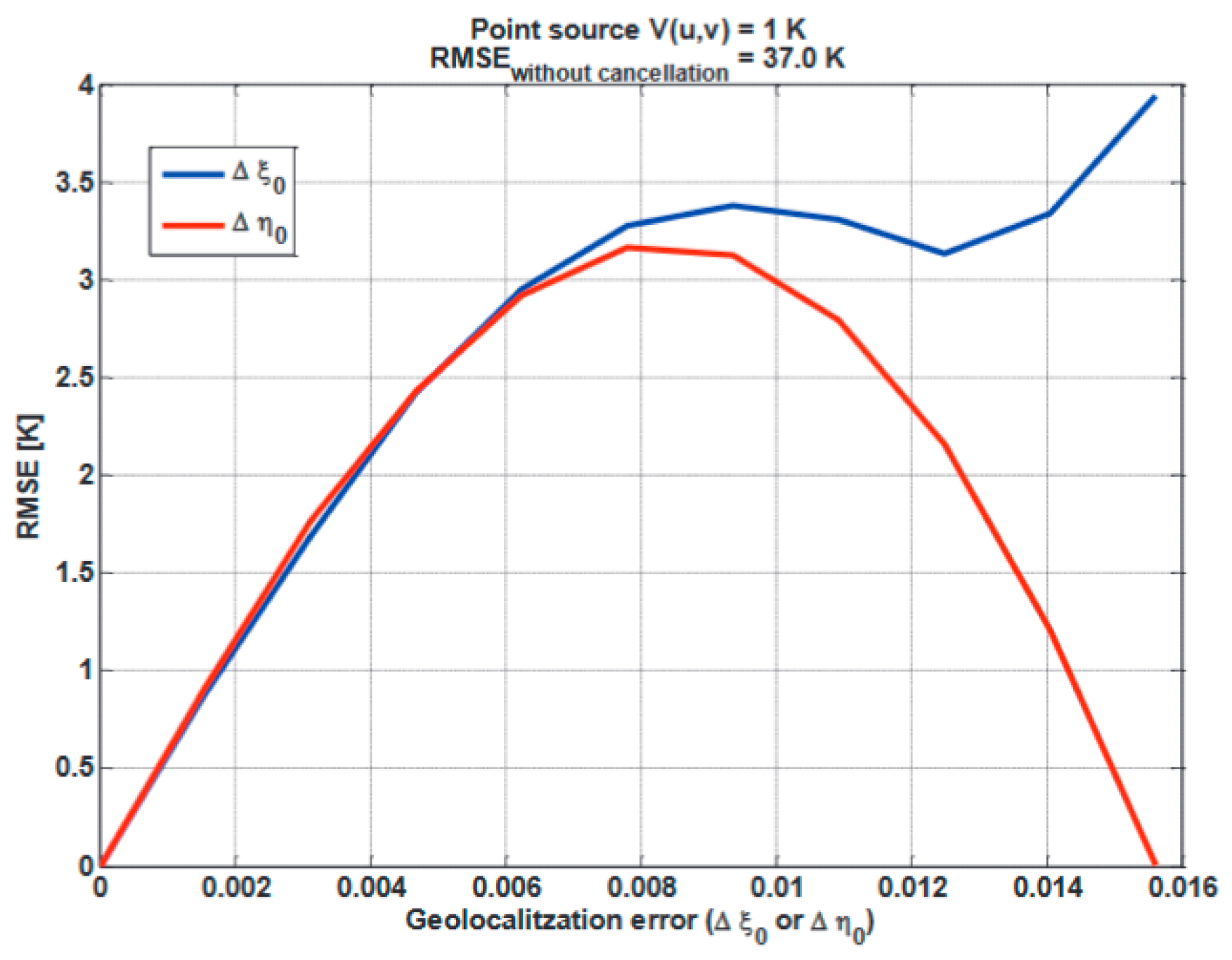
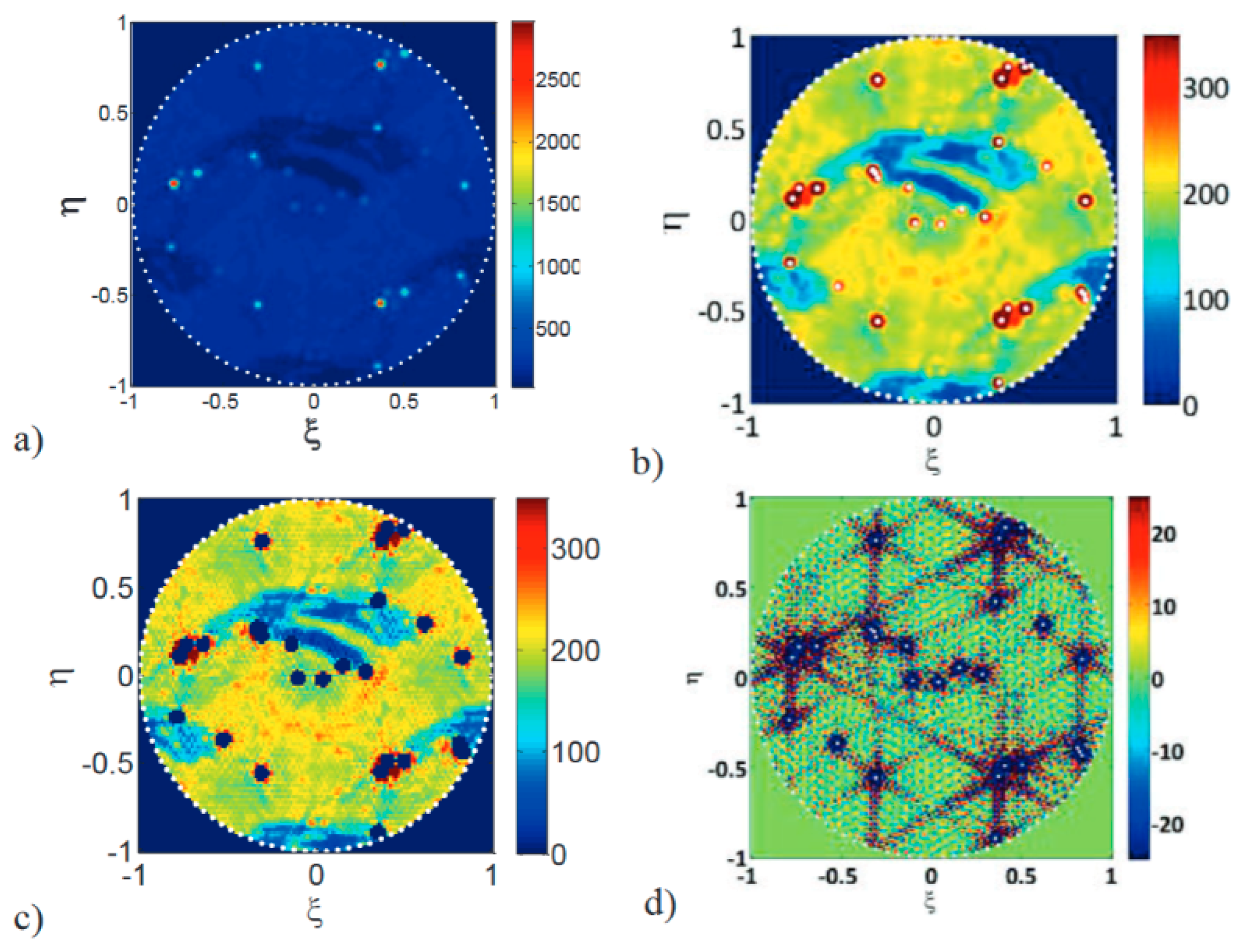
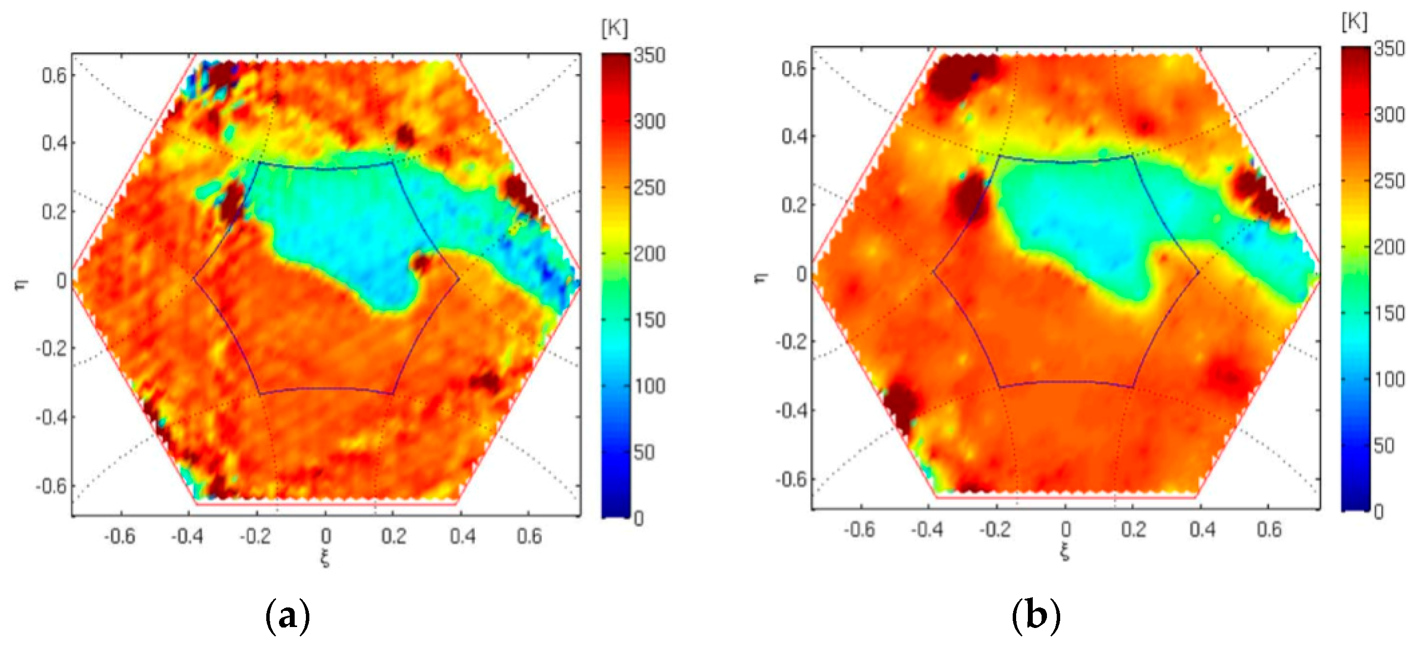
These last family of algorithms is based either on the detection of high brightness temperature values and subtracting the visibilities of an equivalent point source (e.g., Figure 6 [56]) or disk (Figure 7 [57]) at the same position and with an intensity such that the error is minimized (e.g., Figure 6); or on the formation of a synthetic beam that exhibits nulls in the directions of the RFI source (Figure 8 showing the residual error as a function of the geo-localization error and Figure 9 sample RFI mitigated SMOS imagery, both [58] or in more sophisticated methods that form the image over the pixels (“nodes”) that are less affected by RFI (Figure 10 [59]). In the first three cases, the whole radiometric information from those particular areas and most of the regions affected by the tails of the “impulse response” of the system is lost, while after mitigation, most of it becomes useful.
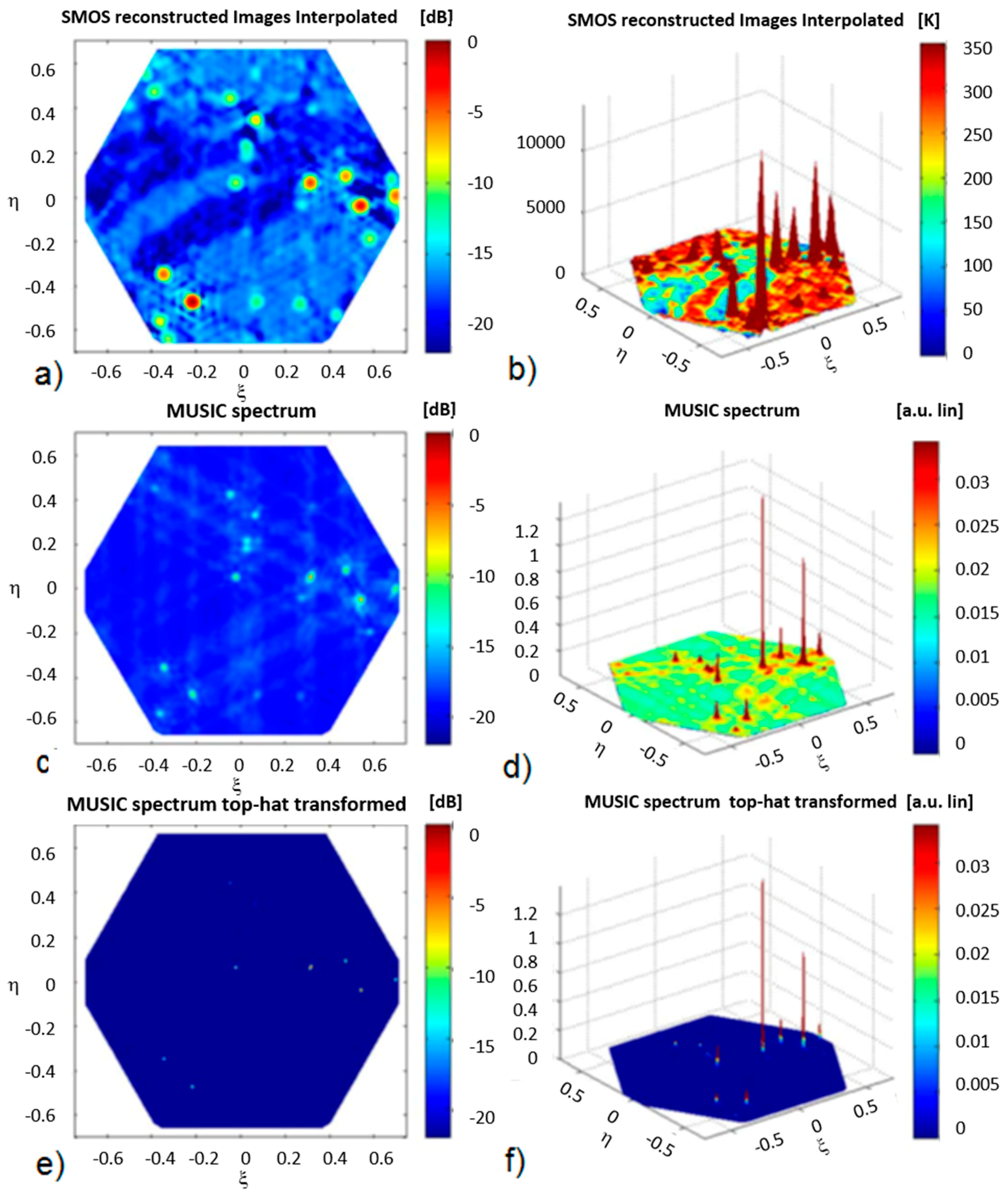
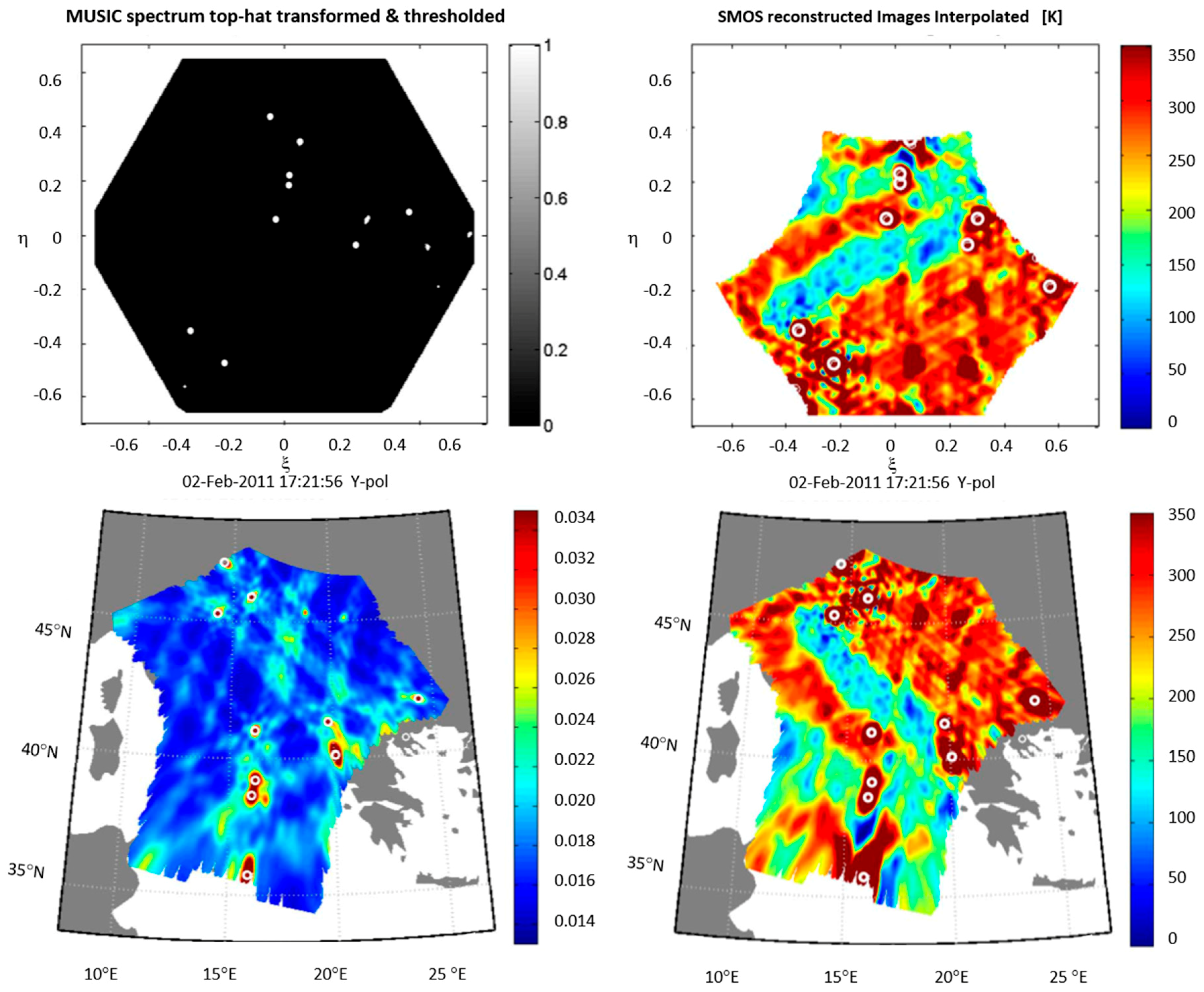
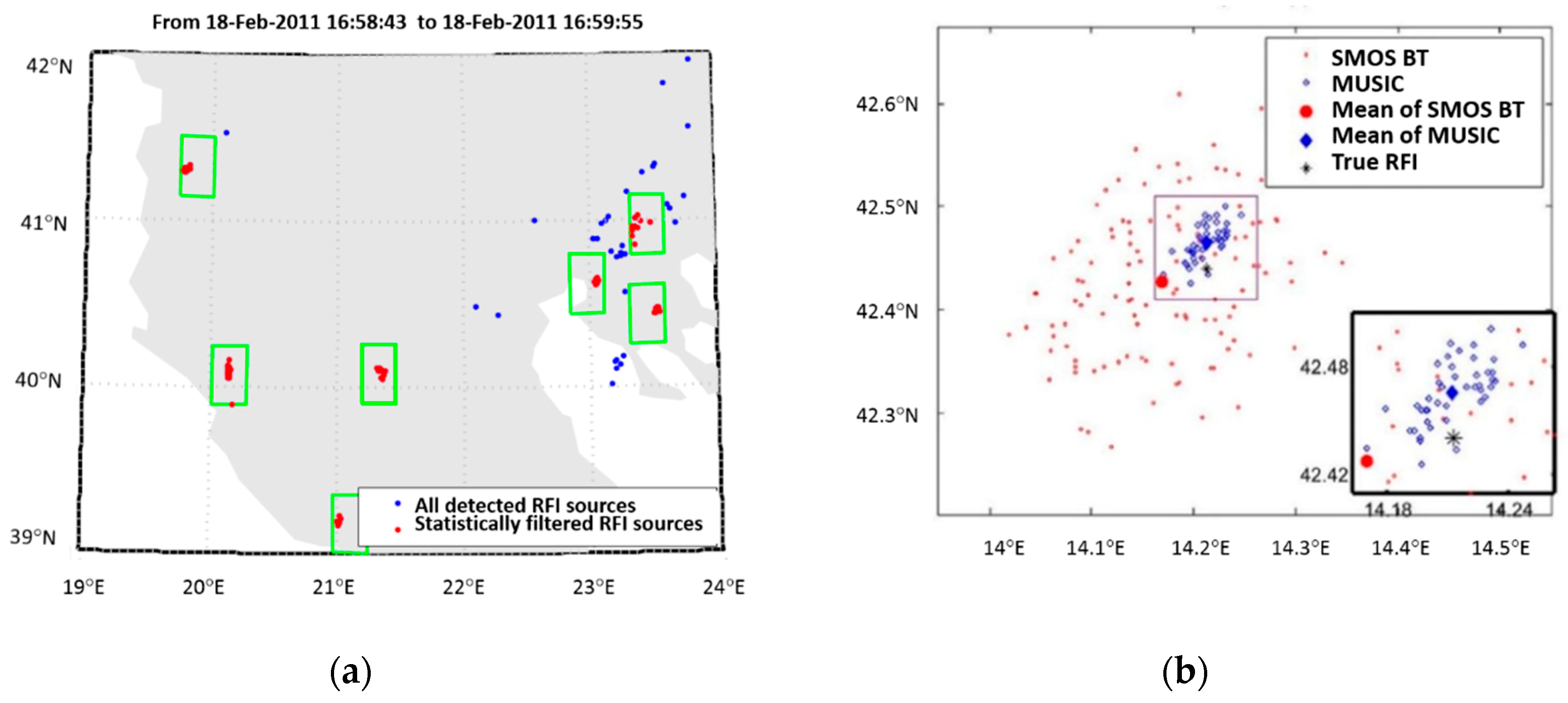
In addition, with an imaging instrument, RFI detection and localization (D/L) techniques (e.g., MUSIC algorithm [60]) can also be applied to achieve a higher geolocalization accuracy and input these positions in the above algorithms. The performance can be improved even further by averaging multiple observations derived with the MUSIC algorithm, achieving accuracies on the order of 1 to 2 km [60]. This process is illustrated in Figure 11, Figure 12 and Figure 13.
5. Discussion on Synthetic Aperture Radiometers RFI Detection and Mitigation
So far, SMOS has been the only synthetic aperture radiometer onboard a satellite mission. Due to the large number of correlators only one-bit (two levels) correlators can be implemented, and this is even more true for planned missions with even a larger number of antenna elements and correlators.
However, as mentioned before, the one-bit quantization makes the RFI detection/mitigation more difficult. At some point, it can completely prevent removal of the RFI power out of the desired radiometric noise. A better scenario would be to apply the mitigation algorithm to a quantized signal with multiple bits, and then quantize the already mitigated signal to one bit. However, if the one-bit quantization scheme is immovable, then the alternatives that can be applied to mitigate the RFI signal at different stages are the following:
Using the power measurement system or PMS (diode detector in each receiver, acting as a total power radiometer, which is required to denormalize the cross-correlations computed at one bit):
- Mitigation with pulse blanking involves removing samples when the power is above a certain threshold. Fast pulses are not detected if the integration time is too long, but it must be adjusted to respond to arbitrary short pulses, at the expense of a larger noise, i.e., and increased false alarm rate. In any case, averaging of the RFI-free detected voltages is advisable to recover radiometric sensitivity.
- Detection with kurtosis and/or exponential test analyzes if the PMS signal contains signals that are not Gaussian.
At signal before the correlator quantized to one bit:
- Mitigation with frequency blanking or spectrogram blanking eliminates parts of the spectrum where more RFI power is concentrated. The performance is degraded with respect to the multibit case by the spectrum broadening (e.g., Figure 5).
- Detection with spectral kurtosis is the same principle as in the case of the PMS signal, with the same limitations as in the previous case.
- Multiple antenna outputs could, in principle, be used to reduce noise and improve the estimates. However, taking into account that the antenna noise is highly correlated, and only the receivers’ noise is uncorrelated from one antenna element to another one, the variance reduction due to averaging does not decrease as 1/N.
After correlator, the RFI signal cannot be mitigated any more.
- RFI can be detected by analyzing the third and fourth Stokes parameters. A polarimetric analysis detects if the radiometric signal is contaminated by RFI, but only data frames as a whole are discarded.
- The use of multiple antenna outputs. After image formation, several algorithms [56,57,58,59] have been developed to mitigate the RFI sources during the image formation process. To do that most effectively, the geolocation of the RFI sources must be known beforehand. To achieve this, repeated-pass MUSIC-based algorithms have been developed achieving accuracies in the order of 1 to 2 km [60].
6. Conclusions
This paper has reviewed the different techniques to detect and mitigate RFI in real and synthetic aperture microwave radiometers. Since there is no single technique that copes with all types of RFI sources, a combination of different techniques must be used to effectively protect against RFI. Currently, these techniques are more mature in real aperture radiometers, and after the NASA SMAP mission, most microwave radiometry missions which include bands under K-band are incorporating some of these algorithms. Synthetic aperture radiometers are younger and less mature. However, after SMOS sufferings from RFI, a number of techniques have been reviewed, new ones have been proposed (Section 4), and detection/mitigation techniques after the image reconstruction process have all been reviewed together because the accuracy of the mitigation relies on accurate RFI geolocation, in which MUSIC-type algorithms outperform. Finally, the limitations introduced by the use of one bit and level two samples are discussed, and although a multi-bit sampling scheme would be beneficial, RFI detection and mitigation at one bit and level two is still feasible.
Author Contributions
Conceptualization, J.Q. and A.C.; methodology, J.Q. and A.C.; software, J.Q.; validation, J.Q., A.P., and A.C.; formal analysis, J.Q and A.C.; investigation, A.C.; resources, J.Q. and A.C.; data curation, J.Q. and A.P.; writing—original draft preparation, J.Q. and A.C.; writing—review and editing, J.Q., A.P., and A.C.; visualization, J.Q.; supervision, A.C.; project administration, A.C.; funding acquisition, A.C.
Funding
This work is partially funded by ICREA under the ICREA Academia programme (award Prof. A. Camps), by the Spanish Ministry MINECO and EU ERDF project (RTI2018-099008-B-C21) “Sensing with pioneering opportunistic techniques”, by “CommSensLab” Excellence Research Unit Maria de Maeztu, and by ESA project EOP-ΦMM/2018-03-2072/MS/ms.
Conflicts of Interest
The authors declare no conflict of interest.
References
- Gasiewski, A.; Klein, M.; Yevgrafov, A.; Leuskiy, V. Interference mitigation in passive microwave radiometry. In Proceedings of the IEEE International Geoscience and Remote Sensing Symposium, Toronto, ON, Canada, 24–28 June 2002; pp. 1682–1684. [Google Scholar]
- Ulaby, F.T.; Moore, R.K.; Fung, A.K. Microwave Remote Sensing: Active and Passive. In Microwave Remote Sensing Fundamentals and Radiometry; Artech House Publishers: Norwood, MA, USA, 1981; Volume 1. [Google Scholar]
- Querol, J.; Onrubia, R.; Pascual, D.; Alonso-Arroyo, A.; Park, H.; Camps, A. Comparison of real-time time-frequency RFI mitigation techniques in microwave radiometry. In Proceedings of the 2016 14th Specialist Meeting on Microwave Radiometry and Remote Sensing of the Environment (MicroRad), Espoo, Finland, 11–14 April 2016; pp. 68–70. [Google Scholar]
- Njoku, E.; Ashcroft, P.; Chan, T.; Li, L. Global survey and statistics of radio-frequency interference in AMSR-E land observation. IEEE Trans. Geosci. Remote Sens. 2005, 43, 938–947. [Google Scholar] [CrossRef]
- Ellingson, S.W.; Johnson, J.T. A polarimetric Survey of Radio Frequency Interference in C and X bands in the Continental United States using WindSat Radiometry. IEEE Trans. Geosci. Remote Sens. 2006, 44, 540–548. [Google Scholar] [CrossRef]
- Draped, D.W.; de Matthaeis, P. Characteristics of 18.7 GHZ Reflected Radio Frequency Interference in Passive Radiometer Data. In Proceedings of the IGARSS 2019—2019 IEEE International Geoscience and Remote Sensing Symposium, Yokohama, Japan, 28 July–2 August 2019; pp. 4459–4462. [Google Scholar]
- Dente, L.; Su, Z.; Wen, J. Validation of SMOS Soil Moisture Products over the Maqu and Twente Regions. Sensors 2012, 12, 9965–9986. [Google Scholar] [CrossRef] [PubMed]
- Li, L.; Njoku, E.; Im, E.; Chang, P.; St.Germain, K. A Preliminary Survey of Radio-Frequency Interference Over the U.S. in Aqua AMSRE Data. IEEE Trans. Geosci. Remote Sens. 2004, 42, 380–390. [Google Scholar] [CrossRef]
- Soldo, Y.; Khazaal, A.; Cabot, F.; Kerr, Y.H. An RFI Index to Quantify the Contamination of SMOS Data by Radio-Frequency Interference. IEEE J. Sel. Top. Appl. Earth Obs. Remote Sens. 2016, 9, 1577–1589. [Google Scholar] [CrossRef]
- Mohammed, P.N.; Aksoy, M.; Piepmeier, J.R.; Johnson, J.T.; Bringer, A. SMAP L-Band Microwave Radiometer: RFI Mitigation Prelaunch Analysis and First Year On-Orbit Observations. IEEE Trans. Geosci. Remote Sens. 2016, 54, 6035–6047. [Google Scholar] [CrossRef]
- Misra, S.; de Matthaeis, P. Passive Remote Sensing and Radio Frequency Interference (RFI): An Overview of Spectrum Allocations and RFI Management Algorithms [Technical Committees]. IEEE Geosci. Remote Sens. Mag. 2014, 2, 68–73. [Google Scholar] [CrossRef]
- Landry, R.J.; Boutin, P.; Constantinescu, A. New anti-jamming technique for GPS and GALILEO receivers using adaptive FADP filter. Digit. Signal Process. A Rev. J. 2006, 16, 255–274. [Google Scholar] [CrossRef]
- Tarongi, J.M.; Camps, A. Radio frequency interference detection and mitigation algorithms based on spectrogram analysis. Algorithms 2011, 4, 239–261. [Google Scholar] [CrossRef] [Green Version]
- Antoni, J. The spectral kurtosis: A useful tool for characterizing non-stationary signals. Mech. Syst. Signal Process. 2006, 20, 282–307. [Google Scholar] [CrossRef]
- Camps, A.; Tarongi, J.M. RFI Mitigation in Microwave Radiometry Using Wavelets. Algorithms 2009, 2, 1248–1262. [Google Scholar] [CrossRef] [Green Version]
- Querol Borràs, J. Radio Frequency Interference Detection and Mitigation Techniques for Navigation and Earth Observation. Ph.D. Thesis, Universitat Politècnica de Catalunya-BarcelonaTech, Barcelona, Spain, November 2018. Available online: http://hdl.handle.net/10803/663905 (accessed on 15 September 2019).
- Getu, T.M.; Ajib, W.; Landry, R. An Eigenvalue-Based Multi-Antenna RFI Detection Algorithm. In Proceedings of the 2018 IEEE 88th Vehicular Technology Conference (VTC-Fall), Chicago, IL, USA, 27–30 August 2018; pp. 1–5. [Google Scholar]
- Nguyen, L.H.; Tran, T.D. A comprehensive performance comparison of RFI mitigation techniques for UWB radar signals. In Proceedings of the 2017 IEEE International Conference on Acoustics, Speech and Signal Processing (ICASSP), New Orleans, LA, USA, 5–9 March 2017; pp. 3086–3090. [Google Scholar]
- Abdelhadi, K.A.; Clancy, T.C. Spectrum Sharing Between Radars and Communication Systems: A MATLAB Based Approach; Chapter 3.2; Springer: New York, NY, USA, 12 June 2017. [Google Scholar]
- Schoenwald, A.J.; Gholian, A.; Bradley, D.C.; Wong, M.; Mohammed, P.N.; Piepmeier, J.R. RFI detection and mitigation using independent component analysis as a pre-processor. In Proceedings of the 2016 Radio Frequency Interference (RFI), Socorro, NM, USA, 17–20 October 2016; pp. 100–104. [Google Scholar]
- Kay, S.M. Fundamentals of Statistical Signal Processing: Detection theory; Prentice-Hall PTR: Englewood Cliffs, NJ, USA, 1993. [Google Scholar]
- Kandangath, A. Jamming Mitigation Techniques for Spread Spectrum Communication Systems. Signal Process. Wirel. Commun. 2003. [Google Scholar]
- Baan, W.A. RFI mitigation in radio astronomy. In Proceedings of the 2011 30th URSI General Assembly and Scientific Symposium (URSIGASS), Istanbul, Turkey, 13–20 August 2011. [Google Scholar]
- Tarongí, J.M. Radio Frequency Interference in Microwave Radiometry: Statistical Analysis and Study of Techniques for Detection and Mitigation. Ph.D. Thesis, Universitat Politècnica de Catalunya-BarcelonaTech, Barcelona, Spain, March 2012. Available online: https://www.tdx.cat/handle/10803/117023 (accessed on 12 September 2019).
- Forte Véliz, G.F. Contributions to Radio Frequency Interference Detection and Mitigation in Earth Observation. Ph.D. Thesis, Universitat Politècnica de Catalunya-BarcelonaTech, Barcelona, Spain, June 2013. Available online: https://www.tdx.cat/handle/10803/285320 (accessed on 12 September 2019).
- Oppenheim, A.V.; Schafer, R.W.; Buck, J.R. Discrete Time Signal Processing, 3rd ed.; Pearson Education, Limited: London, UK, 1999. [Google Scholar]
- Manolakis, D.G.; Ingle, V.K.; Kogon, S.M. Statistical and Adaptive Signal Processing: Spectral Estimation, Signal Modeling, Adaptive Filtering, and Array Processing; Artech House: Norwood, MA, USA, 2000. [Google Scholar]
- Borio, D.; O’Driscoll, C.; Fortuny, J. GNSS jammers: Effects and countermeasures. In Proceedings of the 6th ESA Workshop on Satellite Navigation Technologies: Multi-GNSS Navigation Technologies Galileo’s Here, NAVITEC 2012 and European Workshop on GNSS Signals and Signal Processing, Noordwijk, The Netherlands, 5–7 December 2012. [Google Scholar]
- Borio, D.; O’driscoll, C.; Fortuny, J. Tracking and Mitigating a Jamming Signal with an Adaptive Notch Filter. InsideGNSS, March–April 2014; 67–73. [Google Scholar]
- Borio, D.; Camoriano, L.; Presti, L.L. Two-Pole and Multi-Pole Notch Filters: A Computationally Effective Solution for GNSS Interference Detection and Mitigation. IEEE Syst. J. 2008, 2, 38–47. [Google Scholar] [CrossRef]
- Hall, M. Resolution and uncertainty in spectral decomposition. First Break 2006, 24, 43–47. [Google Scholar] [CrossRef]
- Rifkin, R.; Vaccaro, J.J. Comparison of narrowband adaptive filter technologies for GPS. In Proceedings of the 2000 IEEE Position Location and Navigation Symposium, San Diego, SA, USA, 13–16 March 2000. [Google Scholar]
- Querol, J.; Onrubia, R.; Alonso-Arroyo, A.; Pascual, D.; Park, H.; Camps, A. Performance Assessment of Time–Frequency RFI Mitigation Techniques in Microwave Radiometry. IEEE J. Sel. Top. Appl. Earth Obs. Remote Sens. 2017, 10, 3096–3106. [Google Scholar] [CrossRef]
- Ruf, C.S.; Gross, S.M.; Misra, S. RFI detection and mitigation for microwave radiometry with an agile digital detector. IEEE Trans. Geosci. Remote Sens. 2006, 44, 694–706. [Google Scholar] [CrossRef]
- Akansu, A.N.; Haddad, R.A. Multiresolution Signal Decomposition: Transforms, Subbands, and Wavelets; Academic Press Elsevier Science: Cambridge, MA, USA, 2001. [Google Scholar]
- Chakraborty, D.; Kovvali, N. Generalized normal window for digital signal processing. In Proceedings of the 2013 IEEE International Conference on Acoustics, Speech and Signal Processing (ICASSP), Vancouver, BC, Canada, 26–31 May 2013; pp. 6083–6087. [Google Scholar]
- Starosielec, S.; Hägele, D. Discrete-time windows with minimal RMS bandwidth for given RMS temporal width. Signal Process. 2014, 102, 240–246. [Google Scholar] [CrossRef]
- Mallat, S.; Wavelet, A. Tour of Signal Processing: The Sparse Way, 3rd ed.; Academic Press Elsevier Science: Cambridge, MA, USA, 1999. [Google Scholar]
- Forte, G.; Querol, J.; Park, H.; Camps, A. Digital back-end for RFI detection and mitigation in earth observation. In Proceedings of the 2013 IEEE International Geoscience and Remote Sensing Symposium—IGARSS, Melbourne, VIC, Australia, 21–26 July 2013; pp. 1908–1911. [Google Scholar]
- Musumeci, L.; Dovis, F. Use of the Wavelet Transform for Interference Detection and Mitigation in Global Navigation Satellite Systems. Int. J. Navig. Obs. 2014, 2014. [Google Scholar] [CrossRef]
- Maccone, C. Mathematical SETI: Statistics, Signal Processing, Space Missions; Springer Berlin Heidelberg: Berlin/Heidelberg, Germany, 2010. [Google Scholar]
- Szumski, A.; Hein, G.W. Finding the Interference: Karhunen-Loève Transform as an instrument to Detect Weak RF signals. InsideGNSS, May–June 2011; 57–64. [Google Scholar]
- Yu, W.; Deng, Y.; Wang, X.; Qi, X.; Liu, Y. Radiofrequency interference suppression in synthetic aperture radar based on singular spectrum analysis with extended—FAPI subspace tracking. IET Radar Sonar Navig. 2012, 6, 881–890. [Google Scholar]
- Trinkle, M.; Gray, D. GPS interference mitigation; overview and experimental results. In Proceedings of the 2001 5th International Symposium on Satellite Navigation Technology and Applications (SatNav), Canberra, Australia, 24–27 July 2001. [Google Scholar]
- Tarongi, J.M.; Camps, A. Normality Analysis for RFI Detection in Microwave Radiometry. Remote Sens. 2010, 2, 191–210. [Google Scholar] [CrossRef] [Green Version]
- de Roo, R.D.; Misra, S.; Ruf, C.S. Sensitivity of the Kurtosis Statistic as a Detector of Pulsed Sinusoidal RFI. IEEE Trans. Geosci. Remote Sens. 2007, 45, 1938–1946. [Google Scholar] [CrossRef] [Green Version]
- Querol Borràs, J. Implementation of Radio-Frequency Interference Detection and Mitigation Algorithms for Communications and Navigation. Master’s Thesis, Universitat Politècnica de Catalunya-BarcelonaTech, Barcelona, Spain, November 2013. [Google Scholar]
- Taylor, J.; Denman, N.; Bandura, K.; Berger, P.; Masui, K.; Renard, A.; Tretyakov, I.; Vanderlinde, K. Spectral Kurtosis-Based RFI Mitigation for CHIME. J. Astron. Instrum. 2019, 8, 1940004. [Google Scholar] [CrossRef]
- GAJT. Novatel. Available online: https://www.novatel.com/products/gnss-antennas/gajt-anti-jam-antennas/gajt/ (accessed on 15 September 2019).
- Lundberg, E.; McMichael, I. Novel Timing Antennas for Improved GNSS Resilience; MITRE Technical Papers; MITRE: Bedford, MA, USA, March 2018. [Google Scholar]
- Bosch-Lluis, X.; Ramos-Perez, I.; Camps, A.; Rodriguez-Alvarez, A.; Valencia, E.; Park, H. A General Analysis of the Impact of Digitization in Microwave Correlation Radiometers. Sensors 2011, 11, 6066–6087. [Google Scholar] [CrossRef] [PubMed] [Green Version]
- Díez-García, R.; Camps, A. Impact of Signal Quantization on the Performance of RFI Mitigation Algorithms. Remote Sens. 2019, 11, 2023. [Google Scholar] [CrossRef] [Green Version]
- Camps, A.; Swift, C.T. New Techniques in Microwave Radiometry for Earth Remote Sensing; URSI Review of Radio Science 1999-2002; Ross Stone, W., Ed.; International Union of Radio Science by the IEEE-Press and Wiley-Interscience: Hoboken, NJ, USA, 2002; pp. 499–518. [Google Scholar]
- SMOS (Soil Moisture and Ocean Salinity) Mission. Available online: https://directory.eoportal.org/web/eoportal/satellite-missions/s/smos (accessed on 3 December 2019).
- SMAP (Soil Moisture Active/Passive) Mission. Available online: https://directory.eoportal.org/web/eoportal/satellite-missions/s/smap (accessed on 3 December 2019).
- Camps, A.; Vall-llossera, M.; Duffo, N.; Zapata, M.; Corbella, I.; Torres, F.; Barrena, V. Sun effects in 2-D aperture synthesis radiometry imaging and their cancelation. IEEE Trans. Geosci. Remote Sens. 2004, 42, 1161–1167. [Google Scholar] [CrossRef]
- Camps, A.; Gourrion, J.; Tarongi, J.M.; Llossera, M.V.; Gutierrez, A.; Barbosa, J.; Castro, R. Radio-requency Interference Detection and Mitigation Algorithms for Synthetic Aperture Radiometers. Algorithms 2011, 4, 155–182. [Google Scholar] [CrossRef] [Green Version]
- Camps, A.; Park, H.; Gonzalez-Gambau, V. An imaging algorithm for synthetic aperture interferometric radiometers with built-in RFI mitigation. In Proceedings of the 2014 13th Specialist Meeting on Microwave Radiometry and Remote Sensing of the Environment (MicroRad), Pasadena, CA, USA, 20–27 March 2014; pp. 39–43. [Google Scholar] [CrossRef]
- González-Gambau, V.; Turiel, A.; Olmedo, E.; Martínez, J.; Corbella, I.; Camps, A. Nodal Sampling: A New Image Reconstruction Algorithm for SMOS. IEEE Trans. Geosci. Remote Sens. 2016, 54, 2314–2328. [Google Scholar] [CrossRef] [Green Version]
- Park, H.; González-Gambau, V.; Camps, A.; Vall-llossera, M. Improved MUSIC-Based SMOS RFI Source Detection and Geolocation Algorithm. IEEE Trans. Geosci. Remote Sens. 2016, 54, 1311–1322. [Google Scholar] [CrossRef] [Green Version]
Figure 1.
A five-dimensional Venn diagram illustrating the different classes of radio frequency interference (RFI) detection and mitigation algorithms and their combinations. Two (red), three (blue), four (green), and five (grey) class combinations are possible. The algorithms from top to bottom correspond to: (top-left) pulse detection (temporal), (top-right) 3rd/4th Stokes RFI detection (polarimetric), (middle-left and middle-right) spectrogram (temporal + spectral) and (bottom-center), spectral kurtosis (temporal + spectral + statistical). Figure extracted from [11].
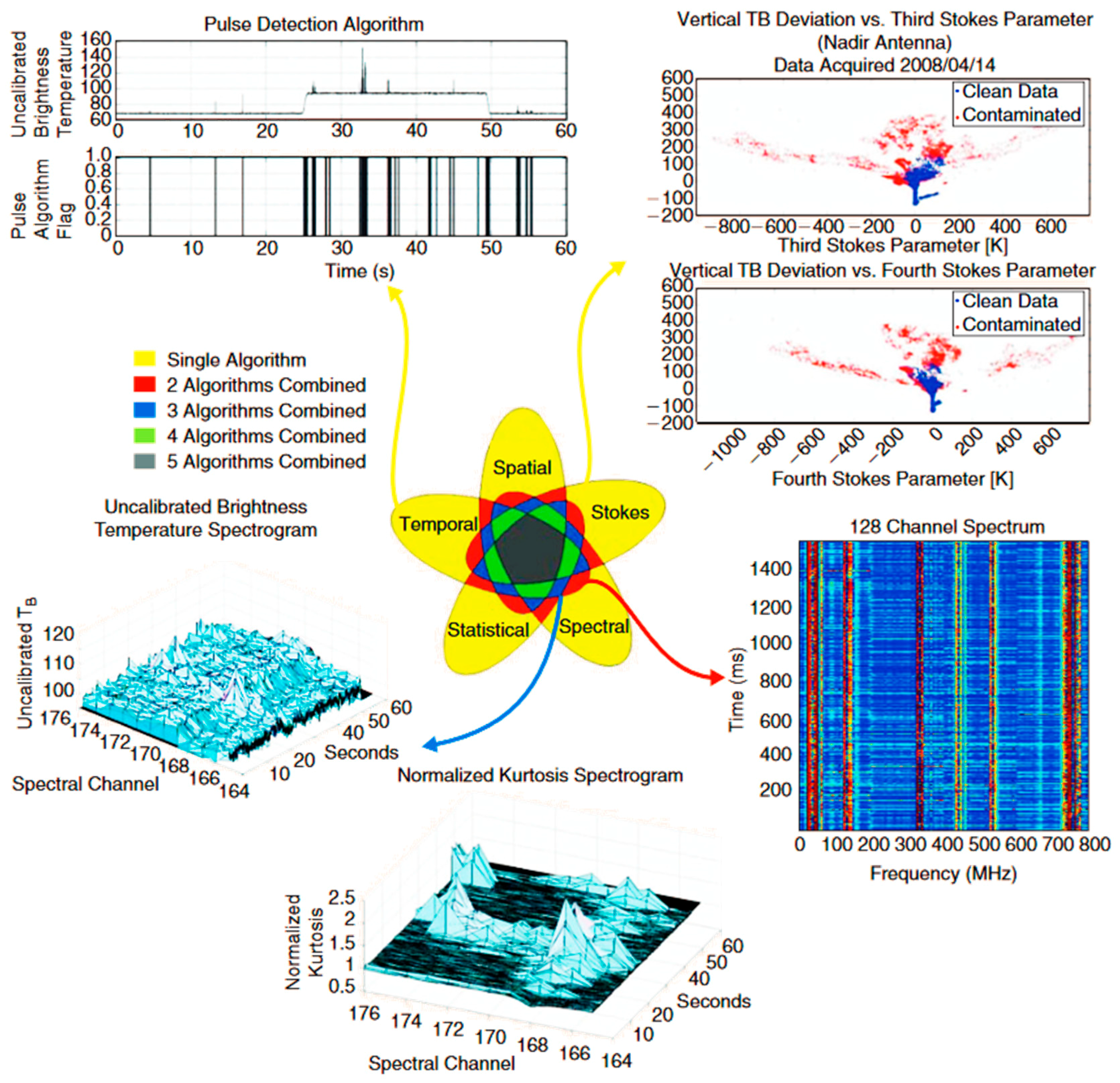
Figure 2.
Allocation in the time-frequency space of the mentioned groups of detection and mitigation techniques: (a) Time, (b) frequency, (c) time-frequency space domains, and (d) wavelets.
Figure 2.
Allocation in the time-frequency space of the mentioned groups of detection and mitigation techniques: (a) Time, (b) frequency, (c) time-frequency space domains, and (d) wavelets.
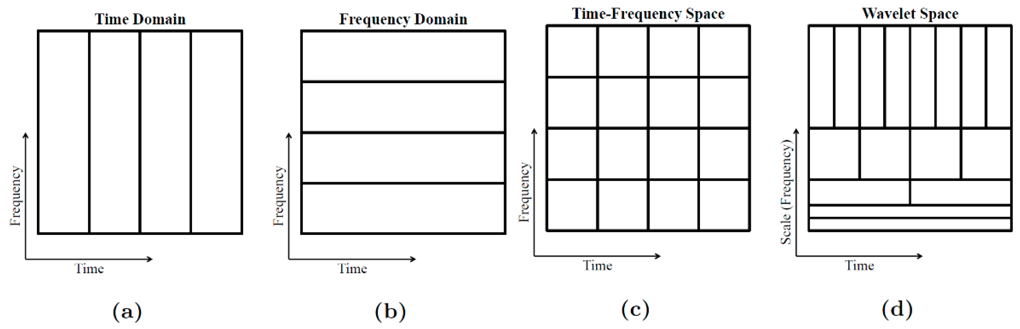
Figure 3.
Optimum mitigation performance of different RFI mitigation techniques for each type of RFI (extracted from [33]).
Figure 3.
Optimum mitigation performance of different RFI mitigation techniques for each type of RFI (extracted from [33]).

Figure 4.
Multiresolution Fourier transform (MFT) mitigation performance for different types of RFI signals (extracted from [33]).
Figure 4.
Multiresolution Fourier transform (MFT) mitigation performance for different types of RFI signals (extracted from [33]).

Figure 5.
Spectrogram of 300 K RMS noise signal contaminated by an RFI chirp of 15,000 K. (a) Before quantization and (b) after 1-bit quantization [52].
Figure 5.
Spectrogram of 300 K RMS noise signal contaminated by an RFI chirp of 15,000 K. (a) Before quantization and (b) after 1-bit quantization [52].

Figure 6.
(a) Reconstructed brightness temperature in the extended Alias-Free Field of View (AF-FOV) with Sun/moon effects, and (b) after Sun cancelation (from Figure 4 of [56]).
Figure 6.
(a) Reconstructed brightness temperature in the extended Alias-Free Field of View (AF-FOV) with Sun/moon effects, and (b) after Sun cancelation (from Figure 4 of [56]).

Figure 7.
RFI detection and mitigation algorithm performance: (left) SMOS dual-pol L1b image with RFI, (center) SMOS RFI-cleaned L1b image, and (right) detected RFI map. Most RFI sources are attenuated despite there are some not completely removed or as in (center) they have been over-compensated (from Figure 13a of [57]).

Figure 8.
Residual root mean squared error (RMSE) after RFI mitigation, for an RFI source at the origin, with an estimated position in the ξ (blue) and η (red) directions. Δξ = 2/128. RMSE without mitigation = 37.0 K (from Figure 5 of [58]).
Figure 8.
Residual root mean squared error (RMSE) after RFI mitigation, for an RFI source at the origin, with an estimated position in the ξ (blue) and η (red) directions. Δξ = 2/128. RMSE without mitigation = 37.0 K (from Figure 5 of [58]).

Figure 9.
Sample (a) SMOS brightness temperature (BT) scene over Central Europe contaminated by RFI, (b) same as (a), but with adjusted color scale, (c) same as (a), but with RFI mitigated, and (d) difference between (b) and (c). (from Figure 6 of [58]).
Figure 9.
Sample (a) SMOS brightness temperature (BT) scene over Central Europe contaminated by RFI, (b) same as (a), but with adjusted color scale, (c) same as (a), but with RFI mitigated, and (d) difference between (b) and (c). (from Figure 6 of [58]).

Figure 10.
(a) Sample RFI contaminated nominal BT image and (b) retrieved BT after applying nodal sampling technique, using an oversampling factor β = 9 (from Figure 6 of [59]).
Figure 10.
(a) Sample RFI contaminated nominal BT image and (b) retrieved BT after applying nodal sampling technique, using an oversampling factor β = 9 (from Figure 6 of [59]).

Figure 11.
First row: SMOS BT images (a and b). Second row: MUSIC spectrum estimated from same visibility samples (c and d). Third row: MUSIC spectrum after top-hat transform (e and f). To increase the contrast, first column shows normalized and log-scaled values (a,c,e), i.e., spectra in dB. Second column shows a three-dimensional view of spectra in linear scale (b,d,f) (from Figure 4 of [60]).

Figure 12.
(a) Detected RFI sources after thresholding the top-hat-transformed MUSIC spectrum (antenna reference frame, fundamental hexagon). (b) Detected RFI sources overlaid on the SMOS BT map (director cosines domain truncated to extended alias-free field-of-view). Georeferenced RFI sources superimposed on (c) MUSIC spectrum, and (d) SMOS BT map. White circles indicate locations of RFI sources detected by MUSIC (from Figure 5 of [60]).

Figure 13.
(a) Sample multiple-snapshot processing. Blue and red dots denote all RFI spots and selected ones, respectively. Selected bins depicted by green boxes. Bin size of 20 km × 20 km and a hit rate of 30% used (from Figure 6 of [56]). (b) Sample results for RFI source detection using SMOS BT maps, multiple-snapshot processing using three different overpasses, and true location of RFI source #14 (from Figure 8 of [60]).


Table 1.
Microwave radiometer sensitivity requirements for some typical applications [2,3]. Final application requirements may vary case by case.
| Application | Sensitivity | Application | Sensitivity |
|---|---|---|---|
| Atmospheric temperature profile | 0.3 K | Atmospheric water vapor profile | 0.5 K |
| Cloud liquid water content | 1 K | Sea surface temperature | 0.3 K |
| Sea surface salinity | 0.3 K | Sea wind speed | 1 K |
| Sea ice concentration | 2 K | Ice mapping | 1 K |
| Rain rate | 0.5 K | Oil slicks | 0.3 K |
| Soil moisture | 1 K | Snow cover | 1 K |
© 2019 by the authors. Licensee MDPI, Basel, Switzerland. This article is an open access article distributed under the terms and conditions of the Creative Commons Attribution (CC BY) license (http://creativecommons.org/licenses/by/4.0/).
Share and Cite
MDPI and ACS Style
Querol, J.; Perez, A.; Camps, A. A Review of RFI Mitigation Techniques in Microwave Radiometry. Remote Sens. 2019, 11, 3042. https://0-doi-org.brum.beds.ac.uk/10.3390/rs11243042
AMA Style
Querol J, Perez A, Camps A. A Review of RFI Mitigation Techniques in Microwave Radiometry. Remote Sensing. 2019; 11(24):3042. https://0-doi-org.brum.beds.ac.uk/10.3390/rs11243042
Chicago/Turabian StyleQuerol, J., A. Perez, and A. Camps. 2019. "A Review of RFI Mitigation Techniques in Microwave Radiometry" Remote Sensing 11, no. 24: 3042. https://0-doi-org.brum.beds.ac.uk/10.3390/rs11243042
Note that from the first issue of 2016, this journal uses article numbers instead of page numbers. See further details here.