UAV-Based High Resolution Thermal Imaging for Vegetation Monitoring, and Plant Phenotyping Using ICI 8640 P, FLIR Vue Pro R 640, and thermoMap Cameras

Abstract

The growing popularity of Unmanned Aerial Vehicles (UAVs) in recent years, along with decreased cost and greater accessibility of both UAVs and thermal imaging sensors, has led to the widespread use of this technology, especially for precision agriculture and plant phenotyping. There are several thermal camera systems in the market that are available at a low cost. However, their efficacy and accuracy in various applications has not been tested. In this study, three commercially available UAV thermal cameras, including ICI 8640 P-series (Infrared Cameras Inc., USA), FLIR Vue Pro R 640 (FLIR Systems, USA), and thermoMap (senseFly, Switzerland) have been tested and evaluated for their potential for forest monitoring, vegetation stress detection, and plant phenotyping. Mounted on multi-rotor or fixed wing systems, these cameras were simultaneously flown over different experimental sites located in St. Louis, Missouri (forest environment), Columbia, Missouri (plant stress detection and phenotyping), and Maricopa, Arizona (high throughput phenotyping). Thermal imagery was calibrated using procedures that utilize a blackbody, handheld thermal spot imager, ground thermal targets, emissivity and atmospheric correction. A suite of statistical analyses, including analysis of variance (ANOVA), correlation analysis between camera temperature and plant biophysical and biochemical traits, and heritability were utilized in order to examine the sensitivity and utility of the cameras against selected plant phenotypic traits and in the detection of plant water stress. In addition, in reference to quantitative assessment of image quality from different thermal cameras, a non-reference image quality evaluator, which primarily measures image focus that is based on the spatial relationship of pixels in different scales, was developed. Our results show that (1) UAV-based thermal imaging is a viable tool in precision agriculture and (2) the three examined cameras are comparable in terms of their efficacy for plant phenotyping. Overall, accuracy, when compared against field measured ground temperature and estimating power of plant biophysical and biochemical traits, the ICI 8640 P-series performed better than the other two cameras, followed by FLIR Vue Pro R 640 and thermoMap cameras. Our results demonstrated that all three UAV thermal cameras provide useful temperature data for precision agriculture and plant phenotying, with ICI 8640 P-series presenting the best results among the three systems. Cost wise, FLIR Vue Pro R 640 is more affordable than the other two cameras, providing a less expensive option for a wide range of applications.

1. Introduction

Temperature is one of the most important environmental variables that affect plant physiological processes, including transpiration, leaf water potential, and photosynthesis. Under adequate water supply, rising temperatures may increase stomatal conductance and enhance the evaporative cooling of transpiring leaves [1]. However, water stress reduces leaf stomatal conductance and transpiration rate and, consequently, increases the leaf/canopy temperature [2,3], because stomatal closure induced a reduction in water evaporation from the leaf limits heat dissipation and it thus alters the energy balance of the plant. Subtle changes in canopy temperature, which is a function of the temperatures of the leaves of a plant canopy, can be measured with a thermal imaging camera, also known as an infrared camera or infrared thermography, which forms a temperature image using emitted long wave radiation.

For decades, satellite-based thermal imaging cameras have been extensively used to monitor vegetation and crop conditions on a regional scale [4], estimate energy fluxes and soil moisture [5,6,7,8,9], detect plant water stress [10,11], predict yield [12], and monitor regional drought [13,14,15,16]. However, their usefulness in precision agriculture and small area phenotyping has been mixed due to the fact that their spatial resolution and the homogeneity of data with large pixels is typically not suitable for precision agriculture. In addition, long revisit period [17,18] and cloud cover remain as significant challenges in satellite based remote sensing, thus limiting its applications [19].

Plant phenotyping refers to a quantitative estimation of the plant characteristics, including morphological, ontogenetical, physiological, and biochemical properties, such as shape, canopy structure, leaf size, and color [20,21]. These phenotypes are determined by the plant’s genetic code, the so-called genotype, and its interactions with environmental factors [21,22]. High-throughput plant phenotyping generally refers to technology based, and the sometimes automated, characterization of plant phenotypic traits [8,23,24]. High-throughput phenotyping is a rapidly growing area of research that considers hundreds of genotypes, which are often grown in different environmental or management conditions (either irrigation, pesticides, or fertilizers), to facilitate genetic studies and accelerate the breeding of advanced crop varieties to ensure food, feed, fiber, and/or energy security.

In recent years, rapid advances in Unmanned Aerial Systems (UAVs) have boosted the use of near-earth aerial imaging in various fields, providing low-cost data acquisition at high spatial-, spectral-, and temporal resolutions. Today, UAVs have become important cost-effective and high-throughput phenotyping platforms [23,25,26,27,28]. Thermal remote sensing cameras that were mounted on versatile and affordable UAVs have been increasingly used in precision agriculture [19] for detecting water stress and irrigation scheduling [29,30,31,32,33,34,35,36,37], as well as for plant phenotyping [38,39,40,41]. Maimaitijiang et al. demonstrated that thermal and multispectral data fusion provided the best estimate for nitrogen concentration and chlorophyll a (Chl a) content, while thermal imagery that was fused with red, green, and blue (RGB) band data was found to be the best predictor for phenotypes, such as biomass and leaf area index (LAI) [26].

Significant progress has been made in UAV-based plant phenotyping and plant stress detection; however, thermal imaging has remained an underexploited sensing domains for high throughput phenotyping. One of the challenges in effectively using thermal imaging is appropriate calibration and atmospheric/emissivity correction, particularly as the wide variety of cameras that are currently available in the market offer different calibration procedures at different prices and capabilities (i.e., thermal sensitivity and temperature resolution). These cameras include ICI 8640 P-series (Infrared Cameras Inc., Beaumont, TX, USA), FLIR Vue Pro R 640 (FLIR Systems, Wilsonville, OR, USA), and thermoMap (senseFly, Cheseaux-sur-Lausanne, Switzerland). Differences among thermal imaging cameras reduce the uniformity among datasets from different platforms and, when coupled with post processing of the imagery, the datasets will further deviate. Additionally, no systematic review has been found in literature regarding the quality of the images in a comparative setting in the context of precision agriculture and plant phenotyping. Therefore, an evaluation of the accuracy, image quality, and applicability, as well as the potential of these thermal cameras for precision agriculture and plant phenotyping, can provide important insights. Objectives of this contribution include: (1) examine the potential of UAV-based thermal imaging for plant phenotyping and water deficit stress detection and (2) evaluate the accuracy and image quality of the three most popular UAV-friendly thermal cameras. The remainder of this paper is structured, as follows. Section 2 is the detailed description of the UAVs and thermal cameras that were used in this study. Section 3 introduces the three test sites, experimental setup, and ground and UAV data collection. Methodology regarding UAV image processing, thermal image calibration, image quality assessment, and statistical analysis is presented in Section 4. The results and discussion are in Section 5 and Section 6, respectively. The last section provides conclusions.

2. UAVs and Thermal Cameras

In this study, three thermal cameras that were specifically designed for UAV applications were evaluated (Figure 1). The technical specifications for each respective camera are displayed in

Table 1. ICI 8640 P, FLIR Vue Pro R 640 and thermoMap (UAV-based) and FLIR TG167 (ground-based) thermal camera specifications.

Parameters	ICI 8640 P	FLIR Vue Pro R 640	thermoMap	FLIR TG167
Spectral Range	7–14 μm	7.5–13.5 μm	7.5–13.5 μm	8–14 μm
Frame Rate	30 Hz	30 Hz	7.5 Hz	9 Hz
Accuracy	(+/−) 1 °C	(+/−) 5 °C	(+/−) 5 °C	(+/−) 1.5 °C
Data Format	jpeg, 16-bit TIFF, 32-bit TIFF	Radiometric jpeg, 14-bit TIFF	16-bit TIFF	bitmap
Sensor Resolution	640 × 512	640 × 512	640 × 512	80 × 60
Radiometric Resolution	14 bit	14 bit	14 bit	N/A
Power Consumption	<1 W	2.1 W	5W	N/A
Pixel Pitch	17 um	17 um	17 um	N/A
Thermal Sensitivity (NETD)	0.02 °C	0.05 °C	0.1 °C	0.15 °C
Focus	Manual	focused to infinity	focused to infinity	focused to infinity
Focal length	13 mm	13 mm	9 mm	N/A
f-stop	1.0	1.25	1.4	N/A
Weight (g)	74.5	92.0–113.0	134.0	312

. These thermal cameras utilize microbolometer detectors that measure infrared and thermal radiation from 7–14 μm. When the radiation strikes the detector material, it is heated and it thus changes the electrical resistance that is measured and processed into temperature values. The three cameras were equipped with the same pixel pitch, sensor resolution, and radiometric resolutions. For convenience, we use ICI and FLIR interchangeably with ICI 8640 P and FLIR Vue Pro R 640, respectively, for the rest of this manuscript.

2.1. ICI 8640 P

Manufactured and sold by Infrared Cameras Inc. (Beaumont, TX, USA), the ICI 8640 P is a radiometric thermal camera that is designed to offer high sensitivity and accuracy while operating at a low (<1 W) power rate and compact size/weight (74.5 g). With a claimed accuracy of (+/−) 1 °C and Noise Equivalent Temperature Difference (NETD) thermal sensitivity of 0.02 °C the ICI camera provides robust thermal information that is ideal for UAV applications, such as precision agriculture. Each ICI camera is individually calibrated under a range of environmental conditions, further enhancing the overall accuracy. Equipped with a 13 mm focal length the ICI camera has a f-stop value of 1.0, which represents the amount of energy that is allowed into the entrance pupil of the camera. This in turn allows for focused thermal energy to enter the camera, in part determining the sensitivity of the detector. The ICI camera was also equipped with a manual focus lens that allows the user to adjust the camera’s focus based on the flight altitude and target distance. Being designed to be used for a range of applications, the ICI camera can be operated with a single USB cable. In this study, the ICI camera was custom integrated on both the DJI S1000 + Octocopter and the DJI M600 Pro hexacopter on a three-axis gimbal for increased stability in flight. The ICI camera utilized an onboard sensor control module that allows for customizable data collection and parameterization while in the field. Connected to the DJI M600 Pro flight controller, the sensor control module ingests GPS information from the UAV navigation system and then geo-tags the captured thermal images in an automated fashion. The custom integration of the ICI camera also allows for remote control over data capture and sensor settings from the UAV controller. Data can be recorded by a range of methods that are based on time interval, GPS location, manually from the UAV controller, or triggered from waypoints ingested from the UAV flight plan.

2.2. FLIR Vue Pro R 640

With nearly an identical weight and sensor design as the ICI camera, the FLIR Vue Pro R 640, as manufactured by FLIR Systems, Inc. (Wilsonville, OR, USA), is also a small sized radiometric thermal sensor designed for UAV integration and data collection. The FLIR camera costs approximately half the price of the other two sensors and it represents a relatively affordable thermal sensor. The FLIR Vue Pro R 640 has a claimed accuracy of (+/−) 5 °C and thermal sensitivity of 0.05 °C. Containing an f-stop value of 1.25 and a 13 mm fixed lens focused to infinity, the FLIR Vue Pro R 640 is an easy to operate radiometric thermal imager. The FLIR camera connects to the UAV by a single USB cable and it does not require a sensor control module. The FLIR camera was also integrated on similar DJI S1000+ and DJI M600 Pro platforms with a three-axis gimbal enabling camera stability throughout the data collection flights. The FLIR camera can be triggered based on time intervals or from waypoints within the UAV flight plan. The configuration that was used in this study utilized the FLIR mobile application that connects to the camera via Bluetooth to set all camera and data capture settings. Data collected by the FLIR camera is non-geotagged and it does not record GPS locations for each image during collection.

2.3. thermoMap

Encompassing a slightly larger footprint, the thermoMap, as manufactured by the SenseFly Company (Cheseaux-sur-Lausanne, Switzerland), weighs 134 g and it has a power consumption of 5 W. The thermoMap also has a claimed accuracy of (+/−) 5 °C and a thermal sensitivity of 0.1 °C. It has 9 mm lens and f-stop of 1.4. The thermoMap camera comes fully integrated on the eBee fixed wing UAV. Like the other cameras, the thermoMap can be triggered by time interval or based on waypoint information from the onboard autopilot system. The thermoMap camera was hard mounted into the under-side of the UAV. Data was captured via waypoints from the pre-programmed UAV flight plan. Like the ICI camera, the data is geo-tagged using the onboard UAV flight controller’s GPS information.

2.4. FLIR TG167

The FLIR TG167 is a handheld thermal spot imager, as manufactured by FLIR Systems, Inc. (Wilsonville, OR, USA), which is a hybrid between a single spot infrared thermometer and a thermal imager. Designed to be highly portable the TG167 only weighs 312 g including the battery. The FLIR TG167 has a field of view (FOV) of 25° × 19.6° making it ideal for short range applications. This thermal device has a claimed accuracy of (+/−) 1.5 °C and a thermal sensitivity of 0.15 °C. The FLIR TG167 was used for ground-based thermal data collection and it was manually operated.

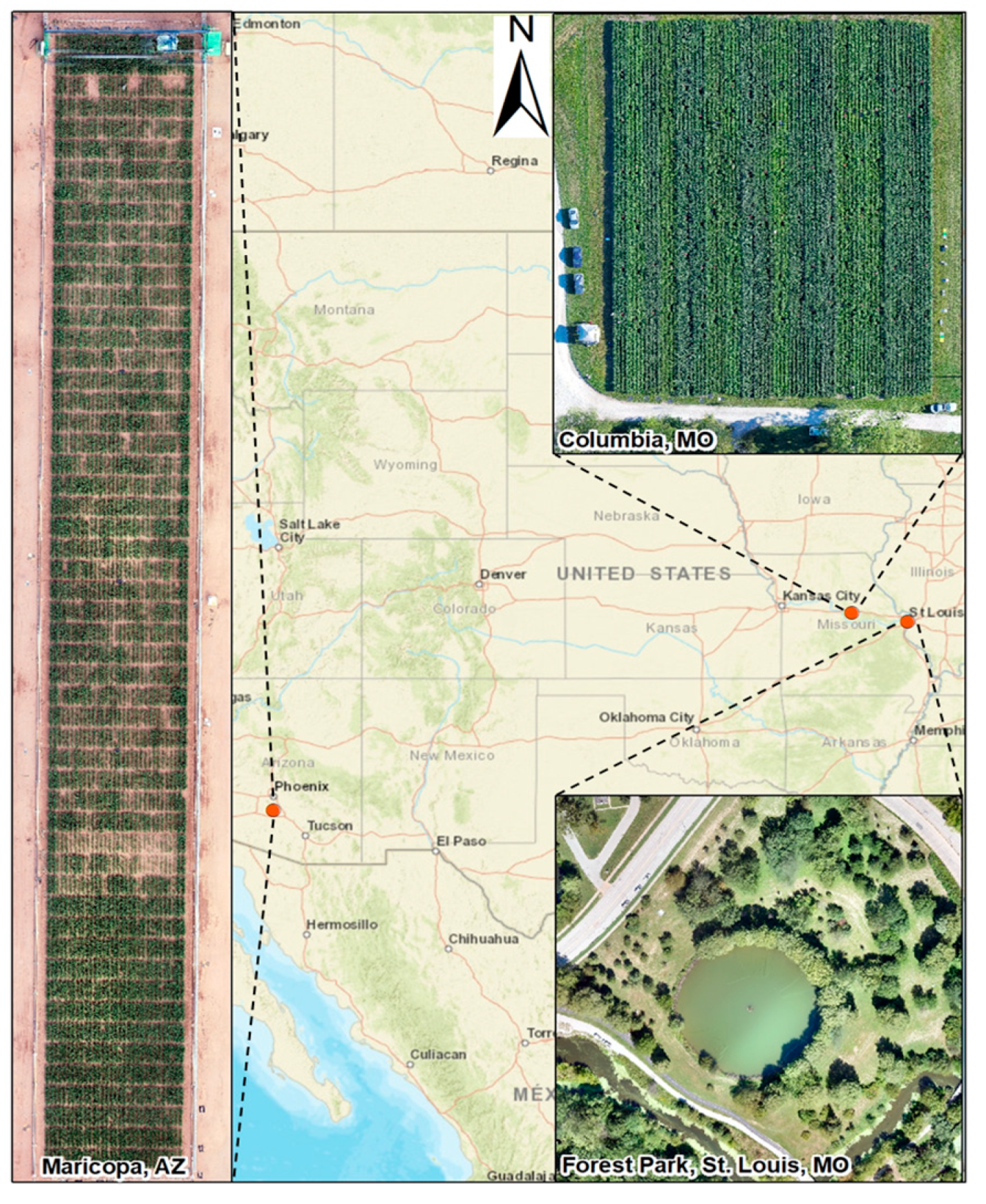
3. Test Sites and Case Studies

The experiments were conducted at three test sites representing different vegetation and climate conditions (Figure 2). The details of field setup, experimental design, and data collection for each case study are provided in the corresponding sections.

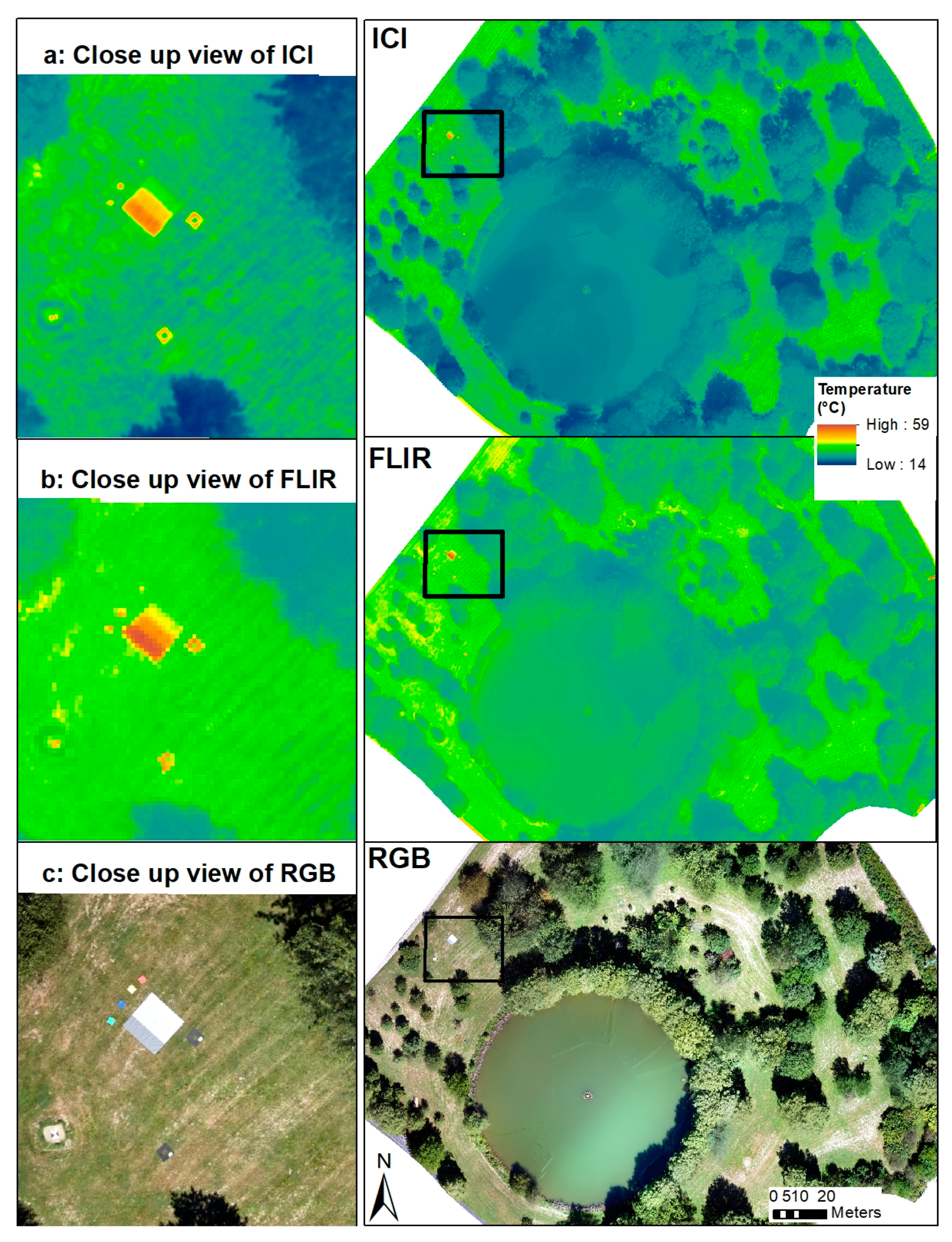
3.1. Case Study 1: Vegetation Monitoring in Forest Park, St. Louis, Missouri

In this case study, we focus on investigating the ICI and FLIR cameras with detailed analysis of thermal heat patterns that were observed over a heterogeneous terrain with land-cover and land-use, including buildup area, forest, grass, and water. Both of the cameras were mounted on DJI Matrice 600 Pro UAV (Figure 1a,b).

Field preparations were made prior to the UAV flights. A black and white reference panel was placed in the middle of the field, acting as an identifiable central point. Each corner of the field was marked with an unmovable point: a 1.8 m by 0.9 m grey tarp secured to the ground with stakes. Combined, these five points served as ground control points (GCPs). Flight paths were preprogrammed specifically for the study area using UgCS (SPH Engineering SIA, Latvia). UgCS is software that allows for precise flight planning for a variety of UAV systems.

The DJI Matrice 600 Pro UAVs (Figure 1a,b) were flown over a portion of Forest Park, in St. Louis, Missouri, USA on September 10th, 2018. The weather for the day was a high of 26.7 °C and a low of 15 °C, with mostly clear skies. The temperatures near the time of the ICI flight was 21.7 °C and 23.9 °C for the FLIR flight. The time difference between flights was approximately 1 h; the ICI flight started at 12:20 PM and the FLIR flight was at 11:23 AM. Due to the tall trees in the park, the UAV flights were conducted at 80 m height.

3.2. Case Study 2: Plant Phenotyping and Early Stress Detection near Columbia, Missouri

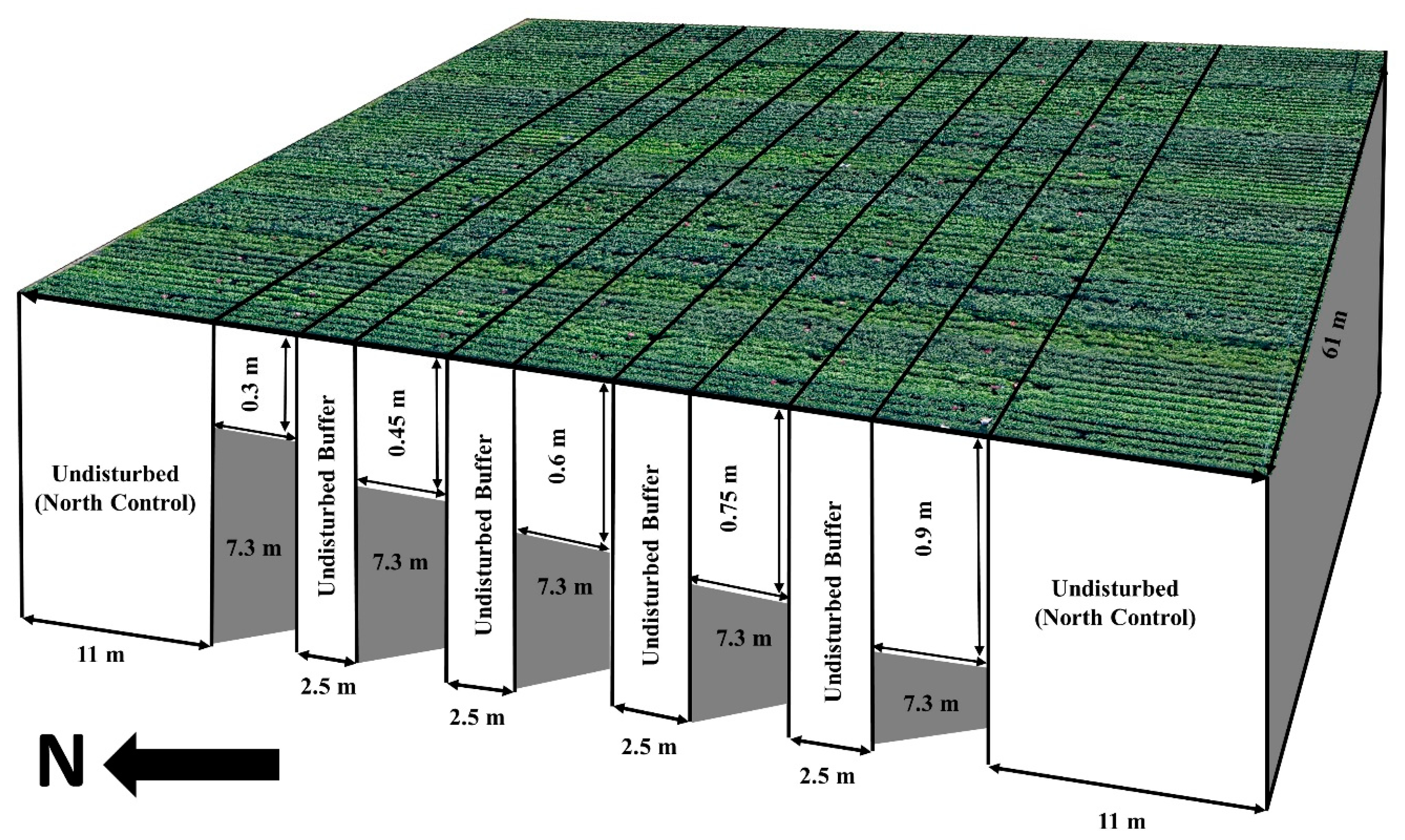
3.2.1. Experimental Setup

The experiment was conducted at the Bradford Research Center located near Columbia, Missouri, USA. The imaged field measures approximately 77 m in length and 65 m in width, and it has been modified to limit the maximum rooting depth of plants to different depths in different parts of the field, as described previously [42]. Briefly, approximately 6 m wide bands of soil were excavated perpendicular to the length of the field to either 0.3, 0.45, 0.6, 0.75, or 0.9 m depth, and a plastic barrier was installed to limit the rooting depth prior to refilling the excavated channels. On the north and the south ends, as well as between each of the rooting depth treatments, the soil profile was not disturbed, such that those areas represent normal field conditions at this site (Figure 3). Weed control was applied prior to soybean (Glycine max) planting on 18th April 2017. Soybean varieties ‘MO4301M’, ‘Dwight’, and ‘Pana’, and the two plant introductions, (PI) 398223 and 567201A, were planted in four row wide passes (0.76 m between rows) along the entire length (north-south orientation) of the field. Four replications, including one four-row pass of each entry, were planted with randomized entry location within replication. No insect or pest control was used. Unique plot identifiers were assigned for each entry x rooting depth treatment and replication. Temperatures on the day of data collection, 4th August 2017, were a high of 26 °C, a low of 14 °C, and an average of 20 °C. No significant rainfall occurred during that week.

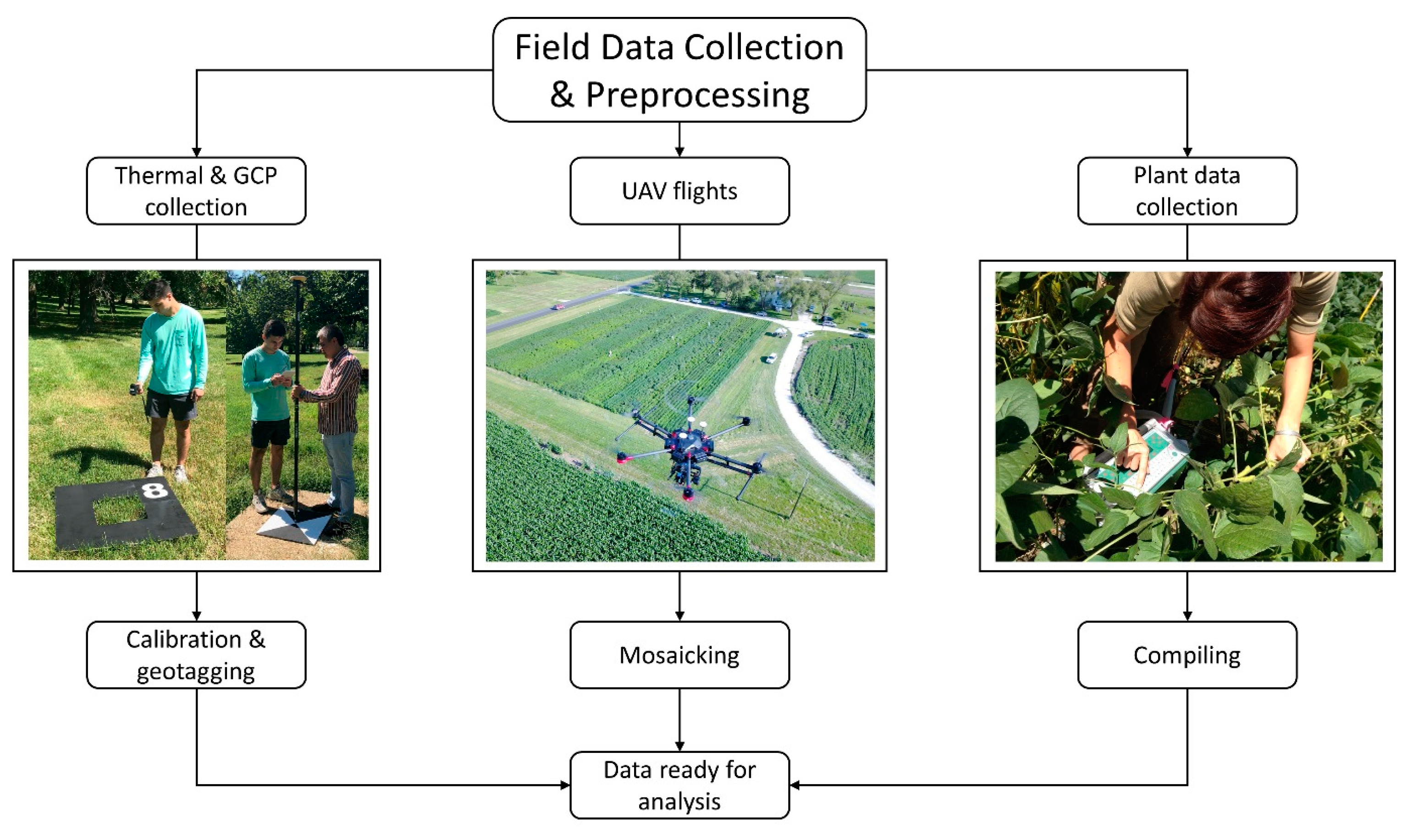
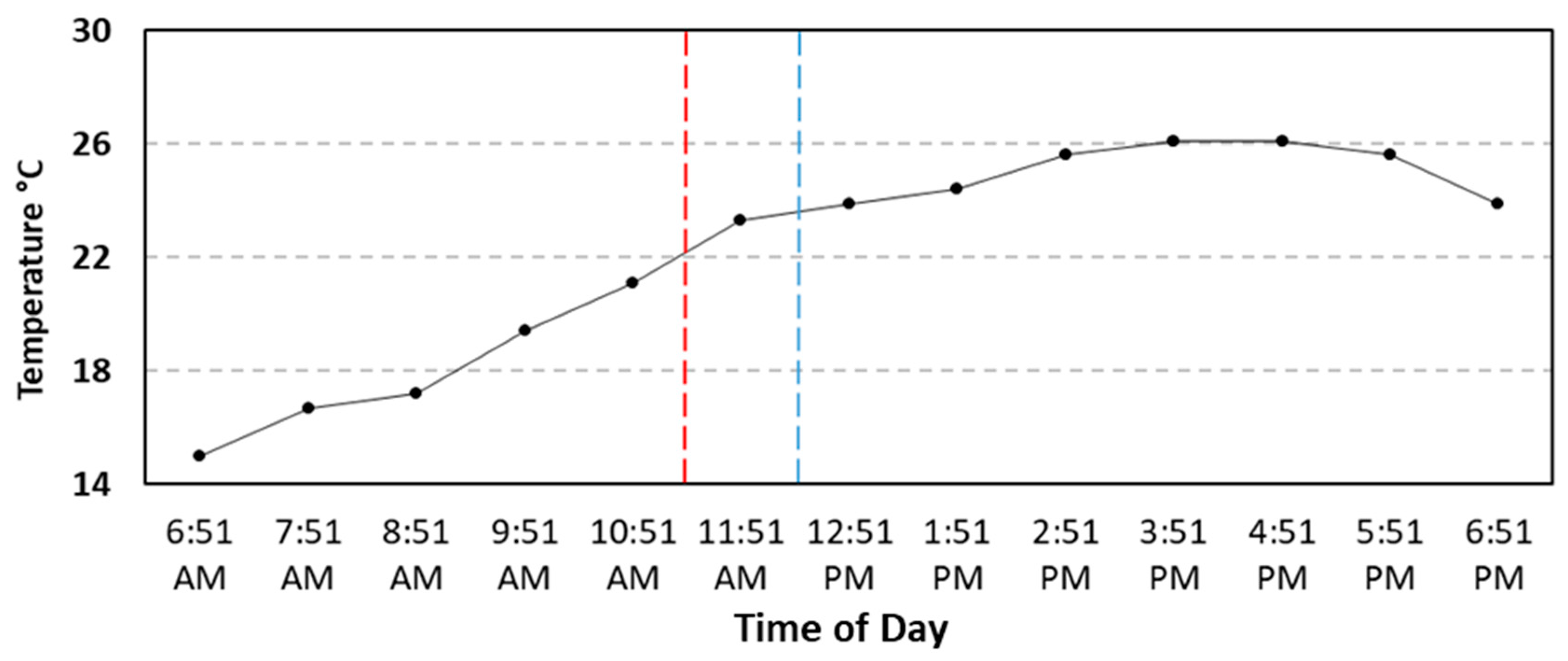
3.2.2. Data Collection

UAV images were collected using both ICI and FLIR cameras that were mounted onto custom- built DJI S1000+ platforms (Figure 1c,d). The ICI camera’s sensor lens was manually focused to the flight altitude (30 m). Camera capture settings were set at 1 s intervals. For the FLIR camera, a single image of the blackbody was taken in both the radiometric jpeg and 14-bit tiff formats. The camera was then set to also capture at 1 s intervals, but in a 14-bit tiff format. For both cameras, the gimbal was set to nadir. The ICI flight started at 11:50 AM and the FLIR flight at 12:30 PM on 4th August 2017. Both of the UAVs were flown at an altitude of 30 m with 80% side and front overlap. A DJI Mavic Pro (DJI, China) was flown soon after for RGB imagery acquisition from this field.

Ground based plant phenotypic traits were measured simultaneously during the UAV flights (Figure 4). For precise ground truthing of UAV data, the sampling locations within each plot were marked with wooden sticks for the duration of the experiment. Leaf Area Index (LAI) was measured using the LAI-2200C Plant Canopy Analyzer (LI-COR Inc., USA). This instrument allows for the user to operate under full sun conditions without any other requirements for sun angle. Measurements were conducted along a diagonal transect by placing the sensor on the ground between the row marked with the stakes and a neighboring row using the view restrictor to hide the user from the sensor Field of View (FOV). Two above canopy readings at the beginning and end of the rows were also made.

Plant height was measured for each plot, and the above ground plant biomass samples were collected by cutting the stems approximately 2 cm above the soil in the selected plots. After fresh weight determination, the plants were oven-dried at 60 °C until weights stabilized and dry samples were weighed to obtain above ground dry biomass.

Non-destructive measurements of leaf pigments were obtained on the uppermost, fully expanded trifoliate leaf at each sampling point using a DUALEX 4 Scientific (Force-A, France) handheld sensor from a plant within the marked sampling location. The leaf chlorophyll index (Chl), flavonol index (Flv), and Nitrogen Balance Index (NBI) are determined using the DUALEX 4 Scientific. The leaf chlorophyll index is calculated using (T₈₅₀ − T₇₁₀)/T₇₁₀, where T is leaf transmittance and the subscripts are wavelengths in nanometers (nm). The NBI is determined using [(Chl_AD + Chl_AB)/2]/(Flv_AD + Flv_AB), where the Flv is expressed as log(FRF_R/FRF_UV) using the far-red Chl fluorescence (FRF) emission excited by Red (R) or Ultra-Violate (UV) light. The subscripts AD and AB stand for adaxial and abaxial sides of the leaf, respectively. In this study, NBI was used as a measure of the plant nitrogen concentration.

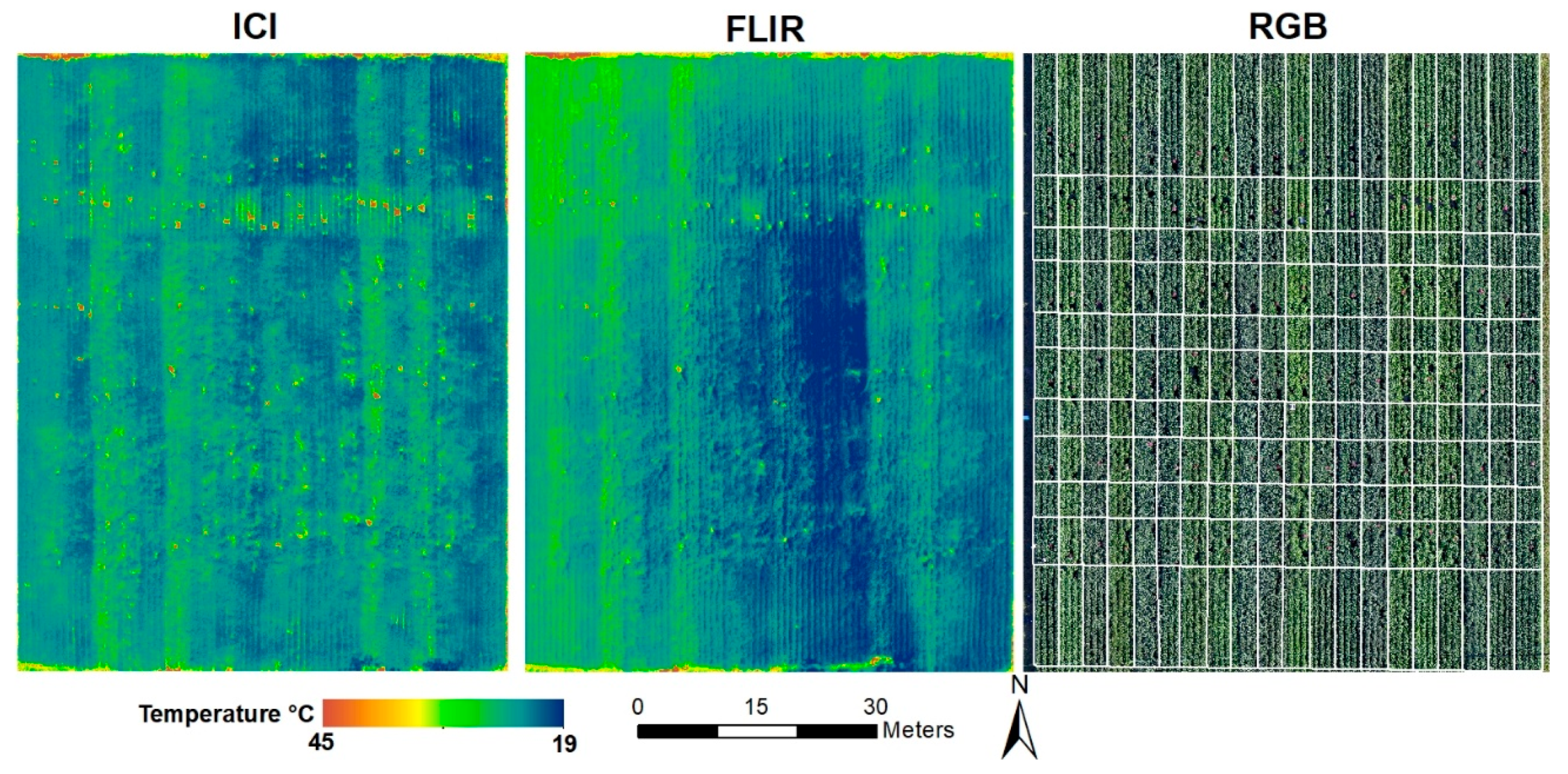
3.3. Case Study 3: High throughput Phenotyping at the Maricopa Agricultural Center

3.3.1. Experimental Setup

The third test site is the TERRA-REF field scanalyzer field at the Maricopa Agricultural Center, Maricopa, Arizona, USA. The dimensions of the field are 219 m long and 28 m wide. Details of the experimental site can be found in [43]. The site was planted with 168 recombinant inbred lines of Sorghum bicolor from the cross of parents SC56 and Tx7000. The experiment was arranged as a three replication row-column design. A custom plot grid was created to show the boundaries of each plot in the field, as shown in the RGB image of Figure 16 (Section 5.3.1). Metadata for the plots included unique identification numbers to distinguish between different genotypes and treatment areas. All plots on the edges were considered to be boundary plots and they were not factored when performing analytics. Thermal targets were placed on the outer perimeters of the field. Different from previous trials, plastic targets were used instead of the wooden variants.

3.3.2. Data Collection

UVA flights over the sorghum field were conducted on 11th October 2018. The temperature that day reached a high of 27.8 °C and a low of 16.7 °C, and averaged 22.2 °C. No rainfall was recorded. Relative humidity was approximately 57% during the flights. All three cameras (ICI, FLIR, and thermoMap) were used at this site. ICI and FLIR cameras were mounted on two DJI Matrice 600 Pro UAV systems (Figure 1a,b). The thermoMap camera was on the eBee (senseFly, USA) UAV system (Figure 1e,f). The thermoMap flight was performed at 10:45 AM, and subsequent flights by the FLIR and ICI sensors at were conducted at 11:30 AM and 11:45 AM, respectively. Images from a Sony RX10 (Sony Corporation, Japan; RGB imagery) and a RedEdge-M camera (MicaSense, Inc., Seattle, USA) were taken together with the ICI images, as all three cameras were mounted on the same platform (Figure 1a). The images from the Sony RX10 camera were used to classify and remove soil from the thermal images. All UAVs were flown at an altitude of 40 m. With the exception of the FLIR camera, all of the images were geotagged with proper spatial references during the flights.

During the UAV flight, ground thermal data was collected using the FLIR TG167 handheld thermal spot imager, with five readings per target. Ground based plant phenotypic traits, such as plant height, LAI, leaf nitrogen balance index (NBI), and Chlorophyll index (Chl), were measured from selected plots in each replication. The same instruments and procedures, as described for case study 2, were employed for plant traits measurement (see Section 3.2.1). Plant height, LAI, NBI, and Chl data were gathered over a period of three days, from 10th October to 12th October 2018.

4. Methods

4.1. UAV Image Pre-Processing

Mosaicking for the UAV thermal, RGB and multispectral images were performed using Pix4D (Pix4D S.A., Switzerland) software. Pix4D was specifically designed to process UAV data and it utilizes techniques that are rooted in both computer vision and photogrammetry to overcome the lack of precise sensor information, such as Global Position System (GPS) and Inertial Measurement Unit (IMU), information common in UAV data [44]. Different parameter adjustments, including changes to number of keypoints, image scale, and a targeted number of keypoints were used to produce optimal mosaics. Each mosaic was assessed for visual accuracy after processing.

Georeferencing and image registration was performed separately for each image using ground control point (GCP) coordinates that were collected using the Trimble Catalyst differential GPS system with <2 cm accuracy. The RGB imagery was georeferenced to GCPs of the field using ArcMap 10.4 (ESRI, USA). Thermal and multispectral images were then georeferenced using the aforementioned RGB image as a baseline.

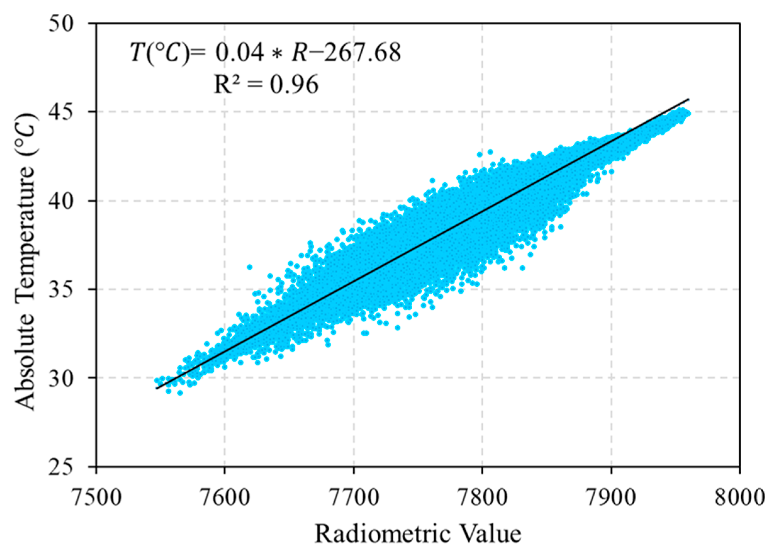
4.2. Thermal Image Calibration

At-sensor radiometric temperature that is captured by UAV integrated thermal cameras often needs to be converted to surface temperature in degrees Celsius (°C) or Fahrenheit (°F) by means of atmospheric and emissivity corrections for further applications. Radiometric distortions due to the atmospheric influence can be considered to be negligible in the case of low flight altitudes [45,46,47], e.g., at less than 30 m altitude above the ground level. A variety of approaches have been employed to convert at-sensor radiometric temperature to surface temperature in previous studies. Calibration equations/algorithms that were provided by the sensor vendor or processing software have been applied to achieve surface temperature information [48,49]. In addition, the empirical line method that is based on the linear relationship between at-sensor radiometric temperature and the corresponding surface temperature has been used in a variety of studies [47,50]. It is worth noting that radiometric calibration is sensitive to the environment, air temperature, humidity, and the temperature of other objects, which would have a substantial impact on the perceived temperature of the vegetation [51,52,53]. Moreover, uncooled microbolometer sensors also suffer from instability when the camera body temperature changes [47]. Accounting for the environmental conditions during UAV imagery acquisition in the thermal radiometric calibration procedure is very important for improved accuracy [51].

It is also essential to determine the optimal image-format in which to collect the data, and to develop an efficient workflow to pre-process the images into a format that is ready to be processed for orthomosaics. In this study, different strategies and procedures were employed for the radiometric calibration of ICI, FLIR, and thermoMap imagery, respectively.

Radiometric calibration for ICI thermal imagery was conducted using the IR-Flash tool that was provided by Infrared Cameras Inc. (https://infraredcameras.com/thermal-infrared-products/ir-flash-professional-thermal-imaging-software/). The IR-Flash tool provides batch processing for multiple images and then applies radiometric calibration using an internally installed factory calibration process. Additionally, the IR-Flash tool allows for the users to adjust environmental condition and imaging target related parameters, such as emissivity, transmission, and ambient temperature. We applied environment condition parameters that were obtained from nearby on-site weather stations. The radiometric JPG format images captured from the UAV integrated ICI camera were converted to 32 bit TIFF format with IR-Flash tool for further processing.

The FLIR camera provides radiometric JPEG and 14-bit TIFF imaging modes. The at-sensor radiometric values can be converted to temperature values in °C or °F using FLIR Tools that were provided by FLIR^® Systems, Inc. (https://www.flir.com/products/flir-tools/). FLIR Tools is an open-source software package that allows users to import, edit, visualize, and analyze images, and to conduct radiometric calibration. In addition, the FLIR Tools software provides options to adjust environmental conditions and imaging targets related parameters, such as emissivity, atmospheric temperature, relative humidity, and the distance between the camera and target. However, only the radiometric JPEG format imagery that has temperature data embedded in each pixel can be accessed by FLIR Tools and can be converted to radiometrically corrected temperature values in the TXT file format. Furthermore, FLIR Tools does not support converting multiple images in bulk; it only allows for the conversion of a single image at a time. Thus, in this study, the following procedures were employed to achieve radiometric calibration in bulk.

First, one image of the Model 1000 blackbody (Everest Interscience, Inc.) and the background scene was taken in radiometric JPEG. This was followed by taking one 14-bit tiff format image from the same scene immediately before the flight. The Model 1000 operates on a 9V Alkaline Transistor Battery. Its absolute measurement accuracy is 0.3 °C and thermal sensitivity is 0.1 °C (InfraredThermometry.com). Second, the radiometric JPEG image was loaded to FLIR Tools and relevant environmental parameters (air temperature, humidity, emissivity) were set using measurements from the respective weather stations. The converted and extracted temperature values were exported to TXT files [54,55]. The bias between the blackbody and image temperature was also determined. Lastly, each pixel value (radiometric value) in the 14-bit TIFF image was correlated to the corresponding value in the TXT file, which resulted in a linear model being used as a radiometric calibration equation (Figure 5, Equation (1)). It is worth noting that there is no single equation that can be used for images that are collected at different times and test sites, as environmental conditions vary significantly. Therefore, different equations were developed to account for changing environmental conditions at different study sites and times for every flight.

$$T\left(°\mathrm{C}\right)=0.04\times R-267.68$$

(1)

where $T\left(°\mathrm{C}\right)$ is the absolute temperature in degree Celsius and R is the radiometric value of FLIR thermal images.

The thermoMap camera captures radiometric TIFF imagery, and it has an integrated shutter for in-flight radiometric calibration (https://www.sensefly.com/camera/thermoMap/). It briefly closes its shutter at each waypoint, takes a photo of the back of the shutter, and automatically calibrates itself during the mission. To calibrate the level of grey in the photos, that photo is then compared to the temperature that was measured by the built-in temperature sensor [49,56,57]. In this case, the radiometric TIFF image was converted to temperature in degree Celsius directly with the equation designated for this camera with the Pix4DMapper software package [48,49]. The specific equation is as follows:

$$T\left(°\mathrm{C}\right)=0.01\times R-100$$

(2)

where T(°C) is the absolute temperature in Celsius degree and R is the radiometric value of thermoMap thermal images.

The ground measured temperatures from the various surfaces were compared with the corresponding temperatures in the radiometrically calibrated thermal imagery to evaluate the effectiveness of the calibration procedures along with temperature accuracy that was captured by different thermal cameras. Moreover, the thermal imagery was further corrected using the empirical line method based on ground temperature measurements [39,50].

4.3. Image Quality Assessment

The quality of the images was evaluated with respect to image naturalness and focal blur or motion blur using three no-reference based evaluation metrics, namely Vollath’s Correlation (VC) [58], Blur Metric (BM) [59], and Naturalness Image Quality Evaluator (NIQE) [60]. The VC, denoted as $F_4$ in Equation (3), is based on an autocorrelation function and it provides good performance in the presence of noise [61], and it is computed as

$$F_4={\displaystyle \sum }_{x=1}^{M-1}{\displaystyle \sum }_{y=1}^{N}f\left(x,y\right)f\left(x+1,y\right)-{\displaystyle \sum }_{x=1}^{M-2}{\displaystyle \sum }_{y=1}^{N}f\left(x,y\right)f\left(x+2,y\right)$$

(3)

In terms of image quality assessment, $f\left(x,y\right)$ represents the pixel value in the input image $f$ at the location $\left(x,y\right)$ with a dimension of $M\times N$.

The BM was derived from the blur discrimination of human perception by computing pixel intensity variations between the neighboring pixels. The general form of BM can be expressed as

$$BM=max\left({\mathit{\text{b\_F}}}_v, {\mathit{\text{b\_F}}}_h\right)$$

(4)

where ${\mathit{\text{b\_F}}}_v$ and ${\mathit{\text{b\_F}}}_h$ are the normalized sum of coefficients that were derived from vertical and horizontal directions, respectively. They can be calculated, as follows:

$${\mathit{\text{b\_F}}}_v=\frac{{{\displaystyle \sum }}_{x,y=1}^{M-1,N-1}{D}_{F_v\left(x,y\right)}-{{\displaystyle \sum }}_{x,y=1}^{M-1,N-1}{D}_{V_v\left(x,y\right)}}{{{\displaystyle \sum }}_{x,y=1}^{M-1,N-1}{D}_{F_v\left(x,y\right)}}$$

(5)

and

$${\mathit{\text{b\_F}}}_h=\frac{{{\displaystyle \sum }}_{x,y=1}^{M-1,N-1}{D}_{F_h\left(x,y\right)}-{{\displaystyle \sum }}_{x,y=1}^{M-1,N-1}{D}_{V_h\left(x,y\right)}}{{{\displaystyle \sum }}_{x,y=1}^{M-1,N-1}{D}_{F_h\left(x,y\right)}}$$

(6)

where $D_{F_v\left(x,y\right)}$, $D_{V_v\left(x,y\right)}$, $D_{F_h\left(x,y\right)}$, and $D_{V_h\left(x,y\right)}$ are the absolute difference images that were computed from the neighboring pixels in vertical and horizontal directions [59] using the original input image and blurred image with low-pass filters.

The NIQE is based on the construction of “quality aware” features derived from natural scene statistics (NSS) and fitting them to a multivariate Gaussian (MVG) model [60]. The final quality of the input image can be expressed as

$$D\left(v_1,v_2,{\Sigma }_1,{\Sigma }_2\right)=\sqrt{{\left(v_1-v_2\right)}^T{\left(\frac{{\Sigma }_1+{\Sigma }_2}{2}\right)}^{-1}\left(v_1-v_2\right)}$$

(7)

where $v_1$, $v_2$ and ${\Sigma }_1$, ${\Sigma }_2$, respectively, represent the mean vectors and covariance matrices of natural and the distorted MVG models.

Since the VC metric does not take into account focus measures from different scales in terms of the pixel neighborhood correlation, we propose a Multiscale VC (MVC) in this paper. The focal length of thermoMap is different than the other two cameras and it may lead to inaccurate image focus measures. The MVC is derived based on VC, however, it considers the correlation from multiple pixel distances, as expressed by

$$F_{MAC}=\frac{1}{K-1}{\displaystyle \sum }_{k=2}^K\left({\displaystyle \sum }_{x=1}^{M-1}{\displaystyle \sum }_{y=1}^{N}f\left(x,y\right)f\left(x+1,y\right)-{\displaystyle \sum }_{x=1}^{M-k}{\displaystyle \sum }_{y=1}^{N}f\left(x,y\right)f\left(x+k,y\right)\right)$$

(8)

where $k$ is a constant that represents the scale (i.e., pixel distance) during VC computation and $K$ is the maximum scale for computing MVC. In our experiments, we empirically set three scales for $k$, such that $K=4$.

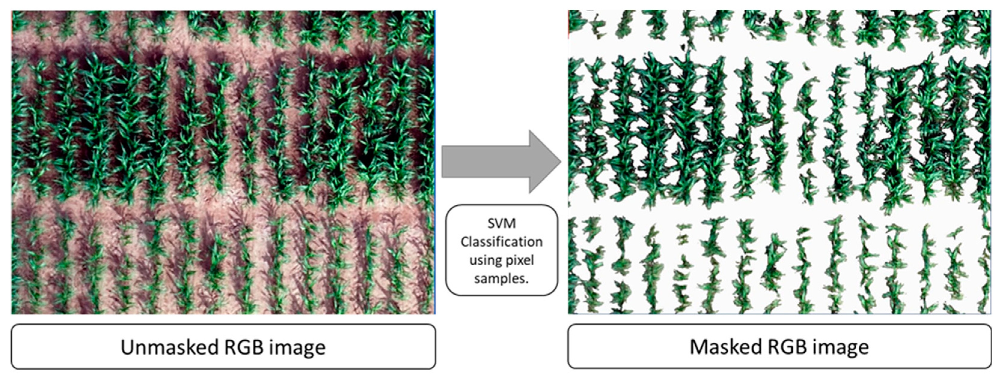
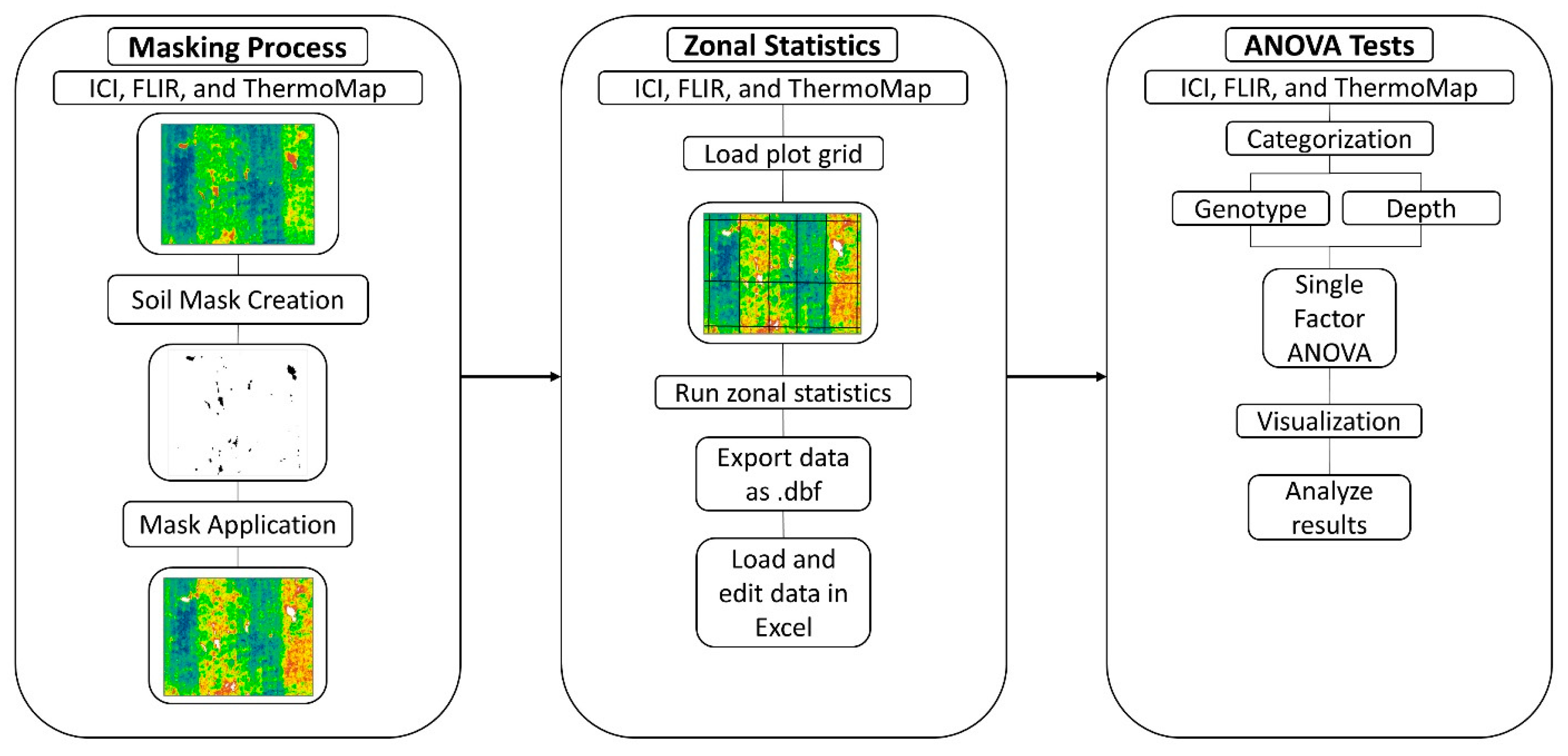
4.4. Processing of Images to Remove Non-Vegetation Pixels

For the most accurate canopy temperature data per plot, the thermal images required filtering of extraneous data. Areas that were outside of the study field itself were cropped. Due to the differences in flight heights and the pixel resolutions among the cameras the proportion of exposed soil varied among the test sites/flights. We used a machine learning based classification to eliminate soil (Figure 6). The vegetation was extracted from the RGB image by using a Support Vector Machine (SVM) based classifier following similar procedures to those that were outlined in [26]. The classification types were vegetation, exposed soil, shaded soil, and other (ground targets, metal objects, equipment). The classified results were then tested using approximately 50,000 training samples per class, with an overall accuracy of 97.3% and a Kappa coefficient of 0.97.

For case study 2 and 3, zonal statistics were performed per genotype using a grid shapefile created specifically for each plot representing a genotype. Metadata of the grid included row id and genotype name. The row id is a unique number that is given to a single rectangular plot. To run the zonal statistics process, the filtered thermal images and grid were selected as inputs, and they were run in separate instances. The outputs were tables containing the average temperature of each numbered plot. Border rows, acting as boundaries between different depth limits in case study 2, were excluded.

4.5. Statistical Analysis

4.5.1. ANOVA Test and Correlation Analysis

To quantitatively assess the results of the zonal statistics, one-way analysis of variance (ANOVA), followed by an honest significant difference (HSD) Tukey test (α = 0.05) was conducted to test the significant differences of crop genotypes and water treatment based on canopy temperature. In addition, Pearson’s correlation analysis were conducted between canopy temperature and plant traits. ANOVA tests and Pearson correlation analysis were performed using SPSS Statistics (IBM, USA). The plant traits used were biomass, LAI, grain yield, plant height, and stomatal conductance, depending on the test site and data availability for that test site. Each plant trait was used with the respective plot mean temperatures of thermal cameras for the analyses. For each parameter, however, plots where plant traits data was unavailable had to be excluded. The overall workflow of the statistical analysis process is shown in Figure 7.

To evaluate the accuracy of thermal imagery temperature against ground measured temperature, the coefficient of determination (R²), root mean square error (RMSE), and relative RMSE (RMSE%) were determined. These can be determined, as follows:

$$\mathrm{RMSE}=\sqrt{\frac{{{\displaystyle \sum }}_{i=1}^n{\left(y_i-{\widehat{y}}_i\right)}^2}{n-1}}$$

(9)

$$\mathrm{RMSE}\%=\frac{\mathrm{RMSE}}{\overline{y_i}}\times 100$$

(10)

where $y_i$ and ${\widehat{y}}_i$ are the measured and the predicted variables, respectively. $\overline{y_i}$ is the mean of measured value and $n$ is the total number of samples.

4.5.2. Heritability Analysis for Case Study 3

Heritability indicates the degree of variation in a phenotypic trait due to genetic variation within a specific population [62]. The heritability of a given trait at an individual environment is calculated as the ratio of genotypic variance to the total phenotypic variance [63]. A heritability value of 1.0 means that all of the variance in a population is caused by genetic differences among entries without any environmental or error effects. When heritability is zero, it is expected that all variation in the population is the result of environmental or error influences acting upon the individuals. We used the VHERITABILITY function available with GenStat from VSN International Ltd. (VSNi, UK), which calculates the generalized heritability for random terms in residual (or restricted) maximum likelihood (REML) analysis. The REML analysis utilizes linear models that can contain both fixed and random effects with several error terms that cannot be analyzed by ANOVA. The input table was a spreadsheet with plot numbers, genotypes, and the mean plot temperatures from the three flights. Coordinate for each plot was also included. The resulting value would then be applied with a function to determine the heritability percentage of the field with the different thermal cameras.

5. Results

5.1. Case Study 1: Vegetation Monitoring in Forest Park, St. Louis, Missouri

Figure 8 shows ICI, FLIR, and RGB imagery of the Forest Park study site. The findings from the comparison are the following:

The ICI imagery offered greater clarity in comparison to the FLIR. To maintain a comparative visual reading, the temperature range for both of the cameras was set to observed minimum and maximum temperature for both camera images, i.e., 14 °C to 59 °C. Overall, ICI imagery appeared to be visually smooth and sharp (see Figure 8 close-up views), which may be attributed to the fact that the ICI has a smaller NETD thermal sensitivity (0.02 °C) than the FLIR (0.05 °C). NETD thermal sensitivity, also called temperature resolution, measures how well a thermal imaging camera is able to distinguish between very small differences in thermal radiation. A lower NETD thermal sensitivity means that ICI should demonstrate better discrimination power and less noise, especially for low temperature areas (e.g., tree canopies and water) in the image in contrast to the image taken with the FLIR camera with higher NETD thermal sensitivity. In Figure 8a, the close-up target area is clearly defined in the ICI image, whereas the FLIR image is more pixilated, which is evident from Figure 8b, causing distortion of the targets in the data.

Regarding the temperature range over this test site, temperatures that were extracted from the FLIR images were higher overall with 17.46 °C to 58.48 °C, compared to 14.72 °C to 55.69 °C for those of the ICI imagery. The differences were in part due to the time differences between the two flights (Figure 9), and in part due to the FLIR camera’s reported temperature accuracy, which is +/− 5 °C. This contrasts with a much higher accuracy for the ICI (+/− 1 °C), offering more precise imagery.

In addition to visual assessment, the temperature accuracy captured by thermal cameras was evaluated as well. Figure 10 shows the comparison of the thermal camera temperature values over the ground thermal target location against the handheld thermal spot imager data taken on the ground. Using all eight temperature readings, an average was compiled for each target. This average value was then compared to the temperature value of the corresponding pixels within the thermal targets from the UAV images. Overall, the ICI produced a higher R² value (0.95) and 10% RMSE% as compared to the FLIR (R² = 0.92, RMSE% = 15%).

5.2. Case Study 2: Plant Phenotyping and Early Stress Detection near Columbia, Missouri

5.2.1. Visual Evaluation and Comparison

After mosaicking and calibration, both the ICI and FLIR images displayed acceptable data with both cameras allowing for visual differentiation of soybean genotypes. The ICI image exhibited slightly more detail, exhibiting more exposed soil than the FLIR image (Figure 11). This was corroborated by comparisons to the RGB image. Additionally, the ICI camera covers a wider spectral range, meaning that the differences in temperature were more visually enhanced as displayed in Figure 11. The FLIR image also displayed a variety of anomalies with the overall image that it provided. The northwestern corner, while mild when seen from the ICI camera, was considered “hot” by the FLIR camera. In addition to the corner, the center region of the field was unusually cool, which was displayed more consistently by the ICI camera. The study area did not undergo major changes between the flights, thus a sudden cooling within the field was considered to be unlikely.

Post flight calibration procedures for both thermal cameras were not identical, as each camera had its own specific process. ICI utilizes proprietary software, which converts the JPEG images to 32-bit TIFF files in an effective manner. The FLIR images required a separate calibration process using the FLIR Tools (FLIR Systems, USA) software.

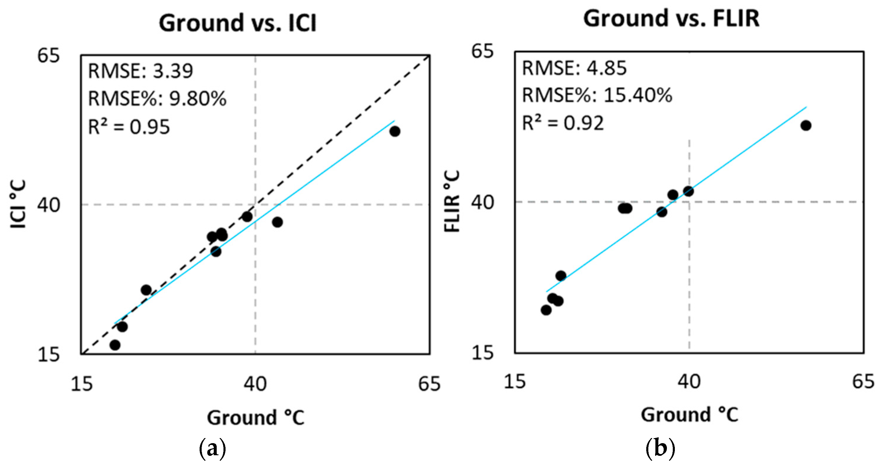
5.2.2. Temperature Accuracy Assessment

To validate the UAV derived temperatures from study site 2, a comparison was made with thermal data collected from ground thermal targets using the handheld thermal spot imager. Both thermal cameras showed high correlations, exhibiting R² values of 0.95 and 0.95, for the ICI and FLIR data sets, respectively (Figure 12). However, RMSE is 2.29 °C and 3.49 °C for the ICI and FLIR data, respectively, which is consistent with relative camera specifications that were claimed by manufacturers. It is worth noting that Figure 12 demonstrates the comparison between UAV-based thermal camera with ground-based thermal spot imager, each of which has its own accuracy and uncertainty. For example, the manufacturer claimed accuracy for each sensor are +/− 1 °C, +/− 5 °C, and +/− 1.5 °C for ICI, FLIR camera, and FLIR TG167 handheld thermal spot imager (ground truth), respectively. Each ground temperature measurement was compared to the corresponding pixel area that was seen in the UAV image. Minor differences between the ground and camera-derived temperatures were observed in absolute values, especially within lower temperature ranges. Both ICI and FLIR imagery resulted in an overestimation of temperatures at the higher temperature ranges, the deviation from the ground-based temperature measurements were greater for the FLIR (a better alignment along the 1:1 line for ICI than for FLIR).

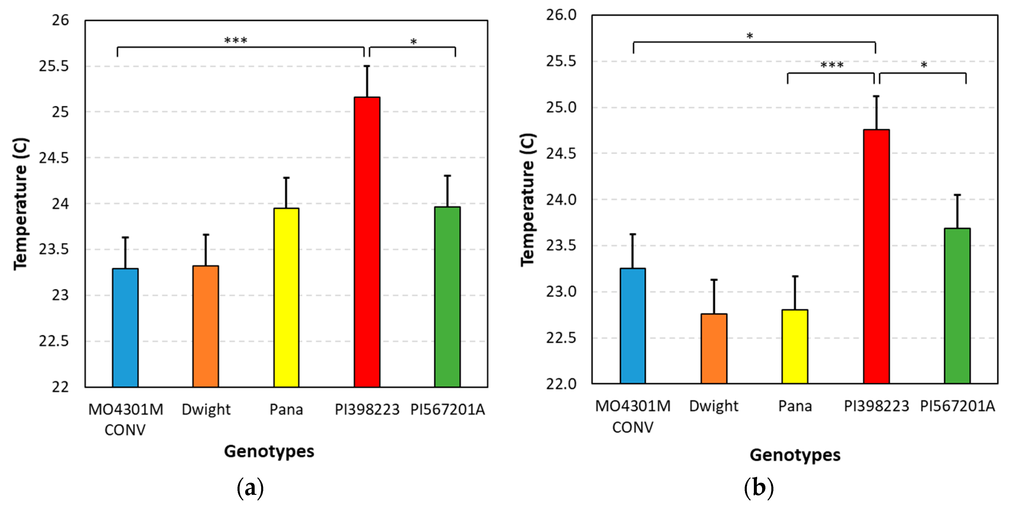
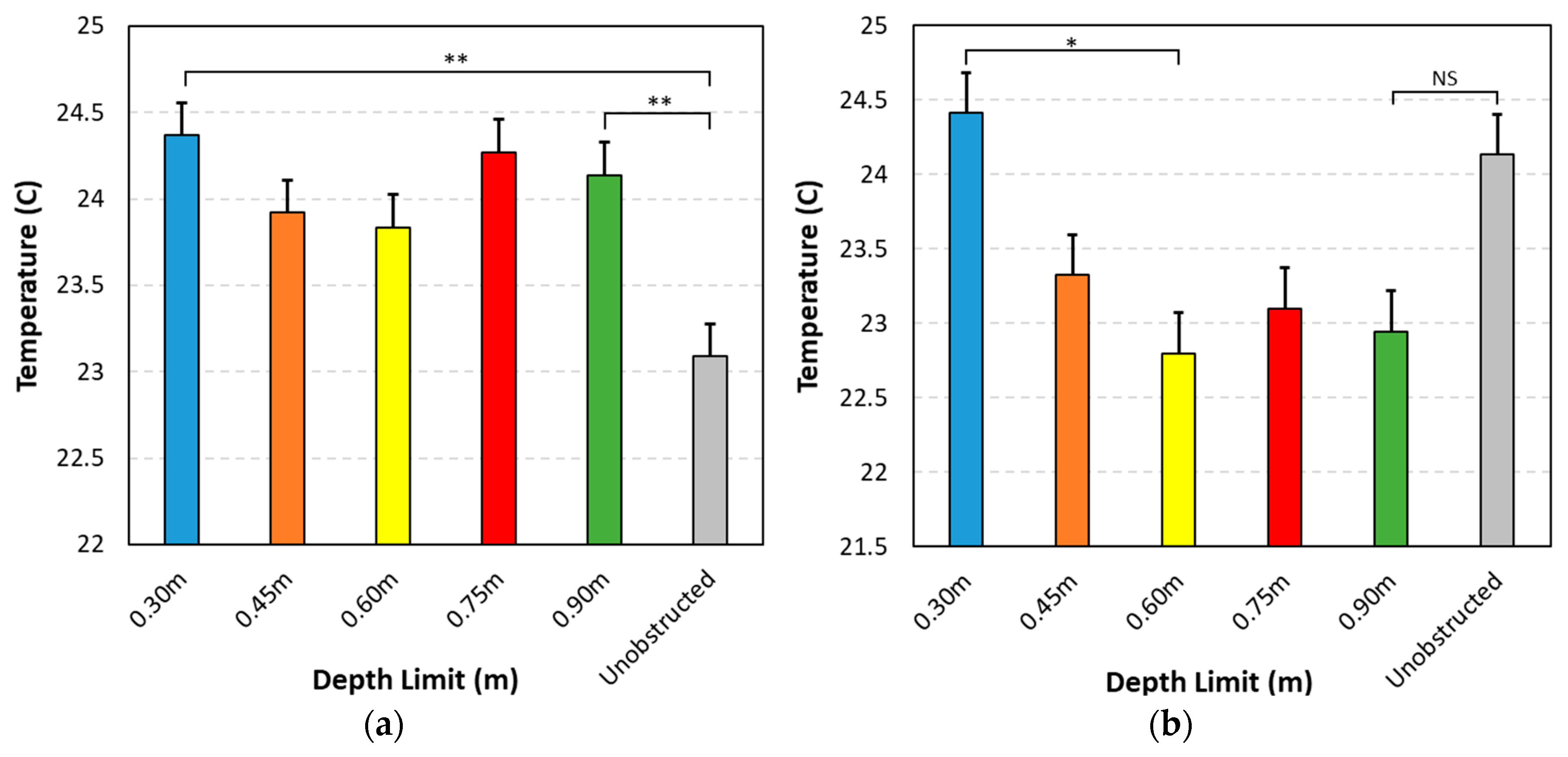
5.2.3. ANOVA Test for Different Soybean Genotypes and Rooting Depth Treatments

Figure 13 and Figure 14 show the overall single factor ANOVA results for both cameras, as categorized by genotype and rooting depth/water availability treatment. Statistical significance was also labeled, primarily for categories with notable statistical differences. Statistical significance was determined by performing additional ANOVA tests where specific category pairs were selected. Asterisks represent the statistical significance, primarily through the different p-values that were received from the paired ANOVA tests. A p-value of less than 0.05 is considered to be one asterisk, while a p-value less than 0.01 is considered to be two asterisks. A p-value smaller than 0.001 is considered to be three asterisks, which indicates the greatest statistical significance within the comparison. As shown by Figure 13 and Figure 14, both of the cameras can confidently differentiate the PI398223 and PI567201A genotypes. Statistical significance for PI398223 when compared to other genotypes yielded results above the 95% confidence interval. For the depth categorization, there were large discrepancies that were visible from the FLIR data. Despite the larger differences in temperatures, the p-value results for many FLIR pairs were larger than 0.05. Outputs that were above the 95% confidence threshold were only attainable for the ICI data when comparing the treated depths to the control. Comparisons that yielded a p-value greater than 0.05 were labeled Not Significant.

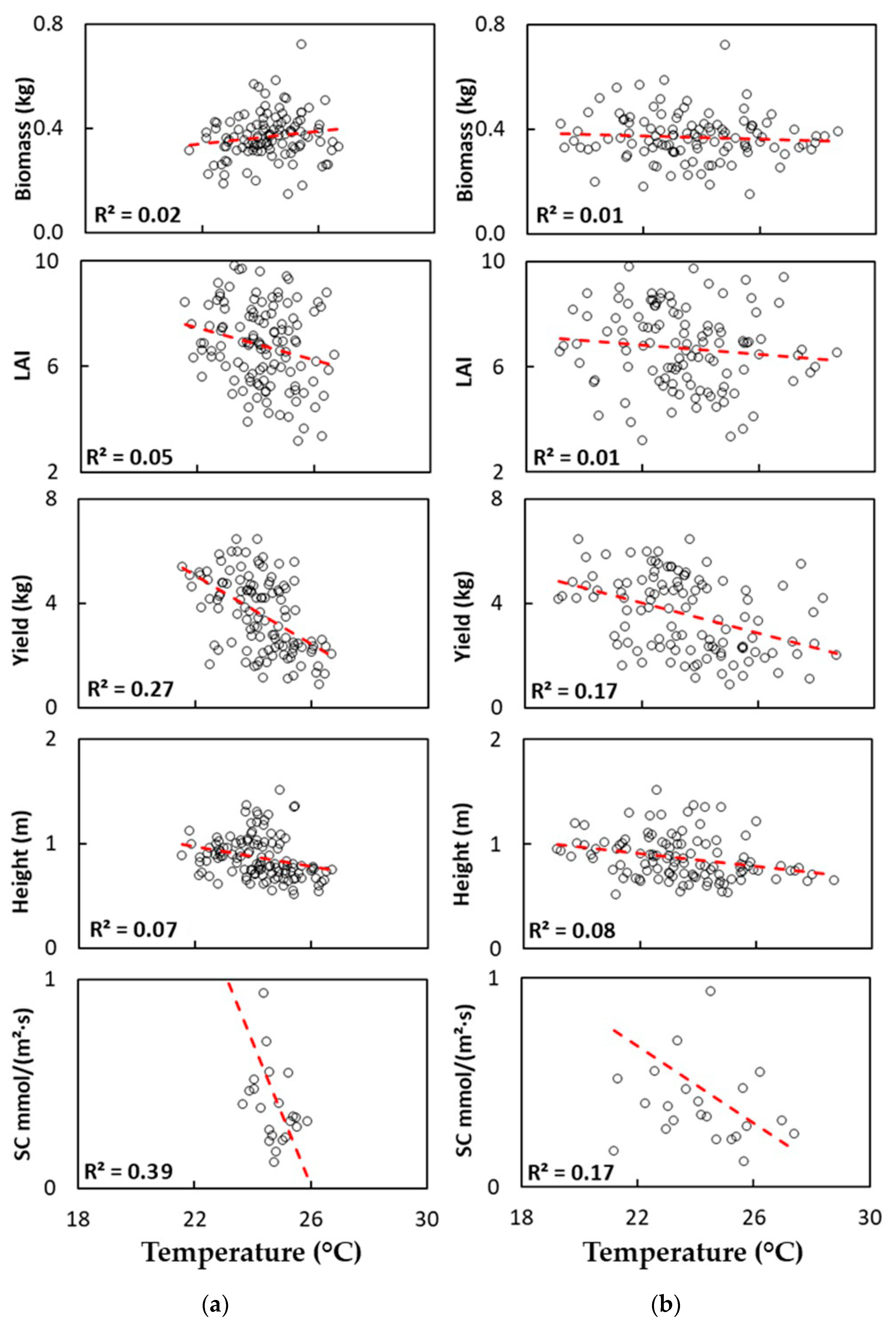
5.2.4. Correlation Analysis between Canopy Temperature and Plant Phenotypes

Table 2. Correlation coefficient between canopy temperature and soybean phenotypic traits.

Cameras	Biomass (g)	LAI	Grain Yield (g)	Height (cm)	SC (mmol/m2·s)
ICI (°C)	0.15	−0.23 *	−0.52 *	−0.26 **	−0.68 **
FLIR (°C)	−0.07	−0.03	−0.41 **	−0.28 **	−0.37 *

SC: Stomatal Conductance; *, **, *** represent significance levels of 0.05, 0.01, and 0.001 respectively.

and Figure 15 below show the results of the correlation analyses between canopy temperature and other phenotypes across all genotypes and rooting depth treatments. Canopy temperature and shoot biomass correlations were not significant (p > 0.05). Aside from biomass, the ICI data were significantly correlated with all other phenotypes. The FLIR data were correlated (p < 0.05) grain yield, plant height, and stomatal conductance. Both of the cameras achieved the 99% confidence threshold for plant height, despite having a lower correlation coefficient when compared to grain yield and stomatal conductance. The ICI data exhibited the strongest correlation and significance level with stomatal conductance, while the FLIR data performed similarly with yield.

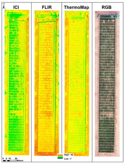
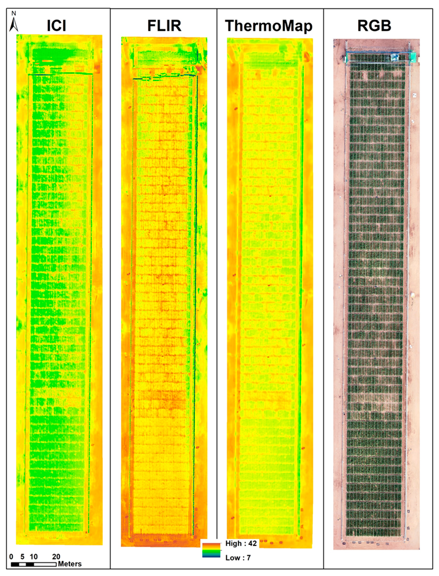
5.3. Case Study 3: High Throughput Phenotyping at Maricopa Agricultural Center

5.3.1. Visual Evaluation and Comparison

Figure 16 shows the qualitative comparison of the ICI, FLIR, and thermoMap cameras. The temperature ranges for each of the images varied due to the difference in capture time and as a result of the cameras being deployed on separate systems. One may expect that the FLIR and ICI camera should show higher temperatures than the thermoMap, since the FLIR and ICI flights were one hour later than the thermoMap. However, the ICI camera demonstrates a relatively cooler temperature gradient for the field, even though it was flown at approximately noon (thermoMap: 10:45 AM, FLIR: 11:30 AM, and ICI: 11:45 AM). This may be attributed to its smaller NETD thermal sensitivity and lower noise floor of ICI camera, which allows the detection of low temperature objects. Despite the temperature variations, all of the images could accurately discern between soil and plant canopy.

Unlike the test sites that were located in Missouri, the Maricopa, Arizona site represents an arid, semi-arid biome, and climate. During the time of data capture, more soil was exposed at the Maricopa site than at the other two sites. Given these considerations, a direct comparison of ground thermal measurements with UAV data was not conducted because surface temperature experienced significant change during the flights.

5.3.2. Heritability Analysis and Phenotype Estimation

After the soil pixels were removed using the machine learning based masks that were produced from the RGB imagery, zonal statistics were applied to gather average plot temperatures. The extracted data was then concatenated and loaded into Genstat, which is agriculture focused statistical analysis software from VSN International Ltd. (VSNi), UK. Extracted plot mean temperatures exhibited high heritability for ICI, FLIR, and thermoMap cameras, with values of 0.756, 0.744, and 0.729, respectively. Higher heritability indicates that a greater portion of plant trait variations is the result of genetic differences. All three cameras demonstrated that a significant portion of variability in plot temperatures (over 72%) was accounted for by genetic differences. Among the three cameras, ICI produced the highest heritability, which was followed by the FLIR and thermoMap.

Table 3. Pearson’s correlation coefficient between plot level mean temperatures and in-situ phenotypes.

Parameters	LAI		Height (cm)		NBI		Chl
Samples	193		237		165		165
Cameras	With soil	No soil	With soil	No soil	With soil	No soil	With soil	No soil
ICI	−0.266 **	−0.261 *	−0.597 **	−0.520 **	0.212 **	0.290 **	0.165 *	0.253 **
FLIR	−0.196 **	−0.142 *	−0.427 **	−0.263 **	−0.219 **	−0.359 **	−0.239 *	−0.373 **
thermoMap	−0.130	−0.132	−0.440 **	−0.465 **	−0.081	−0.060	−0.110	−0.078

** Correlation is significant at the 0.01 level (2-tailed). * Correlation is significant at the 0.05 level (2-tailed).

shows a Pearson’s correlation coefficient between plot level mean temperature values from the cameras and in-situ phenotypes, including LAI, canopy height, NBI, and Chl. Since LAI and canopy height are canopy structure information, a mixed pixel with soil component was used for analysis. NBI and Chl are leaf biochemical variables and soil was removed for NBI and Chl analysis. Thus, results were produced with and without soil information for comparative analysis. Overall, ICI temperature with soil was best correlated with LAI and canopy height at 0.01 significance. When soil effects were removed, the ICI temperature was still the strongest predictor of LAI and canopy height, with statistical significance at the 99% confidence interval. Following ICI, the FLIR results were superior to thermoMap for estimating LAI but they demonstrated the weakest correlation with canopy height among the three cameras. However, the relationship between leaf biochemical variables (NBI and Chl) and plot mean temperature was strongest with FLIR, which was followed by ICI. No statistically significant relationship was found between thermoMap temperature and LAI, NBI, and Chl, which was probably due to coarse ground sampling distance and larger NETD thermal sensitivity.

5.4. Image Quality Assessment and Comparison

Table 4. Quantitative assessment of image quality on 100 raw images for each test site. Note that the lower values of Naturalness Image Quality Evaluator (NIQE) and Blur Metric (BM), and higher values of Vollath’s Correlation (VC) and Multiscale VC (MVC) indicate a better image quality. The best score is highlighted in boldface.

Test Site	Cameras	Evaluation Metric
		NIQE	BM	VC	MVC
Forest Park, St. Louis, MO	ICI	3.312	0.340	201.451	400.034
	FLIR	4.031	0.355	163.206	337.699
Bradford, Columbia, MO	ICI	3.911	0.316	161.337	325.846
	FLIR	4.404	0.329	193.204	390.599
Maricopa, AZ	ICI	4.449	0.346	272.267	552.679
	FLIR	4.592	0.345	268.672	539.110
	thermoMap	5.678	0.3180	188.5250	382.812

VC: Vollath’s Correlation; BM: Blur Metric; NIQE: Naturalness Image Quality Evaluator; MVC: Multiscale VC.

shows a quantitative comparison of image quality of ICI, FLIR, and thermoMap captured images (i.e., 100 raw images for each camera) from three different test sites and

Table 5. Quantitative assessment of image quality on mosaicked images. Note that the lower values of NIQE and BM, and higher values of VC and MVC indicate a better image quality. The best score is highlighted in boldface.

Test Site	Cameras	Evaluation Metric
		NIQE	BM	VC	MVC
Forest Park, St. Louis, MO	ICI	3.059	0.359	838.689	1690.026
	FLIR	3.555	0.293	188.537	362.207
Bradford, Columbia, MO	ICI	4.100	0.330	688.574	1408.620
	FLIR	4.082	0.321	580.750	1,156.152
Maricopa, AZ	ICI	4.175	0.401	338.970	695.624
	FLIR	4.634	0.366	313.269	638.899
	thermoMap	8.481	0.489	102.327	242.439

VC: Vollath’s Correlation; BM: Blur Metric; NIQE: Naturalness Image Quality Evaluator; MVC: Multiscale VC.

shows image quality comparison using the mosaicked images generated from ICI, FLIR, and thermoMap cameras. The value of NIQE demonstrates the relationship between quantified image naturalness and perceptual image quality, while BM quantifies the image artifacts, including focal blur or motion blur [61]. Lower values of both NIQE and BM indicate better image quality than high values. In contrast, VC and MVC are image focus measures based on the autocorrelation. The higher the value of VC and MVC, the better the focus of the input images.

From Table 4 and Table 5, it can be seen that the performance of each camera is varied for each test site, although ICI and FLIR exhibited very competitive performance. More often than not, ICI provided better quality scores than FLIR (Table 4 and Table 5), which may be due to a joint contribution of its smaller f-stop and thermal sensitivity (Table 1). For raw images, ICI outperformed FLIR and thermoMap in almost all of the image quality metrics that were considered; however, FLIR showed overall smaller BM for mosaicked data, which was likely due to its better focus to infinity. Note that all images were normalized between 0 and 1 prior to the quality assessment, since the range of pixel intensity of these cameras varies.

6. Discussion

6.1. Thermal Cameras for Plant Phenotyping

The results of the current study demonstrated the value of thermal cameras mounted on UAVs to estimate a range of plant traits. Within the field of precision agriculture, the usage of UAV based thermal remote sensing has been proven to be beneficial for gathering data and providing useful analytics for plant related issues [38,64]. For genotype differentiation, the results of this study showed that thermal cameras could be used for this purpose, as demonstrated by Figure 13 and Figure 14. Due to differences in canopy architecture, leaf morphology, and physiology, different genotypes have individual properties that can contribute to differences in the emitted heat, which can be used to identify genotype differences. Among the five genotypes that were considered in the Columbia, MO test site, the ICI camera specifically identified greater genotype differences with the PI398223 soybean genotype, showing a higher average temperature as compared to the averages of others. Temperature variations among all of the genotypes were effectively explained by genotype difference and water treatment (Figure 14 and Figure 15), which is consistent with previous work [65] that utilized a similar method to differentiate between 92 different maize genotypes for screening drought adaptations.

Correlation analysis between plot average temperature and various plant traits demonstrated that there was no strong relationship or significance between temperatures and most of the plant traits that were considered, including LAI, biomass, and height for soybean growth at the Columbia, MO test site. However, the negative correlations between the extracted temperatures and yield were significant for both ICI and FLIR (Table 2), which is consistent with [40] and comparable to the results from [26,40]. Correlations of canopy temperature with canopy height and stomatal conductance were significant for both ICI and FLIR. The ICI exhibited the strongest correlation with stomatal conductance at 0.68 with a 99% confidence interval (Table 2).

6.2. Water Stress Detection

Plant water stress was identifiable from each image from the Columbia, MO study, which clearly showed the 0.3 m rooting depth treatment. As access to water is reduced, plants exhibit higher canopy temperature. For the ANOVA tests regarding the depth treatment factor, neither camera produced a conclusive image that was comparable to the genotype differentiation. A common factor was the 0.3 m row, but the other treatment rows had no similarities in relation to each other. An area of interest was the control row, which had no depth limit hindering root growth. The difference in average temperature for the control per image was greater than 1 °C. Hypothetically, the temperature of this region would be assumed as being constant or stable for both images, and, as each treatment gets deeper, the lower the temperature. The FLIR data showed that the control region was almost as hot as the 0.3 m region. In addition, the intermediate rows showed a much lower and probable range. From the ICI results of the ANOVA test, the middle rows exhibited the opposite of the FLIR, with all treatments being closer in temperature, with exception to the control area. The results were inconclusive regarding depth treatment differentiability. Neither camera in this case could accurately perform this function.

6.3. Impact of Camera Focal Length and Ground Sampling Distance

Spectral vegetation indices (VIs) are related to crop biochemical and biophysical traits, and they have been widely used to monitor crop growth and health [66,67,68,69]. In order to further investigate the impact of camera focal length and ground sampling distance on canopy temperature and crop phenotyping, Pearson’s correlation analysis between plot-level mean canopy temperature and several commonly used vegetation indices was applied for each camera at the Maricopa, AZ test site. Vegetation indices, including normalized difference vegetation index (NDVI), Green Normalized Difference Vegetation Index (GNDVI), and normalized difference red edge index (NDRE), respectively, were calculated using RedEdge-M camera (MicaSense, Inc., Seattle, USA). The correlation analysis was conducted under both with and without removing background soil.

Table 6. Correlation coefficient between plot mean temperature and vegetation indices.

VIs	NDVI		GNDVI		NDRE
Cameras	With soil	No soil	With soil	No soil	With soil	No soil
ICI	−0.857 **	−0.720 **	−0.846 **	−0.631 **	−0.803 **	−0.626 **
FLIR	−0.632 **	−0.371 **	−0.642 **	−0.341 **	−0.615 **	−0.302 **
thermoMap	−0.763 **	−0.749 **	−0.775 **	−0.631 **	−0.637 **	−0.468 **

** Correlation is significant at the 0.01 level (2-tailed).

shows the Pearson’s correlation coefficient (r) between canopy temperature and VIs with and without soil information. Canopy temperature from the ICI camera yielded the strongest correlation with all VIs in both with/without soil removal analyses, indicating that the ICI camera has greater potential in crop monitoring to some extent. The ICI camera is followed by the thermoMap camera in terms of canopy temperature and VIs correlation coefficient. The FLIR camera provided the weakest correlation among the cameras when compared to all VIs in both cases. However, it is worth mentioning that the FLIR camera presented slightly weaker but comparable performance with the thermoMap camera when soil was included in the analysis. In addition, the correlation coefficient between canopy temperature and VIs dropped significantly for the ICI and FLIR cameras when soil was removed, whereas it decreased only slightly for the thermoMap camera. This might be attributed to the relatively low ground sampling distance due to its 9 mm focal length and the larger thermal sensitivity of thermoMap. All of the flights were conducted at 40 m altitude, which produced approximately 5 cm ground sampling distance for both ICI and FLIR, and 10 cm for thermoMap imagery. This means that the thermoMap has a larger proportion of mixed pixels when compared to the ICI and FLIR with varying degree of soil information, which contributed to the greater variation in temperature values, even after soil removal. In other words, soil removal had little effect on the temperature-VI relationship for thermoMap. In contrast, the temperature-VI relationship was significantly changed after soil removal due to a greater proportion of removed soil signal as the result of the smaller ground sampling distance (spatial resolution) of the ICI and FLIR cameras. This was also evident from Table 3 that soil removal did not significantly affect the relationship between the thermoMap temperature and canopy structural (LAI, Height) and biochemical (NBI, Chl) variables. For both of the variables, change was significant for ICI and FLIR cameras due to the removal of soil information.

6.4. Limitations of the Study

To increase the diversity of experimental setup, we collected data at different altitudes. The Columbia, MO study site data was collected by UAV flights at an altitude of 30 m. In comparison, the Forest Park location was flown at approximately 80 m and the Maricopa site at 40 m. Although different topography required altitude changes, such as the tall trees that are present in Forest Park, a uniform flight height may provide consistency regarding data quality over different landscapes. When combined with the need to compare UAV imagery temperatures to ground measured temperatures, an inconsistent data collection method can hamper comparability of thermal image quality among different sites and ecosystems.

Thermal imaging cameras record longwave radiation or heat emitted from objects, which can be converted to a visible temperature map. The intensity of the radiation is determined by kinetic temperature of an object, emissivity, environmental (e.g., wind speed, humidity), and atmospheric (e.g., absorption from atmospheric water vapor, changes in upwelling and downwelling radiations) conditions. For UAV-based near surface thermal imaging, the effects of environmental conditions may have more considerable effects than atmospheric conditions that should be carefully treated and eliminated. Changes in sunlight conditions during multiple flights may alter kinetic temperature of the ground objects depending on climatic zones and the time length between the flights. In our study, due to the potential for an unwanted collision, the UAVs were not flown at the same times. The timing was evident for the Forest Park site, with a one-hour difference in flight time for the FLIR and ICI cameras. To minimize these effects for plant phenotyping, flights were scheduled to be continuous and there was an average of 15 min in between flight start times. Time differences can produce contrasting data with discrepancies in absolute temperature values. However, we found no significant effects of 15-min flight differences on the phenotype results and heritability analysis.

Correlating with the flight limitations were the differences between a copter and fixed-wing platforms. The flights in 2017 were conducted using two custom built DJI S1000+ octocopter platforms, which were integrated with an open source Pixhawk Autopilot. For the remainder of flights, the DJI Matrice 600 Pro UAV systems were used in conjunction with the ICI and FLIR cameras. The thermoMap camera was built within the eBee fixed-wing platform. A fixed-wing platform can offer similar performance and a longer flight time to gather more data, but it lacks the ability to hover and it requires a unique launch. Fixed-wing UAVs also lack the ability to carry relatively cumbersome gimbals that further enhance image stability as incorporated in the octo and hexacopter systems. With the combined differences of platforms, flight methods, and flight protocols, a more consistent approach in the future may prove superior.

Climate and geography, with regards to this study, was both a limitation and a benefit. For limitation, the Maricopa site was an outlier in terms of being an arid and hotter area in comparison to the more moderate and humid conditions of the Columbia and Forest Park sites. As displayed in Figure 16, the Maricopa site is located in a dry setting, lacking the grass and trees that are seen in the other sites. Despite the focus on the crop canopy, a dry surrounding can affect the thermal images that were collected by having a warmer air temperature and ground temperature, as the cameras utilize non-uniformity correction and flat field correction during the flights. This was evident by the lack of correlation with the UAV sensed target temperatures to the ground collected target temperatures. Combined with flight time differences and rising ground temperatures in a short time period, the comparison of data becomes more problematic, both with respect to comparisons among UAV-deployed cameras, as well as with ground truth data. Despite these limitations, the addition of a site with a vastly different climate was beneficial in illustrating the power of thermal cameras for plant phenotyping and vegetation monitoring.

Software and camera properties necessitated different calibration methods for the different systems. Furthermore, each camera has its’ own unique and proprietary onboard calibration system, including a non-uniformity correction (NUC), which may involve the use of methods, such as empirical line correction and other noise reduction techniques. This forces each dataset from the three cameras to be calibrated and the temperature to be converted differently. These differences may have contributed to the temperature variations, in addition to the flight time offsets due to flight logistics.

For a more advanced future project, using different crops for analysis could prove to be valuable for thermal based phenotyping. Only pure soybean and sorghum were analyzed for this study, with their respective genotypes. In a controlled setting, the thermal cameras have proven to be capable of discerning genotypes. In a more real-world application, a camera may be used to differentiate species of plants. By adding different crops, this can enhance the viability of utilizing thermal imagery for such purposes.

Last but not the least, it was not possible to draw an absolute conclusion in terms of image quality due to the fact that image quality can be distorted during acquisition, processing, compression, storage, and transmission procedures [70], as well as many other factors, such as weather condition, atmospheric effects, solar illumination, etc. Therefore, a more comprehensive evaluation would be required regarding image quality assessment to more directly evaluate sensors’ performance.

7. Conclusions

This study demonstrates that thermal cameras provide critical information for vegetation monitoring and plant phenotyping. Overall, all three thermal cameras considered (ICI 8640 P, FLIR Vue Pro R 640, and thermoMap) proved useful in vegetation monitoring and plant phenotyping. The main conclusions include:

• The ICI and FLIR cameras provided good image quality. The ICI camera provided the best score in terms of Naturalness Image Quality Evaluator (NIQE), while FLIR yielded better Blur Metric (BM) and Vollath’s Correlation (VC) scores. The ICI provided a more consistent and visually appealing result than the FLIR, but, as indicated by the quality tests, both of the cameras are capable of providing different sets of high-quality data.
• The ICI camera provided the best results for plant phenotyping, as its discerning ability was shown to be higher than those of the FLIR and thermoMap. Although respectable results were achieved by the FLIR, the ICI provided a more thorough and accurate result.
• Higher heritability indicates that a greater portion of plant trait variations is the result of genetic differences. The heritability of plot mean temperatures was highest when calculated based on the ICI camera, followed by FLIR and then thermoMap, with values of 0.756, 0.744, and 0.729, respectively. All three cameras demonstrated that over 72% of variability in plot mean temperatures was accounted for by genetic differences.
• The best overall thermal camera for precision agriculture and phenotyping based on this study was the ICI, as it performed well, with appealing spatial data, a close performance in image quality, with the highest value being exhibited for heritability. This is consistent with the relative camera specifications that were claimed by manufacturers.

References

1. Urban, J.; Ingwers, M.; McGuire, M.A.; Teskey, R.O. Stomatal conductance increases with rising temperature. Plant Signal. Behav. 2017, 12, e1356534. [Google Scholar] [CrossRef] [Green Version]
2. Urban, J.; Ingwers, M.W.; McGuire, M.A.; Teskey, R.O. Increase in leaf temperature opens stomata and decouples net photosynthesis from stomatal conductance in Pinus taeda and Populus deltoides x nigra. J. Exp. Bot. 2017, 68, 1757–1767. [Google Scholar] [CrossRef] [PubMed]
3. Sagan, V.; Maimaitiyiming, M.; Fishman, J. Effects of Ambient Ozone on Soybean Biophysical Variables and Mineral Nutrient Accumulation. Remote Sens. 2018, 10, 562. [Google Scholar] [CrossRef]
4. Seguin, B.; Lagouarde, J.P.; Savane, M. The Assessment of Regional Crop Water Conditions from Meteorological Satellite Thermal Infrared Data. Remote Sens. Environ. 1991, 35, 141–148. [Google Scholar] [CrossRef]
5. Bastiaanssen, W.G.M. SEBAL-based sensible and latent heat fluxes in the irrigated Gediz Basin, Turkey. J. Hydrol. 2000, 229, 87–100. [Google Scholar] [CrossRef]
6. Norman, J.M.; Anderson, M.C.; Kustas, W.P.; French, A.N.; Mecikalski, J.; Torn, R.; Diak, G.R.; Schmugge, T.J.; Tanner, B.C.W. Remote sensing of surface energy fluxes at 10(1)-m pixel resolutions. Water Resour. Res. 2003, 39, 1775. [Google Scholar] [CrossRef]
7. Xu, C.Y.; Qu, J.J.; Hao, X.J.; Cosh, M.H.; Prueger, J.H.; Zhu, Z.L.; Gutenberg, L. Downscaling of Surface Soil Moisture Retrieval by Combining MODIS/Landsat and In Situ Measurements. Remote Sens. 2018, 10, 210. [Google Scholar] [CrossRef]
8. Wang, J.; Ling, Z.W.; Wang, Y.; Zeng, H. Improving spatial representation of soil moisture by integration of microwave observations and the temperature-vegetation-drought index derived from MODIS products. ISPRS J. Photogramm. 2016, 113, 144–154. [Google Scholar] [CrossRef]
9. Leng, P.; Song, X.N.; Li, Z.L.; Wang, Y.W.; Wang, R.X. Toward the Estimation of Surface Soil Moisture Content Using Geostationary Satellite Data over Sparsely Vegetated Area. Remote Sens. 2015, 7, 4112–4138. [Google Scholar] [CrossRef] [Green Version]
10. Sepulcre-Canto, G.; Zarco-Tejada, P.J.; Sobrino, J.A.; Berni, J.A.J.; Jimenez-Munoz, J.C.; Gastellu-Etchegorry, J.P. Discriminating irrigated and rainfed olive orchards with thermal ASTER imagery and DART 3D simulation. Agric. For. Meteorol. 2009, 149, 962–975. [Google Scholar] [CrossRef]
11. Veysi, S.; Naseri, A.; Hamzeh, S.; Bartholomeus, H. A satellite based crop water stress index for irrigation scheduling in sugarcane fields. Agric. Water Manag. 2017, 189, 70–86. [Google Scholar] [CrossRef]
12. Leroux, L.; Baron, C.; Zoungrana, B.; Traore, S.B.; Lo Seen, D.; Begue, A. Crop Monitoring Using Vegetation and Thermal Indices for Yield Estimates: Case Study of a Rainfed Cereal in Semi-Arid West Africa. IEEE J. Sel. Top. Appl. Earth Obs. Remote Sens. 2016, 9, 347–362. [Google Scholar] [CrossRef]
13. Anderson, M.C.; Hain, C.; Wardlow, B.; Pimstein, A.; Mecikalski, J.R.; Kustas, W.P. Evaluation of Drought Indices Based on Thermal Remote Sensing of Evapotranspiration over the Continental United States. J. Clim. 2011, 24, 2025–2044. [Google Scholar] [CrossRef] [Green Version]
14. Anderson, M.C.; Allen, R.G.; Morse, A.; Kustas, W.P. Use of Landsat thermal imagery in monitoring evapotranspiration and managing water resources. Remote Sens. Environ. 2012, 122, 50–65. [Google Scholar] [CrossRef]
15. Kogan, F.N. Application of Vegetation Index and Brightness Temperature for Drought Detection. Adv. Space Res. 1995, 15, 91–100. [Google Scholar] [CrossRef]
16. Song, Y.; Fang, S.B.; Yang, Z.Q.; Shen, S.H. Drought indices based on MODIS data compared over a maize-growing season in Songliao Plain, China. J. Appl. Remote Sens. 2018, 12, 046003. [Google Scholar] [CrossRef]
17. Zaman-Allah, M.; Vergara, O.; Araus, J.; Tarekegne, A.; Magorokosho, C.; Zarco-Tejada, P.; Hornero, A.; Albà, A.H.; Das, B.; Craufurd, P. Unmanned aerial platform-based multi-spectral imaging for field phenotyping of maize. Plant Methods 2015, 11, 35. [Google Scholar] [CrossRef]
18. Wang, K.; Franklin, S.E.; Guo, X.; Cattet, M. Remote sensing of ecology, biodiversity and conservation: A review from the perspective of remote sensing specialists. Sensors 2010, 10, 9647–9667. [Google Scholar] [CrossRef]
19. Mulla, D.J. Twenty five years of remote sensing in precision agriculture: Key advances and remaining knowledge gaps. Biosyst. Eng. 2013, 114, 358–371. [Google Scholar] [CrossRef]
20. Walter, A.; Liebisch, F.; Hund, A. Plant phenotyping: From bean weighing to image analysis. Plant Methods 2015, 11, 14. [Google Scholar] [CrossRef]
21. Sadras, V.O.; Rebetzke, G.J.; Edmeades, G.O. The phenotype and the components of phenotypic variance of crop traits. Field Crop. Res. 2013, 154, 255–259. [Google Scholar] [CrossRef]
22. Lake, L.; Li, Y.L.; Casal, J.J.; Sadras, V.O. Negative association between chickpea response to competition and crop yield: Phenotypic and genetic analysis. Field Crop. Res. 2016, 196, 409–417. [Google Scholar] [CrossRef]
23. Madec, S.; Baret, F.; de Solan, B.; Thomas, S.; Dutartre, D.; Jezequel, S.; Hemmerle, M.; Colombeau, G.; Comar, A. High-Throughput Phenotyping of Plant Height: Comparing Unmanned Aerial Vehicles and Ground LiDAR Estimates. Front. Plant Sci. 2017, 8, 2002. [Google Scholar] [CrossRef] [PubMed]
24. Araus, J.L.; Kefauver, S.C.; Zaman-Allah, M.; Olsen, M.S.; Cairns, J.E. Translating High-Throughput Phenotyping into Genetic Gain. Trends Plant Sci. 2018, 23, 451–466. [Google Scholar] [CrossRef] [Green Version]
25. Yang, G.J.; Liu, J.G.; Zhao, C.J.; Li, Z.H.; Huang, Y.B.; Yu, H.Y.; Xu, B.; Yang, X.D.; Zhu, D.M.; Zhang, X.Y.; et al. Unmanned Aerial Vehicle Remote Sensing for Field-Based Crop Phenotyping: Current Status and Perspectives. Front. Plant Sci. 2017, 8, 1111. [Google Scholar] [CrossRef]
26. Maimaitijiang, M.; Ghulam, A.; Sidike, P.; Hartling, S.; Maimaitiyiming, M.; Peterson, K.; Shavers, E.; Fishman, J.; Peterson, J.; Kadam, S.; et al. Unmanned Aerial System (UAS)-based phenotyping of soybean using multi-sensor data fusion and extreme learning machine. ISPRS J. Photogramm. 2017, 134, 43–58. [Google Scholar] [CrossRef]
27. Jin, X.L.; Liu, S.Y.; Baret, F.; Hemerle, M.; Comar, A. Estimates of plant density of wheat crops at emergence from very low altitude UAV imagery. Remote Sens. Environ. 2017, 198, 105–114. [Google Scholar] [CrossRef]
28. Shi, Y.Y.; Thomasson, J.A.; Murray, S.C.; Pugh, N.A.; Rooney, W.L.; Shafian, S.; Rajan, N.; Rouze, G.; Morgan, C.L.S.; Neely, H.L.; et al. Unmanned Aerial Vehicles for High-Throughput Phenotyping and Agronomic Research. PLoS ONE 2016, 11, e0159781. [Google Scholar] [CrossRef]
29. Espinoza, C.Z.; Khot, L.R.; Sankaran, S.; Jacoby, P.W. High Resolution Multispectral and Thermal Remote Sensing-Based Water Stress Assessment in Subsurface Irrigated Grapevines. Remote Sens. 2017, 9, 961. [Google Scholar] [CrossRef]
30. Bellvert, J.; Zarco-Tejada, P.J.; Marsal, J.; Girona, J.; Gonzalez-Dugo, V.; Fereres, E. Vineyard irrigation scheduling based on airborne thermal imagery and water potential thresholds. Aust. J. Grape Wine R. 2016, 22, 307–315. [Google Scholar] [CrossRef]
31. Gonzalez-Dugo, V.; Goldhamer, D.; Zarco-Tejada, P.J.; Fereres, E. Improving the precision of irrigation in a pistachio farm using an unmanned airborne thermal system. Irrig. Sci. 2015, 33, 43–52. [Google Scholar] [CrossRef]
32. Park, S.; Ryu, D.; Fuentes, S.; Chung, H.; Hernyndez-Montes, E.; O’Connell, M. Adaptive Estimation of Crop Water Stress in Nectarine and Peach Orchards Using High-Resolution Imagery from an Unmanned Aerial Vehicle (UAV). Remote Sens. 2017, 9, 828. [Google Scholar] [CrossRef]
33. Di Gennaro, S.F.; Matese, A.; Gioli, B.; Toscano, P.; Zaldei, A.; Palliotti, A.; Genesio, L. Multisensor approach to assess vineyard thermal dynamics combining high resolution unmanned aerial vehicle (UAV) remote sensing and wireless sensor network (WSN) proximal sensing. Sci. Hortic. Amst. 2017, 221, 83–87. [Google Scholar] [CrossRef]
34. Berni, J.A.J.; Zarco-Tejada, P.J.; Sepulcre-Canto, G.; Fereres, E.; Villalobos, F. Mapping canopy conductance and CWSI in olive orchards using high resolution thermal remote sensing imagery. Remote Sens. Environ. 2009, 113, 2380–2388. [Google Scholar] [CrossRef]
35. Sullivan, D.G.; Fulton, J.P.; Shaw, J.N.; Bland, G. Evaluating the sensitivity of an unmanned thermal infrared aerial system to detect water stress in a cotton canopy. Trans. ASABE 2007, 50, 1955–1962. [Google Scholar] [CrossRef]
36. Han, M.; Zhang, H.H.; DeJonge, K.C.; Comas, L.H.; Trout, T.J. Estimating maize water stress by standard deviation of canopy temperature in thermal imagery. Agric. Water Manag. 2016, 177, 400–409. [Google Scholar] [CrossRef]
37. Hoffmann, H.; Jensen, R.; Thomsen, A.; Nieto, H.; Rasmussen, J.; Friborg, T. Crop water stress maps for an entire growing season from visible and thermal UAV imagery. Biogeosciences 2016, 13, 6545–6563. [Google Scholar] [CrossRef] [Green Version]
38. Ludovisi, R.; Tauro, F.; Salvati, R.; Khoury, S.; Mugnozza, G.S.; Harfouche, A. UAV-Based Thermal Imaging for High-Throughput Field Phenotyping of Black Poplar Response to Drought. Front. Plant Sci. 2017, 8, 1681. [Google Scholar] [CrossRef] [PubMed]
39. Gomez-Candon, D.; Virlet, N.; Labbe, S.; Jolivot, A.; Regnard, J.L. Field phenotyping of water stress at tree scale by UAV-sensed imagery: New insights for thermal acquisition and calibration. Precis Agric. 2016, 17, 786–800. [Google Scholar] [CrossRef]
40. Tattaris, M.; Reynolds, M.P.; Chapman, S.C. A Direct Comparison of Remote Sensing Approaches for High-Throughput Phenotyping in Plant Breeding. Front. Plant Sci. 2016, 7, 1131. [Google Scholar] [CrossRef]
41. Costa, J.M.; Grant, O.M.; Chaves, M.M. Thermography to explore plant-environment interactions. J. Exp. Bot. 2013, 64, 3937–3949. [Google Scholar] [CrossRef] [PubMed]
42. Hoyos-Villegas, V.; Houx, J.H.; Singh, S.K.; Fritschi, F.B. Ground-Based Digital Imaging as a Tool to Assess Soybean Growth and Yield. Crop Sci. 2014, 54, 1756–1768. [Google Scholar] [CrossRef]
43. Burnette, M.; Willis, C.; Kooper, R.; Maloney, J.D.; Ward, R.; Shakoor, N.; Newcomb, M.; Rohde, G.S.; Fahlgren, N.; Sagan, S.; et al. TERRA-REF Data Processing Infrastructure. In Proceedings of the Practice and Experience on Advanced Research Computing, Pittsburgh, PA, USA, 22–26 July 2018; p. 7. [Google Scholar]
44. Turner, D.; Lucieer, A.; Watson, C. An Automated Technique for Generating Georectified Mosaics from Ultra-High Resolution Unmanned Aerial Vehicle (UAV) Imagery, Based on Structure from Motion (SfM) Point Clouds. Remote Sens. 2012, 4, 1392–1410. [Google Scholar] [CrossRef] [Green Version]
45. Albertz, J. Einführung in die Fernerkundung: Grundlagen der Interpretation von Luft-und Satellitenbildern; Wiss. Buchges.: Darmstadt, Germany, 2001. [Google Scholar]
46. Gago, J.; Fernie, A.R.; Nikoloski, Z.; Tohge, T.; Martorell, S.; Escalona, J.M.; Ribas-Carbo, M.; Flexas, J.; Medrano, H. Integrative field scale phenotyping for investigating metabolic components of water stress within a vineyard. Plant Methods 2017, 13, 90. [Google Scholar] [CrossRef]
47. Berni, J.A.; Zarco-Tejada, P.J.; Suárez Barranco, M.D.; Fereres Castiel, E. Thermal and Narrow-Band Multispectral Remote Sensing for Vegetation Monitoring from an Unmanned Aerial Vehicle; Institute of Electrical and Electronics Engineers: Hoes Lane Piscataway, NJ, USA, 2009. [Google Scholar]
48. Agudo, P.; Pajas, J.; Pérez-Cabello, F.; Redón, J.; Lebrón, B. The Potential of Drones and Sensors to Enhance Detection of Archaeological Cropmarks: A Comparative Study Between Multi-Spectral and Thermal Imagery. Drones 2018, 2, 29. [Google Scholar] [CrossRef]
49. Raeva, P.L.; Šedina, J.; Dlesk, A. Monitoring of crop fields using multispectral and thermal imagery from UAV. Eur. J. Remote Sens. 2018, 1–10. [Google Scholar] [CrossRef]
50. Harvey, M.C.; Rowland, J.V.; Luketina, K.M. Drone with thermal infrared camera provides high resolution georeferenced imagery of the Waikite geothermal area, New Zealand. J. Volcanol. Geotherm. Res. 2016, 325, 61–69. [Google Scholar] [CrossRef]
51. Aubrecht, D.M.; Helliker, B.R.; Goulden, M.L.; Roberts, D.A.; Still, C.J.; Richardson, A.D. Continuous, long-term, high-frequency thermal imaging of vegetation: Uncertainties and recommended best practices. Agric. For. Meteorol. 2016, 228, 315–326. [Google Scholar] [CrossRef] [Green Version]
52. Torres-Rua, A. Vicarious calibration of sUAS microbolometer temperature imagery for estimation of radiometric land surface temperature. Sensors 2017, 17, 1499. [Google Scholar] [CrossRef]
53. Sugiura, R.; Noguchi, N.; Ishii, K. Correction of low-altitude thermal images applied to estimating soil water status. Biosyst. Eng. 2007, 96, 301–313. [Google Scholar] [CrossRef]
54. Zhang, Y.; Zhou, J.; Meng, L.; Li, M.; Ding, L.; Ma, J. A Method for Deriving Plant Temperature from UAV TIR Image. In Proceedings of the 2018 7th International Conference on Agro-geoinformatics (Agro-geoinformatics), Hangzhou, China, 6–9 August 2018; pp. 1–5. [Google Scholar]
55. Bergkamp, B.; Impa, S.; Asebedo, A.; Fritz, A.; Jagadish, S.K. Prominent winter wheat varieties response to post-flowering heat stress under controlled chambers and field based heat tents. Field Crop. Res. 2018, 222, 143–152. [Google Scholar] [CrossRef]
56. Kraaijenbrink, P.D.A.; Shea, J.M.; Litt, M.; Steiner, J.F.; Treichler, D.; Koch, I.; Immerzeel, W.W. Mapping Surface Temperatures on a Debris-Covered Glacier With an Unmanned Aerial Vehicle. Front. Earth Sci. 2018, 6, 64. [Google Scholar] [CrossRef]
57. Van der Sluijs, J.; Kokelj, S.V.; Fraser, R.H.; Tunnicliffe, J.; Lacelle, D. Permafrost Terrain Dynamics and Infrastructure Impacts Revealed by UAV Photogrammetry and Thermal Imaging. Remote Sens. 2018, 10, 1734. [Google Scholar] [CrossRef]
58. Vollath, D. Automatic focusing by correlative methods. J. Microsc. 1987, 147, 279–288. [Google Scholar] [CrossRef]
59. Crete, F.; Dolmiere, T.; Ladret, P.; Nicolas, M. The blur effect: Perception and estimation with a new no-reference perceptual blur metric. Proc. SPIE 2007, 64920I. [Google Scholar]
60. Mittal, A.; Soundararajan, R.; Bovik, A.C. Making a” Completely Blind” Image Quality Analyzer. IEEE Signal Process. Lett. 2013, 20, 209–212. [Google Scholar] [CrossRef]
61. Santos, A.; De Solorzano, C.O.; Vaquero, J.J.; Pena, J.M.; Malpica, N.; Del Pozo, F. Evaluation of autofocus functions in molecular cytogenetic analysis. J Microsc-Oxford 1997, 188, 264–272. [Google Scholar] [CrossRef] [Green Version]
62. Cullis, B.R.; Smith, A.B.; Coombes, N.E. On the design of early generation variety trials with correlated data. J. Agric. Biol. Environ. Stat. 2006, 11, 381–393. [Google Scholar] [CrossRef]
63. Makanza, R.; Zaman-Allah, M.; Cairns, J.E.; Magorokosho, C.; Tarekegne, A.; Olsen, M.; Prasanna, B.M. High-Throughput Phenotyping of Canopy Cover and Senescence in Maize Field Trials Using Aerial Digital Canopy Imaging. Remote Sens. 2018, 10, 330. [Google Scholar] [CrossRef]
64. Sheng, H.; Chao, H.; Coopmans, C.; Han, J.; McKee, M.; Chen, Y. Low-cost UAV-based thermal infrared remote sensing: Platform, calibration and applications. In Proceedings of the 2010 IEEE/ASME International Conference on Mechatronic and Embedded Systems and Applications, Qingdao, China, 15–17 July 2010; pp. 38–43. [Google Scholar]
65. Romano, G.; Zia, S.; Spreer, W.; Sanchez, C.; Cairns, J.; Araus, J.L.; Müller, J. Use of thermography for high throughput phenotyping of tropical maize adaptation in water stress. Comput. Electron. Agric. 2011, 79, 67–74. [Google Scholar] [CrossRef]
66. Asner, G.P. Biophysical and biochemical sources of variability in canopy reflectance. Remote Sens. Environ. 1998, 64, 234–253. [Google Scholar] [CrossRef]
67. Hansen, P.; Schjoerring, J. Reflectance measurement of canopy biomass and nitrogen status in wheat crops using normalized difference vegetation indices and partial least squares regression. Remote Sens. Environ. 2003, 86, 542–553. [Google Scholar] [CrossRef]
68. Aparicio, N.; Villegas, D.; Araus, J.; Casadesus, J.; Royo, C. Relationship between growth traits and spectral vegetation indices in durum wheat. Crop Sci. 2002, 42, 1547–1555. [Google Scholar] [CrossRef]
69. Babar, M.; Reynolds, M.; Van Ginkel, M.; Klatt, A.; Raun, W.; Stone, M. Spectral reflectance to estimate genetic variation for in-season biomass, leaf chlorophyll, and canopy temperature in wheat. Crop Sci. 2006, 46, 1046–1057. [Google Scholar] [CrossRef]
70. Wang, Z.; Bovik, A.C.; Sheikh, H.R.; Simoncelli, E.P. Image quality assessment: From error visibility to structural similarity. IEEE Trans. Image Process. 2004, 13, 600–612. [Google Scholar] [CrossRef]
Figure 1. Unmanned Aerial Systems (UAVs) and thermal cameras. Sony RGB and ICI cameras integrated on DJI M600 Pro hexa-copter (a), Headwall hyperspectral and FLIR cameras integrated on DJI M600 Pro hexa-copter (b), DJI S1000 octocopter and ICI camera (c), DJI S1000 octocopter and FLIR & camera array (d), and eBee UAV and thermoMap camera (e,f). Note: eBee UAV and thermoMap camera photos are obtained from this site: https://www.sensefly.com/.
Remotesensing 11 00330 g001
Figure 2. Test site locations and UAV-based RGB imagery from each site.
Remotesensing 11 00330 g002
Figure 3. Experimental field with modifications restricting plant roots to different depth and undisturbed areas on the northern and southern ends as well as between rooting depth treatments.
Remotesensing 11 00330 g003
Figure 4. The process for gathering thermal data, UAV imagery, and plant trait data. In the left photo, FLIR TG167 was used to take ground temperature readings over a thermal target, and Trimble Catalyst Differential GPS system was used to record accurate coordinates of ground control targets. In the middle, the UAV system was collecting data over the test site located in Bradford Research Extension Center, Columbia, Missouri. Right photo shows a LI-6400XT Portable Photosynthesis System being used to collect photosynthesis and stomatal conductance.
Remotesensing 11 00330 g004
Figure 5. Scatter plot of radiometric value from FLIR imagery and corresponding absolute temperature.
Remotesensing 11 00330 g005
Figure 6. Removal of non-vegetation pixels using Support Vector Machine (SVM) classification.
Remotesensing 11 00330 g006
Figure 7. Overall workflow of masking process, zonal statistics, and analysis of variance (ANOVA) tests.
Remotesensing 11 00330 g007
Figure 8. An overview of the Forest Park, St. Louis, USA location on the right the black boxes that indicate the target area which is zoomed into on the left. The items within the target area are two thermal targets, four different colored targets, a grey level tarp, and a ground control points (GCP).
Remotesensing 11 00330 g008
Figure 9. Air temperatures over the course of the day in Forest Park, St. Louis, Missouri, USA on 09/10/2018. The red and blue lines indicate to the approximate starting times of the flights with ICI (11:20 AM) and FLIR (12:20 PM) cameras.
Remotesensing 11 00330 g009
Figure 10. Comparison of ground-based temperatures of thermal targets obtained with a handheld temperature and temperatures of the ground targets based on ICI and FLIR imagery. (a) is the correlation between ICI camera and ground thermal target temperature values, and (b) shows the correlation between FLIR camera and ground thermal target temperature values.
Remotesensing 11 00330 g010
Figure 11. A comparative view of the Bradford test site in Columbia using different cameras. Solid lines on the RGB image to the right indicates plot boundary for different genotypes and rooting depth.
Remotesensing 11 00330 g011
Figure 12. A comparison of ground and UAV thermal data over the Bradford, Columbia test site. (a) is the correlation between ICI camera and ground thermal target temperature values, and (b) shows the correlation between FLIR camera and ground thermal target temperature values.
Remotesensing 11 00330 g012
Figure 13. ICI (a) and FLIR (b). The bars represent the average temperature of each genotype, with asterisks representing statistical significance tiers above. The number of asterisks represent p-value of 0.05 (one asterisk), 0.01 (two asterisks), and 0.001 (three asterisks).
Remotesensing 11 00330 g013
Figure 14. ICI (a) and FLIR (b). The bars represent the average temperature of each water treatment/depth, with statistical significance tiers above. The number of asterisks represents p-value of 0.05 (one asterisk), 0.01 (two asterisks), and 0.001 (three asterisks). NS refers to the results are not statistically significant. Note the large differences in temperature for the unobstructed region. In addition, the temperatures for other depths also had notable differences.
Remotesensing 11 00330 g014
Figure 15. Scatter plots of ICI (a) and FLIR (b) of temperature correlations to different plant phenotypes. The x-axis is the temperature in °C.
Remotesensing 11 00330 g015
Figure 16. An overview of the Maricopa study area captured by three different thermal cameras and a RGB camera for reference. thermoMap, FLIR, and ICI data were collected at 10:30 AM, 11:30 AM, and 11:45 AM local time on 11 October 2018.
Remotesensing 11 00330 g016